跳到论文正文
W Papers独立论文阅读器 arXiv:0801.2121 论文正文 计算阅读时间 · 0%
引用这篇论文根据当前论文元数据生成,正式投稿前建议核对。


License: arXiv.org perpetual non-exclusive license
arXiv:0801.2121v6 [nucl-th] 10 Nov 2008

On the time–modulation of the K–shell electron capture decay of H-like Pr58+140{{}^{140}}{\rm Pr}^{58+} ions produced by neutrino mass differences

A. N. Ivanov ††thanks: E-mail : ivanov@kph.tuwien.ac.at Affiliation: Atominstitut der Österreichischen Universitäten, Technische Universität Wien, Wiedner Hauptstraße 8-10, A-1040 Wien, Österreich, Affiliation: Stefan Meyer Institut für subatomare Physik, Österreichische Akademie der Wissenschaften, Boltzmanngasse 3, A-1090, Wien, Österreich    R. Reda Affiliation: Stefan Meyer Institut für subatomare Physik, Österreichische Akademie der Wissenschaften, Boltzmanngasse 3, A-1090, Wien, Österreich    P. Kienle ††thanks: E-mail : Paul.Kienle@ph.tum.de Affiliation: Stefan Meyer Institut für subatomare Physik, Österreichische Akademie der Wissenschaften, Boltzmanngasse 3, A-1090, Wien, Österreich Affiliation: Excellence Cluster Universe Technische Universität München, D-85748 Garching, Germany
August 24, 2026
Abstract

According to recent experimental data at GSI, the rate of the number of daughter ions Ce58+140{{}^{140}}{\rm Ce}^{58+}, produced by the nuclear K–shell electron capture (E​CEC) decay of the H–like ion Pr58+140{{}^{140}}{\rm Pr}^{58+}, is modulated in time with a period TE​C=7.06​(8)​secT_{EC}=7.06(8)\,{\rm sec} and an amplitude aE​C=0.18​(3)a_{EC}=0.18(3). We show that this phenomenon can be explained by neutrino mass differences and derive a value for the difference of squared masses Δ​m212=m22−m12=2.22​(3)×10−4​eV2\Delta m^{2}_{21}=m^{2}_{2}-m^{2}_{1}=2.22(3)\times 10^{-4}\,{\rm eV}^{2}.

PACS: 12.15.Ff, 13.15.+g, 23.40.Bw, 26.65.+t

Introduction

The experimental investigation of the K–shell electron capture (E​CEC) and β+\beta^{+} decays of the H–like Pr58+140{{}^{140}}{\rm Pr}^{58+} and the He–like Pr57+140{{}^{140}}{\rm Pr}^{57+} ions, has been recently carried out in the Experimental Storage Ring (ESR) at GSI in Darmstadt [1]. The obtained results showed a dependence of the weak decay rates on the electron structure of the heavy ions. As has been shown in [2], the experimental data on the ratios of the weak E​CEC and β+\beta^{+}–decay rates of the H–like Pr58+140{{}^{140}}{\rm Pr}^{58+} and the He–like Pr57+140{{}^{140}}{\rm Pr}^{57+} ions, obtained in GSI [1], can be described within standard theory of weak interactions of heavy ions and massless Dirac neutrinos [3] with an accuracy better than 3%3\,\%.

However, a very recent measurement of the time–dependence of the rate of the number of daughter ions Ce58+140{{}^{140}}{\rm Ce}^{58+} from the E​CEC–decay of the H–like Pr58+140{{}^{140}}{\rm Pr}^{58+} ion, i.e. Pr58+140→Ce58+140+νe{{}^{140}}{\rm Pr}^{58+}\to{{}^{140}}{\rm Ce}^{58+}+\nu_{e}, showed a time–modulation of the exponential decay with a period TE​C=7.06​(8)​sT_{EC}=7.06(8)\,{\rm s} and an amplitude aE​C=0.18​(3)a_{EC}=0.18(3) [4]11 1 For the E​CEC–decay of the H–like Pm60+142{{}^{142}}{\rm Pm}^{60+} ion the experimental value of the period of the time–modulation is TE​C=7.10​(22)​sT_{EC}=7.10(22)\,{\rm s} with the amplitude of the time–modulation aE​C=0.23​(4)a_{EC}=0.23(4) [4].. Since the rate of the number of daughter ions is defined by

d​NdE​C​(t)d​t=λE​C​(t)​Nm​(t),\displaystyle\frac{dN^{EC}_{d}(t)}{dt}=\lambda_{EC}(t)\,N_{m}(t), (1)

where λE​C​(t)\lambda_{EC}(t) is the E​CEC–decay rate and Nm​(t)N_{m}(t) is the number of mother ions Pr58+140{{}^{140}}{\rm Pr}^{58+}, the time–modulation of d​NdE​C​(t)/d​tdN^{EC}_{d}(t)/dt implies a periodic time–dependence of the E​CEC–decay rate λE​C​(t)\lambda_{EC}(t) [4]

λE​C​(t)=λE​C​{1+aE​C​cos⁡(2​π​tTE​C+ϕE​C)},\displaystyle\lambda_{EC}(t)=\lambda_{EC}\,\Big\{1+a_{EC}\cos\Big(\frac{2\pi t}{T_{EC}}+\phi_{EC}\Big)\Big\}, (2)

where aE​Ca_{EC}, TE​CT_{EC} and ϕE​C\phi_{EC} are the amplitude, period and phase of the time–dependent term [4].

Nowadays the existence of massive neutrinos, neutrino–flavour mixing and neutrino oscillations is well established experimentally and elaborated theoretically [5]. However, these phenomena concerned mainly the propagation of solar neutrinos and reactor anti–neutrinos in space and time combined with neutrino oscillations [5]. We show that the observed time–modulation of the rate of the number of daughter ions d​NdE​C​(t)/d​tdN^{EC}_{d}(t)/dt in the E​CEC–decay of the H–like Pr58+140{{}^{140}}{\rm Pr}^{58+} ions is not caused by neutrino oscillations but can be explained by a kind of quantum beats [6] due to mass differences of neutrino mass–eigenstates [5]. This can provide a new method for studying of massive neutrino mixing, neutrino mass differences and neutrino vacuum polarisation.

Amplitudes of E​CEC–decays of H–like heavy ions

The Hamilton operator HW​(t){\rm H}_{W}(t) of the weak interactions, responsible for the E​CEC and β+\beta^{+} decays of the H–like heavy ions, can be taken in the standard form [3] but accounting for the neutrino–flavour mixing [5] (see also [7]–[9]). This gives HW​(t)=∑jUe​j​HW(j)​(t){\rm H}_{W}(t)=\sum_{j}U_{ej}{\rm H}^{(j)}_{W}(t), where Ue​jU_{ej} are matrix elements of the neutrino mixing matrix UU [5]. The Hamilton operator of the weak interactions HW(j)​(t){\rm H}^{(j)}_{W}(t) is defined by

HW(j)​(t)=GF2​Vu​d​∫d3​x​[ψ¯n​(x)​γμ​(1−gA​γ5)​ψp​(x)]\displaystyle{\rm H}^{(j)}_{W}(t)=\frac{G_{F}}{\sqrt{2}}V_{ud}\!\!\int\!\!d^{3}x[\bar{\psi}_{n}(x)\gamma^{\mu}(1-g_{A}\gamma^{5})\psi_{p}(x)]
×[ψ¯νj​(x)​γμ​(1−γ5)​ψe−​(x)],\displaystyle\times[\bar{\psi}_{\nu_{j}}(x)\gamma_{\mu}(1-\gamma^{5})\psi_{e^{-}}(x)], (3)

with standard notations [2, 3].

The massive neutrinos νj\nu_{j} in the final state of the E​CEC–decay m→d+νem\to d+\nu_{e}, where mm and dd are the mother and daughter ions, are indistinguishable in principle, since the electron is entangled with the electron neutrino νe\nu_{e} only [8], which is the superposition of the neutrino mass–eigenstates |νe⟩=∑jUe​j∗​|νj⟩|\nu_{e}\rangle=\sum_{j}U^{*}_{ej}|\nu_{j}\rangle [5]. Such an indistinguishability of massive neutrinos νj\nu_{j} requires to take the amplitude A​(m→d+νe)​(t)A(m\to d+\nu_{e})(t) of the E​CEC–decay as a coherent sum of the amplitudes A​(m→d+νj)​(t)A(m\to d+\nu_{j})(t) of the m→d+νjm\to d+\nu_{j} decays, describing three alternative ways of the evolution of the initial system, i.e. the mother ion mm into the daughter ion dd. According to Feynman [10], the probability amplitude of the evolution of the quantum system should be taken in the form of a coherent sum of the probability amplitudes of every alternative way of the evolution (see also [11]) in contrast to the recent assertion by Giunti [12] and Kienert et al. [13]. As a result we get

A⁡(m→d+νe)​(t)=∑jUe​j​A​(m→d+νj)​(t),\displaystyle A(m\to d+\nu_{e})(t)=\sum_{j}U_{ej}A(m\to d+\nu_{j})(t), (4)

where the coefficients Ue​jU_{ej} take into account that the electron couples to the electron neutrino only.

In the standard time–dependent perturbation theory [14] the amplitudes A​(m→d+νj)​(t)A(m\to d+\nu_{j})(t), defined in the rest frame of the mother ion, are given by

A⁡(m→d+νj)​(t)=\displaystyle A(m\to d+\nu_{j})(t)=
=−i∫−∞tdτeε​τ⟨d(q→)νj(k→j)|HW(j)(τ)|m(0→)⟩,\displaystyle=-i\int^{t}_{-\infty}d\tau\,e^{\textstyle\,\varepsilon\,\tau}\,\langle d(\vec{q}\,)\nu_{j}(\vec{k}_{j})|H^{(j)}_{W}(\tau)|m(\vec{0}\,)\rangle, (5)

where q→\vec{q} and k→j\vec{k}_{j} are 3–momenta of the daughter ion and the neutrino mass–eigenstate νj\nu_{j}, respectively. For the regularization of the integral over time we use the ε→0\varepsilon\to 0 regularization procedure.

For the description of the time modulated interference term in the E​CEC–decay rate of the H–like heavy ion Eq.(2) we assume a non–conservation of 3–momenta of neutrino mass–eigenstates in order to deal with differences of 3–momenta of massive neutrinos playing important role in our analysis of the interference term. Non–conservation of 3–momenta of massive neutrinos can be caused by the uncertainties of momenta of the bound electron, proton and neutron in the elementary e−+p→n+νje^{-}+p\to n+\nu_{j} transition of the E​CEC–decay of the H–like heavy ion (see also [15]).

A quantum mechanical description of the E​CEC–decays of the H–like heavy ions with different 3–momenta of neutrino mass–eigenstates can be carried out using the wave functions of massive neutrinos in the form of the Gaussian wave packets [16]

ψνj​(r→,t)=(2​π​δ2)3/2​∫d3​k(2​π)3​e−12​δ2​(k→−k→j)2\displaystyle\psi_{\nu_{j}}(\vec{r},t)=(2\pi\delta^{2})^{3/2}\int\frac{d^{3}k}{(2\pi)^{3}}\,e^{\,-\,\frac{1}{2}\,\delta^{2}(\vec{k}-\vec{k}_{j})^{2}}
×ei​k→⋅r→−i​Ej​(k→)​t​uνj​(k→,σνj),\displaystyle\times\,e^{\textstyle\,i\vec{k}\cdot\vec{r}-iE_{j}(\vec{k}\,)t}u_{\nu_{j}}(\vec{k},\sigma_{\nu_{j}}), (6)

where δ\delta is a spatial spread of the massive neutrino νj\nu_{j}, k→j\vec{k}_{j} is the neutrino momentum and Ej​(k→)=k→ 2+mj2E_{j}(\vec{k}\,)=\sqrt{\vec{k}^{\,2}+m^{2}_{j}} is the energy of a plane wave with the momentum k→\vec{k}, uνj​(k→,σνj)u_{\nu_{j}}(\vec{k},\sigma_{\nu_{j}}) is the Dirac bispinor of the massive neutrino νj\nu_{j}. In the limit δ→∞\delta\to\infty the wave function (6) reduces to a plane wave.

Following [2], we obtain the amplitude of the E​CEC–decay as a function of time tt

A⁡(m→d+νe)​(t)=−3​2​Mm​2​Ed​(q→)\displaystyle A(m\to d+\nu_{e})(t)=-\sqrt{3}\sqrt{2M_{m}2E_{d}(\vec{q}\,)}
×ℳGT​⟨ψ1​s(Z)⟩​(2​π​δ2)3/2​∑jUe​j​Ej​(q→)\displaystyle\times\,{\cal M}_{\rm GT}\,\langle\psi^{(Z)}_{1s}\rangle(2\pi\delta^{2})^{3/2}\sum_{j}U_{ej}\sqrt{E_{j}(\vec{q}\,)}
×e−12​δ2​(q→+k→j)2​ei⁡(Δ​Ej​(q→)−i​ε)​tΔ​Ej​(q→)−i​ε​δMF,−12,\displaystyle\times\,e^{\textstyle-\frac{1}{2}\delta^{2}(\vec{q}+\vec{k}_{j})^{2}}\,\frac{\displaystyle e^{\textstyle\,i\,(\Delta E_{j}(\vec{q}\,)-i\,\varepsilon)t}}{\Delta E_{j}(\vec{q}\,)-i\,\varepsilon}\,\delta_{M_{F},-\frac{1}{2}}, (7)

where Δ​Ej​(q→)=Ed​(q→)+Ej​(q→)−Mm\Delta E_{j}(\vec{q}\,)=E_{d}(\vec{q}\,)+E_{j}(\vec{q}\,)-M_{m} is the energy difference of the final and initial state, q→~\vec{q}~ is the 3–momentum of the daughter ion dd, Ed​(q→)=q→ 2+Md2E_{d}(\vec{q}\,)=\sqrt{\vec{q}^{\,2}+M^{2}_{d}} and MmM_{m} are the energies of the daughter and mother ions, respectively, and Ej​(q→)E_{j}(\vec{q}\,) is the energy of the neutrino mass–eigenstate νj\nu_{j} with momentum q→\vec{q}, ℳGT{\cal M}_{\rm GT} is the nuclear matrix element of the Gamow–Teller transition m→dm\to d and ⟨ψ1​s(Z)⟩\langle\psi^{(Z)}_{1s}\rangle is the wave function of the bound electron in the H–like heavy ion mm, averaged over the nuclear density [2].

The rate of the neutrino spectrum of the E​CEC–decay as a function of time is defined by

d​Nνe​(t)d​t=12​Mm​∫d3​q(2​π)3​2​Ed​(q→)\displaystyle\frac{dN_{\nu_{e}}(t)}{dt}=\frac{1}{2M_{m}}\int\frac{d^{3}q}{(2\pi)^{3}2E_{d}(\vec{q}\,)}
×12​F+1​dd​t​∑MF=±12|A⁡(m→d+νe)​(t)|2.\displaystyle\times\frac{1}{2F+1}\frac{d}{dt}\sum_{M_{F}=\pm\frac{1}{2}}\!\!\!|A(m\to d+\nu_{e})(t)|^{2}. (8)

The integration over q→\vec{q} can be carried out if the width δ\delta of the wave packets of the wave functions of neutrino mass–eigenstates is sufficiently large, so that the Gaussian function e−δ2​(q→+p→)2e^{\,-\,\delta^{2}\,(\vec{q}+\vec{p}\,)^{2}} is localised in the vicinity of q→≃−p→\vec{q}\simeq-\,\vec{p}, where p→=k→j\vec{p}=\vec{k}_{j} for the diagonal term and p→=(k→i+k→j)/2=k→i​j(+)\vec{p}=(\vec{k}_{i}+\vec{k}_{j})/2=\vec{k}^{(+)}_{ij} for the interference term. The result of the integration over q→\vec{q} is given by two terms

d​Nνe​(t)d​t=d​Nνe(1)​(t)d​t+d​Nνe(2)​(t)d​t,\displaystyle\frac{dN_{\nu_{e}}(t)}{dt}=\frac{dN^{(1)}_{\nu_{e}}(t)}{dt}+\frac{dN^{(2)}_{\nu_{e}}(t)}{dt}, (9)

where we have denoted the diagonal term

d​Nνe(1)​(t)d​t=32​F+1​|ℳGT|2​|⟨ψ1​s(Z)⟩|2​(π​δ2)3/2\displaystyle\frac{dN^{(1)}_{\nu_{e}}(t)}{dt}=\frac{3}{2F+1}\,|{\cal M}_{\rm GT}|^{2}\,|\langle\psi^{(Z)}_{1s}\rangle|^{2}\,(\pi\delta^{2})^{3/2}
×∑jUe​j∗​Ue​j​Ej​(k→j)​2​ε(Δ​Ej​(k→j))2+ε2​eε​t\displaystyle\times\sum_{j}U^{*}_{ej}U_{ej}\,E_{j}(\vec{k}_{j})\,\frac{2\varepsilon}{(\Delta E_{j}(\vec{k}_{j}))^{2}+\varepsilon^{2}}\,e^{\textstyle\,\varepsilon t} (10)

and the interference term

d​Nνe(2)​(t)d​t=32​F+1​|ℳGT|2​|⟨ψ1​s(Z)⟩|2​(π​δ2)3/2\displaystyle\frac{dN^{(2)}_{\nu_{e}}(t)}{dt}=\frac{3}{2F+1}\,|{\cal M}_{\rm GT}|^{2}\,|\langle\psi^{(Z)}_{1s}\rangle|^{2}\,(\pi\delta^{2})^{3/2}
×∑i>jUe​i∗​Ue​j​e−δ2​(k→i​j(−))2​Ei​(k→i​j(+))​Ej​(k→i​j(+))\displaystyle\times\sum_{i>j}U^{*}_{ei}U_{ej}\,e^{\textstyle\,-\delta^{2}(\vec{k}^{(-)}_{ij})^{2}}\sqrt{E_{i}(\vec{k}^{(+)}_{ij})E_{j}(\vec{k}^{(+)}_{ij})}
×[2​ε(Δ​Ei​(k→i​j(+)))2+ε2+2​ε(Δ​Ej​(k→i​j(+)))2+ε2]​eε​t\displaystyle\times\,\Big[\frac{2\varepsilon}{(\Delta E_{i}(\vec{k}^{(+)}_{ij}))^{2}+\varepsilon^{2}}+\frac{2\varepsilon}{(\Delta E_{j}(\vec{k}^{(+)}_{ij}))^{2}+\varepsilon^{2}}\Big]\,e^{\textstyle\,\varepsilon t}
×cos⁡[(Ei​(k→i​j(+))−Ej​(k→i​j(+)))​t].\displaystyle\times\,\cos\Big[\Big(E_{i}(\vec{k}^{(+)}_{ij})-E_{j}(\vec{k}^{(+)}_{ij})\Big)t\Big]. (11)

Here k→i​j(−)=(k→i−k→j)/2\vec{k}^{(-)}_{ij}=(\vec{k}_{i}-\vec{k}_{j})/2 and k→i​j(+)=(k→i+k→j)/2\vec{k}^{(+)}_{ij}=(\vec{k}_{i}+\vec{k}_{j})/2 are the difference and averaged neutrino momenta and Ej​(k→i​j(+))=(k→i​j(+))2+mj2E_{j}(\vec{k}^{(+)}_{ij})=\sqrt{(\vec{k}^{(+)}_{ij})^{2}+m^{2}_{j}}. The former is an approximate relation between the energy of the massive neutrino νj\nu_{j} and a momentum k→i​j(+)\vec{k}^{(+)}_{ij}, since 3–momenta of massive neutrinos are not conserved and massive neutrinos are off–shell. As a result such a relation cannot be used for the analysis of energy differences Ei​(k→i​j(+))−Ej​(k→i​j(+))E_{i}(\vec{k}^{(+)}_{ij})-E_{j}(\vec{k}^{(+)}_{ij}), which are sensitive to the off–shell and on–shell states of massive neutrinos. We show this below.

The E​CEC–decay rate λE​C\lambda_{EC} of the H–like ions

The diagonal part of the rate of the neutrino spectrum d​Nνe(1)​(t)/d​tdN^{(1)}_{\nu_{e}}(t)/dt defines the meanvalue of the E​CEC–decay rate λE​C(1)=λE​C\lambda^{(1)}_{EC}=\lambda_{EC}. Taking the limit ε→0\varepsilon\to 0 in Eq.(10) we get

d​Nνe(1)​(t)d​t=32​F+1​|ℳGT|2​|⟨ψ1​s(Z)⟩|2​(π​δ2)3/2\displaystyle\frac{dN^{(1)}_{\nu_{e}}(t)}{dt}=\frac{3}{2F+1}\,|{\cal M}_{\rm GT}|^{2}\,|\langle\psi^{(Z)}_{1s}\rangle|^{2}\,(\pi\delta^{2})^{3/2}
×∑j|Ue​j|2​Ej​(k→j)​ 2​π​δ​(Δ​Ej​(k→j)),\displaystyle\times\sum_{j}|U_{ej}|^{2}\,E_{j}(\vec{k}_{j})\,2\pi\,\delta(\Delta E_{j}(\vec{k}_{j})), (12)

where the δ\delta–functions δ⁡(Δ​Ej​(k→j))\delta(\Delta E_{j}(\vec{k}_{j})) with the arguments Δ​Ej​(k→j)=Ed​(k→j)+Ej​(k→j)−Mm\Delta E_{j}(\vec{k}_{j})=E_{d}(\vec{k}_{j})+E_{j}(\vec{k}_{j})-M_{m} describe the conservation of energy in the E​CEC–decay channels m→d+νjm\to d+\nu_{j}. The solution of the equations Δ​Ej​(k→j)=0\Delta E_{j}(\vec{k}_{j})=0 gives the energies of neutrino mass–eigenstates νj\nu_{j} shown in Fig. 1 with the energy differences Ei​(k→i)−Ej​(k→j)=ωi​j=Δ​mi​j2/2​MmE_{i}(\vec{k}_{i})-E_{j}(\vec{k}_{j})=\omega_{ij}=\Delta m^{2}_{ij}/2M_{m}.

Refer to caption
Figure 1: Schematic diagram of the neutrino energies Ej​(k→j)=(Mm2−Md2+mj2)/2​Mm≃QHE_{j}(\vec{k}_{j})=(M^{2}_{m}-M^{2}_{d}+m^{2}_{j})/2M_{m}\simeq Q_{\rm H}, where QH=Mm−MdQ_{\rm H}=M_{m}-M_{d} is the QQ–value of the E​CEC–decay. The neutrino energy differences are equal to Ei​(k→i)−Ej​(k→j)=ωi​j=Δ​mi​j2/2​MmE_{i}(\vec{k}_{i})-E_{j}(\vec{k}_{j})=\omega_{ij}=\Delta m^{2}_{ij}/2M_{m}.

For the calculation of the E​CEC–decay rate λE​C\lambda_{EC} we can set neutrino masses zero and use the unitarity of the UU–matrix ∑j|Ue​j|2=1\sum_{j}|U_{ej}|^{2}=1. This gives

λE​C=∫d3​k(2​π)3​2​Eν​1(π​δ2)3/2​d​Nν(1)​(t)d​t,\displaystyle\lambda_{EC}=\int\frac{d^{3}k}{(2\pi)^{3}2E_{\nu}}\,\frac{1}{(\pi\delta^{2})^{3/2}}\,\frac{dN^{(1)}_{\nu}(t)}{dt}, (13)

where Eν=|k→|E_{\nu}=|\vec{k}\,| and (π​δ2)3/2(\pi\delta^{2})^{3/2} is related to the normalisation of the neutrino wave function22 2 For sufficiently large δ\delta one gets ∫d3​x​ψq→j†​(r→,t)​ψk→j​(r→,t)=(π​δ2)3/2​e−δ2​(q→j−k→j2)2​ 2​Ej\int d^{3}x\,\psi^{\dagger}_{\vec{q}_{j}}(\vec{r},t)\psi_{\vec{k}_{j}}(\vec{r},t)=(\pi\delta^{2})^{3/2}\,e^{\,-\,\delta^{2}(\frac{\vec{q}_{j}-\vec{k}_{j}}{2})^{2}}\,2E_{j}. In the limit δ→∞\delta\to\infty the Gaussian function behaves as (π​δ2)3/2​e−δ2​(q→j−k→j2)2→(2​π)3​δ(3)​(q→j−k→j)(\pi\delta^{2})^{3/2}\,e^{\,-\,\delta^{2}(\frac{\vec{q}_{j}-\vec{k}_{j}}{2})^{2}}\to(2\pi)^{3}\,\delta^{(3)}(\vec{q}_{j}-\vec{k}_{j})\,. This leads to the standard relativistic covariant normalisation of the neutrino wave function ∫d3​x​ψq→j†​(r→,t)​ψk→j​(r→,t)=(2​π)3​2​Ej​δ(3)​(q→j−k→j)\int d^{3}x\,\psi^{\dagger}_{\vec{q}_{j}}(\vec{r},t)\psi_{\vec{k}_{j}}(\vec{r},t)=(2\pi)^{3}2E_{j}\,\delta^{(3)}(\vec{q}_{j}-\vec{k}_{j}). For a finite δ\delta and q→j=k→j\vec{q}_{j}=\vec{k}_{j} we get ∫d3​x​ψk→j†​(r→,t)​ψk→j​(r→,t)=(π​δ2)3/2​ 2​Ej\int d^{3}x\,\psi^{\dagger}_{\vec{k}_{j}}(\vec{r},t)\psi_{\vec{k}_{j}}(\vec{r},t)=(\pi\delta^{2})^{3/2}\,2E_{j}. . Having integrated over the neutrino phase volume we obtain [2]

λE​C=12​F+1​32​|ℳGT|2​|⟨ψ1​s(Z)⟩|2​QH2π,\displaystyle\lambda_{EC}=\frac{1}{2F+1}\,\frac{3}{2}|{\cal M}_{\rm GT}|^{2}|\langle\psi^{(Z)}_{1s}\rangle|^{2}\frac{Q^{2}_{\rm H}}{\pi}, (14)

where QH=3.348​(6)​MeVQ_{\rm H}=3.348(6)\,{\rm MeV} for the E​CEC–decay Pr58+140→Ce58+140+νe{{}^{140}}{\rm Pr}^{58+}\to{{}^{140}}{\rm Ce}^{58+}+\nu_{e} [2]. The E​CEC–decay rate λE​C\lambda_{EC} has been calculated in [2] (see also [11]) within standard theory of weak interactions of heavy ions [3]. Since experimental value of the matrix element U13=sin⁡θ13​ei​δC​PU_{13}=\sin\theta_{13}\,e^{\,i\,\delta_{CP}}, where δC​P\delta_{CP} is a CP–violating phase [5], is very close to zero, we set θ13=0\theta_{13}=0 and below deal with two neutrino mass–eigenstates only. The elements of the mixing matrix are set equal to Ue​1=cos⁡θ12U_{e1}=\cos\theta_{12} and Ue​2=sin⁡θ12U_{e2}=\sin\theta_{12} [5].

E​CEC–decays of H–like heavy ions as analog of quantum beats of atomic transitions

The time–modulation of the E​CEC–decays of the H–like heavy ions bears similarity with quantum beats of atomic transitions [6], since in the E​CEC–decays one deals with the transitions from the initial state |m⟩|m\rangle to the final state |d​νe⟩|d\,\nu_{e}\rangle, where the electron neutrino is the coherent state of two neutrino mass–eigenstates with the energy difference equal to ω21=Δ​m212/2​Mm\omega_{21}=\Delta m^{2}_{21}/2M_{m}. The time differential detection of the daughter ions from the E​CEC–decays in the GSI experiments with a time resolution τd≃1​s\tau_{d}\simeq 1\,{\rm s} introduces an energy uncertainty δ​Ed∼2​π​ℏ/τd=4.14×10−15​eV\delta E_{d}\sim 2\pi\hbar/\tau_{d}=4.14\times 10^{-15}\,{\rm eV}. Thus, if δ​Ed>ω21\delta E_{d}>\omega_{21}, following the analogy with quantum beats of atomic transitions [6] one should expect a periodic time–dependence of the E​CEC–decay rate with a frequency ω21\omega_{21} and a period TE​C∼MmT_{EC}\sim M_{m}.

Analysis of the interference term of E​CEC–decay rates of H–like heavy ions

The dependence of the interference term on the average momentum k→21(+)=(k→2+k→1)/2\vec{k}^{(+)}_{21}=(\vec{k}_{2}+\vec{k}_{1})/2 can produce an impression that the frequency of the periodic time–dependence of the interference term is of order of Ω21=Δ​m212/2​QH\Omega_{21}=\Delta m^{2}_{21}/2Q_{\rm H} only [17]

cos⁡((E2​(k→21(+))−E1​(k→21(+)))​t)=\displaystyle\cos((E_{2}(\vec{k}^{(+)}_{21})-E_{1}(\vec{k}^{(+)}_{21}))t)=
=cos⁡(m22−m12E2​(k→21(+))+E1​(k→21(+))​t)⟹\displaystyle=\cos\Big(\frac{m^{2}_{2}-m^{2}_{1}}{E_{2}(\vec{k}^{(+)}_{21})+E_{1}(\vec{k}^{(+)}_{21})}t\Big)\Longrightarrow
⟹cos⁡(m22−m122​QH​t)=cos⁡(Ω21​t),\displaystyle\Longrightarrow\cos\Big(\frac{m^{2}_{2}-m^{2}_{1}}{2Q_{\rm H}}t\Big)=\cos(\Omega_{21}t), (15)

where E1​(k→21(+))≃E2​(k→21(+))≃QHE_{1}(\vec{k}^{(+)}_{21})\simeq E_{2}(\vec{k}^{(+)}_{21})\simeq Q_{\rm H} and on–shell relations between the energies and momentum have been used [17]. However, this result, being only partly correct, leads to the missing of the frequency ω21\omega_{21} due to the use of on–shell relations between energies and momenta for the energy difference. The existence of the frequency ω21\omega_{21} can be shown using non–conservation of neutrino 3–momenta, their differences and noticing that the behaviour of the interference term is governed by the Gaussian function e−δ2​(k→21(−))2e^{\,-\,\delta^{2}(\vec{k}^{(-)}_{21})^{2}}.

Refer to caption
Refer to caption
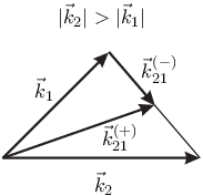
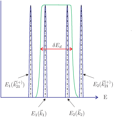
Figure 2: For |k→2|>|k→1||\vec{k}_{2}|>|\vec{k}_{1}| (left) the interference term has a periodic time–dependence with a frequency ω21\omega_{21} due to the relation E1​(k→1)<E1​(k→21(+))<E2​(k→21(+))<E2​(k→2)E_{1}(\vec{k}_{1})<E_{1}(\vec{k}^{(+)}_{21})<E_{2}(\vec{k}^{(+)}_{21})<E_{2}(\vec{k}_{2}) (right) with k→21(+)=(k→2+k→1)/2\vec{k}^{(+)}_{21}=(\vec{k}_{2}+\vec{k}_{1})/2.
Refer to caption
Refer to caption
Figure 3: For |k→2|<|k→1||\vec{k}_{2}|<|\vec{k}_{1}| (left) the interference term has a periodic time–dependence with a frequency Ω21>ω21\Omega_{21}>\omega_{21} due to the relation E1​(k→21(+))<E1​(k→1)<E2​(k→2)<E2​(k→21(+))E_{1}(\vec{k}^{(+)}_{21})<E_{1}(\vec{k}_{1})<E_{2}(\vec{k}_{2})<E_{2}(\vec{k}^{(+)}_{21}) (right) with k→21(+)=(k→2+k→1)/2\vec{k}^{(+)}_{21}=(\vec{k}_{2}+\vec{k}_{1})/2.

The region of variation of 3–momenta of massive neutrinos can be divided into two parts with the absolute values |k→2|>|k→1|\vec{k}_{2}|>|\vec{k}_{1} and |k→2|<|k→1||\vec{k}_{2}|<|\vec{k}_{1}|, respectively, and both cases lead to totally different modulation frequencies of the interference term.

For |k→2|>|k→1|\vec{k}_{2}|>|\vec{k}_{1}, the energies E1​(k→1)E_{1}(\vec{k}_{1}), E1​(k→21)E_{1}(\vec{k}_{21}), E2​(k→21)E_{2}(\vec{k}_{21}) and E2​(k→2)E_{2}(\vec{k}_{2}) satisfy the inequality: E1​(k→1)<E1​(k→21)<E2​(k→21)<E2​(k→2)E_{1}(\vec{k}_{1})<E_{1}(\vec{k}_{21})<E_{2}(\vec{k}_{21})<E_{2}(\vec{k}_{2}) as it shown in Fig. 2. The deviations as indicated in Fig. 2 are of order of O⁡(1/δ)O(1/\delta). Indeed, for sufficiently large δ\delta, that has been already assumed above for the calculation the rate of neutrino spectrum Eq.(10) and Eq.(11), due to the function e−δ2​(k→21(−))2e^{\,-\,\delta^{2}(\vec{k}^{(-)}_{21})^{2}} the region of the 3–momenta of massive neutrinos is constrained by k→2∼k→1\vec{k}_{2}\sim\vec{k}_{1}. The allowed region of deviations is of order of |k→21(−)|∼1/δ|\vec{k}^{(-)}_{21}|\sim 1/\delta. For these momenta the energies of neutrino mass–eigenstates obey the obvious relation E2​(k→2)≃E1​(k→1)≫|k→21(−)|∼1/δE_{2}(\vec{k}_{2})\simeq E_{1}(\vec{k}_{1})\gg|\vec{k}^{(-)}_{21}|\sim 1/\delta. Making the expansions of the energies of massive neutrinos in powers of k→21(−)\vec{k}^{(-)}_{21} and keeping only the first order contributions we get E2​(k→21(+))=E2​(k→2)−Δ​ℰ2E_{2}(\vec{k}^{(+)}_{21})=E_{2}(\vec{k}_{2})-\Delta{\cal E}_{2} and E1​(k→21(+))=E1​(k→1)+Δ​ℰ1E_{1}(\vec{k}^{(+)}_{21})=E_{1}(\vec{k}_{1})+\Delta{\cal E}_{1}, where we have denoted Δ​ℰ2=k→2⋅k→21(−)/E2​(k→2)\Delta{\cal E}_{2}=\vec{k}_{2}\cdot\vec{k}^{(-)}_{21}/E_{2}(\vec{k}_{2}) and Δ​ℰ1=k→1⋅k→21(−)/E1​(k→1)\Delta{\cal E}_{1}=\vec{k}_{1}\cdot\vec{k}^{(-)}_{21}/E_{1}(\vec{k}_{1}). Without loss of generality we can set Δ​ℰ2≃Δ​ℰ1≃Δ​ℰ\Delta{\cal E}_{2}\simeq\Delta{\cal E}_{1}\simeq\Delta{\cal E}, where |Δ​ℰ|=O⁡(1/δ)|\Delta{\cal E}|=O(1/\delta) and E2​(k→2)≃E1​(k→1)≫|Δ​ℰ|=O⁡(1/δ)E_{2}(\vec{k}_{2})\simeq E_{1}(\vec{k}_{1})\gg|\Delta{\cal E}|=O(1/\delta). This shows that the deviations of E2​(k→21(+))E_{2}(\vec{k}^{(+)}_{21}) and E1​(k→21(+))E_{1}(\vec{k}^{(+)}_{21}) from E2​(k→2)E_{2}(\vec{k}_{2}) and E1​(k→1)E_{1}(\vec{k}_{1}), respectively, are of order of O⁡(1/δ)O(1/\delta) and the interference term should have a periodic time dependence with a period ω21\omega_{21}.

In the region |k→2|>|k→1||\vec{k}_{2}|>|\vec{k}_{1}| of 3–momenta of massive neutrinos the calculation of the periodic term runs as follows

cos⁡((E2​(k→21(+))−E1​(k→21(+)))​t)⟹1/δ\displaystyle\cos((E_{2}(\vec{k}^{(+)}_{21})-E_{1}(\vec{k}^{(+)}_{21}))t)\stackrel{{\scriptstyle 1/\delta}}{{\Longrightarrow}}
⟹1/δcos⁡((E2​(k→2)−E1​(k→1))​t)=cos⁡(ω21​t),\displaystyle\stackrel{{\scriptstyle 1/\delta}}{{\Longrightarrow}}\cos((E_{2}(\vec{k}_{2})-E_{1}(\vec{k}_{1}))t)=\cos(\omega_{21}t), (16)

where we have used the on–shell relations between neutrino energies and momenta only for the expansions E2​(k→21(+))=E2​(k→2)−Δ​ℰ=E2​(k→2)−O⁡(1/δ)E_{2}(\vec{k}^{(+)}_{21})=E_{2}(\vec{k}_{2})-\Delta{\cal E}=E_{2}(\vec{k}_{2})-O(1/\delta) and E1​(k→21(+))=E1​(k→1)+Δ​ℰ=E1​(k→1)+O⁡(1/δ)E_{1}(\vec{k}^{(+)}_{21})=E_{1}(\vec{k}_{1})+\Delta{\cal E}=E_{1}(\vec{k}_{1})+O(1/\delta) but not for the energy difference. This gives E2​(k→21(+))−E1​(k→21(+))=E2​(k→2)−E1​(k→1)−2​Δ​ℰ=ω21−O⁡(2/δ)E_{2}(\vec{k}^{(+)}_{21})-E_{1}(\vec{k}^{(+)}_{21})=E_{2}(\vec{k}_{2})-E_{1}(\vec{k}_{1})-2\Delta{\cal E}=\omega_{21}-O(2/\delta). As a result the validity of the interference term to have a frequency ω21\omega_{21} should be confirmed by the inequality ω21≫2/δ\omega_{21}\gg 2/\delta, which can be always satisfied for the sufficiently large δ\delta.

In turn, for |k→2|<|k→1||\vec{k}_{2}|<|\vec{k}_{1}| the energies E1​(k→21(+))E_{1}(\vec{k}^{(+)}_{21}), E1​(k→1)E_{1}(\vec{k}_{1}), E2​(k→2)E_{2}(\vec{k}_{2}) and E2​(k→21(+))E_{2}(\vec{k}^{(+)}_{21}) satisfy the inequality: E1​(k→21(+))<E1​(k→1)<E2​(k→2)<E2​(k→21(+))E_{1}(\vec{k}^{(+)}_{21})<E_{1}(\vec{k}_{1})<E_{2}(\vec{k}_{2})<E_{2}(\vec{k}^{(+)}_{21}) as it shown in Fig. 3. In this case a periodic time–dependence of the interference term can be defined by the frequency, which is greater than ω21\omega_{21}.

In order to take into account both frequencies of the periodic time-dependence of the interference term we introduce the function

ρ⁡(k→2,k→1)\displaystyle\rho(\vec{k}_{2},\vec{k}_{1}) =\displaystyle= θ⁡(|k→2|−|k→1|)​ρ′​(k→2,k→1)\displaystyle\theta(|\vec{k}_{2}|-|\vec{k}_{1}|)\,\rho^{\prime}(\vec{k}_{2},\vec{k}_{1}) (17)
+\displaystyle+ θ⁡(|k→1|−|k→2|)​ρ′′​(k→2,k→1),\displaystyle\theta(|\vec{k}_{1}|-|\vec{k}_{2}|)\,\rho^{\prime\prime}(\vec{k}_{2},\vec{k}_{1}),

having a meaning of the probability density for neutrino mass–eigenstates ν2\nu_{2} and ν1\nu_{1} to have 3–momenta k→2\vec{k}_{2} and k→1\vec{k}_{1}, respectively. The Heaviside step functions θ⁡(|k→2|−|k→1|)\theta(|\vec{k}_{2}|-|\vec{k}_{1}|) and θ⁡(|k→1|−|k→2|)\theta(|\vec{k}_{1}|-|\vec{k}_{2}|) take into account two possibilities |k→2|>|k→1||\vec{k}_{2}|>|\vec{k}_{1}| and |k→2|<|k→1||\vec{k}_{2}|<|\vec{k}_{1}| for the 3–momenta of neutrino mass–eigenstates shown in Fig. 2 and Fig. 3.

The contribution of the interference term λE​C(2)​(t)\lambda^{(2)}_{EC}(t) to the E​CEC–decay rate we define as follows

λE​C(2)​(t)=limε→01(π​δ2)3/2​∫d​Nνe(2)​(t)d​t\displaystyle\lambda^{(2)}_{EC}(t)=\lim_{\varepsilon\to 0}\frac{1}{(\pi\delta^{2})^{3/2}}\int\frac{dN^{(2)}_{\nu_{e}}(t)}{dt}
×ρ⁡(k→2,k→1)​d3​k1(2​π)3​2​E1​(k→1)​d3​k2(2​π)3​2​E2​(k→2).\displaystyle\times\,\rho(\vec{k}_{2},\vec{k}_{1})\,\frac{d^{3}k_{1}}{(2\pi)^{3}2E_{1}(\vec{k}_{1})}\frac{d^{3}k_{2}}{(2\pi)^{3}2E_{2}(\vec{k}_{2})}. (18)

Substituting Eq.(17) into Eq.(18) we get

λE​C(2)​(t)=λE​C(2)′​(t)+λE​C(2)′′​(t),\displaystyle\lambda^{(2)}_{EC}(t)=\lambda^{(2)^{\prime}}_{EC}(t)+\lambda^{(2)^{\prime\prime}}_{EC}(t), (19)

where λE​C(2)′​(t)\lambda^{(2)^{\prime}}_{EC}(t) and λE​C(2)′′​(t)\lambda^{(2)^{\prime\prime}}_{EC}(t) are determined by the contributions of the regions |k→2|>|k→1||\vec{k}_{2}|>|\vec{k}_{1}| and |k→2|<|k→1||\vec{k}_{2}|<|\vec{k}_{1}|, respectively. They are given by the following momentum integrals

λE​C(2)′​(t)=limε→032​F+1​|ℳGT|2​|⟨ψ1​s(Z)⟩|2​12​sin⁡2​θ12\displaystyle\lambda^{(2)^{\prime}}_{EC}(t)=\lim_{\varepsilon\to 0}\frac{3}{2F+1}\,|{\cal M}_{\rm GT}|^{2}\,|\langle\psi^{(Z)}_{1s}\rangle|^{2}\,\frac{1}{2}\,\sin 2\theta_{12}
×∫d3​k1(2​π)3​2​E1​(k→1)​d3​k2(2​π)3​2​E2​(k→2)​θ​(|k→2|−|k→1|)\displaystyle\times\int\frac{d^{3}k_{1}}{(2\pi)^{3}2E_{1}(\vec{k}_{1})}\frac{d^{3}k_{2}}{(2\pi)^{3}2E_{2}(\vec{k}_{2})}\,\theta(|\vec{k}_{2}|-|\vec{k}_{1}|)
×ρ′​(k→2,k→1)​e−δ2​(k→21(−))2​E2​(k→21(+))​E1​(k→21(+))\displaystyle\times\,\rho^{\prime}(\vec{k}_{2},\vec{k}_{1})\,e^{\textstyle\,-\delta^{2}(\vec{k}^{(-)}_{21})^{2}}\,\sqrt{E_{2}(\vec{k}^{(+)}_{21})E_{1}(\vec{k}^{(+)}_{21})}
×[2​ε(Δ​E2​(k→21(+)))2+ε2+2​ε(Δ​E1​(k→21(+)))2+ε2]\displaystyle\times\,\Big[\frac{2\varepsilon}{(\Delta E_{2}(\vec{k}^{(+)}_{21}))^{2}+\varepsilon^{2}}+\frac{2\varepsilon}{(\Delta E_{1}(\vec{k}^{(+)}_{21}))^{2}+\varepsilon^{2}}\Big]
×cos⁡[(E2​(k→21(+))−E1​(k→21(+)))​t]​eε​t\displaystyle\times\,\cos\Big[\Big(E_{2}(\vec{k}^{(+)}_{21})-E_{1}(\vec{k}^{(+)}_{21})\Big)t\Big]\,e^{\textstyle\,\varepsilon t} (20)

and

λE​C(2)′′​(t)=limε→032​F+1​|ℳGT|2​|⟨ψ1​s(Z)⟩|2​12​sin⁡2​θ12\displaystyle\lambda^{(2)^{\prime\prime}}_{EC}(t)=\lim_{\varepsilon\to 0}\frac{3}{2F+1}\,|{\cal M}_{\rm GT}|^{2}\,|\langle\psi^{(Z)}_{1s}\rangle|^{2}\,\frac{1}{2}\,\sin 2\theta_{12}
×∫d3​k1(2​π)3​2​E1​(k→1)​d3​k2(2​π)3​2​E2​(k→2)​θ​(|k→1|−|k→2|)\displaystyle\times\int\frac{d^{3}k_{1}}{(2\pi)^{3}2E_{1}(\vec{k}_{1})}\frac{d^{3}k_{2}}{(2\pi)^{3}2E_{2}(\vec{k}_{2})}\,\theta(|\vec{k}_{1}|-|\vec{k}_{2}|)
×ρ′′​(k→2,k→1)​e−δ2​(k→21(−))2​E2​(k→21(+))​E1​(k→21(+))\displaystyle\times\,\rho^{\prime\prime}(\vec{k}_{2},\vec{k}_{1})\,e^{\textstyle\,-\delta^{2}(\vec{k}^{(-)}_{21})^{2}}\,\sqrt{E_{2}(\vec{k}^{(+)}_{21})E_{1}(\vec{k}^{(+)}_{21})}
×[2​ε(Δ​E2​(k→21(+)))2+ε2+2​ε(Δ​E1​(k→21(+)))2+ε2]\displaystyle\times\,\Big[\frac{2\varepsilon}{(\Delta E_{2}(\vec{k}^{(+)}_{21}))^{2}+\varepsilon^{2}}+\frac{2\varepsilon}{(\Delta E_{1}(\vec{k}^{(+)}_{21}))^{2}+\varepsilon^{2}}\Big]
×cos⁡[m22−m12E2​(k→21(+))+E1​(k→21(+))​t]​eε​t.\displaystyle\times\,\cos\Big[\frac{m^{2}_{2}-m^{2}_{1}}{E_{2}(\vec{k}^{(+)}_{21})+E_{1}(\vec{k}^{(+)}_{21})}t\Big]\,e^{\textstyle\,\varepsilon t}. (21)

According to Figs. 2 and 3, the frequencies in two integrals Eqs.(20) and (21) should be equal to ω21\omega_{21} and Ω21\Omega_{21}, respectively.

Making expansions in powers of |k→21(−)|∼1/δ|\vec{k}^{(-)}_{21}|\sim 1/\delta 33 3 Formally this leads to the replacements Δ​E2​(k→21(+))→Δ​E2​(k→2)\Delta E_{2}(\vec{k}^{(+)}_{21})\to\Delta E_{2}(\vec{k}_{2}), Δ​E1​(k→21(+))→Δ​E1​(k→1)\Delta E_{1}(\vec{k}^{(+)}_{21})\to\Delta E_{1}(\vec{k}_{1}), E2​(k→21(+))→E2​(k→2)E_{2}(\vec{k}^{(+)}_{21})\to E_{2}(\vec{k}_{2}) and E1​(k→21(+))→E1​(k→1)E_{1}(\vec{k}^{(+)}_{21})\to E_{1}(\vec{k}_{1}). and taking the limit ε→0\varepsilon\to 0 we reduce the r.h.s. of Eqs.(20) and (21) to the form

λE​C(2)′​(t)=32​F+1​|ℳGT|2​|⟨ψ1​s(Z)⟩|2​12​sin⁡2​θ12\displaystyle\lambda^{(2)^{\prime}}_{EC}(t)=\frac{3}{2F+1}\,|{\cal M}_{\rm GT}|^{2}\,|\langle\psi^{(Z)}_{1s}\rangle|^{2}\,\frac{1}{2}\,\sin 2\theta_{12}
×∫d3​k1(2​π)3​2​E1​(k→1)​d3​k2(2​π)3​2​E2​(k→2)​θ​(|k→2|−|k→1|)\displaystyle\times\int\frac{d^{3}k_{1}}{(2\pi)^{3}2E_{1}(\vec{k}_{1})}\frac{d^{3}k_{2}}{(2\pi)^{3}2E_{2}(\vec{k}_{2})}\,\theta(|\vec{k}_{2}|-|\vec{k}_{1}|)
×ρ′​(k→2,k→1)​e−δ2​(k→21(−))2​E2​(k→2)​E1​(k→1)\displaystyle\times\,\rho^{\prime}(\vec{k}_{2},\vec{k}_{1})\,e^{\textstyle\,-\delta^{2}(\vec{k}^{(-)}_{21})^{2}}\,\sqrt{E_{2}(\vec{k}_{2})E_{1}(\vec{k}_{1})}
×[2​π​δ​(Δ​E2​(k→2))+2​π​δ​(Δ​E1​(k→1))]\displaystyle\times\,\Big[2\pi\,\delta(\Delta E_{2}(\vec{k}_{2}))+2\pi\,\delta(\Delta E_{1}(\vec{k}_{1}))\Big]
×cos⁡[(E2​(k→2)−E1​(k→1))​t]\displaystyle\times\cos\Big[\Big(E_{2}(\vec{k}_{2})-E_{1}(\vec{k}_{1})\Big)t\Big] (22)

and

λE​C(2)′′​(t)=32​F+1​|ℳGT|2​|⟨ψ1​s(Z)⟩|2​12​sin⁡2​θ12\displaystyle\lambda^{(2)^{\prime\prime}}_{EC}(t)=\frac{3}{2F+1}\,|{\cal M}_{\rm GT}|^{2}\,|\langle\psi^{(Z)}_{1s}\rangle|^{2}\,\frac{1}{2}\,\sin 2\theta_{12}
×∫d3​k1(2​π)3​2​E1​(k→1)​d3​k2(2​π)3​2​E2​(k→2)​θ​(|k→1|−|k→2|)\displaystyle\times\int\frac{d^{3}k_{1}}{(2\pi)^{3}2E_{1}(\vec{k}_{1})}\frac{d^{3}k_{2}}{(2\pi)^{3}2E_{2}(\vec{k}_{2})}\,\theta(|\vec{k}_{1}|-|\vec{k}_{2}|)
×ρ′′​(k→2,k→1)​e−δ2​(k→21(−))2​E2​(k→2)​E1​(k→1)\displaystyle\times\,\rho^{\prime\prime}(\vec{k}_{2},\vec{k}_{1})\,e^{\textstyle\,-\delta^{2}(\vec{k}^{(-)}_{21})^{2}}\sqrt{E_{2}(\vec{k}_{2})E_{1}(\vec{k}_{1})}
×[2​π​δ​(Δ​E2​(k→2))+2​π​δ​(Δ​E1​(k→1))]\displaystyle\times\,\Big[2\pi\,\delta(\Delta E_{2}(\vec{k}_{2}))+2\pi\,\delta(\Delta E_{1}(\vec{k}_{1}))\Big]
×cos⁡[m22−m12E2​(k→2)+E1​(k→1)​t].\displaystyle\times\,\cos\Big[\frac{m^{2}_{2}-m^{2}_{1}}{E_{2}(\vec{k}_{2})+E_{1}(\vec{k}_{1})}\,t\Big]. (23)

By virtue of the δ\delta–functions δ⁡(Δ​E1​(k→1))\delta(\Delta E_{1}(\vec{k}_{1})) and δ⁡(Δ​E2​(k→2))\delta(\Delta E_{2}(\vec{k}_{2})) with arguments Δ​E1​(k→1)=Ed​(k→1)+E1​(k→1)−Mm\Delta E_{1}(\vec{k}_{1})=E_{d}(\vec{k}_{1})+E_{1}(\vec{k}_{1})-M_{m} and Δ​E2​(k→2)=Ed​(k→2)+E1​(k→2)−Mm\Delta E_{2}(\vec{k}_{2})=E_{d}(\vec{k}_{2})+E_{1}(\vec{k}_{2})-M_{m}, respectively, providing energy conservation in the E​CEC–decay channels m→d+ν1m\to d+\nu_{1} and m→d+ν2m\to d+\nu_{2}, and the function e−δ2​(k→21(−))2e^{\,-\delta^{2}(\vec{k}^{(-)}_{21})^{2}}, the frequencies of the periodic terms can be replaced by ω21\omega_{21} and Ω21\Omega_{21}, respectively. As a result the contribution of the interference term reads

λE​C(2)​(t)λE​C=aE​C​cos⁡(ω21​t)+a~E​C​cos⁡(Ω21​t),\displaystyle\frac{\lambda^{(2)}_{EC}(t)}{\lambda_{EC}}=a_{EC}\cos(\omega_{21}t)+\tilde{a}_{EC}\cos(\Omega_{21}t), (24)

where λE​C\lambda_{EC} is defined by Eq.(14). The amplitudes aE​Ca_{EC} and a~E​C\tilde{a}_{EC} are given by the integrals

aE​C=sin⁡2​θ12​2​π2QH2​∫d3​k1(2​π)3​2​E1​(k→1)​d3​k2(2​π)3​2​E2​(k→2)\displaystyle a_{EC}=\sin 2\theta_{12}\,\frac{2\pi^{2}}{Q^{2}_{\rm H}}\int\frac{d^{3}k_{1}}{(2\pi)^{3}2E_{1}(\vec{k}_{1})}\frac{d^{3}k_{2}}{(2\pi)^{3}2E_{2}(\vec{k}_{2})}
×ρ′​(k→2,k→1)​e−δ2​(k→21(−))2​E2​(k→2)​E1​(k→1)\displaystyle\times\,\rho^{\prime}(\vec{k}_{2},\vec{k}_{1})\,e^{\textstyle\,-\delta^{2}(\vec{k}^{(-)}_{21})^{2}}\sqrt{E_{2}(\vec{k}_{2})E_{1}(\vec{k}_{1})}
×[δ⁡(Δ​E2​(k→2))+δ⁡(Δ​E1​(k→1))]​θ​(|k→2|−|k→1|)\displaystyle\times\,\Big[\delta(\Delta E_{2}(\vec{k}_{2}))+\delta(\Delta E_{1}(\vec{k}_{1}))\Big]\,\theta(|\vec{k}_{2}|-|\vec{k}_{1}|) (25)

and

a~E​C=sin⁡2​θ12​2​π2QH2​∫d3​k1(2​π)3​2​E1​(k→1)​d3​k2(2​π)3​2​E2​(k→2)\displaystyle\tilde{a}_{EC}=\sin 2\theta_{12}\,\frac{2\pi^{2}}{Q^{2}_{\rm H}}\int\frac{d^{3}k_{1}}{(2\pi)^{3}2E_{1}(\vec{k}_{1})}\frac{d^{3}k_{2}}{(2\pi)^{3}2E_{2}(\vec{k}_{2})}
×ρ′′​(k→2,k→1)​e−δ2​(k→21(−))2​E2​(k→2)​E1​(k→1)\displaystyle\times\,\rho^{\prime\prime}(\vec{k}_{2},\vec{k}_{1})\,e^{\textstyle\,-\delta^{2}(\vec{k}^{(-)}_{21})^{2}}\sqrt{E_{2}(\vec{k}_{2})E_{1}(\vec{k}_{1})}
×[δ⁡(Δ​E2​(k→2))+δ⁡(Δ​E1​(k→1))]​θ​(|k→1|−|k→2|).\displaystyle\times\,\Big[\delta(\Delta E_{2}(\vec{k}_{2}))+\delta(\Delta E_{1}(\vec{k}_{1}))\Big]\,\theta(|\vec{k}_{1}|-|\vec{k}_{2}|). (26)

The amplitudes of the periodic functions, depending on the mixing angle θ12\theta_{12} and the parameter δ\delta, are considered as empirical parameters determined by the experiment.

We would like to emphasize that due to non–conservation of 3–momenta the massive neutrinos are off–shell. This means that on–shell relations Ej​(p→)=(p→ 2+mj2)1/2E_{j}(\vec{p}\,)=(\vec{p}^{\;2}+m^{2}_{j})^{1/2} between energies Ej​(p→)E_{j}(\vec{p}\,) and 3-momenta p→=k→j\vec{p}=\vec{k}_{j} or p→=k→i​j(+)\vec{p}=\vec{k}^{(+)}_{ij} are only approximate. This results in some constraints on the use of on–shell relations between energies and momenta. Indeed, for the correct calculation of the periodic time–dependence of the E​CEC–decay rate in the momentum integrals Eqs.(20)–(26) one cannot use on–shell relations between energies and momenta of massive neutrinos for the analysis of the differences of neutrino energies and momenta due to substantial sensitivity of these differences to the off–shell and on–shell states. As we have shown above (see Eq.(15) and a discussion below), the use of the on–shell relations between the energies E2​(k→21(+))E_{2}(\vec{k}^{(+)}_{21}) and E1​(k→21(+))E_{1}(\vec{k}^{(+)}_{21}) and the momentum k→21(+)\vec{k}^{(+)}_{21} leads to the missing of the frequency ω21\omega_{21} (see [17]).

Time–dependent E​CEC–decay rates of H–like heavy ions

Taking into account the contribution of the interference term, the total E​CEC–decay rate we get in the form

λE​C​(t)λE​C=1+aE​C​cos⁡(ω21​t)+a~E​C​cos⁡(Ω21​t).\displaystyle\frac{\lambda_{EC}(t)}{\lambda_{EC}}=1+a_{EC}\cos(\omega_{21}t)+\tilde{a}_{EC}\cos(\Omega_{21}t). (27)

The E​CEC–decay rate Eq.(27) contains two periodic terms. In the laboratory frame the periods are equal to

TE​C=2​π​γω21,Tg=2​π​γΩ21,\displaystyle T_{EC}=\frac{2\pi\gamma}{\omega_{21}}\quad,\quad T_{g}=\frac{2\pi\gamma}{\Omega_{21}}, (28)

where γ=1.43\gamma=1.43 is the Lorentz factor of the motion of mother ions in the laboratory frame [4]. We identify TE​C=2​π​γ/ω21∼MmT_{EC}=2\pi\gamma/\omega_{21}\sim M_{m} with the experimental period of the time–modulation TE​C=7.06​(8)​sT_{EC}=7.06(8)\,{\rm s}, because it is shown experimentally that the period of the time–modulation does not depend on the QQ–value of the weak transition. For the E​CEC–decay of the H–like Pm60+142{{}^{142}}{\rm Pm}^{60+} ion with QH≃4827​keVQ_{\rm H}\simeq 4827\,{\rm keV} the period of modulation TE​C=7.10​(22)​sT_{EC}=7.10(22)\,{\rm s} is equal to TE​C=7.06​(8)​sT_{EC}=7.06(8)\,{\rm s} of the H–like Pr58+140{{}^{140}}{\rm Pr}^{58+} ion within the experimental error bars. Since the mass difference of the H–like ions Pm60+142{{}^{142}}{\rm Pm}^{60+} and Pr58+140{{}^{140}}{\rm Pr}^{58+} is small we expect only small differences in the periods of the time–modulation as shown by the experiment.

Thus, for TE​C=7.06​(8)​sT_{EC}=7.06(8)\,{\rm s} we get (Δ​m212)GSI=2.22​(3)×10−4​eV2(\Delta m^{2}_{21})_{\rm GSI}=2.22(3)\times 10^{-4}\,{\rm eV^{2}} (see also [18]). The value (Δ​m212)GSI=2.22​(3)×10−4​eV2(\Delta m^{2}_{21})_{\rm GSI}=2.22(3)\times 10^{-4}\,{\rm eV^{2}} is by a factor of 2.75 larger than (Δ​m212)KamLAND=0.80−0.05+0.06×10⁻⁴​eV2(\Delta m^{2}_{21})_{\rm KamLAND}=0.80^{+0.06}_{-0.05}\times 10^{-4}\,{\rm eV^{2}}, obtained as a best–fit of the global analysis of the solar–neutrino and KamLAND experimental data [5, 9].

For (Δ​m212)GSI=2.22​(3)×10−4​eV2(\Delta m^{2}_{21})_{\rm GSI}=2.22(3)\times 10^{-4}\,{\rm eV^{2}} we get Tg≃1.8×10⁻⁴​sT_{g}\simeq 1.8\times 10^{-4}\,{\rm s}. These fast oscillations, averaged over the experimental time resolution Δ​T=0.32​s\Delta T=0.32\,{\rm s} [4], are not observable. As a result the time–dependent E​CEC–decay rate Eq.(27) is given only by the low frequency term

λE​C​(t)=λE​C​(1+aE​C​cos⁡(ωE​C​t)),\displaystyle\lambda_{EC}(t)=\lambda_{EC}\,(1+a_{EC}\cos(\omega_{EC}t)), (29)

where ωE​C=ω21=2​π/TE​C\omega_{EC}=\omega_{21}=2\pi/T_{EC} and the amplitude aE​Ca_{EC} is defined by Eq.(25).

Discussion and summary

We have shown that the experimental data on the time–modulation of the rate of the number of daughter ions Ce58+140{{}^{140}}{\rm Ce}^{58+}, observed in the E​CEC–decay of the H–like ion Pr58+140{{}^{140}}{\rm Pr}^{58+} [4], can be explained by the neutrino mass differences. However, the difference of squared neutrino masses (Δ​m212)GSI=2.22​(3)×10−4​eV2(\Delta m^{2}_{21})_{\rm GSI}=2.22(3)\times 10^{-4}\,{\rm eV^{2}}, derived from the period TE​C=7.06​(8)​sT_{EC}=7.06(8)\,{\rm s} of the rate of the number of daughter ions Ce58+140{{}^{140}}{\rm Ce}^{58+}, is 2.75 times larger than the value measured by KamLAND [5]. A solution of this problem in terms of neutrino mass corrections, induced by the interaction of massive neutrinos with a strong Coulomb field of the daughter ion through virtual ℓ−​W+\ell^{-}W^{+} pair creation, is proposed in [15].

In summary we argue that the mechanism of the time–dependence of the E​CEC–decay rates of the H–like heavy ions bears similarity with quantum beats of atomic transitions [6], as the E​CEC–decays are the transitions of the initial state |m⟩|m\rangle into the final state |d​νe⟩|d\nu_{e}\rangle, where the electron neutrino is the coherent state of two massive neutrinos with energy difference ω21\omega_{21}. A sophisticated calculation of the interference term shows also the existence of a periodic time–dependence with a frequency Ω21≫ω21\Omega_{21}\gg\omega_{21}. In order to take into account the contributions of two possible frequencies of the periodic time–dependence of the interference term we have introduced the probability density ρ⁡(k→2,k→1)\rho(\vec{k}_{2},\vec{k}_{1}) for neutrino mass–eigenstates ν2\nu_{2} and ν1\nu_{1} to get 3–momenta k→2\vec{k}_{2} and k→1\vec{k}_{1}, respectively. The calculation of the function ρ⁡(k→2,k→1)\rho(\vec{k}_{2},\vec{k}_{1}) is rather hard problem. We can only argue that in the massless limit it should be equal to

ρ⁡(k→2,k→1)=2​Eν​(k→1)​Eν​(k→2)​(2​π)3​δ(3)​(k→2−k→1),\displaystyle\rho(\vec{k}_{2},\vec{k}_{1})=2\sqrt{E_{\nu}(\vec{k}_{1})E_{\nu}(\vec{k}_{2})}(2\pi)^{3}\delta^{(3)}(\vec{k}_{2}-\vec{k}_{1}),

which is required by the necessity to retain the meanvalue of the E​CEC–decay rate λE​C\lambda_{EC}.

The necessary condition for the appearance of the interference term in the E​CEC–decay rate is the overlap of the energy levels of neutrino mass–eigenstates. Non–conservation of 3–momenta of neutrino mass–eigenstates provides a possibility to place the interference term of the E​CEC–decay rate in the energy region of the diagonal term, defining the meanvalue of the E​CEC–decay rate λE​C\lambda_{EC}. A validity of such a transformation is supported by the constraint ω21=Δ​m212/2​Mm≫2/δ\omega_{21}=\Delta m^{2}_{21}/2M_{m}\gg 2/\delta, which makes impossible the limit Δ​m212→0\Delta m^{2}_{21}\to 0 in the argument of the interference term, where the terms of order O⁡(1/δ)O(1/\delta) are dropped with respect to Δ​m212/4​Mm\Delta m^{2}_{21}/4M_{m}. This means that in the interference term of the E​CEC–decay rate Eq.(29) one cannot set Δ​m212→0\Delta m^{2}_{21}\to 0 in order to reduce the time–dependent E​CEC–decay rate to the E​CEC–decay rate λE​C\lambda_{EC} given by Eq.(14). A correct reduction of λE​C​(t)\lambda_{EC}(t) to λE​C\lambda_{EC} can be carried out only by means of the averaging over time ⟨λE​C​(t)⟩=λE​C\langle\lambda_{EC}(t)\rangle=\lambda_{EC}. In spite of momentum non–conservation, energy of the E​CEC–decay is conserved in our approach. This is required by Fermi Golden Rule [14].

We acknowledge many fruitful discussions with T. Ericson, M. Faber, M. Kleber, F. Bosch, Yu. A. Litvinov, H. Lipkin, E. L. Kryshen, M. Pitschmann, N. I. Troitskaya and K. Yazaki in the course of this work. We are greatful to M. Gell–Mann and W. Weise for discussions and encouraging comments. We thank H. Kleinert for the recommendation to use the ε→0\varepsilon\to 0 regularization for the calculation of the integral over time in Eq.(5) and A. Gal for calling our attention to the period TgT_{g}.

This research was partly supported by the DFG cluster of excellence ”Origin and Structure of the Universe”.

References

  • [1] Yu. A. Litvinov et al. (the GSI Collaboration), Phys. Rev. Lett. 99, 262501 (2008).
  • [2] A. N. Ivanov et al., Phys. Rev. C 78, 025503 (2008); arXiv: 0711.3184 [nucl–th].
  • [3] W. Bambynek et al., Rev. Mod. Phys. 49 (1977) 77.
  • [4] Yu. A. Litvinov et al. (the GSI Collaboration), Phys. Lett. B 664, 162 (2008).
  • [5] W.–M. Yao et al., J. Phys. G 33, 1 (2006).
  • [6] W. W. Chow et al. Phys. Rev. A 11, 1380 (1975).
  • [7] L. Stodolsky, Phys. Rev. D 58, 036006 (1998); H. Lipkin, Phys. Lett. B 642, 366 (2006).
  • [8] W. Grimus, Lect. Notes Phys. 629, 169 (2004).
  • [9] G. Fogli et al., Prog. Part. Nucl. Phys. 57, 71, 742 (2006).
  • [10] R. P. Feynman et al., in The Feynman lectures on physics, Quantum mechanics, Addison–Wesley, Massachusetts, 1966.
  • [11] A. N. Ivanov et al., arXiv: 0807.2750 [nucl–th].
  • [12] C. Giunti, Phys. Lett. B 665, 92 (2005).
  • [13] H. Kienert et al., arXiv: 0808.2389 [hep–ph].
  • [14] W. Greiner, in Quantum mechanics, an Introduction, Springer–Verlag, Berlin, 2001.
  • [15] A. N. Ivanov et al., arXiv: 0804.1311 [nucl–th].
  • [16] C. Giunti, C. W. Kim, Phys. Rev. C 58, 017301 (1998).
  • [17] A. Gal, arXiv: 0809.1213 [nucl–th].
  • [18] H. Kleinert, P. Kienle, arXiv: 0803.2938 [nucl–th]; H. Lipkin, arXiv: 0805.0435 [hep-ph].