CESAM: a free code for stellar evolution calculations

Journal: Astrophysics and Space Science (CoRoT/ESTA Volume)

P. Morel Affiliation: Cassiopée, URA CNRS 1362, Observatoire de la Côte d’Azur, Nice, France
Tel.: +033-492003039
Fax: +033-492003121 E-mail: Pierre.Morel@obs-nice.fr Y. Lebreton Affiliation: Observatoire de Paris, GEPI, CNRS UMR 8111, 5 Place Janssen, 92195 Meudon, France E-mail: Yveline.Lebreton@obspm.fr

Received date / accepted date

Abstract

The cesam code is a consistent set of programs and routines which perform calculations of 1D quasi-hydrostatic stellar evolution including microscopic diffusion of chemical species and diffusion of angular momentum. The solution of the quasi-static equilibrium is performed by a collocation method based on piecewise polynomials approximations projected on a B-spline basis; that allows stable and robust calculations, and the exact restitution of the solution, not only at grid points, even for the discontinuous variables. Other advantages are the monitoring by only one parameter of the accuracy and its improvement by super-convergence. An automatic mesh refinement has been designed for adjusting the localisations of grid points according to the changes of unknowns. For standard models, the evolution of the chemical composition is solved by stiffly stable schemes of orders up to four; in the convection zones mixing and evolution of chemical are simultaneous. The solution of the diffusion equation employs the Galerkin finite elements scheme; the mixing of chemicals is then performed by a strong turbulent diffusion. A precise restoration of the atmosphere is allowed for.

Keywords:

Methods: numerical sun: evolution sun: interior stars: evolution stars: interior

pacs

97.10.Cv 97.10.Sj 95.75.Pq

1 Introduction to CESAM.

Within the limitations due to electronic degeneracy, cesam allows the computation of the quasi-static evolution of stellar models as long as the assumption of quasi-static equilibrium remains valid, that is to say, until the exhaustion of oxygen in the core. The modular structure of cesam facilitates the choices among several physical formalisms, for equation of state (hereafter EOS), convection, opacities, diffusion coefficients, etc… Many nuclear networks and initial mixtures are available which allow to optimise the physical description according to the kind of model and evolutionary phase of interest. Mass loss and infall of planetoids are also implemented.

The available packages.

Earlier versions, cesam2-3-4, were programmed in F77 and cesam5 in F90. Though obsolete, cesam4 and cesam5 are available at:

http://www.obs-nice.fr/morel/CESAM

In the early 2000’s, cesam was re-programmed in F95 and named cesam2k. Three versions are now available:

•

The “fixed version” and the “fixed COROT version”, limited to 3 $\alpha$ burning, available respectively at:

http://www.obs-nice.fr/cesam/

http://perso.obspm.fr/ $\sim$ lebreton/Modeles/CESAM.html
•

The “ $\beta$ version” more complete, not fixed, still in development (not free of bugs) is hereafter signalled by the flag $(\beta)$ . It includes evolution up to oxygen burning, diffusion of the angular momentum and other developments of minor importance. It is available at:

http://www.obs-nice.fr/morel/CESAM

Each package contains five directories and two files:

•

“SOURCE”, contains the fortran sources.
•

“EXPLOIT”, contains programs to exploit the models and examples of input files.
•

“SUN_STAR_DATA”, contains physical data and programs for their implementation.
•

“TESTS”, contains programs performing various checks.
•

“SCRIPTS”, contains scripts to be used for the implantation and operating, and a MAKEFILE.
•

“aide_mem2k.ps”, a short guide of directions for use, the “aide-mémoire” (hereafter Paper 2).
•

“cesam2k.ps”, a complete description of the numerical aspects and physics implemented, the “notice” (hereafter Paper 3).

The source is structured in 14 modules: numerical routines, opacities, convection, etc. All the F95 routines of the source are compiled once. The requirements for the calculations are read in external files to be supplied by the user. The run is interactive. Messages displayed in French, or in English, allow the control of calculations. The extent of convection zones, a H--R diagram, and the profiles of temperature, pressure, luminosity and abundances are displayed¹¹ 1 Use of the PGPLOT package. on line. cesam has been especially designed to facilitate the implementation of various physical constants, opacities, EOS, atmosphere, nuclear networks etc. So, its overall structure is separated in two spaces:

1.

A “physical space” where the coefficients of the differential equations are written in a form close to their physical formalism.
2.

A “numerical space” where the differential equations are formally solved.

Therefore cesam allows to implement physical processes, and physical data, without any knowledge of numerical methods involved for the solution of the equations. For the physics, the use of generic routines makes the reading of the algorithms easier.

Units and values of physical constants.

cesam uses cgs units except for the mass, radius and luminosity expressed in solar units. Two sets of fundamental constants are implemented which correspond to widely used values (Clayton, 1968; Christensen-Dalsgaard, 1988; Lide et al., 1994; Cox, 2000). For each calculation, one of these sets is chosen as the unique source of fundamental constants. Other constants are initialised locally, e.g. the mass excesses, in the routine performing the calculations of thermonuclear reaction rates.

Input files.

Very often only the “input data file” (hereafter IDF) is needed. It is read at the onset of the run and collects all the requirements needed for the calculations:

•

physical parameters: mass, chemical composition, mixing-length parameter, etc.
•

numerical parameters: maximum number of shells, kind of precision, etc.
•

criteria for halting the computations: age to be reached, value of the hydrogen abundance at centre, etc.
•

names and locations of the external data files containing the data of the tabulated EOS and opacity, names of the physical routines to be used, name of the model, of the set of units to be used, etc.

The other input files have only specific functions, among them the most useful are:

•

“mixture” allows the use of an initial mixture not implemented in cesam.
•

“modif_mix” allows to modify the abundances of some species in a mixture already implemented.
•

“reglages” allows to personalise the kind of precision to be used (see below).
•

“planet” contains the characteristics of infall of planetoids.
•

“rap_iso” allows to modify the isotopic ratios.
•

“vent” defines the chemical composition of the wind when it differs from the atmosphere composition.
•

“zoom” allows to fit the resolution of the display for the plot on line.
•

“langue” allows to have the messages in English.

The meaning of all items are explained in Paper 2. Examples of files are given in the directory EXPLOIT.

Output files.

At the end of each time step, a “return binary file” (hereafter RBF) is created. It contains all the data needed to initialise or pursue a computation. There is the possibility, either to save all RBF, or to keep only the last RBF created. On request, “output data files” (hereafter ODF) are created. Three ODF are designed for adiabatic, non adiabatic and inversion asteroseismic investigations. These ODF also serve as input for some programs of the directory EXPLOIT. An ODF concerns the diffusion of the angular momentum ( $\beta$ ). All items of output files are detailed in Paper 2. It is also possible to create personalised ODF.

The kinds of precision.

To optimise the calculations, sets of parameters, named “réglages”, are fixed according to the kind of models to be calculated and to their subsequent use. The most useful réglages are:

•

“realistic precision” for standard evolutions.
•

“super precision” used when a high level accuracy is needed.
•

“solar accuracy”, close to super precision, but especially designed for seismological investigations; the number of shells of the last model is increased up to its maximal value.
•

“corot”, close to super precision, but especially designed for investigations connected to CoRot.
•

“advanced”, for the computation of early type star models evolved up to the oxygen burning.
•

“normal precision”, for exploratory work.
•

“low mass”, for the computation of late type star models.
•

“reglages”, in that case, the parameters, designed by the user, are read on an input file named “reglages”.

The larger the expected accuracy, the larger the computational expense.

Operating data and programs.

The directory EXPLOIT contains:

•

examples of input files as IDF, “reglages”, “planet”, “modif_mix”, etc.
•

ASCII files of preliminary models for the initialisations of PMS and ZAMS models.
•

miscellaneous programs to make plots of the chemical composition profile, or an extension of the grid on a given set of radius, or create the IDF for solar calibration, etc.

The flow chart of cesam is described in Sect. 2. As the numerical features are detailed in the appendix of Morel (1997)²² 2 Only available on electronic form. (hereafter Paper I) they are only succinctly recalled in Sect. 3, except for the automatic allocation of mesh points described in Sect. 3.1. The restitution of the atmosphere is outlined in Sect. 4. The algorithms performing the temporal evolution are described in Sect. 5. The nuclear network is detailed in Sect. 6 and the implementation of the rotation is described in Sect. 7. The various formalisms of convection implanted in cesam are described in Sect. 9. Mass loss formalisms and infall of planetoids are described in Sect. 8. EOS and opacities data available are listed in Sect. 10.

2 The flow chart.

Initialisations.

At the onset of the run, the IDF is read. Chemical composition is initialised according to the initial mixture and to the isotopes used by the chosen nuclear network. Then, using fit-formulas (see Sect. 6.1), the thermonuclear reactions rates are tabulated on a relevant interval of temperatures³³ 3 The errors introduced by these interpolations remain within the error bars of the data.. Then, evolution begins:

•

either it starts from zero age on PMS or ZAMS: an initial model having the required specifications is deduced from a model taken from a RBF or from a model in ASCII chosen in the directory EXPLOIT.
•

or it pursues a previous calculation, then the input is one RBF of the evolution going on.

The evolution.

The number of shells is updated as explained in Sect. 3.1. Then, taking possible overshooting into account, the limits between radiative zones and convective mixed zones (hereafter LMR) are localised. The angular velocity ( $\beta$ ) and the chemical composition are then updated. In fine, the equations of quasi-static equilibrium for the interior and the atmosphere are solved. The process is repeated until convergence.

When the nuclear engine is at work, the time step control is first based on the local accuracy achieved for the numerical integration of species of relevant interest (see Sect. 6.2 and Sect. 6.3) and, second on a limitation of the relative changes of helium on the whole star. Otherwise, during the pre-main sequence, the limitation of the change of mechanical energy controls the time step. In case of divergence of any iterative algorithm the time step is halved.

Stop criteria.

According to flags, read in the IDF, the computations may be stopped:

•

when the expected age is reached.
•

when the central temperature reaches a given value.
•

as soon as the abundance of hydrogen at centre reaches a given value.
•

at the exhaustion of hydrogen at centre.
•

when the helium core reaches a given extent.
•

when the effective temperature crosses a given value.
•

at the ignition of the $3\alpha$ cycle.
•

at the ignition of the carbon cycle.
•

at the ignition of the oxygen cycle.

For most kinds of precision, the last time step is adjusted in order to fulfil the required stop condition.

3 Numerical methods.

Choice of variables.

For the numerical integration of the stellar structure equations, the Lagrangian form is the most convenient as the discretisation on mass is readily expressed. However, it presents a singularity at centre and the core needs to be integrated apart. The Eulerian form of the equations does not suffer from such inconvenience, but since the stellar radius varies with time, there is a free boundary (see Stoer & Bulirsch, 1979, par. 7.3). With the Lagrangian variables: $\mu\equiv M^{2/3}$ , $R^{2}$ , $L^{2/3}$ , the central singularity disappears (see 50, par. B1) and there is no need of a special treatment for the core ( $M$ is the mass, $L$ the luminosity and $R$ the radius). To be consistent, the chemical species are taken as functions of $M^{2/3}$ . The pressure, $P$ , and the temperature, $T$ , are expressed in logarithms, ( $\xi=\ln P$ , $\eta=\ln T$ ), on the ground that they change by more than six magnitudes from the centre to the atmosphere.

Solving the differential equations.

The unknowns are approached by piecewise polynomials of order defined according to the required accuracy; the mostly used are of order 1, i.e. linear piecewise, and of order 2, i.e. parabolic piecewise. For the stellar modelling, such a flexible representation is well adapted to the presence of discontinuities resulting from the mixing of the convection zones. For the calculations, the piecewise polynomials are projected on a local linear basis of normalised B-splines (De Boor, 1978; Schumaker, 1981). That allows to find back exactly the solution at any location. Moreover, B-splines basis are also used for solving:

•

the two points boundary initial value problems of the stellar structure and of the atmosphere by collocation (De Boor, 1978, ch. XV).
•

the diffusion equations of chemicals and angular momentum by finite elements (Quarteroni & Valli, 1994).

The linear systems involved by the resolution of implicit equations are band-diagonal.
However, due to the non-trivial and unfamiliar algebra of B-splines, the algorithms are much more elaborated than with the finite differences. Furthermore, efficient and stable algorithms have been constructed for integration, differentiation, integration of differential equations by collocation and for interpolation. In cesam the routines, especially constructed to manage the calculations with B-splines, are derived from the algorithms of Schumaker (1981, chap. 4). Details are given in 50.

3.1 Moving grid, mesh refinement and discontinuities tracking.

An automatic mesh refinement is implemented. At time $t$ , the locations of the $n(t)$ mesh points are set by fulfilling the condition that, from a grid point to the next, the jump of a strictly monotonous “repartition function”, $Q(\mu,t)$ , is equal to a “repartition constant” $C(t)$ (see Eggleton, 1971; Press et al., 1986, sect. 16.5). The locations of grid points, $\mu_{i},i=1,\ldots,n$ , known at the issue of the computations, satisfy:

Q(\mu_{i+1},t)-Q(\mu_{i},t)\equiv C(t),\quad i=1,\ldots,n-1.

(1)

The choice of $Q(\mu,t)$ is based on an a priori knowledge of the behaviour of the solution. For each $t$ , one defines an “index” function $q(\mu,t)$ mapping $[0,\mu_{\rm b}]$ on $[1,n]$ ; the index 1 (resp. $n$ ) corresponds to the centre and the index $n$ to the surface, i.e. $\mu_{\rm b}=M_{\rm ext}^{\frac{2}{3}}$ . Therefore, the integration is made on an equidistant grid. In terms of the derivative of $Q$ with respect to $q$ , Eq. (1) reads:

\left(\frac{\partial\psi}{\partial q}\right)_{t}=0,\ {\rm with}\ \psi(t)\equiv\left(\frac{\partial Q}{\partial q}\right)_{t}.

The change of variables $\mu\rightarrow q(\mu,t)$ :

\psi(t)=\theta\left(\frac{\partial\mu}{\partial q}\right)_{t},\ {\rm with}\ \theta(\mu,t)\equiv\left(\frac{\partial Q}{\partial\mu}\right)_{t}

is calculated from the analytic form of $Q(\mu,t)$ . There are two more unknowns: $\psi(t)$ and $\mu(q,t)$ ; they fulfil a system of differential equations of first order with boundary conditions:

\left(\frac{\partial\mu}{\partial q}\right)_{t}=\frac{\psi}{\theta},\ \left(\frac{\partial\psi}{\partial q}\right)_{t}=0,\ {\rm with}\ \left\{\begin{array}[]{l}q=1,\ \mu=0\\ q=n,\ \mu=\mu_{\rm b}.\end{array}\right.

The differential equations of internal structure and of atmosphere, written with respect to $q$ , are detailed in 50. The equations are then solved on an equidistant grid, that allows numerical optimisations.

Choice of $Q$ .

$Q$ should be a strictly monotonous, two times differentiable function as simple as possible. By experiments, it has been found that the most convenient compromise is:

Q=\Delta_{\xi}\xi+\Delta_{\eta}\eta+\Delta_{\mu}\mu,\ \Delta_{\xi}=\Delta_{\eta}=-1,\ \Delta_{\mu}=15.

where $\xi$ and $\eta$ have been defined above.

Mesh refinement.

The initial value of $C(t)$ is fixed according to the expected level of accuracy. Along the evolution, its value is kept within $\pm 2\%$ , of its initial value by increasing (or decreasing) the total number of shells.

Setting a grid point on a LMR.

At the limit between a mixed zone and a radiative one, there may be a singularity of chemicals. Therefore each LMR has to coincide precisely with a grid point. To do that cesam uses a weighted repartition function. On each side of a LMR, the weights are computed in such a way that they adjust locally the values of $C(t)$ to the amounts just needed for iteratively “pushing” the closest grid point on the limit. In most cases, including mixing, the distances from the LMR locations to the closest grid points are lower than a few per cents of the characteristic local grid size. The more well defined the location of the LMR, the most efficient the algorithm.

The grids.

cesam uses several grids for the B-splines representations of quasi-static variables, atmosphere and rotation variables. As it coincides with the adjustable grid of quasi-static variables, the Lagrangian grid used for the abundances of chemicals, is not fixed with respect to time. There is the possibility to use a “fixed grid”, to avoid the numerical diffusion resulting from the variable Lagrangian grid.

4 Atmosphere.

The atmosphere connects the convective optically thick outer part of the envelope to the optically thin interstellar medium. In the interior, the diffusion approximation (Kippenhahn & Weigert, 1991) is used to simplify the calculation of the radiative flux. In the outermost parts, this approximation is no longer valid, as soon as the Rosseland optical depth is lower than $\simeq 10$ : a special treatment is needed to restore the atmosphere.
cesam restores the atmosphere from a $T(\tau,T_{\rm eff},g)$ law here, $\tau$ is the Rosseland optical depth, $T_{\rm eff}$ the effective temperature and $g$ the gravity. The stellar radius, $R_{\star}$ , is defined as the bolometric one, i.e. the radius at the level where the local temperature is equal to $T_{\rm eff}$ (Morel et al., 1994). For genuine radiative $T(\tau)$ laws, whatever is $T_{\rm eff}$ , $\tau_{\star}$ is located at a fixed optical depth, e.g. $\tau_{\star}=2/3$ for the Eddington’s law. For more precise laws, the value of $\tau_{\star}$ is not fixed. Therefore, the location where $\tau_{\star}$ is defined is a free boundary.
As oscillation modes are reflected in the outermost parts of stars, the pressure, the temperature and their gradients should be continuous at the limit with the envelope. The continuity of the pressure gradient is trivially insured by the equation of quasi-static equilibrium verified on both sides of the limit. The continuity of the temperature gradient is more intricate to fulfil as the connection occurs in zones of convective instability. For the restoration of the atmosphere, the temperature gradient is derived from the $T(\tau)$ law itself. Fixing the gravity the $T(\tau)$ law is expressed as: $T^{4}=\frac{3}{4}T_{\rm eff}^{4}f(\tau)$ .

{\rm Using}\ d\tau=-\kappa\rho dr\ {\rm and}\ \nabla_{\rm rad}=\frac{3}{16\pi acG}\frac{P\kappa L}{MT^{4}},

after some calculations:

	$\displaystyle\nabla\equiv\frac{d\ln T}{d\ln P}=\frac{P\kappa}{T}\frac{{\rm d}T}{{\rm d}\tau}\frac{R^{2}}{GM}=$		(2)
	$\displaystyle\frac{3}{16\pi acG}\frac{P\kappa L_{\star}}{MT^{4}}\left(\frac{R}{R_{\star}}\right)^{2}\frac{{\rm d}f}{{\rm d}\tau}=\nabla_{\rm rad}\frac{L}{L_{\star}}\left(\frac{R}{R_{\star}}\right)^{2}\frac{{\rm d}f}{{\rm d}\tau}$

Here $\kappa$ is the Rosseland mean opacity, $\rho$ the density, $a$ the radiation constant, $G$ the gravitational constant, $L_{\star}$ the luminosity of the star, $c$ the speed of light and $\nabla_{\rm rad}$ the radiative gradient. In principle, the continuity is ensured when the same convection theory prevails on both sides. As in most cases the values differ, the continuity of the temperature gradient is insured by a weighted mean with respect to $\ln\tau$ .
Eq. (2) is no longer valid for a genuine radiative $T(\tau)$ law, as it ignores convection. In such a case, following the prescription of Henyey et al. (1965) , the temperature gradient in the convective atmosphere is computed with a modified radiative gradient:

\nabla_{\rm rad}^{*}=\nabla_{\rm rad}\frac{df}{d\tau}.

For a genuine radiative $T(\tau)$ law:

\lim_{\tau\gg 1}\frac{df}{d\tau}=1,

therefore, at the limit between the atmosphere and the envelope, the radiative gradient is continuous and consequently the convective temperature gradient.
The numerical integration of the differential equations fulfilled in the atmosphere is made by collocation, see 50 for details. The number of shells in the atmosphere is fixed from 50 to 100 according to the required level of accuracy.

5 Evolution of the internal structure.

Initial PMS model.

The energy source in an initial PMS model is only of gravitational origin. At the onset of the Hayashi track, the star is fully convective, therefore isentropic and chemically homogeneous. The energy equation is reduced as in Iben (1965):

\frac{\partial L}{\partial M}=\epsilon_{G}=-T\frac{\partial S}{\partial t}=c(t)T

(3)

where $c(t)$ is the “contraction constant”, and $S$ the entropy. Along the interval of time $\Delta t$ , the energy radiated equals the change of gravitational energy, therefore, at first order:

	$\displaystyle\frac{L(t)+L(t+\Delta t)}{2}\Delta t\sim\left(\frac{GM^{2}}{R(t+\Delta t)}-\frac{GM^{2}}{R(t)}\right)\ \Rightarrow$
	$\displaystyle\Delta t\sim\frac{2GM^{2}\left[R(t)-R(t+\Delta t)\right]}{(L(t)+L(t+\Delta t))R(t)R(t+\Delta t)}.$

here $R(t)$ is the stellar radius. An estimate of the initial time step is deduced from two models computed with Eq. (3), with close values of the contraction constant, $c(t)$ and $c(t+\Delta t)$ . cesam uses: $c(t+\Delta t)=1.1\times c(t)$ . With $c(t)=0.02$ cgs the temperature at centre is about $10^{5}$ K; it is ten times larger with $c(t)=0.00008$ cgs. Changes of the contraction constant allow to choose between different initial PMS models. Most of the PMS models can be initialised with a preliminary model in ASCII available in the directory EXPLOIT. cesam assumes that a PMS model becomes a ZAMS model as soon as the release of gravitational energy balances the thermonuclear nuclear one. Such a model is chemically inhomogeneous.

Initial homogeneous ZAMS model.

A model of ZAMS with homogeneous chemical composition is not a physical reality as the nuclear engine does not work at equilibrium. However, it is a very convenient short way as, after a few time steps, the model is very close to the model at the end of the PMS. Several ZAMS initial models in ASCII are available in the directory EXPLOIT.

6 Evolution of chemicals.

6.1 The nuclear networks.

At the onset of the computations, the abundances of chemicals are initialised according to the initial hydrogen and helium mass ratios and mixture. The initial abundance of each chemical species is split between its isotopes, according to the isotopic ratios of nuclides. Several mixtures are implemented, the most useful are: the Anders & Grevesse (1989) meteoritic mixture and the solar mixtures of Grevesse & Noels (1993) and Grevesse & Sauval (1998). If necessary an IDF allows to modify the initial abundances of specific species or to use a mixture not yet implemented.
Up to 16 nuclear networks are presently available. Hence, one can follow the evolution using only the chemical species and the thermonuclear reactions of interest.
The nuclear reaction rates are tabulated on relevant intervals of temperatures. The rates are computed using the formulas of Caughlan & Fowler (1988) or of NACRE compilations (Angulo et al., 1999). For solar models, the improved rates of Adelberger et al. (1998) are available. The weak screening of Salpeter (1961) and the weak and intermediate screenings of Mitler (1997) are available.

6.2 Evolution without diffusion.

The time scales involved in the temporal evolution of chemicals differ by a large number of magnitudes. From a mathematical point of view it is a stiff problem (Hairer & Wanner, 1991) and algorithms have been especially designed for it. Without microscopic diffusion, L-stable (Hairer & Wanner, 1991, par. 4.3) implicit Runge-Kutta schemes, are available for the chemical evolution.
In the radiative zones, the equations to be solved are formally written:

\frac{\partial x_{\rm i}}{\partial t}=\Psi_{i}(P,T,{\cal X},t),\ 1\leq i\leq n_{\rm X}.

(4)

Here, $x_{\rm i}$ is the abundance per mole of the chemical species $i$ , $\Psi_{i}$ the rate of change of $x_{i}$ , ${\cal X}$ the vector of chemical abundances, $t$ the time and $n_{\rm X}$ the number of chemicals; $x_{\rm i}$ is given by:

x_{\rm i}=\frac{X_{\rm i}}{\nu_{\rm i}},

$X_{\rm i}$ is the abundance mass fraction and $\nu_{\rm i}$ the atomic mass. In mixed zones (hereafter MZ), convective eddies homogenise the chemical composition. There, the mixing and updating of chemicals are done simultaneously, therefore the changes of mean abundances read:

\frac{{\rm d}\bar{x_{i}}}{{\rm d}t}=\int_{\rm MZ}\Psi_{i}(P,T,\bar{\cal X},t){\rm d}M\bigg/\int_{\rm MZ}{\rm d}M.

(5)

As a grid point is defined on each LMR (see Sect. 3.1), the discontinuities of the abundances are explicitly calculated.

Control of the accuracy.

A good estimate of the numerical accuracy of an integration is obtained with the Fehlberg method (Stoer & Bulirsch, 1979, par. 7.5.2). It needs to triple the calculations. As it is prohibitive, falling anything better, the time step is simply adjusted in such a way that, over a time step, the relative changes of the abundances remain within fixed limits. The largest the expected accuracy, the narrower the limits..

6.3 Evolution with diffusion.

With microscopic diffusion, the equations of the evolution of chemicals have the form:

	$\displaystyle\frac{\partial x_{i}}{\partial t}$	$\displaystyle=$	$\displaystyle\frac{\partial F_{i}}{\partial M}+\left(\frac{\partial x_{i}}{\partial t}\right)_{\rm nucl.}$		(6)
	$\displaystyle F_{i}$	$\displaystyle=$	$\displaystyle 4\pi R^{2}\rho\left(4\pi R^{2}\rho D_{i}\bullet\nabla\!_{\rm M}{\cal X}+v_{i}x_{i}\right)$

here, $\nabla$ is the gradient operator and $v_{i}$ the advection velocity. The symbol “ $\bullet$ ” means the vector inner product

{\mathrm{and}\ }\nabla\!_{\rm M}{\cal X}=\left(\frac{\partial x_{1}}{\partial M},\ldots,\frac{\partial x_{n_{X}}}{\partial M}\right)^{\rm T}.

The turbulent diffusion coefficients, are added to the $i$ -th component of the vector, $D_{i}$ , of diffusion coefficients of the species $i$ , see Eq. (16).
For the integration, the abundances are approached by piecewise polynomials expressed on a B-spline basis with discontinuous derivatives at each LMR. A finite-elements method (Quarteroni & Valli, 1994, see e.g. ) is used to solve the diffusion equation. That allows an integration by parts which reduces to unity the order of the diffusion equation. The scheme is fully implicit. The nuclear term is evaluated as for the implicit Euler’s formula.
The mixing is made by turbulent diffusion with coefficient $D_{\rm MZ}>>1$ . At each LMR, the abundances $x_{i}$ and fluxes $F_{i}$ are continuous functions with discontinuous first derivatives, owing to the jumps of the diffusion coefficients. Therefore Eq. (6) holds everywhere. Two formalisms are available for the calculation of the diffusion vector $D_{i}$ :

•

The coefficients are calculated according to Michaud & Proffitt (1993). The metals are “test elements”, their diffusion only results from collisions against protons. Based on the presence of protons, this formalism is only valid for the main sequence.
•

The diffusion coefficients are computed according to Burgers (1969), this formalism is outlined beneath.

Boundary conditions.

At the outermost limit, $M=M_{\rm ext}$ , it is assumed that there is neither input nor output of matter, then $F_{i}(M_{\rm ext})=0$ for any particle $i$ . At centre $M=0$ , because of the spherical symmetry, $F_{i}(0)=0$ .

Control of the gravitational settling.

For stellar models with mass larger than $\approx 1.4\,M_{\odot}$ , the use of microscopic diffusion alone produces an important depletion of helium and metals at the surface and a concomitant enhancement of hydrogen. Different ways to overcome this problem have been used. Eggenberger et al. (2005) introduce some turbulence due to rotation. Di Mauro (2004) suppress diffusion in the outer layers. Chaboyer et al. (1999) include a wind mass loss which reduces the diffusion in outer layers, Turcotte et al. (1998) introduce a turbulent mixing. cesam allows to control gravitational settling with a radiative turbulence of coefficient $d_{\nu}$ proportional to the radiative kinetic viscosity; it results from the energy exchanges between thermal collisions leading to excitation and ionisation of atoms and ions (Thomas, 1930; Mihalas & Weibel-Mihalas, 1984, p. 461-472).

d_{\nu}=Re_{\nu}\frac{4}{15}\frac{aT^{4}}{c\kappa\rho^{2}},

(7)

$c$ is the speed of light in vacuum. The phenomenological parameter $Re_{\nu}$ has been found close to unity by Morel & Thévenin (2002). The physical meaning of this, as efficient as simple source of turbulent mixing, has been questioned by Alécian & Michaud (2005).

Burgers’s flow equations.

With respect to the abscissa $x$ , the density number $n_{i}$ and $w_{i}$ , the diffusion velocity of the particle $i$ , are related by Iben & MacDonald (1985):

\frac{\partial n_{i}}{\partial t}=\frac{1}{x^{2}}\frac{\partial}{\partial x}(x^{2}n_{i}w_{i})+\left(\frac{\partial n_{i}}{\partial t}\right)_{\rm nucl.},

With the formalism of Burgers (1969), the diffusion velocity is expressed as:

w_{i}=\sum_{j}b_{ij}\frac{\partial x_{j}}{\partial x}+v_{i}.

where the diffusion coefficient of the particle $i$ with respect to the particle $j$ , $b_{ij}$ , and the advection velocity, $v_{i}$ , come from the solution of a linear system. The diffusion velocities, for ions and electrons, (Burgers, 1969; Cox et al., 1989; Thoul et al., 1994), satisfy⁴⁴ 4 Without conduction current and magnetic field.:

$\displaystyle\frac{dP_{i}}{dR}-\frac{\rho_{i}}{\rho}\frac{dP}{dR}$	$\displaystyle-$	$\displaystyle n_{i}\bar{z_{i}}eE=\sum_{j}K_{ij}(w_{j}-w_{i})+$	(8)
	$\displaystyle+$	$\displaystyle\sum_{j}K_{ij}z_{ij}\frac{m_{j}r_{i}-m_{i}r_{j}}{m_{i}+m_{j}}$	(8)
$\displaystyle\frac{5}{2}n_{i}k\frac{dT}{dR}=$	$\displaystyle-$	$\displaystyle\frac{5}{2}\sum_{j}K_{ij}z_{ij}\frac{m_{j}(w_{j}-w_{i})}{m_{i}+m_{j}}-\frac{2}{5}K_{ii}z_{ii}^{\prime\prime}r_{i}$	(9)
	$\displaystyle-$	$\displaystyle r_{i}\sum_{j\not=i}K_{ij}\frac{3m_{i}^{2}+m_{j}^{2}z_{ij}^{\prime}+\frac{4}{5}m_{i}m_{j}z_{ij}^{\prime\prime}}{(m_{i}+m_{j})^{2}}$
	$\displaystyle+$	$\displaystyle\sum_{j\not=i}K_{ij}\frac{m_{i}m_{j}(3+z_{ij}^{\prime}-\frac{4}{5}z_{ij}^{\prime\prime})}{(m_{i}+m_{j})^{2}}r_{j}.$

$e$ is the electron charge, $E$ the electric field, $P_{i}$ the partial pressure, $m_{i}=\nu_{i}m_{u}$ is the mass of particle $i$ , $k$ the Boltzmann constant, and $r_{i}$ the magnitude of the residual heat flow vector; $\rho_{i}$ the partial density is given by:

\rho_{i}=\rho X_{i}=\rho x_{i}\nu_{i}=n_{i}\nu_{i}m_{u},

(10)

with $N_{0}$ as the Avogadro number, the inverse of the atomic mass unit $m_{u}$ :

n_{i}=\rho N_{0}\frac{X_{i}}{\nu_{i}}=\rho N_{0}x_{i}.

(11)

The force equation (8) represents the pressure and the concentration dependence of the diffusion velocity, while Eq. (9) prevails for its thermal dependence. The charge of any isotope is taken as the averaged⁵⁵ 5 Weighted by the ionisation rates. charge, $\bar{z_{i}}$ , over all its ionisation states. An unique mean charge is used for all the isotopes of a given chemical. The quantities $K_{ij}$ are the so-called resistance coefficients, they represent the effects of collisions between particles $i$ and $j$ (Michaud & Proffitt, 1993):

K_{ij}=\frac{16}{3}n_{i}n_{j}m_{ij}\Omega^{(11)}_{ij},

(12)

with $m_{ij}=(m_{i}m_{j})/(m_{i}+m_{j})$ as the reduced mass of particles $i$ and $j$ . The heat flux terms involve additional collision integrals:

z_{ij}=1-\frac{2}{5}\frac{\Omega^{(12)}_{ij}}{\Omega^{(11)}_{ij}},

z_{ij}^{\prime}=2.5-\frac{2}{5}\frac{5\Omega^{(12)}_{ij}-\Omega^{(13)}_{ij}}{\Omega^{(11)}_{ij}},\ z_{ij}^{\prime\prime}=\frac{\Omega^{(22)}_{ij}}{\Omega^{(11)}_{ij}},

Paquette et al. (1986) showed that $\Omega^{(kl)}_{ij}$ can be written:

\Omega^{(kl)}_{ij}\equiv F^{(kl)}_{ij}\epsilon_{ij},\ (kl)=(11),\ (12),\ (13),\ (22),

\epsilon_{ij}\equiv\frac{e^{4}}{4}\sqrt{\frac{\pi}{2k^{3}}}\ \frac{\bar{z_{i}}^{2}\bar{z_{j}}^{2}}{\sqrt{m_{ij}}}\ \frac{1}{\sqrt{T^{3}}}.

For attractive and repulsive screened Coulomb potentials, the quantities $\ln(F^{(kl)})_{ij}$ have been tabulated by Paquette et al. (1986). The equations of dynamical conservation of the mass and charges respectively are:

\sum_{i=1}^{n_{X}}x_{i}\nu_{i}w_{i}=0,\ \sum_{i=1}^{n_{X}+1}\bar{z_{i}}x_{i}w_{i}=0,

(13)

where $n_{X}+1$ is the index of electrons. Following Paquette et al. (1986) and other works, e.g. Iben & MacDonald (1985), Cox et al. (1989), Thoul et al. (1994), the diffusion velocities $w_{i}$ come from the solution of the system of $2n_{X}+3$ linear equations, formed by the $2n_{X}$ Eq. (8) and Eq. (9) for the ions, the Eq. (9) for the electrons and the two Eq. (13). The $2n_{X}+3$ unknowns are $w_{i},\ i=1,\ldots,n_{X}+1$ , $r_{i},\ i=1,\ldots,n_{X}+1$ and $E$ .
For want of something better, with the ideal gas law, the pressure and the partial pressures respectively are:

P=\frac{\rho{\cal R}T}{\mu},\ P_{i}=n_{i}kT=\rho x_{i}N_{0}kT=P\mu x_{i},

(14)

here $\cal R$ is the perfect gas constant, and $\mu$ the mean molecular weight. In spherical symmetry, the pressure and the temperature gradients are given by:

\frac{dP}{dR}=-\rho g,\ \frac{dT}{dR}=\frac{T}{\cal P}\frac{\partial\ln T}{\partial\ln{\cal P}}\frac{d{\cal P}}{dR}=-\frac{T}{P}\nabla\rho g.

(15)

Working with Eq. (10) to Eq. (15), with respect to $\mu$ and $x_{i}$ , the Burgers’s equations (8), (9), may be rewritten:

A\omega=\gamma+G\,D_{x},\ D_{x}=(\frac{\partial x_{1}}{\partial R},\ldots,\frac{\partial x_{n_{X}}}{\partial R},0,\ldots,0)^{T}.

The solutions are:

\omega=V+B\,D_{x},\ V=A^{-1}\gamma,\ B=A^{-1}G.

For abridgment, neither the derivation of above equations, nor the complicated forms of vector $\gamma$ and matrix $A$ and $G$ , are reproduced, all details are given in Paper 3. The diffusion velocities of the ions are expressed as:

w_{i}=\sum_{j=1}^{n_{X}}b_{ij}\frac{\partial x_{j}}{\partial R}+v_{i},\ i=1,\ldots,n_{X},

and, owing to Eq. (11), the diffusion vector reads:

D_{i}=\left(x_{i}b_{i1},\ldots,x_{i}b_{in_{X}}\right)^{\rm T},

(16)

for $i,j=1,\ldots,n_{X}$ , $b_{ij}$ and $v_{i}$ , are respectively the coefficients of matrix $B$ and vector $V$ .

Calculation of mean charges.

The Burgers formalism involves the charges of the isotopes. To simplify, cesam considers a unique mean charge for all the isotopes of each chemical. For the calculation of the ionisation rates, the Saha-Boltzmann equation (Cox & Giuli, 1968, eq.15-30) has been adapted in the following way. Let $n_{j,i}$ be the number density of atoms in ionisation state $j$ of the chemical species $i$ . The ratio of the total number of atoms in successive stages of ionisation can be written:

\frac{n_{j-1,i}}{n_{j,i}}=\frac{U_{j-1,i}}{U_{j,i}}\exp\left(\eta+\frac{\chi_{j,i}}{kT}\right),

(17)

here $\chi_{j,i}$ is the ionisation potential, $U_{j,i}$ the partition function and $\eta$ the electron degeneracy, related to the number density of free electrons and temperature, through the half integer Fermi-Dirac function (Clayton, 1968, eq. 2-57). Eggleton et al. (1973) have introduced a convenient approximate treatment of pressure ionisation: a numerical correction is postulated to ensure that the plasma remains completely ionised at sufficiently high density. In the inner solar radiative zone, this approximate treatment leads to too large mean charges for the ions and, at the centre, iron is fully ionised, while it is only 85% according to Table 1 in Gabriel (1997). A similar behaviour is observed with the modified parameters recommended by Proffit & Michaud (1991, eq. 4).
In cesam, the partition functions are limited to the statistical weights of fundamental levels and, as soon as the mean distance between the ions becomes of the order of the size of the ion cloud, $R_{\rm D}$ , the ratio of statistical weights is smoothly reduced to zero. The Debye-Huckel radius writes (Clayton, 1968, eq. 2-235) *:

R_{\rm D}=\sqrt{\frac{kT}{4\pi e^{2}\rho N_{0}\zeta}},\quad\zeta=\sum_{i\not=e}\bar{z_{i}}(\bar{z_{i}}+1)x_{i},

The Saha-Boltzmann Eq. (17) is then written:

\frac{n_{j-1,i}}{n_{j,i}}=\frac{g_{j-1,i}}{g_{j,i}}f(x)\exp\left(\eta+\frac{\chi_{j,i}}{kT}\right),

(18)

x=\frac{\chi_{i,j}}{\chi^{\prime}_{j,i}}-1,\quad\chi^{\prime}_{j,i}=\max(0,\chi_{i,j}-\chi_{i,j}^{\rm C}),\quad\chi_{i,j}^{\rm C}=\frac{je^{2}}{R_{\rm D}},

the $g_{j,i}$ are the statistical weights of fundamentals. For the smoothing function $f(x)$ , cesam uses the piecewise cubic polynomial with zero derivatives at $x=0$ and $x=p$ ( $p=4$ ):

f(x)=\left\{\begin{array}[]{ll}0&\mbox{if $x\leq 0,$}\\ \left(\frac{x}{p}\right)^{2}\left[-2\left(\frac{x}{p}\right)+3\right]&\mbox{if $x\in[0,p],$}\\ 1&\mbox{if $x\geq p,$}\end{array}\right.

Then, as soon as $\chi_{i,j}\leq\chi_{i,j}^{\rm C}$ , the quantity $g_{j-1,i}/g_{j,i}f(x)$ goes to zero and the level $j-1$ becomes fully ionised. The set of Saha-Boltzmann equations for all ions is written as in Mihalas (1978, eq. 5-17). They are solved by iterations using a second order Newton-Raphson scheme.

Table 1: Comparison between the mean charges from the approximate solution and the precise equation of state of Gabriel (1997) (label “G”) beneath the convection zone and at centre, for a calibrated solar model, .

	T=2.2 MK		centre
elements	$\bar{Z}_{\rm G}$	$\bar{Z}$	$\bar{Z}_{\rm G}$	$\bar{Z}$
$\rm C$	5.89	5.92	6.00	6.00
$\rm N$	6.75	6.82	7.00	7.00
$\rm O$	7.47	7.56	8.00	8.00
$\rm Fe$	17.0	16.7	24.2	24.2

For the mean charges, quantities of main interest in the present investigation, Table 1 reveals agreements better than $\pm 3\%$ with the data of Table 1 of Gabriel (1997).

7 Rotation.

Rotation is considered in cesam under the assumption of spherical symmetry. With non zero angular velocity, the mean centrifugal acceleration affects the local gravity. In the initial model, rigid rotation is assumed. The initial angular velocity can be read from the IDF in different units:

•

radian/s.
•

km/s, it corresponds to the rotational velocity of the outer part of the star. As the outer radius depends on the outer gravity, the initial model has to be iteratively adjusted to have the required outer velocity.
•

days, that corresponds to the rotation period.

7.1 Rotation without diffusion of angular momentum.

Several options are available:

•

no rotation: the initial angular velocity must also be zero.
•

solid-body rotation where the angular velocity is kept to its initial value.
•

rotation is solid and angular momentum is globally conserved. The angular velocity changes with respect to time, according to structural changes.
•

angular velocity changes according to the conservation of the local angular momentum. The rotation is not solid, but in the mixed zones.

7.2 Rotation with diffusion of angular momentum.

The two formalisms of Talon et al. (1997) and Mathis & Zahn (2004) of the diffusion of angular momentum ( $\beta$ ) are implemented in cesam. The diffusion coefficients of the angular momentum are computed according either to Palacios et al. (2003) or to Mathis et al. (2004).

8 Mass loss and infall of planetoids.

Several formalisms of mass loss are implemented. The mass loss rate is either negative or positive, i.e. increase of mass. With diffusion, the chemical composition of the input (resp. output) can differ from those of the outer convective zone, from where the output (resp. input) is assumed to come from (resp. vanish). The mass loss rate, in unit of $M_{\odot}.{\mathrm{y}r^{-1}}$ is read in the IDF. The following options are implemented:

•

standard mass loss.
•

solar mass loss, the mass loss is halted as soon as the mass of the model reaches the solar value.
•

mass changes due to nuclear energy generation.
•

infall of planetoids ( $\beta$ ). The characteristics of the infall, duration, amount of terrestrial masses, chemical composition of the planetoids, are read in a IDF.

Angular momentum losses are implemented but in validation ( $\beta$ ).

Table 2: The sets of parameters used for the calibration of solar models with CESAM2k. We used (i) two solar heavy elements mixtures, the GN93 (Grevesse & Noels, 1993) or the AGS05 (Asplund et al., 2005) mixture; (ii) two formalisms for convection treatment, the BV (Böhm-Vitense, 1958) and CGM (Canuto et al., 1996) formalism, (iii) two

T(\tau)

laws for the atmosphere, the Eddington grey law and

T(\tau)

laws derived from ATLAS9 model atmospheres (Kurucz, 1992) calculated with the same convection formalism as the interior models (Samadi et al., 2006, see) and (iv) two formalisms for the calculation of the microscopic diffusion of the elements, the MP93 (Michaud & Proffitt, 1993) and B69 (Burgers, 1969) formalism.

Model	Mixture	Convection	$\mathbf{T}(\tau)$ law	Diffusion
A	GN93	BV	ATLAS9	MP93
B	GN93	BV	EDDINGTON	MP93
C	GN93	BV	ATLAS9	B69
D	GN93	CGM	ATLAS9	MP93
E	AGS05	BV	EDDINGTON	MP93

Table 3: Properties of the five CESAM2k calibrated solar models.

Y_{0}

Z_{0}

and

(Z/X)_{0}

are the initial values of the helium and heavy elements mass fractions and

(Z/X)

ratio.

Y_{\rm e}

Z_{\rm e}

are the present values in the convective envelope while

R_{\rm e}

is the radius at the basis of the convective envelope in units of the solar radius.

\rho_{\rm c}

T_{\rm c}

and

X_{\rm c}

are the central values of the density in

\rm g.cm^{-3}

, temperature in

10^{6}

K and hydrogen abundance.

\alpha_{\rm conv,int}

is the value of the convection parameter in the interior (

\alpha=l/H_{p}

where

l

is the mixing length and

H_{p}

is the pressure scale-height)

Model	$Y_{0}$	$Z_{0}$	$(Z/X)_{0}$	$Y_{\rm e}$	$Z_{\rm e}$	$R_{\rm e}$	$\rho_{\rm c}$	$T_{\rm c}$	$X_{\rm c}$	$\alpha_{\rm conv,int}$
A	$0.2735$	$0.0196$	$0.0278$	$0.2447$	$0.0181$	$0.7143$	$153.1$	$15.72$	$0.3387$	$2.42$
B	$0.2735$	$0.0196$	$0.0278$	$0.2447$	$0.0181$	$0.7145$	$153.1$	$15.72$	$0.3387$	$1.76$
C	$0.2741$	$0.0198$	$0.0280$	$0.2460$	$0.0180$	$0.7152$	$153.0$	$15.72$	$0.3388$	$2.40$
D	$0.2735$	$0.0196$	$0.0278$	$0.2447$	$0.0181$	$0.7143$	$153.1$	$15.72$	$0.3387$	$0.77$
E	$0.2637$	$0.0141$	$0.0196$	$0.2339$	$0.0129$	$0.7297$	$151.0$	$15.52$	$0.3578$	$1.72$

9 Convection.

Two formalisms for the computation of the temperature gradient in the convection zones are available: the standard Böhm-Vitense (1958) mixing-length (MLT) formalism is considered with the optical thickness of the convective bubble, and the Canuto & Mazzitelli (1991) formalism. The mixing-length parameter is read in the IDF.
Overshooting beneath and/or above the convection zones can be accounted for. The overshooting parameters, scaled by the local pressure scale height, are read in the IDF. In overshoot regions, the temperature gradient is set, either to the adiabatic or to the radiative gradient. The convective zones and their extents by overshooting are homogenised, see Sect. 6.2.
Up to now specialised treatment of the semi-convection is not implemented in cesam. With microscopic diffusion, in areas swept across by the backward movement of the border of a convective core, the discontinuities of chemicals are assumed to be eroded only by diffusion. Without diffusion ( $\beta$ ), the abundances profiles are spatially linearly interpolated between their values on the convective core and at the former location of the LMR. That avoids a noisy behaviour of chemical gradients and, consequently, of the profile of the Brunt-Väissälä frequency.

10 Equation of state and opacity.

Four analytical EOS are implemented. The most useful are eff (Eggleton et al., 1973) and ceff (Christensen–Dalsgaard & Dappen, 1992). Numerical EOS are available. The mhd tables (Mihalas et al., 1988) and the opal 1993 and opal 2001 tables are used with the OPAL interpolation scheme for tables with $Z=0.01$ and $0.02$ .
OPAL 1996 opacity tables are implemented, with Kurucz low-temperature values. The ratios between the abundances of heavy-elements are fixed at their initial values, regardless of changes due to nuclear reactions and diffusion. All OPAL tables of type 2, available today, are implemented altogether with z14xcotrin21, the package of A.I. Boothroyd.
The neutrinos emitted in nuclear reactions are taken into account, it is assumed that they can freely escape the star. Other physical processes related to neutrino such as Urca process, plasma neutrino, pair neutrino (Kippenhahn & Weigert, 1991, par. 18.6) have only been implemented in private codes derived from cesam.
For temperature values above $T\geq 7\,10^{7}$ K $\simeq 7$ Kev, the plasma is fully ionised, so the Rosseland mean opacity is reduced to the Compton scattering by free electrons (Cox & Giuli, 1968, par. 16.6).

11 Calibration of the Solar model.

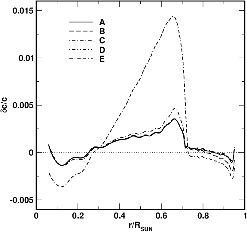
Refer to caption — Figure 1: Relative differences between the seismic sound speed derived by Basu et al. (2000) and the solar models presented in Table 2.

We have performed calibrations of the solar model with cesam2k with various sets of input physics and initial parameters. This consists in adjusting the initial parameters of the model (helium abundance and mixing-length parameter) in order to satisfy the observational constraints on the solar global parameters at solar age.

We have adopted the values of the astronomical and physical constants specified for the calculation of the stellar models compared in the different ESTA tasks (Lebreton et al., 2007, see). For the solar global parameters, we therefore took $R_{\odot}=6.9599\ 10^{10}\ {\rm cm}$ (radius), $L_{\odot}=3.846\ 10^{33}\ {\rm{erg.s^{-1}}}$ (luminosity) and $M_{\odot}=1.98919\ 10^{33}\ {\rm g}$ (mass). The value $R_{\odot}$ refers to the radius of the model layer where $T=T_{\rm eff}=5777$ K. For solar age, we adopted the value $t_{\odot}=4.57\ {\rm Gyr}$ (Bahcall & et al., 1995).

Table 2 presents the sets of input physics used in the different calibrations of solar models. All models have been calculated with the OPAL 2001 EOS (Rogers & Nayfonov, 2002) and the 1995 OPAL interior opacities (Iglesias & Rogers, 1996). Two sets of low temperature opacities have been used: the Alexander & Ferguson (1994) tables given for the Grevesse & Noels (1993) solar mixture and the Ferguson et al. (2005) tables given for the new solar mixture derived by Asplund et al. (2005) (see below). All models take into account the diffusion of chemicals due to pressure, temperature and concentration gradients (no radiative accelerations) but we considered either the Michaud & Proffitt (1993, hereafter MP93) or the Burgers (1969, hereafter B69) formalism. Convection is treated either according to the classical MLT (Böhm-Vitense, 1958, hereafter BV) or to the Canuto et al. (1996, hereafter CGM) formalism. In the CGM formalism, like in the CM formalism (Canuto & Mazzitelli, 1991), the contribution of eddies with different sizes is taken into account in the calculation of the convective flux and velocity. In addition Canuto et al. (1996) take into account the feedback of the turbulence on the energy input from the source which generates turbulent convection. For the atmosphere calculation we considered either the classical Eddington grey $T(\tau)$ -law or a law derived from Kurucz’s ATLAS 9 1-D model atmospheres (Kurucz, 1992). We have taken the same $T(\tau)$ -laws as used in the work by Samadi et al. (2006). These laws are based on model atmospheres calculated with either the BV or the CGM convection formulation. In both cases, the atmosphere calculation was performed adopting a value of the mixing-length parameter $\alpha_{\rm conv,atm}=0.5$ which allows to fit at best the observed profiles of the solar Balmer lines (van’t Veer-Menneret and Megessier, 1996, see). Therefore $\alpha_{\rm conv,atm}$ is different from the value of $\alpha_{\rm conv,int}$ in the interior, this latter being adjusted to calibrate the solar model. Finally, we adopted the GN93 solar mixture of heavy elements (Grevesse & Noels, 1993) in all models but one where we used the new AGS05 mixture (Asplund et al., 2005) which is derived from a time-dependent, 3-D hydrodynamical model of the solar atmosphere. The abundances of C, N, O of the AGS05 mixture are smaller than in the GN93 one which leads to an important decrease of the solar $(Z/X)$ ratio: $(Z/X)_{\odot}=0.0245$ for the GN93 mixture and $(Z/X)_{\odot}=0.0171$ for the AGS05 mixture.

Table 3 presents the results of the solar model calibrations. The relative differences in radius, luminosity and present $(Z/X)$ surface value of the five models A, B, C, D, E with the observed values are lower than $10^{-4}$ . The relative differences between the seismic sound speed derived by Basu et al. (2000) and the models are plotted in Fig. 1. The helioseismically measured values of the present radius at the base of the convective envelope $R_{\rm e,o}$ and of the present solar envelope helium abundance $Y_{e,o}$ provide strong constraints for the solar model. Basu & Antia (1997) helioseismically derived $R_{\rm e,o}=0.713\pm 0.001R_{\odot}$ . Boothroyd & Sackmann (2003) derived a mean value $Y_{\rm e,o}=0.245\pm 0.005$ from different helioseismic determinations. In all our models but one (model E), we find values of $Y_{e}$ and $R_{\rm e}$ in reasonable agreement with the seismic values. Model E is based on the AGS05 solar mixture which makes the agreement between the solar model and helioseismic observations much worse (Basu & Antia, 2004, see for instance). More details on the solar models calculated with cesam and their seismic properties can be found in Morel et al. (1999); Provost et al. (2000); Zaatri et al. (2007).

Acknowledgements.

We wish to express our thanks to A. Baglin and E. Schatzman for their suggestion to undertake the development of cesam and for their unfailing support. Many contributions to cesam, help, advice, debugging and constructive criticisms are from our nearest colleagues: G. Berthomieu, S. Brun, Th. Corbard, M.J. Goupil, A. Moya, B. Pichon, J. Provost, F. Thévenin, C. van’t Veer, J.P. Zahn. We acknowledge J. Christensen-Dalsgaard and M. Gabriel for private communications. Many stimulating and helpful discussions with: G. Alecian, N. Audard, A.I. Boothroyd, R. Cayrel, D. Cordier, W. Däppen, J.M. Marques, G. Michaud, J. Montalban, A. Noels, L. Piau, J. Reiter, S. Turck-Chièze, have brought many improvements. We express our gratitude to all of them. We wish to express our thanks to the anonymous referee whose comments and remarks greatly helped to improve the presentation of this paper.

References

Adelberger et al. (1998) Adelberger, E., et al.: Solar Fusion Rates. Rev. Mod. Phys. 70, 1265–1291 (1998)
Alécian & Michaud (2005) Alécian, G., Michaud, G.: About diffusivity, radiative viscosity and particles transport. A&A 431, 1–4 (2005)
Alexander & Ferguson (1994) Alexander, D. R. & Ferguson, J. W. 1994, ApJ, 437, 879
Anders & Grevesse (1989) Anders, E., Grevesse, N.: Abundances of the elements - Meteoritic and solar. Geochimica & Cosmochimica Acta 53, 197–214 (1989)
Angulo et al. (1999) Angulo, C., Arnould, M., Rayet, M., and the NACRE collaboration: A compilation of charged–particule induced thermonuclear reaction rates. Nuclear Physics A 656, 3–183 (1999)
Asplund et al. (2005) Asplund, M., Grevesse, N., & Sauval, A. J. 2005, in ASP Conf. Ser. 336: Cosmic Abundances as Records of Stellar Evolution and Nucleosynthesis, ed. T. G. Barnes, III & F. N. Bash, 25–+
Bahcall & et al. (1995) Bahcall, J. N., Pinsonneault, M.H., Wasserburg, G.J., Rev. Mod. Phys., 67, 781 (1995)
Basu & Antia (1997) Basu, S. & Antia, H. M., MNRAS, 287, 189 (1997)
Basu et al. (2000) Basu, S., Pinsonneault, M.H., Bahcall, J.H. ApJ, 529, 1084 (2000)
Basu & Antia (2004) Basu, S. & Antia, H. M. 2004, ApJ Let., 606, L85
Böhm-Vitense (1958) Böhm-Vitense, E.: Über die Wasserstoffkonvektionszone in Sternen verschiedener Effektivtemperaturen und Leuchtkräfte. Zs. f. Astrophys. 46, 108 (1958)
Boothroyd & Sackmann (2003) Boothroyd, A. I. & Sackmann, I.-J. 2003, ApJ, 583, 1004
Burgers (1969) Burgers, J.M.: Flow equations for composite gases. Academic Press, New york and London (1969)
Canuto et al. (1996) Canuto, V.M., Goldman, I., Mazzitelli, I.: Stellar turbulent convection - A Self-consistent Model. ApJ 473, 550– (1996)
Canuto & Mazzitelli (1991) Canuto, V.M., Mazzitelli, I.: Stellar turbulent convection - A new model and applications. ApJ 370, 295–311 (1991)
Caughlan & Fowler (1988) Caughlan, G.R., Fowler, W.A.: Thermonuclear Reaction Rates V. Atomic Data and Nuclear Data Tables 40, 284–334 (1988)
Chaboyer et al. (1999) Chaboyer, B., Demarque, P., Guenther D.B.: The Pulsation Properties of Procyon A. ApJ 525, L41–L44 (1999)
Clayton (1968) Clayton, D.D.: Principles of Stellar Evolution and Nucleosynthesis. Mc Graw–Hill, New York and London (1968)
Christensen-Dalsgaard (1988) Christensen-Dalsgaard, J.: Computational procedures for GONG solar model project, Astronomisk Institut, Aarhus Universitet (1988)
Christensen–Dalsgaard & Dappen (1992) Christensen–Dalsgaard, J., Dappen, W.: Solar oscillations and the equation of state. A&ARv 342, 267–361 (1992)
Cox (2000) Cox, A.N.: Allen’s Astrophysical Quantities. Springler/Verlag, Berlin (2000)
Cox & Giuli (1968) Cox, J.P., Giuli, R.T.: Principles of Stellar Structure, vol I & II. Gordon & Bretch, New-York, (1968)
Cox et al. (1989) Cox, A.N., Guzik, J.A., Kidman, R.B.: Oscillations of solar models with internal element diffusion. ApJ 342, 1187–1206, (1989)
De Boor (1978) De Boor, C.: A Practical Guide to Splines Springer, third ed., Berlin (1978)
Di Mauro (2004) Di Mauro, M.P.: Theoretical Aspects of Asteroseismology: Small Steps Towards a Golden Future. In: Danesy, D. (ed.) Helio and Asteroseismology, Toward a Golden Future, New Haven, Connecticut, 14–16 July, 186. Proceedings of the SOHO 14 / GONG 2004 Workshop (ESA SP-559) New Haven, Connecticut (2004)
Eggenberger et al. (2005) Eggenberger, P., Carrier, F., Bouchy, F.: Models of Procyon A including seismic constraints. New Astronomy 10, 195–208 (2005)
Eggleton (1971) Eggleton, P.: The evolution of low mass stars, MNRAS 151, 351 (1971)
Eggleton et al. (1973) Eggleton, P.P., Faulkner, J., Flannery, B.P.: An Approximate Equation of State for Stellar Material, A&A 23, 325 (1973)
Ferguson et al. (2005) Ferguson, J. W., Alexander, D. R., Allard, F., et al. 2005, ApJ, 623, 585
Gabriel (1997) Gabriel M.: Influence of heavy element and rotationally induced diffusions on the solar models. A&A 327, 771–778 (1997)
Grevesse & Noels (1993) Grevesse, N., Noels, A.: Cosmic Abundances of the Elements. In: Prantzos, E. Langioni-flam, M. Casse (eds.) Origin and Evolution of the Elements. Cambridge Univ. Press, 14, (1993)
Grevesse & Sauval (1998) Grevesse, N., Sauval, A.J.: Standard Solar Composition. Space Science Revue, 85, 161-174 (1998)
Henyey et al. (1965) Henyey, L.G., Vardya, M.S., Bodenheimer, P.L.: Studies in Stellar Evolution. III. The Calculation of Model Envelopes. ApJ 142, 841 (1965)
Hairer & Wanner (1991) Hairer, E., Wanner, G.: Solving Ordinary Differential Equations II, Springer-Verlag, Berlin (1991)
Iben (1965) Iben, I.: Stellar evolution I. The approach to the mazin sequence. ApJ 141, 993–1018 (1965)
Iben & MacDonald (1985) Iben, I., MacDonald, J.: The effect of diffusion due to gravity and due to composition gradients on the rate of oxygen burning in a cooling degenerate dwarf. ApJ 296, 540–553 (1985)
Iglesias & Rogers (1996) Iglesias, C. A. & Rogers, F. J. 1996, ApJ, 464, 943
Kippenhahn & Weigert (1991) Kippenhahn, R., Weigert, A.: Stellar Structure and Evolution, Springer-Verlag Berlin (1991)
Kurucz (1992) Kurucz, R.L., Rev. Mex. Astron. Astrofis. 23, 45 (1992)
Lebreton et al. (2007) Lebreton, Y. Monteiro, M.J.P.F.G., Montalbán, J., Baglin, A., Michel, E. 2007, in Astrophys. Space Sci. (CoRoT/ESTA Volume), Springer
Lide et al. (1994) Lide, D.R., et al.: CRC Handbook of chemistry and physics 75th edition 1994 CRC press Boka Raton : Ann Arbor : London : Tokyo (1994)
Mathis & Zahn (2004) Mathis, S., Zahn, J.P.: Transport and mixing in the radiation zones of rotating stars. I. Hydrodynamical processes, A&A 425, 229–242 (2004)
Mathis et al. (2004) Mathis, S., Palacios, A., Zahn, J.P.: On shear-induced turbulence in rotating stars, A&A 425, 243–247 (2004)
Michaud & Proffitt (1993) Michaud, G., Proffitt, C.R.: Particle transport processes. In: Baglin & W.W. Weiss (eds.) Inside the Stars, San Francisco: ASP conf. ser. 40, 246–249 (1993)
Mihalas (1978) Mihalas, D.: Stellar Atmosphere. Freeman and Cie, New York (1978)
Mihalas & Weibel-Mihalas (1984) Mihalas D., Weibel-Mihalas B.: Foundations of Radiation Hydrodynamics, Oxford University Press, Oxford (1984)
Mihalas et al. (1988) Mihalas D., Dappen, W., Hummer, D.G.: The equation of state for stellar envelopes. II - Algorithm and selected results. ApJ 331, 815–825 (1988)
Mitler (1997) Mitler, H.E.: Thermonuclear ion-electron screening at all densities. I - Static solution. ApJ 212, 513–532 (1997)
Morel et al. (1994) Morel, P., van’t Veer, C., Provost, J. Berthomieu, G., Castelli, F., Cayrel, R., Lebreton, Y.: Incorporating the atmosphere in stellar structure models: the solar case. A&A 286, 91–102 (1994)
Morel (1997) Morel, P.: CESAM a code for stellar evolution calculations. A&AS 124, 597–614 (1997)
Morel & Thévenin (2002) Morel, P., Thévenin, F.: Atomic diffusion in stellar models of type earlier than G. A&A 390, 611–620 (2002)
Morel et al. (1999) Morel, P. and Pichon, B. and Provost, J. and Berthomieu, G.: Solar models and NACRE thermonuclear reaction rates. A&A 350, 275 (1999)
Palacios et al. (2003) Palacios, A., Talon, S., Charbonnel, C., Forestini, M.: Rotational mixing in low mass stars : I Effects of the $\mu$ gradient in main sequence and sub-giant Pop I stars. A&A 399 603–617 (2003)
Paquette et al. (1986) Paquette, C., Pelletier, C., Fontaine, G., Michaud, G.: Diffusion coefficients for stellar plasmas. ApJS 61, 177–195 (1986)
Press et al. (1986) Press, W.H., Flannery, B.P., Teukolsky, S.A., Vetterling, W.T.: Numerical Receipes, Cambridge University Press, Cambridge (1986)
Proffit & Michaud (1991) Proffit, C.R., Michaud, G.: Diffusion and mixing of lithium and helium in population II dwarfs. ApJ 371, 584–601 (1991)
Provost et al. (2000) Provost, J. and Berthomieu, G. and Morel, P.: Low frequency p- and g- mode solar oscillations. A&A 353, 775 (2000)
Quarteroni & Valli (1994) Quarteroni A., Valli A.: Numerical approximation of partial differential equations, Springer-Verlag, Berlin (1994)
Rogers & Nayfonov (2002) Rogers, F. J. & Nayfonov, A. 2002, ApJ, 576, 1064
Salpeter (1961) Salpeter, E.E.: Energy and Pressure of a Zero-Temperature Plasma. ApJ 134, 669 (1961)
Samadi et al. (2006) Samadi, R. and Kupka, F. and Goupil, M. J. and Lebreton, Y. and van’t Veer-Menneret, C.: Influence of local treatments of convection upon solar p mode excitation rates A&A 445, 233–242 (2006)
Schumaker (1981) Schumaker, L.: Splines Functions: Basic Theory. John Whiley, New-York (1981)
Stoer & Bulirsch (1979) Stoer, J., Bulirsch, R.: Introduction to Numerical Analysis. Springer-Verlag, Berlin (1979)
Talon et al. (1997) Talon, S., Zahn, J.P., Maeder, A., Meynet, G.: Rotational mixing in early-type stars: The main-sequence evolution of a 9Msun star. A&A 322, 209–217 (1997)
Thomas (1930) Thomas, L.H.: The Radiation Field in a Fluid in Motion. Quart. J. of Math. 1, 239 (1930)
Thoul et al. (1994) Thoul, A.A., Bahcall, J.N., Loeb, A.: Element diffusion in the solar interior. ApJ 421, 828–842 (1994)
Turcotte et al. (1998) Turcotte, S., Richer, J., Michaud, G.: Consistent Evolution of F Stars: Diffusion, Radiative Accelerations, and Abundance Anomalies. ApJ 504, 559 (1998)
van’t Veer-Menneret and Megessier (1996) van’t Veer-Menneret, C., Megessier, C.: Effective temperature of A and F stars from Balmer line profiles, and the Infrared Flux Method. A&A 309, 879 (1996)
Zaatri et al. (2007) Zaatri, A. and Provost, J. and Berthomieu, G. and Morel, P. and Corbard, T.: Sensitivity of the low degree solar oscillations to the change of solar abundances A&A 269, 1145 (2007)