Abstract
In production processes, e.g. or , the and overlap in the same partial wave. The conjecture of Extended Unitarity (EU) states that the pair should have the same phase variation as elastic scattering. This is an extension of Watson’s theorem beyond its original derivation, which stated only that the -dependence of a single resonance should be universal. The prediction of EU is that the deep dip observed in elastic scattering close to 1 GeV should also appear in production data. Four sets of data disagree with this prediction. All require different relative magnitudes of and . That being so, a fresh conjecture is to rewrite the 2-body unitarity relation for production in terms of observed magnitudes. This leads to a prediction different to EU. Central production data from the AFS experiment fit naturally to this hypothesis.
PACS numbers: 13.25.-k, 13.25.Gv, 13.75.Lb
Experimental disagreements with Extended Unitarity
D. V. Bugg11 1 email: D.Bugg@rl.ac.uk
Queen Mary, University of London, London E1 4NS, UK
1 Introduction
In its simplest form, the idea of Extended Unitarity (EU) states that the pair in a single partial wave should have the same phase variation with in all reactions as in elastic scattering. This idea originates from Aitchison [1] and has been adopted in various guises by many authors. His arguments will be presented in detail in Section 2, so as to expose the assumptions and consequences. At the time the idea was introduced, it was a reasonable conjecture; now modern data allow it to be checked accurately, but disagree with it.
Many experimental groups have made extensive fits to production data using a -matrix approach based on EU. These fits are excellent; no criticism is intended of their quality. Experimentalists have found empirically the necessary freedom to get good fits to data. However, on close inspection, this freedom is inconsistent with strict EU.
This whole topic has been the subject of extensive discussion with many authors. There is a bewildering jungle of claims and counter-claims. My objective is to cut a path through this tangle and expose where problems lie; this makes the presentation pedantic in places.
Aitchison’s essential point is that all processes should be described by a universal denominator , where is the same as for elastic scattering; is Lorentz invariant phase space. The assumption which is being made is that Watson’s theorem [2] applies to the coherent sum of all components in the partial wave. This is a step beyond Watson’s derivation, which referred only to a single eigenstate; Watson did not consider overlapping resonances.

In elastic scattering, the is superimposed on a slowly rising amplitude associated with the pole. Cern-Munich data [3] show that the phases of these two components add. Below the threshold, both and -matrices are confined to the unitarity circle if we neglect the tiny inelasticity due to . Unitarity may be satisfied by multiplying -matrices of and , as suggested by Dalitz and Tuan [4]. This fits the data within errors of .
Fig. 1 shows the Argand diagram for the S-wave from my recent re-analysis of these (and other) data [5]. From BES data on , the has a full-width at half-maximum of MeV [6]. The combined phase shift rises rapidly from at 0.88 GeV to near 1.1 GeV. There is a deep dip in the cross section where the combined phase goes rapidly through . The crucial point of EU is that this feature should be common to production processes.

BES data on [6] immediately require a modification of the rudimentary form of EU. The mass spectrum in these data is reproduced in Fig. 2. There is a dominant contribution and a small interfering contribution; this is very different to elastic scattering. Lähde and Meissner [7] modify the conjecture of EU to apply separately to strange and non-strange components, i.e. to the scalar form factors for and .
The dip in the elastic cross section at 989 MeV is a very delicate feature. If, for any reason, relative magnitudes of and change, the zero at 989 MeV can disappear quickly; here and elsewhere, will denote unless there is confusion with other ’s. If the phase of changes with respect to the , the mass at which the dip appears will likewise change. The interference region between and is an ideal place to check Extended Unitarity.
Two considerations will play a critical role: unitarity and analyticity. Unitarity is often quoted and plays an essential role in setting up the current -matrix formalism which treats both elastic scattering and production on the same basis. For a production reaction, Aitchison conjectures a unitarity relation for the production amplitude :
| (1) |
He defines his to be proportional to , where refers to production:
| (2) |
Dividing both sides of (1) by ,
| (3) |
It is odd that on the right-hand side is multiplied by , unless . However, experiment will require different contributions to from and .
Consider next analyticity. Dispersion relations connect magnitudes and phases. If the relative magnitudes of and change from those of elastic scattering because of matrix elements, their relative phases must also change. Conversely, analyticity predicts that if the phase variation with of the amplitude is universal, as EU demands, so is the variation with of the magnitude (up to a constant scaling factor); for the simplest situation where only resonances are present, the relative magnitudes of , and any further must be almost the same in production as elastic scattering. This is a point which has almost always been ignored.
The word ‘almost’ represents a caveat: there may in addition be a polynomial is which can be different between elastic scattering and production. It turns out that one can plausibly limit deviations of relative magnitudes within . This question is discussed in subsection 2.1. Experiment requires larger deviations than this in the four sets of data discussed here. This implies phases must change from those predicted by EU. Experimentalists have correctly allowed for this by using complex coupling constants in the isobar model.
Section 3 compares the prediction of EU with 3 sets of data. The first concerns BES data for [8]. The non-strange components of and dominate both elastic scattering and . From Aitchison’s algebra and that of Lähde and Meissner, it follows that the amplitude should have almost the same magnitude as the amplitude, as well as the same phase as elastic scattering. This prediction is contradicted by the data, where no is visible and a fit to the data places a low limit on it.
The next two sets are Crystal Barrel data for , where and are clearly visible [9]. One set is for annihilation in liquid hydrogen and the other for gaseous hydrogen. Annihilation from the initial state is 13% in liquid and 48% in gas, allowing a clear separation of amplitudes for production of and from and . Results for both are inconsistent with the deep dip of elastic scattering predicted by EU.
Section 4 concerns data from the AFS experiment on central production: [10]. Here one expects the protons in the final state to act as spectators. However, EU still fails conspicuously to fit the data. This important result leads to a revised form of the unitarity relation, as follows.

Fig. 3 sketches the usual diagrammatic approach to the unitarity relation. It may be derived by cutting the diagram down the middle, along the dashed line. For a 2-body system of , , , etc. the resulting relation is well known:
| (4) |
The application of 2-body unitarity assumes that the pions interact only with one another, not with any spectator. In most sets of data there are large signals where pions do interact with the spectator. For , as an example, the channel accounts for 40% of events [8]. Some of it may be generated by pions from decays of or rescattering from the spectator; this is a so-called triangle graph. Aitchison himself remarks that this can distort the unitarity relation. This provides one reason why EU may fail for the first three sets of data; it does not explain the fourth, where some further effect is required.
There are fundamental differences between elastic scattering and production. In , for example, matrix elements and dictate the magnitudes of these amplitudes; any values are possible. This differs from elastic scattering, where and magnitudes are fixed purely by their coupling constants to . Equation (3) is an asymmetric relation, allowing and to be produced with different magnitudes, but requiring that they rescatter an in elastic scattering. A more logical alternative is the symmetric relation
| (5) |
hence . This relation fits AFS data for central production naturally, whereas EU does not. If the is absent from production data, (5) reduces to the obvious relation ; Aitchison’s form of the relation, taken with analyticity does not allow the to be absent, as we shall see in Section 2.
Section 5 suggests a new way of fitting 2-body data. Section 6 then summarises conclusions.
2 The hypothesis of Extended Unitarity
In a two-body process, the scattering of a pair of pions to final states , , , and must satisfy unitarity. The -matrix for these coupled channels may be written in terms of a real -matrix as
| (6) |
It is normalised here so that . Below the inelastic threshold
| (7) |
The -matrices used here will include couplings to all channels. However, it simplifies the presentation of essential points to reduce the formalism initially to a single channel. This simplication is sufficient to expose the basic issues, and can be generalised later to include inelasticity.
The approach of Aitchison [1] will now be outlined. I am grateful to him for clarifying the algebra in more detail than is to be found in the original publication. Suppose -matrices multiply, i.e. phases add. Let and be -matrices for and respectively. The elementary expression for then gives a -matrix for elastic scattering
| (8) |
from which it follows that the -matrix for elastic scattering is
| (9) |
Aitchison now conjectures that an amplitude for producing a two-body channel present in may be written in terms of a vector , with
| (10) | |||||
| (11) |
where and are constants for production couplings. With this ansatz, the relation
| (12) |
known as Extended Unitarity, is automatically satisfied. It is a consequence of (10) that has the same phase as . Substituting (8) and (11) in (10) gives, in this one-channel case
| (13) | |||||
| (14) |
where . From (13), the phase of is indeed , as imposed by (10). Equation (14) will play the decisive role in comparisons with experiment.
In (14), and . At 989 MeV, and . So both terms are very close to zero, regardless of the values of and . This predicts that production data should have the same deep dip at this energy as elastic scattering.
There is a further point. In the second term, over a sizable mass range. In the first term, should be conspicuous, since it has a rapid phase variation and the same peak magnitude as , which is itself clearly visible in all sets of data considered here. However, the data all require the magnitude of the to be smaller than predicted.
The key point is that the factor of (13) leads directly to the factor in the first term of (14). The first and third sets of data will require of (14) to be small. In the elastic region, the first term becomes
The bizarre conclusion of EU is that the phase of the is present even though . This is inconsistent with analyticity. It will be shown in Section 3 that experiment disagrees with EU even without the constraint of analyticity. However this additional constraint makes conclusions more definitive.
2.1 Analyticity
For purely elastic scattering, the Omnès relation [11] reads [including a factor in ]:
| (15) | |||||
| (16) |
where P denotes the Principal Value integral. We shall not actually need to evaluate (16). It plays only a conceptual role and this needs considerable explanation. The basic point is that contains both real and imaginary parts, so determines both. For elastic scattering is real. It arises from the left-hand cut, i.e. meson exchanges between the two pions.
With inelasticity, corresponding relations may be written in a 2-channel form. Then is replaced by , the angle makes to the real axis when measured from the origin of the Argand diagram, see Fig. 12 of subsection 4.1.
If EU is valid, the production amplitude may be written . In principle could be anything, depending on production dynamics. However, we have quite precise experimental information about it. An extreme view is that and of (13) can be arbitrary and complex. However if they are complex this leads directly to a conflict with EU. Equation (14) contains two parts and . Substituting Breit-Wigner formulae for and , the first term becomes . This is real but has a specific -dependence in the numerator as well as in the denominator. If or becomes complex, the numerator becomes complex. This then introduces a phase variation separate from . The “prediction” of EU is distorted by this extra phase. Only if is real does EU survive in its strict form.
Many experimental groups have used the P-vector approach using complex coupling coefficients, without realising that this destroys the universality of the phase variation with . This is what experiment demands, so they have done the right thing. But the use of the universal denominator is no longer logically correct. One might as well fit directly in terms of complex coupling constants and individual -matrices for each resonance.
2.2 Form Factors
There is a further fundamental point. For elastic scattering, is uniquely related to by both unitarity and analyticity. At first sight it appears that analyticity relates in the same way to in production reactions, with the result , where is a constant. This requires : if the phase of the amplitude is universal, relative magnitudes of and must also be universal.
There is however a caveat. A more fundamental form of the unitarity relation (12) is that the discontinuity of across the elastic branch cut is . Then may be multiplied by a polynomial , providing it does not have a discontinuity along the real -axis. A few examples will hopefully clarify ideas. Firstly, a form factor in is one such example, arising from the sizes of particles, i.e. from matrix elements. Secondly, in , the E1 transition has an intensity proportional to the cube of the photon momentum; this inflates the lower side of the . Thirdly, in , there is an centrifugal barrier for the production process. Fourthly, in some special cases, matrix elements may go through zero as a function of . Taking to be real, let us write in general
| (17) |
A feature of all production data considered here is a strong low-mass peak due to the pole. This peak is not present in elastic scattering because of an Adler zero in the elastic scattering amplitude at , just below the threshold. The elastic amplitude rises approximately linearly with and there is no low mass peak. The origin of the difference has been known to theorists for at least 20 years. Au, Morgan and Pennington [12] pointed out that the difference between elastic scattering and central production data can be accomodated by using the same Breit-Wigner denominator for both, but replacing the numerator by something close to a constant. This polynomial is allowed because is outside the physical region. Data require , hence . More exactly,
| (18) |
for the parametrisation of the amplitude in [13]. In practice, quadatic and cubic terms in are very small and under tight control from fits to data up to 1.8 GeV.
For , the pole is visible by eye in Fig. 4(a) below. The phase of the amplitude in this reaction is experimentally the same as in elastic scattering within [14]. Values of can be determined directly from the data. The same is true of the [15], which likewise has an Adler zero in the numerator for elastic scattering, but not for production. In both cases, is consistent within errors with a constant; the Adler zero in the numerator of elastic scattering has disappeared. One can try fitting the and poles in production data with the conventional form factor , where is momentum in the production channel. For both, optimises at slightly negative values, which are unphysical. For the , fm2 with confidence and for the , fm2 at the same level.
A crucial piece of information in testing EU will be relative magnitudes of and . The magnitude of the amplitude is easily separated from the tail of the at 920 MeV, three half-widths from 989 MeV. If is determined at this energy and at 400 MeV, the amplitude changes by at 989 MeV for the confidence level quoted above. However, this exaggerates the error, since there are compensating changes in the line-shape fitted to the amplitude. Realistically, changes are half this. Adding in quadrature uncertainties in the line-shape due to the opening of the threshold, the uncertainty in the amplitude extrapolated from 920 to 989 MeV is with confidence. This provides a tight constraint on the relative magnitudes of and amplitudes if EU is correct. This disposes of the paradox that the phase of can be present with .
From this point onwards, it will be assumed that EU should be supplemented with the condition imposed by analyticity within .
2.3 Formulae for and
Formulae and numerical parameters for the amplitude are to be found in Refs. [13] and [5]. The coupling has been fitted to four sources: (i) phase shifts deduced from Cern-Munich data by Ochs [16], (ii) data of Pislak et al. [17], (iii) predictions of phase shifts by Caprini et al. [18] using the Roy equations, and (iv) BES data on [8].
The coupling to and has been fitted to available data on those channels [19], and in [5] the coupling has been derived from Cern-Munich data. There is close consistency between all these sets of data. Because Refs. [13] and [5] fit the same data with different formulae, the amplitudes agree within errors up to 1.2 GeV. Those of Ref. [5] are more cumbersome to use, since they allow for the dispersive effect of the threshold. Therefore the first and fourth sets of data discussed below are fitted with the formulae from Ref. [13].
The general procedure adopted here is to allow the parameters of the to have the freedom allowed in earlier determinations of its parameters, but no extra freedom in the vicinity of . In testing EU, the magnitude of is restricted to the discussed above; its phase is allowed the freedom with which its parameters are known.
2.4 Parameters of
The is so narrow that it is readily separated from the . The BES data on shown in Fig. 2 exhibit a very clear signal. An important point is the excellent mass resolution and mass calibration of the BES detector, MeV. Both are easily checked for the channel against the very precisely known parameters of . Data from the same publication [6] on contain a clear peak, and the two sets of data determine accurately the ratio of couplings to and . An important detail is an error in units in [6]: is reported as 165 MeV; this should read 0.165 GeV2.
The Breit-Wigner denominator for the amplitude is and has to be continued analytically below the threshold as . Without direct information on the channel, this term gets confused with [20]. Any form factor applied to adds to the confusion. One only has to glance at the Particle Data Tables [21] to see the large spread in parameters fitted to the (and ) in experiments having no direct information on the branching ratio between and . Unfortunately, the PDG does not report the BES determination of , which is the best in the published literature because of the availability of a clear signal in .
It was shown in [19] that the BES parameters for are closely consistent with Kloe data [22] on when one allows for interference between and . This paper determines . BES data on confirm a large value for this ratio [23]. The full width at half-maximum (34 MeV) agrees well with Cern-Munich data MeV [3]. It also agrees closely with the full-width of the signal in Crystal Barrel data MeV). The BES parametrisation will therefore be adopted in fitting the AFS data. Further checks from Belle, Babar and Cleo C will be very welcome.
3 Experimental tests
3.1
Considerable detail needs to be given of fits to experimental data, in order to pin down the disagreements with EU. The prime conclusions which will emerge are that (i) the amplitude does not follow that of elastic scattering, (ii) the magnitude of the amplitude, relative to , is much smaller than predicted by Eq. (14), regardless of analyticity which also requires that their relative magnitudes should be the same within .

Fig. 4 displays features of BES data for [8]. There is a clear peak in Fig. 4(a) at GeV due to the pole. Its shape is cleanly separated from the contribution up to 1.05 GeV, where the rapidly overtakes it. The data include a slowly varying background which is included in the fit. There is also a well defined slowly varying component due to the reflection of . Both are shown in the experimental publication.
There are two amplitudes for production of and , with orbital angular momenta and in the production reaction. The amplitude includes a centrifugal barrier for production which optimises at a radius of 0.8 fm (roughly as expected for convolution of wave functions of , and ). For the isobar model fit, different magnitudes are allowed for and 2, with complex coupling constants, though it turns out that the contribution from is negligible. In the EU fit the relative phases of and components are constrained to be the same, and relative magnitudes are constrained to be the same within . In Figs. 4(a) and (c), the lower histogram shows the intensity: from the isobar model fit in (a) and from EU in (c). The upper histogram, close to data points, shows the result of the full fit. Unfortunately, the mass projection alone is not definitive, for reasons explained shortly. One low point in the mass projection just above 1 GeV hints at a dip following the EU prediction.
However, there is a great deal more information contained in the Dalitz plot of Fig. 4(b) and also in the correlation between the decay plane and the production plane. In the Dalitz plot, there are strong horizontal and vertical bands due to . These bands interfere with and (and if present). Note that the decays mostly through -waves, so its intensity would be almost constant across the Dalitz plot in the absence of interferences. Also note from the lower histogram of Fig. 4(a) that the amplitude at 950 MeV is sizable. Cross-hairs on Fig. 4(b) show where a pair of mass 1 GeV intersects the band. If were present with the same magnitude as and with the phase predicted by EU, a large but narrow interference with cannot be avoided due to , whatever the relative phase of . It should have a full width of GeV2 along the band: the line-width of . There should also be a dip somewhere along the diagonal at GeV. Fig. 4(d) shows an enlarged view of this region. There is no sign of these features.
The decay plays an important role. The spin of the lies along the normal to its decay plane; information on this decay plane is a key ingredient in determining helicity amplitudes. These are essential to determine interferences between the amplitudes for , and . There are in principle five amplitudes corresponding to production with (one amplitude), (three) and (one). It turns out that the amplitude and one of the three amplitudes are negligible. There are large interferences between and the remaining three amplitudes and even larger interferences with .
With the EU hypothesis, the best fit to the Dalitz plot (upper histogram) and the decay plane fills in the predicted dip at GeV2 with other interferences, see Fig. 4(c); however, the price is a considerable deterioration of log likelihood compared with the fit of Fig. 4(a). The isobar model fit is better than EU by 259 in log likelihood. There are two reasons. Firstly, the narrow does not appear in interferences with either or . The mass resolution of the BES data is 4 MeV in at 950 MeV; searching for the with accurately known line-shape is limited purely by statistics and there are K events. Secondly, in the fit based on EU, there are strong conflicts between interference terms amongst , and . The data want slowly varying interferences between and the broad , instead of rapidly varying interferences of the narrow with and/or .
There are two extra fitting parameters for the isobar model fit: i.e. two complex coupling constant for instead of one. [The amplitude is negligible]. The definition of log likelihood is such that a change of 0.5 corresponds to a one standard deviation change in one variable. For large statistics, is approximately twice the change in log likelihood. So the fit of Fig. 4(a) is better than EU by 19.7 standard deviations statistically.
It is important to remark that the BES publication gives a second fit done independently. This shows a mass projection almost identical with the scalar form factor. This requires a very strong , in conflict with what one can see by eye in Fig. 4(d). However, this analysis made no use of the decay plane. Without that information, it is impossible to disentangle the magnitudes of the five amplitudes; the determination of the magnitude and phase of the signal becomes very poor. I have rechecked the analysis omitting information from the decay plane. No stable fit emerges with the mass projection of the second fit in the BES publication, and there is no evidence for the presence of at all in this fit. The only explanation I can find of this second BES fit is that the relative magnitudes of and have been constrained to agree with the scalar form factor. This is, of course, exactly what needs to be checked in the present work.

.
Fig. 5 shows the Argand diagram for from my fit to and ; the factor is included so that the diagram goes to zero at the threshold. The ratio of and amplitudes is at 0.99 GeV and the lags the by . At the top of a large loop due to the , there is a small structure due to . For comparison purposes, the dashed curve shows the amplitude alone and the dotted curve shows the EU prediction normalised to the full curve at 0.47 GeV, the peak of the . The essential point is that the deep dip in this latter curve near the mass is missing from the data. There is one qualitative feature of Fig. 5 which will be important later. The amplitudes in a production process are free to add vectorially in any way required by the data. This situation is quite different from elastic scattering, where the amplitude is constrained to the unitary circle.
It is now necessary to consider a number of systematic questions which might blur the argument against EU. Corresponding remarks will apply to fits to the other three sets of data.
Firstly, could the disappearance of the predicted arise from effects of the threshold? The answer is no, because the appears clearly in elastic scattering and the prediction of EU is that it should be almost identical in production. A precise cancellation of the magnitude and phase of the predicted would be needed. This is ruled out by the known couplings of both and to . The analytic continuation for the below the threshold is accurately determined over the small mass range concerned by BES data on and . In the amplitude, the inelasticity rises over a mass scale of 200 MeV as shown in Fig. 11 of Ref. [19]. Any flexibility in the analytic continuation of the term then has a scale of MeV. Furthermore, it is closely constrained by the fit to Kloe data on . So this explanation is highly implausible.
Secondly, could the BES data be fitted assuming , followed by ? This has been tested by adding fitted freely. Its magnitude optimises at zero within errors. It improves log likelihood only by 2.
3.2 An objection of Aitchison
Thirdly, Aitchison argues [24] that a further term might be added to the -vector due to dynamics of the production process. A similar approach was used in fits by Bowler et al. and Basdevant and Berger to the to allow for the Deck effect [25] [26] [27]. An additional term appears in . If , the second term can cancel the term of EU, leaving and the first of the additional terms, which is close to 0 since . This removes almost all the structure due to . However, this cancellation also leaves a term and when is small this becomes , which is much larger than the term itself if is a constant. This is ruled out by the data, so it becomes necessary to tailor the -dependence of to reproduce the magnitude of the amplitude.
However, this is not the end of the story. Phase information is also available. In [14] it is shown that interference between and measures the phase of the amplitude (plus any background term ) and requires it to be the same as for elastic scattering down to 450 MeV with an error of in the worst scenario, see Fig. 2 of that paper. It is worth mentioning that there is a similar result for the in [15]. Fig. 4(a) of that paper shows that the phase from BES data on agrees with the LASS effective range formula for elastic scattering down to 750 MeV within . Fig. 4(f) of the same paper shows a corresponding agreement for E791 data on within a similar error. These results rule out any background different from and with a magnitude larger than and a phase difference above . They of course agree with Watson’s original statement that of a single resonance should be universal.
There is no obvious source of the background proposed by Aitchison, as there was in [25], where a Deck background was visible in the data and made a contribution to cancelling the amplitude. A similar fortuitous cancellation with unidentified backgrounds will be required also for all three of the following sets of data. In all cases, the additional background gives rise to a phase variation different to strict EU. If the background removes the , only the is left, i.e. , which contributes only part of the phase of elastic scattering; so the amplitude does not satisfy EU.

3.3
A fresh analysis of Crystal Barrel data on annihilation at rest to has been completed recently [5]. Data are available with statistics of K events (and experimental backgrounds) in both liquid and gaseous hydrogen; these allow a good separation of and initial states. Although the appears clearly in annihilation, the magnitude of the S-wave amplitude does not go to zero on the Argand diagram near 1 GeV, as EU predicts. This Argand diagram is reproduced in Fig. 6(a). Its magnitude is smallest at 0.98 GeV, but is still very distinct from zero. For annihilation, the fitted amplitude, relative to , is much smaller, see Fig. 6(b). The magnitude of the amplitude is quite large near 1 GeV.

The question arises how robust these solutions are. Could they ‘bend’ to accomodate EU? The published analysis requires some -dependence of the numerator fitted to the amplitudes, of the form , with complex . Can extra flexibility reach agreement with EU? A second point is that the analysis does not include the repulsive S-wave. Could this bring conclusions into line with EU?
The brief answer is definitely no, and will be presented graphically. Fig. 7(a) shows the mass projection for data in liquid from the current analysis; it fits the data points accurately. In Fig. 7(b), the combination of the isobar model is replaced by the EU combination (with the constraint from analyticity that magnitudes of and should be equal within ). Initially, only the coupling constant of this combination is refitted, leaving other amplitudes untouched; this is for the purpose of illustrating the change required by EU. The component is large and cannot change much; a deep dip appears at 1 GeV because of the corresponding dip in the elastic amplitude.
It is of course necessary to re-optimise all components. The resulting mass projection is shown in Fig. 7(c) and is still in severe disagreement with the data. A measure of the disagreement may be obtained from . Here, it is necessary to point out that even the fit of Fig. 7(a) has a larger than 1. This is probably because of the enormous statistics and small, slowly varying systematic errors in acceptance. The procedure adopted here is to renormalise to 1 per point for this fit and apply the same scaling factor to all other fits. The fit of Fig. 7(c) then has a renormalised of 40599 for 3500 bins; this is a 170 standard deviation discrepancy, allowing for the reduction in the number of fitted parameters by 2.
A much better fit is possible if relative magnitudes of and are allowed to vary. The phase of the S-wave amplitude in Fig. 6(a) is close to EU, and only a 10 MeV shift is required for a perfect fit. This is consistent with the energy calibration and resolution of the Crystal Barrel detector. However, the fitted combination of amplitudes no longer agrees with the crucial equation (14).
Fig. 7(f) shows the effect of including the S-wave amplitude, using the formulae of Section 4.1 of Ref. [5]. There is only a rather small improvement, because the slow -dependence of this amplitude cannot fill the narrow dip at 1 GeV. The renormalised falls to 34345, a discrepancy of .
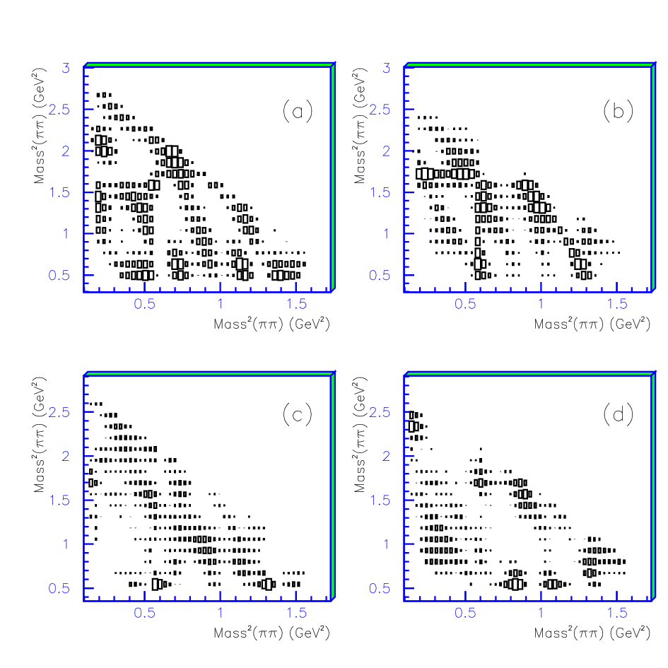
It is not just the mass projection which governs . One should inspect discrepancies in all over the Dalitz plot. Fig. 8 makes such a comparison. Panel (a) shows discrepancies in where the fit is above the liquid data and (b) the discrepancies where the fit is low. Panels (c) and (d) show results for data in gas. One sees striking systematic discrepancies all over the Dalitz plot, arising from interferences. Such discrepancies are almost completely absent from the fit of Fig. 7(a) using the isobar model.
There are two further points for discussion. In the work shown on Figs. 7(e) and (f), the S-wave was fitted without factoring out the Adler zero which occurs at . If this is done (as for the amplitude), the broad amplitude gets confused with the amplitude and leads to minor improvements all over the Dalitz plot. However, none of these is distinctive enough to require the amplitude definitively.
Secondly, could a more complicated polynomial than multiply the amplitude and give a successful fit? Extensive tests were made in [5] with the objective of improving the fits reported there. If one chooses too free a polynomial, the fitted component in gaseous hydrogen can fluctuate wildly from the 50% predicted from Stark mixing by Reifenrofer and Klempt [28]. To avoid this, the fitted component is constrained within the range . Unless the numerator of the EU amplitude is designed to include a narrow dip at 1 GeV, no large improvement is observed.
One further observation from the Crystal Barrel data is worth reporting. Relative intensities of and are quite different in annihilation to those in elastic scattering. In data, the integrated intensities of these two resonances are equal within after allowing for the (modest) effects of centrifugal barriers for production ( for annihilation and for ). However, in elastic scattering the fitted width is a factor 4 smaller than that of . This again disagrees with EU.
4 Central production of
Central production of a pair in was fitted using EU by Au, Morgan and Pennington (AMP) [12]. In data from the AFS experiment at the ISR [10], the two final-state protons are produced with very small 4-momentum transfers GeV2. It is routinely assumed that the pair is unaffected by final state interactions with these protons, which are separated from the central region by a gap in rapidity.
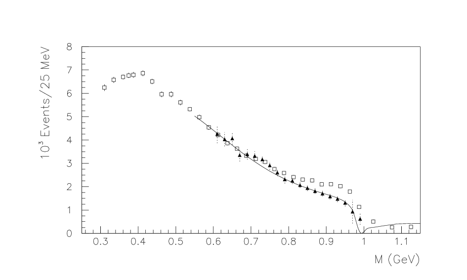
AMP draw attention to structure in the mass spectum similar to the dip in the S-wave elastic cross section. Fig. 9 shows the AFS data as open squares. There is a peak at low mass, close to that of the pole in BES data, but not quite identical, for reasons discussed shortly.
Triangles on Fig. 9 show elastic cross sections derived from Cern-Munich phase shifts; this is done by dividing the amplitude of elastic scattering by , leaving only the term . The curve shows my fit to elastic data after dividing the amplitude by . The agreement between the curve and triangles demonstrates that the parametrisation of the reproduces Cern-Munich phase shifts. Results are similar to the AFS data, but there is a distinct difference in the vicinity of . What is clearly evident is constructive interference between and immediately below 989 MeV, where EU predicts a zero. Even without fitting, one can see that EU will fail.
A detail is that, up to the threshold, one piece of information from each Cern-Munich moment is sufficient to determine phase shifts for both S- and P-waves. Above the threshold, however, the separation of inelasticity parameters and phase shifts cannot be made without further assumptions. Just above the threshold, the solution of Ochs [16] has 0.6-0.7, whereas the BES line-shape for demands parameters dropping to at 1.01 GeV. In view of this large discrepancy, predictions from Cern-Munich phase shifts are not shown above the threshold.

Since the work of Morgan and Pennington [29], information on both and has improved enormously. The amplitude is taken (within errors) from Ref. [13], using fit (iii) given there. The resulting cross section is shown by the chain curve of Fig. 10(a). Although this fit follows the general features of the data, it is not accurate for low masses. Varying parameters of within errors quoted by BES has negligible effect on the quality of the fit. Some additional flexibility is clearly needed in the numerator of the amplitude.
There are two obvious sources. Firstly, AMP point out that central production goes via two intermediate Pomerons: , where exchange is allowed. This alone does not achieve a good fit. The second explanation arises from Regge factors in the production process. AMP argue for an -dependent factor in the numerator arising from the leading Regge trajectory. There may be contributions also from a daughter trajectory.
The full curve of Fig. 10(a) shows an isobar model fit using a complex constant for , but without any . It uses a scaling factor for the cross section shown by the dashed curve. This takes the form of a Gaussian dip: . This scaling factor gives rise to a slow modulation of the amplitude over hundreds of MeV. It has only a small effect on what is fitted to . A detail is that a Gaussian mass resolution of 10 MeV, quoted by the AFS collaboration [10], is folded into each point of the fit; it is significant only near the threshold. The fit to data has a of 35.2 for 34 degrees of freedom.
Consider now the mass range. The isobar model fit of Fig. 10(a) requires an magnitude only of the EU prediction. This fit requires constructive interference between and below the mass and destructive interference above. It implies the phase is below the EU prediction. This immediately throws doubt on EU.
A fit using EU is conspicuously bad. As an example, if the first 29 points up to 988 MeV are fitted alone, if fitted by and only. EU predicts an amplitude which is almost zero at 989 MeV, whereas the data at 988 MeV are far above this. If the EU fit is extended to 1300 MeV including the with the elasticity fitted in [5], is , because the contribution is far too large. Even if the is fitted freely in magnitude, for 37 points. The fit, shown by the chain curve of Fig. 10(b) is particularly bad close to the threshold, where the dip of elastic scattering is predicted by EU. The fit to data is also poor, with a of 18 for 5 points.
The dotted curve of Fig. 10(b) shows the effect of fitting freely an additional contribution from the S-waves: = 59.6. This fails to cure the poor fit. It makes almost no difference whether the amplitude is divided by a factor like the amplitude. The basic difficulty is that the slowly varying amplitude cannot cure the rapid structure due to . Furthermore, the relative magnitudes of the fitted amplitude and the EU amplitude is 0.46, whereas it is only 0.18 for elastic scattering at 1 GeV. Such a large amplitude is implausible.
Obviously the problem with EU is that the magnitude of the amplitude needs to be smaller than for elastic scattering. From analyticity, this also requires a difference in phase. That is also clear from the absence of the predicted dip at 989 MeV in the data.
If the phase of the amplitude is constrained to the EU value, but relative magnitudes of and are set free, , which is bad. Most of comes from points immediately around the threshold, showing that the data reject also the phase variation of EU.
4.1 Proposed Modification to EU
At this point, one could argue that the mechanism of the production reaction is unknown and might generate a phase for different to that of the . This argument is not specific, though the isobar model can fit the data well. However, the usual argument for a different phase for and is multiple scattering of the pions with spectator particles. In AFS data, there is an empty rapidity gap isolating the central region. Remember also that Cern-Munich phase shifts are derived in the first instance from data on at high momentum and small momentum transfer, a similar configuration.
The conjecture of EU will now be replaced with an alternative ansatz. The treatment of production data needs to be able to cope with the case where one resonance amplitude is zero. EU does not, since a universal phase equal to elastic scattering requires a production amplitude . The correct production amplitude should reduce to when the is absent. A small amplitude should produce a small perturbation to .
Suppose the 2-body amplitude is written as
| (19) |
where and are real. This allows freedom in and includes a phase which becomes the same as for elastic scattering when . It is necessary to choose as A the state with the larger amplitude on resonance, so that . If one could create this system in ‘free space’, the appropriate 2-body unitarity relation below the threshold would be
| (20) |
An alternative way of formulating the basic physics (with the same outcome) is in terms of the Schwinger-Dyson equation. Instead of the conventional relation
| (21) |
my conjecture is to replace this with
| (22) |
Here is the ‘potential’ generating the final state and is the propagator.
For the case of purely elastic scattering, a closed form for of (19) may be derived by substituting and in the form into (20). After simple cancellations between left- and right-hand sides,
| (23) |
or
| (24) |
If , this is a different relation from purely elastic scattering.
The improvement in the fit is dramatic. Immediately an excellent fit to points below the threshold is obtained with for 29 points and 24 degrees of freedom. The term in (24) differs from by . This is just what is needed to produce the interference between and observed in the isobar model fit.
Above the threshold, it is tempting to satisfy unitarity by introducing a -matrix. However, the -matrix depends on the assumption that the 2-body system is confined to the unitary circle, but that is no longer the case in a 3-body situation.
The fit may be extended above the inelastic threshold by writing and amplitudes as
| (25) | |||||
| (26) | |||||
Eqs. (25) and (26) expose the explicit dependence of on the ratio ; the experimental group divides out the phase space and in the and channels. As explained in Section 2.1, all have the numerator of elastic scattering replaced by a constant.
My is defined so as to contain a factor and is defined to contain a factor . With these definitions, the unitarity relations become
| (27) | |||||
| (28) | |||||
| (29) |
Eqs. (25) and (26) satisfy these relations by construction, except that and need to be constrained to obey (27)-(29). Above the threshold, this is done using freely fitted and for every data point and introducing into a penalty function which applies (27)-(29) with errors; in practise these constraints are easily satisfied and discrepancies at the end of the fit are below the level; this is well below experimental errors. In fact the data are not very precise, leaving large flexibility in above the threshold. In other words, the data are easy to fit above the threshold, but highly definitive below it.
A detail is that needs to include form factors both below and above the threshold, such that it falls quite rapidly on both sides of the threshold; formulae are given in [13].

The best fit with and alone has for 37 points and 32 degrees of freedom. The fit is good up to 1.1 GeV, but is inadequate for data near 1.3 GeV. This may be cured straightforwardly by adding a small component. A technical detail is that the amplitude is multiplied by a factor and (24) is iterated; the contribution of to and is negligible. The resulting fit, shown on Fig. 11(a), has and the amplitude is 0.18 times that of the amplitude at 1.3 GeV. The for data is 28.7 for 29 degrees of freedom. The Omega collaboration reports a significant contribution from to their data on central production of [30]. Their fitted mass and width agree closely with the line-shape fitted to in Ref. [5].
Fig. 11(b) shows the fit to AFS data. A detail here is that the data of AFS are scaled up by a factor to allow for isospin Clebsch-Gordan coefficients in and systems. The data constrain the coefficients of and amplitudes. The lowest AFS point has small acceptance which may have significant systematic uncertainty [31].

Fig. 12 shows the Argand diagram for the fitted amplitude. This illustrates the form of Eq. (20). There is a geometrical relation between the imaginary part of the amplitude and its modulus squared, but it is a different relation to EU. The amplitude is smaller than that of the and their relative phases are different to EU. The same is true of Fig. 5, the Argand diagram fitting BES data; there the contribution is very small.
Let us now return to equations (20) and (24) and review their general features. The last term of (24), as and . Furthermore it approaches this limit non-linearly as . The interesting point is that two-body elastic scattering emerges as a limiting case of a more general relation. Furthermore it has pathological properties as the relative magnitude of A and B crosses 1 (or -1). If B becomes larger than A, it is necessary to interchange the roles of A and B. As approaches 1 from below, and one recovers the standard result of elastic scattering. Further pathological cases arise if (impossible in the 2-body elastic case). Elastic scattering is in fact a very special case. So EU can fail very badly as departs from 1.
As drops from 1, the phase measured from the origin of the Argand diagram soon changes by only a modest amount over the . In this case, the isobar model becomes an excellent approximation: the has its usual dependence on through its phase shift and the amplitude adds vectorially to the ; the isobar model can then fit a constant phase to both quite successfully if the term is small.
In summary, the modified form of EU suggested in (20) and (24) gives a much better fit than EU. The fit of Morgan and Pennington [29] using EU requires an additional third-sheet pole at MeV. This additional pole cannot be accomodated by BES data, which require only a second-sheet pole at MeV and a broad third-sheet pole at MeV. These two poles have a natural explanation. If the coupling of to is allowed to decrease gradually to zero, leaving other parameters unchanged, the two poles coalesce towards the same pole position MeV; it is the effect of which moves the second-sheet pole to the threshold and moves the third-sheet pole away. There is no pole in this mass range from the amplitude.
A second remark is that all of , , and may be reproduced as a nonet by the model of Rupp and van Beveren, where mesons couple to a quark loop [32]. In this model, no additional pole like that of Morgan and Pennington appears in the mass range close to the threshold. These two results suggest that the additional pole is a consequence of the constraint of EU.
The relation (20) is a new conjecture. Are there forseeable snags? The and may mix, and this mixing could be different in elastic scattering and production. This mixing would alter the apparent width of and could induce an additional phase change relative to . Presently there is no indication of any need for mixing. Such mixing will be absent if and have strictly orthogonal wave functions, as is plausible for members of the same nonet. On Fig. 2, the is definitely visible in data. It would not be surprising if and channels filter out orthogonal combinations of and . From Fig. 2, one can estimate the relative intensities of and . It is necessary to allow for the mass resolution, since the amplitude falls extremely rapidly from its peak at 989 MeV, particularly above the threshold. Doing this, the intensity of is of at the peak, i.e. in amplitde. This is marginally higher than the signal fitted to but within the error, supporting the idea of orthogonal amplitudes.
5 How to fit elastic data above the threshold
Many authors use the -matrix to satisfy unitarity for 2-body scattering, e.g. the coupled channels , , , and . The popular approach is to add -matrices of all resonances appearing in one partial wave. However, if resonances overlap, as and do, the -matrix poles occur at masses where combined phase shifts happen to go through , , etc., i.e. at and 1200 MeV. Firstly, an expansion in terms of these poles is problematical for unless other factors or high powers of are included. Secondly, the relation between -matrix poles and -matrix poles is obscure. Any one -matrix pole is built up from all -matrix poles; the converse is obvious. The prescription that -matrices multiply below the inelastic threshold does not appear naturally, but has to be enforced by fitting data.
An attractive alternative can be constructed following the spirit of Aitchison’s approach (for 2-body scattering). Suppose one combines two resonances according to the prescription
| (30) |
Below the threshold, this automatically gives the result that phase shifts add. [Further resonances may be combined by iterating this prescription]. A nice feature of (30) is that one can write
| (31) |
using the same mass as the usual Breit-Wigner denominator. A second attractive feature of (31) is that the amplitude continues naturally through the threshold, because of the factor in the denominator.
My own approach in several papers, [19, 5] has been close to this. All diagonal elements of -matrices are multiplied, as proposed here. Magnitudes of off-diagonal elements of the -matrix need to be calculated from unitarity relations. For example, for a 3-channel system:
| (32) |
The phase of these off-diagonal elements has been fitted empirically, whereas (30) would predict these phases. This approach successfully fits elastic data, and with one proviso: a good fit requires inclusion of mixing between , and [5], using the formulae of Anisovich, Anisovich and Sarantsev [33]; these formulae are the modern equivalent of the Breit-Rabi equation of molecular spectroscopy, generalised to include resonance widths.
6 Conclusions
Crystal Barrel data have and components with relative magnitudes seriously different to those predicted by EU plus analyticity. Furthermore, they are different in and annihilation. The BES data for do not reproduce the deep dip of elastic scattering at 989 MeV. AFS data likewise do not contain the same dip at this mass. All these results are in conflict with equation (14), which is a direct consequence of EU. This shows unambiguously that there must be a major flaw in the hypothesis of EU.
Experimentalists have dealt with this problem by using complex coupling constants for each resonance. However, as emphasised in subsection 2.1, the imaginary part of the coupling constant introduces into the numerator of the amplitude an -dependent phase variation which alters the universal phase coming from the denominator . This destroys the original idea of a universal phase. One might as well fit directly in terms of the -matrix of each individual resonance, along the lines outlined in Section 5. The form of the -matrix suggested there would eliminate differences between -matrix and -matrix poles, making interpretation of results more direct.
Not all experimentalists adopt the P-vector approach. Some fit directly in terms of individual -matrices for each resonance, including sequential decays from one resonance to a daughter with different complex coupling constants for each decay mode. Ascoli and Wyld [34] and Schult and Wyld [35] consider a multiple scattering series of the type , etc, where is a 3-body resonance and brackets indicate resonances in two-body sub-systems; this is a unitarity effect of a different form to that considered here.
In view of the failure of EU in the 4 cases considered here, each new set of data should be inspected on its merits.
Let us examine ways of trying to save EU. Firstly, it is possible that unspecified backgrounds can be added to the P-vector so as to side-step the conflict. However, analyticity independently limits relative magnitudes of and within . Experimental determinations of and phases in [14] and [15] constrain phases within . The probability that unspecified backgrounds can evade Eq. (14) to this accuracy in four sets of data is vanishingly small. Furthermore, if such backgrounds are introduced, EU loses any predictive power.
Secondly, Crystal Barrel data and AFS data cannot be fitted with EU whether or not the S-wave amplitude is included. So this is not a satisfactory escape route.
A third likely possibility, applicable to the first three sets of data, is that pions from sigma and/or rescatter from the spectator particle, leading to a breakdown of EU. Aitchison himself pointed this out. Today, we known that such graphs have magnitudes typically of those of the parent processes before the rescattering. This is sufficient to introduce large phase changes in some cases, but not all.
For all of these three sets of data, the isobar model provides an excellent fit. The production amplitude is then written with complex and . In this form, no vestige remains of the constraint that -matrices must multiply as in elastic scattering. Relative magnitudes of and can arise from matrix elements coupling the initial state to each resonance. For and , the component is so small that one cannot tell whether the phase alone follows EU or not. However, for , the signal is large enough to rule out this possibility.
The fourth point is that one would still expect EU to work for AFS data, but it does not. An excellent fit may be obtained by replacing the unitarity relation by the new relation
| (33) |
This corresponds to the relation
| (34) |
rather than the commonly used form .
Equations (20) and (24) have pathological behaviour in the vicinity of the 2-body elastic limit . One can now see the basic problem of EU. It attempts to impose on the 3-body system a very special behaviour which is narrowly restricted to 2-body scattering. Away from the special case , the isobar model works successfully.
There are two points about the new unitarity relations. Firstly, it was argued in Section 2.1 that a universal phase in the denominator of the amplitude also requires, via analyticity, almost universal magnitudes; the word ‘almost’ covers the possibility that there may be slowly varying form factors or centrifugal barrier factors in production reactions without corresponding changes to . If relative magnitudes of resonances differ by large amounts between 2-body scattering and production, their relative phases must also change.
Secondly, the new unitarity relation (33) succeeds quantitatively in accounting for the observed relative phase between and in central production. That is a non-trivial result. The fit to AFS data then requires only two poles in the vicinity of , in agreement with the BES line-shape (as does the isobar model). EU requires an extra pole for which there is no obvious explanation. The form of this new unitarity relation is illustrated by the Argand diagrams of Figs. 5 and 12. In both, the amplitude is small or fairly small and so is of Eq. (19). As a result, the phase measured from the origin of the Argand diagram changes rather little over the . This is an extra source of phases appearing in the isobar model, and has not been appreciated before.
However, one then needs to ask whether this new relation can be used universally in the isobar model. Does it, for example, correctly describe the relative phases of and in data and in ? The answer is no. For these two reactions, the agreement between data and equations (20) and (24) improves substantially over EU. However, there are still discrepancies with the new unitarity relation of , which is still significant. It seems likely that rescattering of pions from the spectator introduces some additional phases.
The new unitarity relation needs to be tested elsewhere. A possible testing ground is in Kloe data on , where both and may contribute, but the decay is electromagnetic; the small amplitude from introduces a perturbation of only in amplitude and only in well defined parts of the Dalitz plot.
The remedy which succeeds well in fitting nearly all data is the isobar model, where both magnitudes and phases of resonances are both fitted freely. It needs to be emphasised that experimental groups have adopted the flexibility needed to fit existing data, so their results are essentially sound and are not in question. The hypothesis of EU has mostly been adopted by theorists for making predictions. Those predictions now need to be viewed with suspicion. Although the scalar form factor is well determined for elastic scattering, it is dangerous to assume that this form factor is universal and can predict production processes.
Acknowledgements
I am greatly indebted to I.J.R. Aitchison for extensive and illuminating comments. I am also grateful to Prof. G. Rupp and Prof. E. van Beveren for extensive discussions.
References
- [1] I.J.R. Aitchison, Nucl. Phys. A 189 417 (1972)
- [2] K.M. Watson, Phys. Rev. 88 1163 (1952)
- [3] B. Hyams et al. Nucl. Phys. B64 134 (1973)
- [4] R.H. Dalitz and S. Tuan, Ann. Phys. (N.Y.) 10, 397 (1960)
- [5] D.V. Bugg, Eur. Phys. J. C52, 55 (2007)
- [6] M. Ablikim et al. [BES Collaboration], Phys. Lett. B 607 243 (2005)
- [7] T.A. Lähde and U.G. Meissner, Phys. Rev. D 74 034021 (2006)
- [8] M. Ablikim et al. [BES Collaboration], Phys. Lett. B 598 149 (2004)
- [9] A. Abele et al., Nucl. Phys. A 609 562 (1996)
- [10] T. Åkessen et al., Nucl. Phys. B264 154 (1986)
- [11] R. Omnès, Nu. Cim. 8 316 (1958)
- [12] K.L. Au, D. Morgan and M.R. Pennington, Phys. Rev. D35 1633 (1987)
- [13] D.V. Bugg, J. Phys. G34 151 (2007)
- [14] D.V. Bugg, Eur. Phys. J. C37 433 (2004)
- [15] D.V. Bugg, Phys. Lett. B632 471 (2006)
- [16] W. Ochs, University of Munich Ph.D. Thesis (1974)
- [17] S. Pislak et al. Phys. Rev. D57 072004 (2003)
- [18] I. Caprini, G. Colangelo and H. Leutwyler, Phys. Rev. Lett. 96 132001 (2006)
- [19] D.V. Bugg, Eur. Phys. J. C47 45 (2006)
- [20] V. Baru et al., Eur. Phys. J. A23 523 (2005)
- [21] Particle Data Group, J. Phys. G33 1 (2006)
- [22] A. Aloisio et al., Phys. Lett. B537 21 (2002)
- [23] M. Ablikim et al. [BES Collaboration] Phys. Lett. B 603 138 (2004)
- [24] I. Aitchison (private communication).
- [25] M.G. Bowler et al., Nucl. Phys. B 97 (1975) 227
- [26] I.J.R. Aitchison and M.G. Bowler, J. Phys. G3 (1977) 1503
- [27] J.L. Basdevant and E.L. Berger, Phys. Rev. D16 (1977) 657
- [28] G. Reifenrother and E.Klempt, Nucl. Phys. A503 886 (1989)
- [29] D. Morgan and M.R. Pennington, Phys. Rev. D48 1185 (1993)
- [30] D. Barberis et al., Phys. Lett. B462, 462 (1999)
- [31] A.A. Carter, private communication
- [32] E. van Beveren, D.V. Bugg, F. Kleefeld and G. Rupp, Phys. Lett. B641 265 (2006)
- [33] A.V. Anisovich, V.V. Anisovich and A.V. Sarantsev, Z. Phys. A359 173 (1997)
- [34] G.Ascoli and H.W. Wyld, Phys. Rev. D12 (1975) 43
- [35] R.L. Schult and H.W. Wyld, Phys. Rev. D16 (1977) 62