Flavour physics of leptons and dipole moments
Abstract
This chapter of the report of the “Flavour in the era of the LHC” Workshop discusses the theoretical, phenomenological and experimental issues related to flavour phenomena in the charged lepton sector and in flavour-conserving CP-violating processes. We review the current experimental limits and the main theoretical models for the flavour structure of fundamental particles. We analyze the phenomenological consequences of the available data, setting constraints on explicit models beyond the Standard Model, presenting benchmarks for the discovery potential of forthcoming measurements both at the LHC and at low energy, and exploring options for possible future experiments.
0.1 Charged leptons and fundamental dipole moments: alternative probes of the origin of flavour and CP-violation
The understanding of the flavour structure and CP-violation (CPV) of fundamental interactions has so far been dominated by the phenomenology of the quark sector of the Standard Model (SM). More recently, the observation of neutrino masses and mixing has begun extending this phenomenology to the lepton sector. While no experimental data available today link flavour and CP-violation in the quark and in the neutrino sectors, theoretical prejudice strongly supports the expectation that a complete understanding should ultimately expose their common origin. Most attempts to identify the common origin, whether through grand-unified (GUT) scenarios, supersymmetry (SUSY), or more exotic electroweak symmetry breaking mechanisms, predict in addition testable correlations between the flavour and CP-violation observables in the quark and neutrino sector on the one side, and new phenomena involving charged leptons and flavour-conserving CP-odd effects on the other. This chapter of the “Flavour in the era of the LHC” report focuses precisely on the phenomenology arising from these ideas, discussing flavour phenomena in the charged lepton sector and flavour-conserving CP-violating processes.
Several theoretical arguments make the studies discussed in this chapter particularly interesting:
- •
the charged lepton sector provides unique opportunities to test scenarios tailored to explain flavour in the quark and neutrino sectors, for example by testing correlations between neutrino mixing and the rate for decays, as predicted by specific SUSY/GUT scenarios. Charged leptons are therefore an indispensable element of the flavour puzzle, without which its clarification could be impossible.
- •
The only observed source of CP-violation is so far the Cabibbo-Kobayashi-Maskawa (CKM) mixing matrix. On the other hand, it is by now well established that this is not enough to explain the observed baryon asymmetry of the Universe (BAU). The existence of other sources of CP-violation is therefore required. CP-odd phases in neutrino mixing, directly generating the BAU through leptogenesis, are a possibility, directly affecting the charged-lepton sector via, e.g., the appearance of electric dipole moments (EDMs). Likewise, EDMs could arise via CP-violation in flavour conserving couplings, like phases of the gaugino fields or in extended Higgs sectors. In all cases, the observables discussed in this chapter provide an essential experimental input towards the understanding of the origin of CP-violation.
- •
The excellent agreement of all flavour observables in the quark sector with the CKM picture of flavour and CP-violation has recently led to the concept of Minimal Flavour Violation (MFV). In scenarios beyond the SM (BSM) with MFV, the smallness of possible deviations from the SM is naturally built into the theory. While these schemes provide a natural setting for the observed lack of new physics (NP) signals, their consequence is often a reduced sensitivity to the underlying flavour dynamics of most observables accessible by the next generation of flavour experiments. Lepton flavour violation (LFV) and EDMs could therefore provide our only probe into this dynamics.
- •
Last but not least, with the exception of the magnetic dipole moments, where the SM predicts non-zero values and deviations due to new physics compete with the effect of higher-order SM corrections, the observation of a non-zero value for any of the observables discussed in this chapter would be unequivocal indication of new physics. In fact, while neutrino masses and mixing can mediate lepton flavour violating transitions, as well as induce CP-odd effects, their size is such that all these effects are by many orders of magnitude smaller than anything measurable in the foreseeable future. This implies that, contrary to many of the observables considered in other chapters of this report, and although the signal interpretation may be plagued by theoretical ambiguities or systematics, there is nevertheless no theoretical systematic uncertainty to claim a discovery once a positive signal is detected.
The observables discussed here are also very interesting from the experimental point of view. They call for a very broad approach, based not only on the most visible tools of high-energy physics, namely the high-energy colliders, but also on a large set of smaller-scale experiments that draw from a wide variety of techniques. The emphasis of these experiments is by and large on high rates and high precision, a crucial role being played by the control of very large backgrounds and subtle systematics. A new generation of such experiments is ready to start, or will start during the first part of the LHC operations. More experiments have been on the drawing board for some time, and could become reality during the LHC era if the necessary resources were made available. The synergy between the techniques and potential results provided by both the large- and small-scale experiments makes this field of research very rich and exciting and gives it a strong potential to play a key role in exploring the physics landscape in the era of the LHC.
The purpose of this document is to provide a comprehensive overview of the field, from both the theoretical and the experimental perspective. Several of the results presented are well known from the existing literature, but are nevertheless documented here to provide a self-contained review, accessible to physicists whose expertise covers only some of the many diverse aspects of this subject. Many results emerged during the Workshop, including ideas on possible new experiments, further enrich this report. We present here a short outline, and some highlights, of the contents.
Section 0.2 provides the general theoretical framework that allows to discuss flavour from a symmetry point of view. It outlines the origin of the flavour puzzles and lists the mathematical settings that have been advocated to justify or predict the hierarchies of the mixing angles in both the quark and neutrino sectors. Section 0.3 introduces the observables that are sensitive to flavour in the charged-lepton sector and to flavour-conserving CP-violation, providing a unified description in terms of effective operators and effective scales for the new physics that should be responsible for them. The existing data already provide rather stringent limits on the size of these operators, as shown in several tables. We collect here in Table 0.1.1 some of the most significant benchmark results (for details, we refer to the discussion in Section 0.3.1). We constrain the dimensionless coefficients of effective operators describing flavour- or CP-violating interactions. Examples of these effective operators include:
| (0.1.1) |
which describe a CP-violating electric dipole moment (EDM) of lepton or the flavour-violating decay , or the four-fermion operators:
| (0.1.2) |
where the represent the various possible Lorentz structures. The overall normalization of the operators is chosen to reproduce the strength of transitions mediated by weak gauge bosons, assuming flavour mixing angles and CP-violating phases of order unity. In this way, the coefficients will scale like:
| (0.1.3) |
| Observable | Operator | Limit on |
|---|---|---|
| EDM | ||
| B() | ||
| B() | ||
| B() |
where () and () are the mass scale and coupling strength of the new physics (of weak interactions), with absorbing the size of the (possibly suppressed) CP-violating and flavour-mixing phases. The smallness of the constraints on therefore reflects either the large mass scale of flavour phenomena, or the weakness of the relative interactions.
It is clear from this table that current data are already sensitive to mass scales much larger than the electroweak scale, or to very small couplings. On the other hand, many of these constraints leave room for interesting signals coupled to the new physics at the TeV scale that can be directly discovered at the LHC. For example, a mixing of order 1 between the supersymmetric scalar partners of the charged leptons, and a mass splitting among them of the order of the lepton masses, is consistent with the current limits if the scalar lepton masses are just above 100 GeV, and could lead both to their discovery at the LHC, and to observable signals at the next generation of experiments.
Most of this report will be devoted to the discussion of the phenomenological consequences of limits such as those in Table 0.1.1, setting constraints on explicit BSM models, presenting benchmarks for the discovery potential of forthcoming measurements both at the LHC and at low energy, and exploring options for future experiments aimed at increasing the reach even further.
Section 0.3 also introduces the phenomenological parameterizations of the quark and lepton mixing matrices that are found in the literature, emphasizing with concrete examples the correlations among the neutrino and charged-lepton sectors that arise in various proposed models of neutrino masses. The section is completed by a discussion of the possible role played by leptogenesis and cosmological observables in constraining the neutrino sector.
Section 0.4 reviews the organizing principles for flavour physics. With a favourite dynamical theory of flavour still missing, the extended symmetries of BSM theories can provide some insight in the nature of the flavour structures of quarks and leptons, and give phenomenologically relevant constraints on low-energy correlations between them. In GUT theories, for example, leptons and quarks belong to the same irreducible representations of the gauge group, and their mass matrices and mixing angles are consequently tightly related. Extra-dimensional theories provide a possible dynamical origin for flavour, linking flavour to the geometry of the extra dimensions. This section also discusses the implications of models adopting for the lepton sector the same concept of MFV already explored in the case of quarks.
Section 0.5 discusses at length the phenomenological consequences of the many existing models, and represents the main body of this document. We cover models based on SUSY, as well as on alternative descriptions of electroweak symmetry breaking, such as Little Higgs or extended Higgs sectors. In this section we discuss the predictions and the detection prospects of standard observables, such as decays or EDMs, and connect the discovery potential for these observables with the prospects for direct detection of the new massive particles at the LHC or at a future Linear Collider.
This section underlines, as is well known, that the exploration of these processes has great discovery potential, since most BSM models anticipate rates that are within the reach of the forthcoming experiments. From the point of view of the synergy with collider physics, the remarkable outcome of these studies is that the sensitivities reached in the searches for rare lepton decays and dipole moments are often quite similar to those reached in direct searches at high energy. We give here some explicit examples. In SO(10) SUSY GUT models, where the charged-lepton mixing is induced via renormalization-group evolution of the heavy neutrinos of different generations, the observation of at the level of 10-13, within the range of the just-starting MEG experiment, is suggestive of the existence of squarks and gluinos with a mass of about 1 TeV, well within the discovery reach of the LHC. Squarks and gluinos in the range of 2-2.5 TeV, at the limit of detectability for the LHC, would push down to the level of 10-16. While this is well beyond the MEG sensitivity, it would well fit the ambitious goals of the next-generation conversion experiments, strongly endorsing their plans. The decay induced by the mixing of the scalar partners of muon and electron, and with a at the level of 10-13, could give a signal at the LHC, with up to 100 events after 300 fb-1. Higher statistics and a cleaner signal would arise at a Linear Collider. Models where neutrino masses arise not from a seesaw mechanism at the GUT scale, but from triplet Higgs fields at the TeV scale, can be tested at the LHC, where processes like can be detected for up to 700 GeV, using the remarkable signatures due to ===1/3.
Should signals of new physics be observed, alternative interpretations can be tested by exploiting different patterns of correlations that they predict among the various observables. For example, while typical SUSY scenarios predict , these branching ratios are of the same order in the case of Little Higgs models with T parity. Important correlations also exist in seesaw SUSY GUT models between and or . Furthermore, SUSY models with CP-violation in the Higgs or gaugino mass matrix, be them supergravity (SUGRA) inspired or of the split-SUSY type, predict the ratio of electron and neutron EDM to be in the range of . Furthermore, in SUSY GUT models with seesaw mechanism correlations exist between the values of the neutron and deuteron EDMs and the heavy neutrino masses.
Section 0.6 discusses studies of lepton universality. The branching ratios and , for example, are very well known theoretically within the SM. Ongoing experiments (at PSI and TRIUMF for the pion, and at CERN and Frascati for the kaon) test the existence of flavour-dependent charged-Higgs couplings, by improving the existing accuracies by factors of order 10.
In Section 0.7 we consider CP-violating charged lepton decays, which offer interesting prospects as alternative probes of BSM phenomena. SM-allowed decays, such as , can be sensitive to new CP-violating effects. The decays being allowed by the SM, the CP-odd asymmetries are proportional to the interference of a SM amplitude with the BSM, CP-violating one. As a result, the small CP-violating amplitude contributes linearly to the rate, rather than quadratically, enhancing the sensitivity. In the specific case of , and for some models, a CP asymmetry at the level of would correspond to around . Another example is the CP-odd transverse polarization of the muon, , in decays. The current sensitivity of the KEK experiment E246, which resulted in at 90% CL, can be improved to the level of , by TREK proposed at J-PARC, probing models such as multi-Higgs or R-parity-violating SUSY.
Section 0.8 discusses experimental searches for charged LFV processes. Transitions between , , and might be found in the decay of almost any weakly decaying particle and searches have been performed in , , , , , , and decay. Whereas highest experimental sensitivities were reached in dedicated and experiments, decay starts to become competitive as well. In Section 0.8 experimental limitations to the sensitivities for the various decay modes are discussed in some detail, in particular for and decays, and some key experiments are presented. The sensitivities reached in searches for are limited by accidental coincidences and muon beam intensities have to be reduced now already. Searches for conversion, on the other hand, are limited by the available beam intensities and large improvements in sensitivity may still be achieved. Similarly, in rare decays some decay modes are already background limited at the present -factories and future sensitivities may not scale with the accumulated luminosities. Prospects of LFV decays at the LHC are limited to final states with charged leptons, such as and , which are discussed in detail. This section finishes with the preliminary results of a feasibility study for in-flight conversions using a wide beam of high-momentum muons. No working scheme emerged yet.
Section 0.9 covers electric and magnetic dipole moments. The muon magnetic moment has been much discussed recently, so we limit ourselves to a short review of the theoretical background and of the current and foreseeable experimental developments. In the case of EDMs, we provide an extensive description of the various theoretical approaches and experimental techniques applied to test electron and quark moments, as well as other possible sources of flavour diagonal CP-violating effects, such as the gluonic coupling, or CP-odd 4-fermion interactions. While the experimental technique may differ considerably, the various systems provide independent and complementary information. EDMs of paramagnetic atoms such as Tl are sensitive to a combination of the fundamental electron EDM and CP-odd 4-fermion interactions between nucleons and electrons. EDMs of diamagnetic atoms such as Hg are sensitive, in addition, to the intrinsic EDM of quarks, as well as to a non-zero QCD coupling. The neutron EDM more directly probes intrinsic quark EDMs, , and possible higher-dimension CP-odd quark couplings. EDMs of the electron, without contamination from hadronic EDM contributions, can be tested with heavy diatomic molecules with unpaired electrons, such as YbF. In case of a positive signal the combination of measurements would help to disentangle the various contributions.
The experimental situation looks particularly promising, with several new experiments about to start or under construction. For example, new ultracold-neutron setups at ILL, PSI and Oak Ridge will increase the sensitivity to a neutron EDM by more than 2 orders of magnitude, to a level of about cm in 5–10 years. This sensitivity probes e.g. CP-violating SUSY phases of the order of 10-4 or smaller. Similar improvements are expected for the electron EDM. One of the main new ideas developed in the course of the Workshop is the use of a storage ring to measure the deuteron EDM. The technical issues related to the design and construction of such an experiment, which could have a statistical sensitivity of about cm, are discussed here in some detail.
All the results presented in this document prove the great potential of this area of particle physics to shed light on one of the main puzzles of the Standard Model, namely the origin and properties of flavour. Low-energy experiments are sensitive to scales of new physics that in several cases extend beyond several TeV. The similarity with the scales directly accessible at the LHC supports the expectation of an important synergy with the LHC collider programme, a synergy that clearly extends to future studies of the neutrino and quark sectors. The room for improvement, shown by the projections suggested by the proposed experiments, finally underscores the importance of keeping these lines of research at the forefront of the experimental high energy physics programme, providing the appropriate infrastructure, support and funding.
0.2 Theoretical framework and flavour symmetries
0.2.1 The flavour puzzle
The flavour puzzle in the Standard Model is associated to the presence of three fermion families with identical gauge quantum numbers. The very origin of this replication of families constitutes the first element of the SM flavour puzzle. The second element has to do with the Yukawa interactions of those three families of fermions. While the gauge principle allows to determine all SM gauge interactions in terms of three gauge couplings only (once the SM gauge group and the matter gauge quantum numbers have been specified), we do not have a clear evidence of a guiding principle underlying the form of the matrices describing the SM Yukawa interactions. Finally, a third element of the puzzle is represented by the peculiar pattern of fermion masses and mixing originating from those couplings.
The replication of SM fermion families can be rephrased in terms of the symmetries of the gauge part of the SM Lagrangian. The latter is in fact symmetric under a U(3)5 symmetry acting on the family indexes of each of the 5 inequivalent SM representations forming a single SM family ( in Weyl notation). In other words, the gauge couplings and interactions do not depend on the (canonical) basis we choose in the flavour space of each of the 5 sets of fields , .
This U(3)5 symmetry is explicitly broken in the Yukawa sector by the fermion Yukawa matrices. It is because of this breaking that the degeneracy of the three families is broken and the fields corresponding to the physical mass eigenstates, as well as their mixing, are defined. An additional source of breaking is provided by neutrino masses. The smallness of neutrino masses is presumably due to the breaking of the accidental lepton symmetry of the SM at a scale much larger than the electroweak, in which case neutrino masses and mixing can be accounted for in the SM effective Lagrangian in terms of a dimension-five operator breaking the U(3)5 symmetry in the lepton doublet sector.
As mentioned, the special pattern of masses and mixing originating from the U(3)5 breaking is an important element of the flavour puzzle. This pattern is quite peculiar. It suffices to mention the smallness of neutrino masses; the hierarchy of charged fermion masses and the milder or absent hierarchy between the two heavier neutrinos; the smallness of Cabibbo-Kobayashi-Maskawa mixing in the quark sector and the two large mixing angles in Pontecorvo-Maki-Nakagawa-Sakata (PMNS) matrix in the lepton sector; the mass hierarchy in the up quark sector, more pronounced than in the down quark and charged lepton sectors; the presence of a large CP-violating phase in the quark sector and the need of additional CP-violation to account for baryogenesis; the approximate equality of bottom and tau masses at the scale at which the gauge couplings unify11 1 Needless to say, precise unification requires an extension of the SM, with supersymmetry doing best from this point of view. and the approximate factor of 3 between the strange and muon masses, both pointing at a grand unified picture at high energy.
The origin of family replication and of the peculiar pattern of fermion masses and mixing are among the most interesting open questions in the SM, which a theory of flavour, discussed in Section 0.2, should address. As seen in Section 0.3, experiment is ahead of theory in this field. All the physical parameters describing the SM flavour structure in the quark sector have been measured with good accuracy. In the lepton sector crucial information on lepton mixing and neutrino masses has been gathered and a rich experimental program is under way to complete the picture.
Several tools are used to attack the flavour problem. Grand Unified Theories allow to relate quark and lepton masses at the GUT scale and provide an appealing framework to study neutrino masses, leptogenesis, flavour models, etc. Note that in a grand unified context the U(3)5 symmetry of the gauge sector is reduced (to U(3) in the case in which all fermions in a family are unified in a single representation, as in SO(10)). Extra-dimensions introduce new ways to account for the hierarchy of charged fermion masses (and in some cases for the smallness of neutrino masses) through the mechanism of localization in extra-dimensions and by providing a new framework for the study of flavour symmetries. The ideology of minimal flavour violation may also provide a framework for addressing flavour. Impact of those organizing principles on flavour physics is discussed in detail in Section 0.4.
From experimental point of view, however, additional handles are needed to gain a firmer understanding on the origin of flavour. Essentially this requires a discovery of new physics beyond the SM. New physics at the TeV scale may in fact be associated with an additional flavour structure, whose origin might well be related to the origin of the Yukawa couplings. Some of the presents attempts to understand the pattern of fermion masses and mixing do link the flavour structure of the SM and that of the new physics sectors. In which case, the search for indirect effects at low energy and for direct effects at colliders may play a primary role in clarifying our understanding of flavour. And conversely, the attempts to understand the pattern of fermion masses and mixing might lead to the prediction of new flavour physics effects. Those issues are addressed in Section 0.5.
Finally, lepton flavour physics is not just related to the lepton flavour violation or CP- violation in the lepton sector but also to understanding the unitarity and universality in the lepton sector. Possible deviations from those are discussed in Section 0.5.6.
0.2.2 Flavour symmetries
The SM Lagrangian is invariant in the limit in which the Yukawa couplings vanish. This might suggest that the Yukawa couplings, or at least some of them, arise from the spontaneous breaking of a subgroup of . Needless to say, the use of (spontaneously broken) symmetries as organizing principles to understand physical phenomena has been largely demonstrated in the past (chiral symmetry breaking, electroweak, etc). In the following, we discuss the possibility of using such an approach to address the origin of the pattern of fermion masses and mixing, the constraints on the flavour structure of new physics, and to put forward expectations for flavour observables.
The spontaneously broken “flavour” or “family” symmetry can be local or global. Many (most) of the consequences of flavour symmetries are independent of this. The flavour breaking scale must be sufficiently high in such a way to suppress potentially dangerous effects associated with the new fields and interactions, in particular with the new gauge interactions (in the local case) or the unavoidable pseudo-Goldstone bosons (in the global case). In the context of an analysis in terms of effective operators of higher dimensions, a generic bound of about TeV on the flavour scale from flavour changing neutral currents (FCNC) processes would be obtained. Nevertheless, a certain evidence for - unification and the appeal of the see-saw mechanism for neutrino masses seem to suggest that these Yukawa couplings are already present near the GUT scale. This is indeed what most flavour models assume and we will also assume in the following.
The SM matter fields belong to specific representations of the flavour group, such that, in the unbroken limit the Yukawa couplings have a particularly simple form. Typically some or all Yukawa couplings (with the possible exception of third generation ones) are not allowed. The spontaneous symmetry breaking of the flavour symmetry is provided by the vacuum expectation value (VEV) of fields often called “flavons”. As the breaking presumably arises at a scale much higher than the electroweak scale, such flavons are SM singlets (or contain a SM singlet in the case of SM extensions) and typically they are only charged under the flavour symmetry. Flavour breaking is communicated dynamically to the SM fields by some physics (possibly renormalizable, often not specified) living at a scale not smaller than the scale of the flavour symmetry breaking. A typical example for these physics that communicate the breaking is the exchange of heavy fermions whose mass terms respect the flavour symmetry. In that case the scale would correspond to this fermion mass . Many consequences of the flavour symmetry are actually independent of the mediator physics. It is therefore useful to consider an effective field theory approach below the scale in which the flavour messengers have been integrated out. Once the flavon fields have acquired their VEVs, the structure of the Yukawa matrices (and other flavour parameters) can be obtained from an expansion in non-renormalizable operators involving the flavon fields and respecting the different symmetries (flavour and other symmetries) of the theory.
There are several possibilities for the flavour symmetry, local, global, accidental, continuous or discrete, Abelian or non-Abelian. Many examples are available in the literature for each of those possibilities. Some of them will be discussed in next subsections in relation to the implications considered in this study.
Flavour symmetries - continuous examples
In order to provide an explicit example, we shortly discuss here one of the simplest possibilities, which goes back to the pioneering work of Froggatt-Nielsen [1]. In this model we have a flavour symmetry under which the three generation of SM fields have different charges. In the simplest version we assign positive integer charges to the SM fermionic fields, the Higgs field is neutral and we have a single flavon field of charge . The VEV of the flavon field is somewhat smaller than the mass of the heavy mediator fields , so that the ratio, . In this way the different entries in the Yukawa matrices are determined by epsilon to the power of the sum of the fermion charges with an undetermined order one coefficient. This mechanism explains nicely the hierarchy of fermion masses and mixing angles.
This idea is the basis for most flavour symmetries. It can be implemented in a great variety of different models. For the sake of definiteness, we show here how it works using as a concrete example a supersymmetric GUT model. Its superpotential is of the form:
| (0.2.1) |
where the ’s are coefficients and is the scale associated to breaking. The last term in this equation is an effective operator, giving Majorana masses to neutrinos, which can be generated, e.g., through a seesaw mechanism. Notice that the power of in each Yukawa coupling is proportional to the sum of the fermion charges: , , etc. Hence, this mechanism explains the hierarchy of fermion masses and mixing angles through a convenient choice of charges. The value of these charges and the expansion parameter are constrained by the observed masses and angles. A convenient set of charges for example is given in Table 0.2.1.
| Field | ||||||||||
|---|---|---|---|---|---|---|---|---|---|---|
| 2 | 3 | 1 |
It turns out that this set of charges is the only one compatible with minimal unification. By introducing three right-handed neutrinos with positive charges it is also possible to successfully realize the seesaw mechanism.
These charges give rise to the following Dirac Yukawa couplings for charged fermions at the GUT scale
| (0.2.2) |
where coefficients in each entry are understood here and in the following. With (the Cabibbo angle), the observed features of charged fermion masses and mixing are qualitatively well reproduced. It is known that the high energy relation is not satisfactory for the lighter families and should be relaxed by means of some mechanism [2, 3, 4]. The Dirac neutrino Yukawa couplings and the Majorana mass matrix of right handed neutrinos are
| (0.2.3) |
Applying the seesaw mechanism to obtain the effective light neutrino mass matrix in the basis of diagonal charged lepton Yukawa couplings22 2 Notice, going to the basis of diagonal charged leptons will only change the coefficients, but not the power in of the different entries., it is well known [5, 6], if all right-handed neutrino masses are positive, that the dependence on the right-handed charges disappears:
| (0.2.4) |
Experiments require GeV. The features of neutrino masses and mixing are quite satisfactorily reproduced – the weak point being the tuning in the 23-determinant [5, 6] that has to be imposed. For later application, it is useful to introduce the unitary matrices which diaginalize in the basis where both and are diagonal: diag. Notice that, as a consequence of the equal charges of the lepton doublets and , the model predicts that has a large mixing, although not necessarily maximal, in the 2–3 sector as observed in .
The literature is very rich of models based on flavour symmetries, some references are [1, 7, 8, 9, 10, 11, 13, 12, 14, 19, 17, 18, 15, 16, 20, 21, 22, 5, 6, 23, 24, 25, 26, 27, 28, 30, 31, 29, 33, 32, 36, 34, 35], for more recent attempts the interested reader is referred for instance to [37, 38, 39, 40, 41, 42, 43, 51, 47, 45, 46, 52, 44, 50, 48, 49, 54, 55, 59, 58, 57, 53, 56, 60].
Flavour symmetries - discrete examples
Finite groups
Discrete flavour symmetries have gained popularity because they seem to be appropriate to address the large mixing angles observed in neutrino oscillations. To obtain a non-Abelian discrete symmetry, a simple heuristic way is to choose two specific non-commuting matrices and form all possible products. As a first example, consider the two matrices:
| (0.2.5) |
where , i.e. . Since and , this group contains and . For , we obtain and respectively, which are Abelian. For , the group generated has 6 elements and is in fact the smallest non-Abelian finite group , the permutation group of 3 objects. This particular representation is not the one found in text books, but is related to it by a unitary transformation [61], and was first used in 1990 for a model of quark mass matrices [62, 63]. For , the group generated has 8 elements which are in fact , , where are the usual Pauli spin matrices. This is the group of quaternions , which has also been used [64] for quark and lepton mass matrices. In general, the groups generated by Eq. (0.2.5) have elements and may be denoted as .
Consider next the two matrices:
| (0.2.6) |
Since and , this group contains and . For , we obtain . For , the group generated has 12 elements and is , the even permutation group of 4 objects, which was first used in 2001 in a model of lepton mass matrices [32, 37]. It is also the symmetry group of the tetrahedron, one of five perfect geometric solids, identified by Plato with the element “fire” [65]. In general, the groups generated by Eq. (0.2.6) have elements and may be denoted as [66]. They are in fact subgroups of . In particular, has also been used [67, 53]. Generalizing to matrices, we then have the series . However, since there are presumably only 3 families, is probably not of much interest.
Going back to , but using instead the following two matrices:
| (0.2.7) |
Now again and , but the group generated will have elements. Call it . For , it is just . For , it is , i.e. the symmetry group of the square, which was first used in 2003 [68, 43]. For , consider
| (0.2.8) |
then the groups generated have elements and may be denoted as . They are in fact subgroups of . For , it is just . For , it is . For , the group has been used [69] to understand the Koide formula [70] as well as lepton mass matrices [71]. In general, we have the series .
Model recipe
- 1.
Choose a group, e.g. or , and write down its possible representations. For example has 1, 1′, 2; has 1, 1′, 1′′, 3. Work out all product decompositions. For example in , and in .
- 2.
Assign and to the representations of choice. To have only renormalizable interactions, it is necessary to add Higgs doublets (and perhaps also triplets and singlets) and, if so desired, neutrino singlets.
- 3.
The Yukawa structure of the model is restricted by the choice of particle content and their representations. As the Higgs bosons acquire vacuum expectation values (which may be related by some extra or residual symmetry), the lepton mass matrices will have certain particular forms, consistent with the known values of , , , etc. If the number of parameters involved is less than the number of observables, there will be one or more predictions.
- 4.
In models with more than one Higgs doublet, flavour non-conservation will appear at some level. Its phenomenological consequences need to be worked out, to ensure the consistency with present experimental constraints. The implications for phenomena at the TeV scale can then be explored.
- 5.
Insisting on using only the single SM Higgs doublet requires effective non-renormalizable interactions to support the discrete flavour symmetry. In such models, there are no predictions beyond the forms of the mass matrices themselves.
- 6.
Quarks can be considered in the same way. The two quark mass matrices and must be nearly aligned so that their mixing matrix involves only small angles. In contrast, the mass matrices and should have different structures so that large angles can be obtained.
Some explicit examples will be now outlined.
Being the simplest, the non-Abelian discrete symmetry was used already [72] in the early days of strong interactions. There are many recent applications [73, 74, 75, 51, 76, 77, 78, 79, 80, 81], some of which are discussed in [82]. Typically, such models often require extra symmetries beyond to reduce the number of parameters, or assumptions of how is spontaneously and softly broken. For illustration, consider the model of Kubo et al. [73] which has recently been updated by Felix et al. [83]. The symmetry used is actually , with the assignments
| (0.2.9) |
and equal vacuum expectation values for the two Higgs doublets transforming as 2 under . The symmetry serves to eliminate 4 Yukawa couplings otherwise allowed by , resulting in an inverted ordering of neutrino masses with
| (0.2.10) |
where is the effective Majorana neutrino mass measured in neutrinoless double beta decay. This model relates to the ratio .
To understand why quarks and leptons have very different mixing matrices, turns out to be very useful. It allows the two different quark mass matrices to be diagonalized by the same unitary transformations, implying thus no mixing as a first approximation, but because of the assumed Majorana nature of the neutrinos, a large mismatch may occur in the lepton sector, thus offering the possibility of obtaining the so-called tri-bi-maximal mixing matrix [84, 85], which is a good approximation to present data. One way of doing this is to consider the decomposition
| (0.2.11) |
where is the observed neutrino mixing matrix and . The matrix involving has equal moduli for all its entries and was conjectured already in 1978 [86, 87] to be a possible candidate for the neutrino mixing matrix.
Since , where , diagonalize matrices , respectively, Eq. (0.2.11) may be obtained if we have
| (0.2.12) |
and
| (0.2.13) |
It was discovered in Ref. [32] that Eq. (0.2.12) is naturally obtained with if
| (0.2.14) |
for . This assignment also allows , , to take on arbitrary values because there are here exactly three independent Yukawa couplings invariant under . If we use this also for quarks [37], then and are also given by Eq. (0.2.12), resulting in , i.e. no mixing. This should be considered as a good first approximation because the observed mixing angles are all small. In the general case without any symmetry, we would have expected and to be very different.
It was later discovered in Ref. [88] that Eq. (0.2.2) may also be obtained with , using two further assumptions. Consider the most general Majorana mass matrix in the form
| (0.2.15) |
where comes from 1, from 1′, from 1′′, and from 3 of . To get Eq. (0.2.2), we need , i.e. the effective scalar triplet responsible for neutrino masses should have its vacuum expectation value along the (1,0,0) direction, whereas that responsible for charged-lepton masses should be (1,1,1) as I remarked earlier. This misalignment is a technical challenge to all such models [89, 90, 91, 92, 93, 46, 94, 95, 96, 97, 98, 99]. The other requirement is that . Since they come from different representations of , this is rather ad hoc. A very clever solution [89, 46] is to eliminate both, i.e. . This results in a normal ordering of neutrino masses with the prediction [91]
| (0.2.16) |
Other applications [100, 101, 102, 103, 104, 105, 106, 107, 108, 109, 110, 111, 112, 56, 113, 114, 115] of have also been considered. A natural (spinorial) extension of is the binary tetrahedral group [26, 30] which is under active current discussion [116, 60, 117, 118].
Accidental flavour symmetries
While flavour symmetries certainly represent one of the leading approaches to understanding the pattern of fermion masses and mixing, it was recently found that the hierarchical structure of charged fermion masses and many other peculiar features of the fermion spectrum in the SM (neutrinos included) do not require a flavour symmetry to be understood, nor any other special “horizontal” dynamics involving the family indices of the SM fermions [134, 59]. Surprisingly enough, those features can in fact be recovered in a model in which the couplings of the three SM families not only are not governed by any symmetry, but are essentially anarchical (uncorrelated numbers) at a very high scale.
The idea is based on the hypothesis that the SM Yukawa couplings all arise from the exchange of heavy degrees of freedom (messengers) at a scale not far from the unification scale. Examples of diagrams contributing to the up and down quark Yukawa matrices are shown below, where is a SM singlet field getting a VEV. As discussed in Section 0.2.2 and 0.2.2.1, the same exchange mechanism is often assumed to be at work in models with flavour symmetries. Here, however, the couplings of the heavy messengers to the SM fields are not constrained by any symmetry33 3 A discrete symmetry, under which all the three SM families (and the field ) are odd, is used for the sole purpose of distinguishing the light SM fields from the heavy messengers.. An hierarchy among Yukawa couplings still arises because a single set of left-handed messenger fields (heavy quark doublets in the quark sector and heavy lepton doublets in the lepton sector) dominates the exchange at the heavy scale. For example, the diagrams below represents the dominant contribution to the quark Yukawa matrices. As only one field is exchanged, the Yukawa matrices have rank one. Therefore, whatever are the couplings in the diagram, the top and bottom Yukawa couplings are generated (at the level, giving large ), but the first two families’ are not, which is a good starting point to obtain a hierarchy of quark masses. This mechanism is similar to a the single right-handed neutrino dominance mechanism, used in neutrino model building to obtain a hierarchical spectrum of light neutrinos [135, 136, 137, 138]. Note that the diagonalization of the quark Yukawa matrices involves large rotations, as all the couplings are supposed to be . However, the rotations of the up and down left-handed quarks turn out to be the same (because they have same couplings to the left-handed doublet messenger). Therefore, the two rotations cancel when combined in the CKM matrix, which ends up vanishing at this level.
The Yukawa couplings of the second family, and a non-vanishing angle, are generated by the subdominant exchange of heavier right-handed messengers , , , . Altogether, the messengers form a heavy (vectorlike) replica of a SM family, with the left-handed fields lighter than the right-handed ones. The (inter-family) hierarchy between the masses of the second and the third SM family masses arises from the (intra-family) hierarchy between left and right-handed fields in the single family of messengers. In turn, in a Pati-Salam or SO(10) unified model, the hierarchy between right-handed and left-handed fields can be easily obtained by giving mass to the messengers through a breaking of the gauge group along the direction. This way, the hierarchy among different families is explained in terms of the breaking of a gauge group acting on single families, with no need of flavour symmetries or other dynamics acting on the family indexes of the SM fermions.
It is also possible to describe the mechanism outlined above in terms of accidental flavour symmetries. In the effective theory below the scale of the right-handed messengers, in fact, the Yukawa couplings of the two lighter families are “protected” by an accidental U(2) symmetry. One can also consider the effective theory below the cut-off of the model, which is supposed to lie one or two orders of magnitude above the mass of the right-handed messengers. In the effective theory below the cut-off, the second family gets a non-vanishing Yukawa coupling, but the Yukawa of the lightest family is still “protected” by an accidental U(1) symmetry.
Surprisingly enough, a number of important features of the fermion spectrum can be obtained in this simple and economical model. The relation is a direct consequence of the principles of this approach. The stronger mass hierarchy observed in the up quark sector is accounted for without introducing a new scale (besides the left-handed and right-handed messenger ones) or making the up quark sector somehow different. In spite of the absence of small coefficients, the CKM mixing angles turn out to be small. At the same time, a large atmospheric mixing can be generated in a natural way in the neutrino sector, together with normal hierarchical neutrino masses. In fact, a see-saw mechanism dominated by the single right-handed (messenger) neutrino is at work. The bottom and tau mass unify at the high scale, while a factor 3 enters the ratios of the muon and strange masses. For a detailed illustration of the model, we refer the reader to [59].
The study of FCNC and CPV effects in a supersymmetric context is still under way. Such effects might represent the distinctive signature of the model, due to the sizeable radiative effects one obtains in the (23) block of the “right-handed” sfermion mass matrices in both the squark and slepton sector.
Flavour/CP symmetries and their violation from supersymmetry breaking
While the vast literature on flavour symmetries covers a number of interesting aspects of the theory and phenomenology of flavour, we are interested here in a (non exhaustive) review of only those aspects relevant to new physics. The relevance of flavour symmetries to new physics follows from the fact that SM extensions often contain new flavour dependent interactions. In the following we will consider the case of supersymmetry, in which new flavour-violating gaugino or Higgsino interactions can be induced by possible new sources of SU(5)5 breaking in the soft supersymmetry breaking terms.
While in the SM the Yukawa matrices provide the only source of flavour (U(3)5) breaking, the supersymmetric extensions of the SM are characterized by a potentially much richer flavour structure associated to the soft supersymmetry breaking Lagrangian. Unfortunately, a generic flavour structure leads to FCNC and CPV processes that can exceed the experimental bounds by up to two orders of magnitude — the so-called supersymmetric flavour and CP problem. The solution of the latter problem can lie in the supersymmetry breaking and mediation mechanism (this is the case for example of gauge mediated supersymmetry breaking) or in the constraints on the soft terms provided by flavour symmetries.
In turn, the implications of flavour symmetries on the structure of the soft terms depends on the interplay between flavour and supersymmetry breaking. Without entering the details of specific models, we can distinguish two opposite situations:
- •
the soft terms are flavour universal, or at least symmetric under the flavour symmetry, at the tree level and;
- •
flavour symmetry breaking enters the soft terms (as for the Yukawa interactions) already at the tree level, through non-renormalizable couplings to the flavon fields.
Let us consider them in greater detail.
The first possibility is that the supersymmetry breaking mechanism takes care of the FCNC and CPV problems. In the simplest case, the new sfermion masses and -terms do not introduce new flavour structure at all. This is the case if
where are family indexes and the universal values , can be different in the different sfermion sectors44 4 This is the case for example of gauge mediation. In supergravity, supersymmetry breaking can be fully flavour blind in the case of dilaton domination. In this case, we expect the diagonal elements of the soft mass matrices to be exactly universal. However, this is not always the case. Moduli domination is often encountered, in which case fields with different modular weights receive different soft masses.. The breaking of the flavour symmetry is felt at the tree level only by the Yukawa matrices. Needless to say, the tree level universality of the soft terms will be spoiled by renormalization effects associated to interactions sensitive to Yukawa couplings [139, 140]. These effects can be enhanced by large logarithms if the scale at which the soft terms and the Yukawa interactions appear in the observable sector is sufficiently high. The radiative contributions of Yukawa couplings associated with neutrino masses (or Yukawa couplings occurring in the context of grand unification) are particularly interesting in this context because they offer new possibilities to test flavour physics by opening a window for physics at very large scales. For example, in the minimal SUSY seesaw model only the off-diagonal elements for left-slepton soft supersymmetry breaking mass terms are generated while in supersymmetric GUTs also the right-handed slepton masses get renormalization induced flavour non-diagonal contributions. In any case, all the flavour effects induced by the soft terms can be traced back to the Yukawa couplings, which remain the only source of flavour breaking. Such unavoidable effects of flavour breaking on the soft terms will be discussed in Section 0.5.2 and Section 0.5.3.
As we have just seen, the radiative contributions to soft masses represent an unavoidable but indirect effect of the physics at the origin of fermion masses and mixing. On the other hand, the mechanism generating the soft terms might not be blind to flavour symmetry breaking, in which case we might also expect flavour breaking to enter the soft terms in a more direct way. If this is the case, the soft term provide a new independent source of flavour violation. Such model-dependent “tree level” effects of flavour breaking on the soft terms add to the radiative effects and will be discussed in Section 0.2.2. The actual presence in the soft terms of flavour violating effects directly induced by the physics accounting for Yukawa couplings depends on the interplay of the supersymmetry breaking and the flavour generation mechanisms.
Theoretical and phenomenological [141, 142, 143, 144, 145, 146] constraints on supersymmetry breaking parameters essentially force supersymmetry breaking to take place in a hidden sector with no renormalizable coupling to observable fields55 5 The fields of the Minimal Supersymmetric Standard Model (MSSM) or its relevant extension.. The soft terms are therefore often characterized by the scale at which supersymmetry breaking is communicated to the observable sector by some mediation mechanism. The soft terms arise in fact from non-renormalizable operators in the effective theory below obtained by integrating out the supersymmetry breaking messenger fields. Analogously, in the context of a theory addressing the origin of flavour, we can define a scale at which the flavour structure arises. Let us consider for definiteness the case of flavour symmetries. The analogy with supersymmetry breaking is in this case even more pronounced. Above , the theory is flavour symmetric. By this we mean that we can at least define conserved family numbers, perhaps part of a larger flavour symmetry. The family numbers are then spontaneously broken by the VEV of flavons that couple to observable fields through non-renormalizable interactions suppressed by the scale .
We are now in the position to discuss the presence of “tree-level” flavour violating effects in the soft terms. A first possibility is to have , as for instance in the case of gravity mediation, in which we expect . The soft breaking terms are already present below . However, the flavour symmetry is still exact at scales larger than . Therefore the soft terms must respect the family symmetries. At the lower scale the effective Yukawa couplings are generated as functions of the flavon VEVs, , and analogously the soft breaking terms will also be functions of . In the case, we therefore expect new “tree-level” sources of flavour breaking in the soft terms on top of the effects radiatively induced by the Yukawa couplings.
On the other hand, if , the soft terms are not present at the scale of flavour breaking. The prototypical example in this case is gauge mediated supersymmetry breaking (GMSB) (see [147] and references therein). At the flavour interactions are integrated and supersymmetry is still unbroken. The only renormalizable remnant of the flavour physics below are the Yukawa couplings. At the scale soft breaking terms feel flavour breaking only through the Yukawa couplings. Strictly speaking, there could also be non-renormalizable operators involving flavon fields suppressed by the heavier . The contributions of these terms to soft masses would be proportional to and therefore negligible [147]. We are then only left with the radiatively induced effects of Yukawa couplings. The qualitative arguments above show that flavour physics can provide relevant information on the interplay between the origin of supersymmetry and flavour breaking in the observable sector.
As we just saw, the family symmetry that accounts for the structure of the Yukawa couplings also constrains the structure of sfermion masses. In the limit of exact flavour symmetry, this implies family universal, or at least diagonal, sfermion mass matrices. After the breaking of the flavour symmetry giving rise to the Yukawa couplings, we can have two cases:
- •
The SUSY-breaking mediation mechanism takes place at a scale higher or equal to the flavour symmetry breaking scale and is usually sensitive to flavour. The flavour symmetry breaking accounts for both the structure of the Yukawa couplings and the deviations of the soft-breaking terms from universality. This is the general expectation in gravity mediation of the supersymmetry breaking from the hidden sector.
- •
The supersymmetry breaking mediation mechanism takes place at a scale much smaller than the flavour symmetry breaking scale. In this case the flavour mediation mechanism, which is flavour-blind, guarantees the universality of the soft-breaking terms. The flavour symmetry breaking generates the Yukawa couplings but flavour breaking corrections in the soft mass matrices are suppressed by the ratio of the two scales. This is the case of gauge-mediation models of supersymmetry breaking [147].
We begin discussing the first case.
“Tree level” effects of flavour symmetries in supersymmetry breaking terms
After the breaking of the flavour symmetry responsible for the structure of the Yukawa couplings, we can expect to have non-universal contributions to the soft breaking terms at tree level. Under certain conditions, mainly related to the SUSY-breaking mediation mechanism, these tree-level contributions can be sizeable and have important phenomenological effects. The main example among these models where the tree level non-universality in the soft breaking terms is relevant is provided by models of supergravity mediation [148, 149, 150, 151, 152] (for a nice introduction see the appendix in [153]).
The structure of the scalar mass matrices when SUSY breaking is mediated by supergravity interactions is determined by the Kähler potential. We are not going to discuss here the supergravity Lagrangian, we refer the interested reader to Refs. [148, 149, 150, 151, 153]. For our purposes, we only need to know that the Kähler potential is a non-renormalizable, real, and obviously gauge-invariant, function of the chiral superfields with dimensions of mass squared. This non-renormalizable function includes couplings with the hidden sector fields suppressed by different powers of , with visible sector fields and hidden sector fields. This Kähler potential gives rise to SUSY breaking scalar masses once a certain field of the hidden sector gets a non-vanishing F-term. The important point here is that these couplings with hidden sector fields that will eventually give rise to the soft masses are present in the theory at any scale below . Below this scale, we can basically consider the hidden sector as frozen and renormalize these couplings only with visible sector interactions.
Therefore, in the following, to simplify the discussion, we concentrate only on the soft masses and treat them as couplings present at all energies below . The structure of the soft mass matrices is easily understood in terms of the present symmetries. At high energies, our flavour symmetry is still an exact symmetry of the Lagrangian and therefore the soft breaking terms have to respect this symmetry [42]. At some stage, this symmetry is broken generating the Yukawa couplings in the superpotential. In the same way, the scalar masses will also receive new contributions after flavour symmetry breaking from the flavon field VEVs suppressed by mediator masses.
First we must notice that a mass term is clearly invariant under gauge, flavour and global symmetries and hence gives rise to a flavour diagonal contribution to the soft masses even before the family symmetry breaking66 6 As we will discuss in the following, these allowed contributions may be universal, the same for the different generations, as in the case of non-Abelian flavour symmetries, or they can be different for the three generations in some cases with Abelian flavour symmetries.. Then, after flavour symmetry breaking, any invariant combination of flavon fields (VEVs) with a pair of sfermion fields, , can also contribute to the sfermion mass matrix and will break the universality of the soft masses.
An explicit example with a continuous Abelian flavour symmetry [1, 7, 9, 12, 17, 15, 40, 44, 50] was given above in Section 0.2.2.
We turn now to the structure of the scalar mass matrices concentrating mainly on the slepton mass matrix [9, 10, 12, 39]. In this case, even before the breaking of the flavour symmetry, we have three different fields with different charges corresponding to each of the three generations. As we have seen, diagonal scalar masses are allowed by the symmetry, but being different fields, there is no reason a priori for these diagonal masses to be the same, and in general, we have
| (0.2.17) |
Notice, however, that this situation is very dangerous, especially in the case of squarks, given that the rotation to the basis of diagonal Yukawa couplings from Eq. (0.2.2) will generate too large off-diagonal entries [39]. In some cases, like dilaton domination, these allowed masses can be equal avoiding this problem. In the following we assume . However, even in this case, after the breaking of the flavour symmetry we obtain new contributions proportional to the flavon VEVs that break this universality. All we have to do is to write all possible combinations of two MSSM scalar fields and an arbitrary number of flavon VEVs invariant under the symmetry:
| (0.2.18) |
Therefore, the structure of the charged slepton mass matrix we would have in this model at the scale of flavour symmetry breaking would be (suppressing coefficients):
This structure has serious problems with the phenomenological bounds coming from , etc. There are other examples that manage to alleviate, in part, these problems [39]. However, large LFV effects are a generic problem of these models due to the required charge assignments to reproduce the observed masses and mixing angles.
These FCNC problems in the sfermion mass matrices of Abelian symmetries were one of the main reasons for the introduction of non-Abelian flavour symmetries [14, 16]. The mechanism used in non-Abelian flavour models to generate the Yukawa couplings is again a variation of the Froggatt-Nielsen mechanism, very similar to the mechanism we have just seen for Abelian symmetries. The main difference is that in this case the left handed fermions are grouped in larger representations of the symmetry group. For instance, in a symmetry all three generations are unified in a triplet. In a flavour symmetry we can assign the three generations to a triplet or to three singlets. In a flavour symmetry the third generation is a singlet and the two light generations are grouped in a doublet. Then we do not have to assign different charges to the different generations, but in exchange, we need several stages of symmetry breaking by different flavon fields with specially aligned VEVs.
We begin analyzing a non-Abelian flavour symmetry. As stressed above, if the sfermions mass matrices are only constrained by a U(1) flavour symmetry there is no reason why should be close to in Eq. (0.2.17). Unless an alignment mechanism between fermions and sfermions is available, the family symmetry should then suppress . At the same time, in the fermion sector, the family symmetry must suppress the Yukawa coupling of the first two families, . If the small breaking of a flavour symmetry is responsible for the smallness of on one hand and of on the other, the symmetric limit should correspond to and to . Interestingly enough, the largest family symmetry compatible with SO(10) unification that forces automatically also forces . This is a U(2) symmetry under which the first two families transform as a doublet and the third one, as well as the Higgs, as a singlet [12, 14, 20, 16, 22].
The same conclusion can be obtained by using discrete subgroups [26, 60]. In the limit of unbroken U(2), only the third generation of fermions can acquire a mass, whereas the first two generations of scalars are exactly degenerate. While the first property is not a bad approximation of the fermion spectrum, the second one is what is needed to keep FCNC and CP-violating effects under control. This observation can actually be considered as a hint that the flavour structure of the mass matrices of the fermions and of the scalars are related to each other by a symmetry principle. The same physics responsible for the peculiar pattern of fermion masses also accounts for the structure of sfermion masses.
The rank 2 of U(2) allows a two step breaking pattern
| (0.2.23) |
controlled by two small parameters and , to be at the origin of the generation mass hierarchies in the fermion spectrum. Although it is natural to view U(2) as a subgroup of U(3), the maximal flavour group in the case of full intra-family gauge unification, U(3) will be anyhow strongly broken to U(2) by the large top Yukawa coupling.
A nice aspect of the U(2) setting is that there is little arbitrariness in the way the symmetry breaking fields couple to the SM fermions. This is unlike what happens e.g. with the choice of fermion charges in the cases of U(1) symmetries. The Yukawa interactions transform as: , , (). Hence the only relevant U(2) representations for the fermion mass matrices are , , and , where and are symmetric and antisymmetric tensors, and the upper indices denote a U(1) charge opposite to that of . While and are both necessary, models with [16, 22] or without [20] are both possible.
Let us first consider the case with . At leading order, the flavons couple to SM fermions through D=5 operators suppressed by a flavour scale . Normalizing the flavons to , it is convenient to choose a basis in which and , while . If is present, it turns out to be automatically aligned with [23], in such a way that in the limit a U(1) subgroup is unbroken. More precisely, and all other components essentially vanish. We are then led to Yukawa matrices of the form:
| (0.2.24) |
All non vanishing entries have unknown coefficients of order unity, while still keeping . In the context of SU(5) or SO(10) unification, the mass relations , , are accounted for by the choice of the transformations of , under the unified group. The stronger mass hierarchy in the up quark sector, a peculiar feature of the fermion spectrum, is then predicted, due to the interplay of the U(2) and the unified gauge symmetry.
The texture in Eq. (0.2.24) leads to the predictions
| (0.2.25) |
While the experimental determination of based on 1-loop observables might be affected by new physics, the tree-level determination of is less likely to be affected and at present is significantly away from the prediction in Eq. (0.2.25) [25, 35]. A better agreement can be obtained by i) relaxing the condition , ii) allowing for small contributions to the 11, 13, 31 entries in Eq. (0.2.24) or by iii) allowing for asymmetric textures [35]. The latter possibility is realized in models in which the flavon is not present [16].
While the model building degrees of freedom in the quark and charged lepton sector are limited, a virtue of the U(2) symmetry, the neutrino sector is less constrained. This is due, in the see-saw context, to the several possible choices involved in the modelization of the singlet neutrino mass matrix. This is reflected for example in the possibility to get both small and large mixing angles [21, 24, 27, 30, 31].
In the case of an flavour symmetry, all three generations are grouped in a single triplet representation, . In addition we have several new scalar fields (flavons) which are either triplets, , and , or anti-triplets, and . is broken in two steps: the first step occurs when and get a large VEV breaking to , and defining the direction of the third generation. Subsequently a smaller VEV of and breaks the remaining symmetry and defines the second generation direction. To reproduce the Yukawa textures the large third generation Yukawa couplings require a (and ) VEV of the order of the mediator scale, , while (and ) have small VEVs77 7 In fact, in realistic models reproducing the CKM mixing matrix, there are two different mediator scales and expansion parameters, in the up-quark and in the down-quark sector [42, 33, 41]. of order . After this breaking chain we obtain the effective Yukawa couplings at low energies through the Froggatt-Nielsen mechanism [1] integrating out heavy fields. The resulting superpotential invariant under would be:
| (0.2.26) | |||||
In this equation we can see that each of the indices of the external MSSM particles (triplets) are either saturated individually with an anti-triplet flavon index (a “meson” in QCD notation) or in an antisymmetric couplings with other two triplet indices (a “baryon”). The presence of other singlets in the different term is due to the presence of additional global symmetries necessaries to ensure the correct hierarchy in the different Yukawa elements [42, 33, 41]. This structure is quite general for the different models we can build. Here we are not specially concerned with additional details and we refer to [42, 33, 41] for more complete examples. The Yukawa texture we obtain with this superpotential is the following:
| (0.2.27) |
with , and unknown coefficients .
Let us now analyze the structure of scalar soft masses. In analogy with the Abelian case, in the unbroken limit diagonal soft masses are allowed. However, the three generations belong to the same representation of the flavour symmetry and now this implies the mass is the same for the whole triplet. After the breaking of symmetry the scalar soft masses deviate from exact universality [42, 155, 156, 157]. Any invariant combination of flavon fields can also contribute to the sfermion masses, although flavour symmetry indices can be contracted with fermion fields. Including these corrections the leading contributions to the sfermion mass matrices are given by
| (0.2.28) |
Notice that each term inside the parenthesis is trivially neutral under the symmetry because it contains always a field together with its own complex conjugate field. However, as the flavour indices of the flavon fields are contracted with the external matter fields this gives a non-trivial contribution to the sfermion mass matrices. Therefore in this model, suppressing factors of order 1 we have,
| (0.2.29) |
with which is still . In the model [42, 33, 41], the expansion parameter for right-handed down quarks and charged leptons is . Using Eq. (0.2.27) and Eq. (0.2.29) we can obtain the slepton mass matrix in the basis of diagonal charged lepton Yukawa couplings:
where we have used . Therefore that generates the order entry in the element. The modulo of this entry is order at . These estimates at are slightly reduced through renormalization group evolution to the electroweak scale and is order at . This value implies that supersymmetric contribution to is very big and can even exceed the present bounds for light slepton masses and large if we are not in the cancellation region[158, 159, 160]. This makes this process perhaps the most promising one to find deviations from universality in flavour models. The presence of the flavour symmetry controls the structure of the sfermion mass matrices and the supersymmetric flavour problem can be nicely solved. However, interesting signals of the supersymmetric flavour structure can be found in the near future LFV experiments.
0.3 Observables and their parameterization
0.3.1 Effective operators and low scale observables
In spite of the clear success of the SM in reproducing all the known phenomenology up to energies of the order of the electroweak scale, nobody would doubt the need of a more complete theory beyond it. There remain many fundamental problems such as the experimental evidence for Dark Matter (DM) and neutrino masses, as well as the theoretical puzzles posed by the origin of flavour, the three generations, etc, that a complete theory should address. Therefore, we can consider the SM as the low-energy effective theory of some more complete model that explains all these puzzles. Furthermore, we have strong reasons (gauge hierarchy problem, unification of couplings, dark matter candidate, etc.) to expect the appearance of new physics close to the electroweak scale. Suppose that these new particles from the more complete theory are to be found at the LHC. Experiments at lower energies are also sensitive to this NP. Indeed the exchange of new particles can induce:
- •
corrections to the SM observables (such as S,T and U),
- •
the appearance of new observables or new () operators, (e.g. the flavour violating dipole operators).
Note that both effects can be parameterized by –invariant operators of mass dimension . We refer to these non-renormalizable operators as effective operators. Any NP proposed to explain new phenomena at the LHC must satisfy the experimental constraints on the effective operators it generates.
Effective Lagrangian approach:
Considering the SM as an effective theory below the scale of NP, , where the heavy fields have been integrated out, we can describe the physics through an effective Lagrangian, . This effective Lagrangian contains all possible terms invariant under the SM gauge group and built with the SM fields. Besides the usual SM fields, we could introduce new light singlet fermions with renormalizable Yukawa couplings to the lepton doublets (and possibly small Majorana masses) to accommodate the observed neutrino masses. In this case we would have more operators allowed in the effective Lagrangian of the SM + extra light sterile states. On the assumption that the light sterile particles are weakly interacting, if present, and therefore not relevant to the LHC, we focus on the effective Lagrangian that can be constructed only from the known SM fields. Then, the effective Lagrangian at energies can be written as an expansion in as,
| (0.3.1) |
where is the renormalizable SM Lagrangian containing the kinetic terms of the , and gauge bosons , the gauge interactions and kinetic terms of the SM fermions, , and Higgs, and the Yukawa couplings of the Higgs and SM fermions. In order to fix the notation, we list the SM fermions as
where is a flavour/family/generation index. Note that, in the following we use always four-component Dirac spinors in the different Lagrangians. Explicit expressions, for in similar notation, can be found in [161].
The different are Lagrangians of dimension invariant under and can be schematically written
| (0.3.7) |
The local operators are gauge invariant combinations of SM fields of dimension . Their coefficient, that in the full Lagrangian has mass dimension , is unknown in bottom-up effective field theory, but calculable in NP models. We write this coefficient as a dimensionless divided by the n-th power of the mass scale of the NP mediator, , which for new physics relevant at LHC energies would be . We will later normalize to (see Eq. (0.3.24)).
We are mainly interested in dimension 5 and dimension 6 operators. We assume that any particles created at the LHC could generate dimension 6 operators, and then we can neglect higher dimension operators contributing to the same physical processes. Operators of dimension 7 include the lepton number violating operator which gives neutrino transition moments (flavour-changing dipole moments) after electroweak symmetry breaking (EWSB). At dimension 8 are two-Higgs-four-fermion operators, which can give 4-fermion operators after EWSB, with a different flavour structure from the dimension 6 terms. We will not analyze these operators here, but they are studied in the context of non-standard neutrino interactions [162]. Therefore, in the following, we restrict our analysis to and .
The unique operator allowed with the Standard Model fields and symmetries at dimension 5 is ( are SU(2) indices). Thus we have,
| (0.3.8) |
where is the charge conjugate of the lepton doublet. After electroweak symmetry breaking, this gives rise to a Majorana mass matrix . In the neutrino mass eigenstate basis, the masses are . The coefficient is generated for instance after integrating out heavy right-handed neutrinos of mass in a seesaw mechanism with Yukawa coupling .
is constructed with dimension 6 operators which give interactions among 3 or 4 “light” external legs. We can classify the possible operators according to the external legs as:
- •
operators with a pair of leptons and an (on-shell) photon:
(0.3.9) - •
four-lepton operators, with Lorenz structure , or , singlet or triplet SU(2) gauge contractions (described in the operator subscript), and all possible inequivalent flavour index combinations (see Section 0.3.1). The invariant operators, with flavour indices in the superscript, are:
(0.3.10)
Therefore the Lagrangian involving leptons is88 8 Note that we do not include here 2 quark–2 lepton operators and, in the following, we will only consider the photon component of the dipole operators.,
| (0.3.11) | |||||
where we introduce the parameter to cancel possible factors of 2 that can arise from the : it is 1 for , otherwise it is . The sums over run over inequivalent operators, taking an operator to be inequivalent if neither it, nor its h.c., are already in the list. The factor of 2 in the definition of is included to compensate the 1/2 in the Fiertz rearrangement below (second line of Eq. (0.3.16))99 9 Note there will sometimes be other 2s for identical fermions.. The effective operators whose coefficients we constrain in the next section are related to those of Eq. (0.3.11) through an expansion in terms of the components of the fields and taking into account the electroweak symmetry breaking :
| (0.3.12) | |||||
| (0.3.13) | |||||
| (0.3.14) | |||||
| (0.3.15) | |||||
| (0.3.16) | |||||
All these operators, together with , induce dipole moments and four-charged-lepton (4CL) vertices, as appear to the right-hand side (RHS) in the above equations. Constraints on the coefficients of the 4CL operators
| (0.3.17) |
where or , are listed in Tables 0.3.2, 0.3.3, 0.3.4 and 0.3.5.
After electroweak symmetry breaking, the operators and become the chirality-flipping dipole moments as written in Eqs. (0.3.12,0.3.13) (where we did not include the –lepton–lepton operators [163]). These dipole which can be flavour conserving or transition dipole moments. The flavour diagonal operators are specially interesting because they correspond to the anomalous magnetic moments and the electric dipole moments of the different fermions. Taking as the Wilson coefficient with momentum transfer equal to , we have for ,
| (0.3.18) |
with the anomalous magnetic moment and the electric dipole moment of the lepton that can be found in [164].
In a given model, the coefficients of the effective operators can be obtained by matching the effective theory of Eq. (0.3.1) onto the model, at some matching scale (for instance, the mass scale of new particles). However, in particular models there can appear various pitfalls in constraining the generic coefficients . This is illustrated, for example, in the model of [165] which corresponds to adding a singlet slepton of flavour , in R-parity violating (RPV) SUSY. In this case, after integrating out the heavy slepton we obtain the following effective operator:
| (0.3.19) |
where is anti-symmetric in because the SU(2) contraction of is antisymmetric. This is an example of operator , but since it is induced by singlet scalar exchange, there is no four-charged-lepton operator (compare to Eq. (0.3.14)). This illustrates that the bounds obtained here, by assuming that for one choice of at a time, are not generic. Each process receives contributions from a sum of operators, and that sum could contain cancellations in a particular model.
Many models of new physics introduce new TeV-scale particles carrying a conserved quantum number ( R-parity, T-parity…). Such particles appear in pairs at vertices, so contribute via boxes and penguins to the four-fermion and dipole moment operators considered here. Generic formulae for the one-loop contribution to a dipole moment can be found in [166], and for boxes in [167]. Extra Higgses [168, 169] would contribute to the same operators constructed from SM fields, so are constrained by the experimental limits on the coefficients of such operators.
Constraints on low scale observables
In this section we present the low-energy constraints on the different Wilson coefficients introduced before. Any NP found at LHC will necessarily respect the bounds presented here.
Dipole transitions
After electroweak symmetry breaking, the operators of Eqs. (0.3.12), (0.3.13) generate magnetic and electric dipole moments for the charged leptons. Flavour-diagonal operators give rise to anomalous magnetic moments and electric dipole moments as shown in Eq. (0.3.18). The anomalous magnetic moment of the electron is used to determine . The current measurement of the muon anomalous moment deviates from the (uncertain) SM expectation by 3.2 using –data [170], and can be taken as a constraint, or indication on the presence of New Physics. Currently there is only an upper bound on the magnetic moment of the from the analysis of [171, 164]. Electric dipole moments have not yet been observed, although we have very constraining bounds specially on the electron dipole moment. In Table 0.3.1 we present the bounds of flavour-diagonal dipole moments. The EDMs are discussed in detail in Section 0.5.
The bounds on off-diagonal dipole transitions are presented in Table 0.3.1. It is convenient to normalize these coefficients, , to the Fermi interactions given our ignorance on the scale of new physics :
| (0.3.20) |
In the literature, it is customary to use the left and right form-factors for lepton flavour violating transitions defined as,
| (0.3.21) |
The radiative decay proceeds at the rate [172]. Bounds on the dimensionless coefficients and can be obtained by translating from and as:
| (0.3.22) |
The experimental bounds on radiative lepton decays can be used to set bounds on these off-diagonal Wilson coefficients. The current experimental bounds are B[173], B [174], and B[175].
For the off-shell photon, there exist additional form factors,
| (0.3.23) |
which induce contributions to the four-fermion operators to be discussed in the next subsections. These form factors may be enhanced by a large factor compared to the on-shell photon form factors [177], depending on the nature of new physics. Therefore those operators become relevant for constraining new physics in -parity violating SUSY [178] and in low-scale type-II seesaw models [177].
| () | edmi (e cm) | Ref. | |
|---|---|---|---|
| 0.0011596521859(38) | PDG [164],[179] | ||
| Muon g-2 Coll. [180, 181] | |||
| LEP2 [182], BELLE [183] | |||
| () | Ref. | ||
| MEGA Coll. [173] | |||
| BABAR [175] | |||
| Belle, BABAR [174, 184] |
Four-charged-lepton operators
As before, to present the bounds on the dimensionless four-charged-fermion coefficients in Eq. (0.3.17), we normalize them to the Fermi interactions :
| (0.3.24) |
The current low-energy constraints on the dimensionless ’s are shown in Tables 0.3.2, 0.3.3, 0.3.4 and 0.3.5. The rows of the tables are labeled by the flavour combination, and the column by the Lorentz structure. The numbers given in this tables correspond to the best current experimental bound on the coefficient of each operator, assuming it is the only non-zero coefficient present. The last column in the table lists the experiment setting the bound. The compositeness search limits LEP are at 95 C.L., the decay rate bounds at 90 C.L.
Regarding the definition of the different coefficients we have to make some comments. First, note the flavour index permutation between and as,
| (0.3.25) |
There are relations between the flavour indices of the different operators. For and we have:
| (0.3.26) |
by symmetry, Hermitian conjugation and Fiertz rearrangement, respectively. Therefore the constraints on in the first two columns of Tables 0.3.2 to 0.3.5 apply to , , , , , , , and with equal to , or . Note, however that it is calculated assuming only one of these is non-zero. Similarly, the operator , with coefficient , is related by Hermitian conjugation:
| (0.3.27) |
so again the bounds on apply to . We can usually apply also these bounds to because the chirality of the fermion legs does not affect the matrix element squared, but is bounded separately in the Tables.
The bounds from decays in Tables 0.3.2 and 0.3.3 are estimated from the one-loop penguin diagram obtained closing two of the legs of the four fermion operator and coupling it with the [185]. These bounds would be more correctly included by renormalization group mixing between the four fermion operators and the Z -fermion-fermion operators discussed in [163]. They are listed in the tables to indicate the existence of a constraint. The bound can be applied to and but it does not apply to .
Contact interaction bounds are usually quoted on the scale , where
| (0.3.28) |
and for the operators and of Eq. (0.3.17), 0 otherwise. Since our normalization does not have this factor of 2, we have a Feynman rule for these operators, and correspondingly stricter bounds on the ’s. The bounds are the same for and . However, contact interaction bounds are not quoted on operators of the form , corresponding to . Such operators are generated by sneutrino exchange in R-parity violating SUSY, so we estimate the bound TeV2) from the plotted constraints in [186], and impose .
| () | expt. limit | Ref. | |||
|---|---|---|---|---|---|
| (-1.8 +2.8) | (-1.8 +2.8) | (-2.4 +4.9) | LEP2 | [187] | |
| (-7.2 +5.2) | (-7.8 +5.8) | (-9.0 +9.6) | LEP2 | [188, 186] | |
| (-7.2 +5,2) | (-7.8 +5.8) | 1.3 | LEP2 | [188, 186] | |
| (-7.3 +13) | (-8.0 +15) | (-1.2 +1.8) | LEP2 | [188, 186] | |
| (-7.3 +13) | (-8.0 +15) | 1.3 | LEP2 | [188, 186] | |
| () | expt. limit | |||
|---|---|---|---|---|
| B | ||||
| B | ||||
| B | ||||
| B | ||||
| B | ||||
| B | ||||
| B | ||||
| B | ||||
| B | ||||
| B |
| () | expt. limit | |||
|---|---|---|---|---|
| () | expt. limit | |||
|---|---|---|---|---|
Many of the 4CL operators involving two ’s are poorly constrained. In some cases, see Eqs. (0.3.14, 0.3.15), new physics that generates 4CL operators also induces . The coefficients of operators of the form , or , are constrained from lepton universality measurements in and decays [189]. The decay rate in the presence of the operators of Eq. (0.3.17), divided by the SM prediction for , is
| (0.3.29) |
Within the experimental accuracy, the weak and decays verify lepton universality and agree with LEP precision measurements of . Rough bounds on the ’s can therefore be obtained by requiring the new physics contribution to the decay rates to be less than the errors , . These are listed in the tables in [brackets]. The bracketed limit in the second column applies to ; the bound on is 1/2 the quoted number. The limit on is from its contribution to .
Finally, we would like to remind the reader the various caveats to these 4-fermion vertex bounds.
- -
The constraints are calculated “one operator at a time”. This is unrealistic; new physics is likely to induce many non-renormalizable operators. In some cases, see Eq. (0.3.19), a symmetry in the new physics can cause cancellations such that it does not contribute to certain observables.
- -
The coefficients of the 4CL operators, and two-- two-charged-lepton (22CL) operators may differ by a factor of few, because they are induced by the exchange of different members of a multiplet, whose masses differ [190].
- -
- -
Operators of dimension are neglected. If the mass scale of the New Physics is TeV, then higher dimension operators with Higgs VEVs[193], such as are not significantly suppressed.
Two lepton–two quark operators
Once more, we normalize the coefficients of the two lepton-two quark operators in Eq. (0.3.10) to the Fermi interactions:
| (0.3.30) |
The main bounds on the dimensionless s are given in Tables 0.3.6 and 0.3.7. These numbers correspond to the best current experimental bound on the coefficient of each operator, assuming it is the only non-zero coefficient present. The bounds on in Table 0.3.6 apply both to and . These bounds have been obtained from the corresponding bounds on leptoquark couplings in references [194, 195] that can be checked for further details.
| () | Bound on | observable | () | Bound on | observable |
|---|---|---|---|---|---|
| 11 11 | 5.1 | 22 11 | 5.1 | ||
| 12 11 | 8.5 | conversion on Ti | 12 12∗) | 2.9 | |
| 12 | 4.5 | 22 | 1.0 | ||
| 13 | 3.6 | 23 | 4.2 | ||
| 11 23 | 6.6 | 11 13 | 9.3 | ||
| 22 23 | 5.4 | 22 13 | 1.4 | ||
| 21 23∗) | 4.5 | 21 13∗) | 3.9 | ||
| 12 23∗) | 1.2 | 33 12 | 6.6 | – | |
| 22 22 | 6.0 | 33 22 | 6.0 | ||
| 32 23∗) | 1.2 | 33 23 | 9.3 | ||
| () | Bound on | observable | () | Bound on | observable |
|---|---|---|---|---|---|
| 11 12 | 1.7 | 21 12∗) | 1.3 | ||
| 22 12 | 9.0 | 33 12 | 0.19 | – ) | |
| () | Bound on | observable | () | Bound on | observable |
| 11 11 | 1.5 | 22 11 | 3.0 | ||
| 12 11 | 5.1 | ) | 12 12∗) | 2.1 | ) |
| 11 12 | 2.7 | ) | 22 12 | 8.4 | ) |
| 22 21 | 1.3 | ) | 22 22 | 1.2 | |
| 33 22 | 0.2 | 33 13 | 2.5 | ) | |
| 11 13 | 9.0 | ) | 12 13∗) | 1.2 | ) |
| 13 13∗) | 2.5 | ) | 23 13∗) | 3.3 | ) |
| 22 13 | 7.5 | ) | 11 23 | 6.0 | ) |
| 12 23∗) | 2.1 | ) | 22 23 | 1.2 | ) |
0.3.2 Phenomenological parameterizations of quark and lepton Yukawa couplings
Quark sector
The quark Yukawa sector is described by the following Lagrangian
| (0.3.31) |
where are generation indices, are the left-handed quark doublets, and are the right-handed up and down quark singlets respectively, and is the Higgs field. On the other hand, and are complex matrices, which can be cast by means of a singular value decomposition as
| (0.3.32) |
Here, is a diagonal matrix whose entries can be chosen real and positive with , and similarly for . and are unitary matrices that depend on three real parameters and six phases. The unitary matrices can be absorbed in the definition of the right-handed fields without any physical effect. In neutral currents the left rotations cancel out via the Glashow-Iliopoulos-Maiani (GIM) mechanism [196]. On the other hand, the redefinition of the left-handed fields produces flavour mixing in the charged currents. In the physical basis where both the up and down Yukawa couplings are simultaneously diagonal, the charged current reads:
| (0.3.33) |
The matrix can be generically written as , where are diagonal unitary matrices (thus, containing only phases) that can be absorbed by appropriate redefinitions of the left handed fields. Finally, depends on three angles and one phase that cannot be removed by field redefinitions and accounts for the physical mixing between quark generations and the CP-violation [197, 198]. It is usually parameterized as:
| (0.3.34) |
where , and is the CP-violating phase. Experiments show a hierarchical structure in the off-diagonal entries of the CKM matrix: , that can be well described by the following phenomenological parameterization of the CKM matrix, proposed by Wolfenstein [199]. It reads:
| (0.3.35) |
where is determined with a very good precision in semileptonic decays, giving , and is measured in semileptonic decays, giving . The parameters and are more poorly measured, although a rough estimate is , [200]
Leptonic sector with Dirac neutrinos
A Dirac mass term for the neutrinos requires the existence of three right-handed neutrinos, which are singlets under the Standard Model gauge group. In consequence, the leptonic Lagrangian would contain in general a Majorana mass term for the right-handed neutrinos, that has to be forbidden by imposing exact lepton number conservation. Then, the leptonic Lagrangian reads
| (0.3.36) |
where are the left-handed lepton doublets and and are respectively the right-handed charged lepton and neutrino singlets. Analogously to the quark sector, the Yukawa couplings can be decomposed as:
| (0.3.37) | |||
| (0.3.38) |
where do not have any physical effect, whereas have an effect in the charged current, that in the basis where the charged lepton and neutrino Yukawa couplings are simultaneously diagonal reads:
| (0.3.39) |
As in the case of the quark sector, the matrix depends on three angles and six phases and can be expressed as . The matrices and can be absorbed by appropriate redefinitions of the left-handed fields, yielding a physical mixing matrix [201, 202] that depends on three angles and one phase, and that can be parameterized by the same structure as for the quark sector, Eq. (0.3.34). However, the values for the angles differ substantially from the quark sector. The experimental values that result from the global fit are , and at 2 [203]. On the other hand, the CP-violating phase is completely unconstrained by present experiments.
Leptonic sector with Majorana neutrinos
Neutrino masses can also be accommodated in the Standard Model without extending the particle content, just by adding a dimension five operator to the leptonic Lagrangian [204]:
| (0.3.40) |
with a complex symmetric matrix that breaks explicitly lepton number and that has dimensions of mass-1. Then, after the electroweak symmetry breaking, a Majorana mass term for neutrinos is generated:
| (0.3.41) |
This term can be diagonalized as , so that the charged current reads as in Eq. (0.3.39), with , where the matrix has the form of the CKM matrix, Eq. (0.3.34). The matrix containing three phases can be removed by a redefinition of the left-handed charged lepton fields. However, due to the Majorana nature of the neutrinos, the matrix cannot be removed and is physical, yielding a leptonic mixing matrix [201, 202] that is defined by three angles and three phases, one associated to , the ”Dirac phase”, and two associated to , the ”Majorana phases”.
In the leptonic Lagrangian given by Eq. (0.3.40) the origin of the dimension five operator remains open. In the rest of this Section, we will review the heavy Majorana singlet (right-handed) neutrino mass mechanism (type I seesaw) [205, 206, 207, 208, 209] and the triplet Higgs mass mechanism (type II seesaw) [210, 211, 212, 213, 214] as the possible origins of this effective operator. The third [215] tree level realization of the operator Eq. (0.3.40) via triplet fermion (type III seesaw) [216] is discussed in Section 0.4.1.
Type I seesaw
In the presence of singlet right-handed neutrinos, the most general Lagrangian compatible with the Standard Model gauge symmetry reads
| (0.3.42) |
where lepton number is explicitly broken by the Majorana mass term for the singlet right-handed neutrinos1010 10 Here we explicitly assume three generations of singlet neutrinos. For the phenomenology of a large number of singlets, as predicted by string theories, see [217, 218].. The seesaw mechanism is implemented when . If this is the case, at low energies the right-handed neutrinos are decoupled and the theory can be well described by the effective Lagrangian for Majorana neutrinos, Eq. (0.3.40), with [205, 206, 207, 208, 209]
| (0.3.43) |
Working in the basis where the charged lepton Yukawa matrix and the right-handed mass matrix are simultaneously diagonal, it can be checked that the complete Lagrangian, Eq. (0.3.42), contains fifteen independent real parameters and six complex phases [219]. Of these, three correspond to the charged lepton masses, three to the right-handed masses, and the remaining nine real parameters and six phases, to the neutrino Yukawa coupling. The independent parameters of the neutrino Yukawa coupling can be expressed in several ways. The most straightforward parameterization uses the singular value decomposition of the neutrino Yukawa matrix:
| (0.3.44) |
where , with and . On the other hand, and are unitary matrices, that depend in general on three real parameters and six phases. Both can be generically written as , where has the form of the CKM matrix and are diagonal unitary matrices (thus, containing only phases). One can check that for the matrix can be absorbed into the definition of , so that
| (0.3.45) |
Similarly, for the matrix can be absorbed into the definition of and , while keeping diagonal and real. In consequence,
| (0.3.46) |
Therefore, in this parameterization the independent parameters in the Yukawa coupling can be identified with the three Yukawa eigenvalues, , the three angles and three phases in , and the three angles and three phases in [219, 220, 221]. The requirement that the low energy phenomenology is successfully reproduced imposes constraints among these parameters. To be precise, the low energy leptonic Lagrangian depends just on the three charged lepton masses and the six real parameters and three complex phases of the effective neutrino mass matrix. In consequence, there are still six real parameters and three complex phases that are not determined by low energy neutrino data; this information about the high-energy Lagrangian is “lost” in the decoupling of the three right-handed neutrinos and cannot be recovered just from neutrino experiments.
The ambiguity in the determination of the high-energy parameters can be encoded in the three right-handed neutrino masses and an orthogonal complex matrix defined as [222]
| (0.3.47) |
so that the most general Yukawa coupling compatible with the low energy data is given by:
| (0.3.48) |
It is straightforward to check that this equation indeed satisfies the seesaw formula, Eq. (0.3.43). In this expression, and are diagonal matrices whose entries are the square roots of the light neutrino and the right-handed neutrino masses, respectively, and is the leptonic mixing matrix. It is customary to parameterize in terms of three complex angles, :
| (0.3.49) |
up to reflections., where , .
Whereas the physical interpretation of the right-handed masses is very transparent, the meaning of is more obscure. can be interpreted as a dominance matrix in the sense that [223] :
- •
is an orthogonal transformation from the basis of the left-handed leptons mass eigenstates to the one of the right-handed neutrino mass eigenstates;
- •
if and only if an eigenvalue of is dominated - in the sense already given before - by one right-handed neutrino eigenstate , then
- •
if a light pseudo-Dirac pair is dominated by a heavy pseudo-Dirac pair, then the corresponding sector in is a boost.
An interesting limit of this dominance behaviour is the seesaw model with two right-handed neutrinos (2RHN) [224, 225]. In this limit, the parameterization Eq. (0.3.48) still holds, with the substitutions and [226, 227, 228, 229]
| (0.3.50) |
| (0.3.51) |
with a complex parameter and a discrete parameter that accounts for a discrete indeterminacy in .
A third possible parameterization of the neutrino Yukawa coupling uses the Gram-Schmidt decomposition, in order to cast the Yukawa coupling as a product of a unitary matrix and a lower triangular matrix [230]:
| (0.3.52) |
where the diagonal elements of are real. Three of the six phases in can be absorbed into the definition of the charged leptons. Therefore, the nine real parameters and the six phases of the neutrino Yukawa coupling are identified with the three angles and three phases in and the six real parameters and three phases in .
In the SM extended with right-handed neutrinos, the charged lepton masses and the effective neutrino mass matrix are the only source of information about the leptonic sector. However, if supersymmetry is discovered, the structure of the low energy slepton mass matrices would provide additional information about the leptonic sector, provided the mechanism of supersymmetry breaking is specified. Assuming that the slepton mass matrices are proportional to the identity at the high energy scale, quantum effects induced by the right-handed neutrinos would yield at low energies a left-handed slepton mass matrix with a complicated structure, whose measurement would provide additional information about the seesaw parameters [139, 140]. To be more specific, in the minimal supersymmetric seesaw model the off-diagonal elements of the low energy left-handed and right-handed slepton mass matrices and -terms read, in the leading log approximation [172]
| (0.3.53) | |||||
| (0.3.54) | |||||
| (0.3.55) |
where and are the universal soft supersymmetry breaking parameters at high scale Note that the diagonal elements of those mass matrices include the tree level soft mass matrix, the radiative corrections from gauge and charged lepton Yukawa interactions, and the mass contributions from F- and D-terms (that are different for charged sleptons and sneutrinos). Therefore, the measurement at low energies of rare lepton decays, electric dipole moments and slepton mass splittings would provide information about the combination
| (0.3.56) |
where
Interestingly enough, encodes precisely the additional information needed to reconstruct the complete seesaw Lagrangian from low energy observations [231, 232] (note in particular that is a Hermitian matrix that depends on six real parameters and three phases, that together with the nine real parameters and three phases of the neutrino mass matrix sum up to the independent fifteen real parameters and six complex phases in and ).
To determine and from the low energy observables and , it is convenient to define
| (0.3.57) |
so that the effective neutrino mass matrix and now read:
| (0.3.58) |
where is the neutral component of the up-type Higgs doublet. Using the singular value decomposition , one finds that and could be straightforwardly determined from , since
| (0.3.59) |
On the other hand, from and the singular value decomposition of ,
| (0.3.60) |
where the left hand side of this equation is known ( is one of our inputs, and and were obtained from Eq. (0.3.59)). Therefore, and can also be determined. This simple procedure shows that starting from the low energy observables and it is possible to determine uniquely the matrices and . Finally, inverting Eq. (0.3.57), the actual parameters of the Lagrangian and can be computed.
This procedure is particularly powerful in the case of the two right-handed neutrino model, as the number of independent parameters involved (either at high energies or at low energies) is drastically reduced. The matrix defined in Eq. (0.3.56) depends in general on six moduli and three phases. However, since the Yukawa coupling depends in the 2RHN model on only three unknown moduli and one phase, so does , and consequently it is possible to obtain predictions on the moduli of three -matrix elements and the phases of two -matrix elements. Namely, from Eq. (0.3.48) one obtains that:
| (0.3.61) |
where we have written . Since in the 2RHN model1111 11 Here we are assuming a neutrino spectrum with normal hierarchy. In the case with inverted hierarchy, the analysis is similar, using ., it follows that , for , leading to three relations among the elements in . For instance, one could derive the diagonal elements in in terms of the off-diagonal elements:
| (0.3.62) |
The observation of these correlations would be non-trivial tests of the 2RHN model.
The relations for the phases arise from the hermiticity of , since the diagonal elements in have to be real. Taking as the independent phase the argument of , one can derive from Eq. (0.3.62) the arguments of the remaining elements:
| (0.3.63) |
where the sign has to be chosen so that the eigenvalues of are positive. We conclude then that the -matrix parameters , and can be regarded as independent and can be used as an alternative parameterization of the 2RHN model [233]. Together with the five moduli and the two phases of the neutrino mass matrix, sum up to the eight moduli and the three phases necessary to reconstruct the high-energy Lagrangian of the 2RHN model.
Type II seesaw
The type II seesaw mechanism [210, 211, 212, 213, 214] consists on adding to the SM particle content a Higgs triplet
| (0.3.64) |
Then, the leptonic potential compatible with the SM gauge symmetry reads
| (0.3.65) |
From this Lagrangian, it is apparent that the triplet carries lepton number . If the neutral component of the triplet acquires a VEV and breaks lepton number spontaneously as happens in the Gelmini-Roncadelli model [214], the associated massless Majoron rules out the model. Therefore phenomenology suggests to break lepton number explicitly via the triplet coupling to the SM Higgs boson [234]. The most general scalar potential involving one Higgs doublet and one Higgs triplet reads
| (0.3.66) |
where the term proportional to breaks lepton number explicitly. The type II seesaw mechanism is implemented when . Then, the minimization of the scalar potential yields:
| (0.3.67) |
that produce Majorana masses for the neutrinos given by
| (0.3.68) |
The Yukawa matrix has the same flavour structure as the non-renormalizable operator defined in Eq. (0.3.40) for the effective Lagrangian of Majorana neutrinos. Therefore, the parameterization of the type II seesaw model is completely identical to that case.
Supersymmetric models with low scale triplet Higgses have been extensively considered in studies of collider phenomenology [235, 236, 237]. The model [234] was first supersymmetrised in ??[238] as a possible scenario for leptogenesis. The requirement of a holomorphic superpotential implies introducing the triplets in a vector-like representation, as and . The relevant superpotential terms are
| (0.3.69) |
where are the lepton doublets and is the Higgs doublet with hypercharge . Decoupling the triplet at high scale at the electroweak scale the Majorana neutrino mass matrix is given by ():
| (0.3.70) |
Note that in the supersymmetric case there is only one mass parameter, , while the mass parameter of the non-supersymmetric version is absent.
The couplings also induce LFV in the slepton mass matrix through renormalization group (RG) running from to the decoupling scale [239]. In the leading-logarithm approximation those are given by ():
| (0.3.71) |
Phenomenological implications of those relations will be presented in Section 0.5.
Renormalization of the neutrino mass matrix
To make connection between high scale parameters and low scale observables one needs to consider renormalization effects on neutrino masses and mixing. Below the scale where the dimension five operator is generated, the running of the neutrino mass matrix is governed by the renormalization group (RG) equation of the coupling matrix , given by [240, 241, 242, 243]
| (0.3.72) |
where for the SM and for the MSSM. The first term does not affect the running of the neutrino mixing angles and CP-violation phases, however it affects of course the running of the neutrino mass eigenvalues. The flavour universal factor is given by
| (0.3.73) |
where denotes the Higgs self-coupling constant and , where and are the and SU(2) gauge coupling constants, respectively.
Due to the smallness of the tau-Yukawa coupling in the SM, the mixing angles are not affected significantly by the renormalization group running below the generation scale of the dimension five operator. However, if the neutrino mass matrix is realized in the seesaw scenario (type I), running effects above and between the seesaw scales can also lead to relevant running effects in the SM. Note that in the MSSM case the running of the mixing angles and CP-violation phases can be large even below the seesaw scales due to the possible enhancement of the tau-Yukawa coupling by the factor .
In order to understand generic properties of the RG evolution and to estimate the typical size of the RG effects, it is useful to consider RGEs for the leptonic mixing angles, CP phases and neutrino masses themselves, which can be derived from the RGE in Eq. (0.3.72). For example, below the seesaw scales, up to corrections, the evolution of the mixing angles in the MSSM is given by [244] (see also [245, 246])
| (0.3.74) | |||||
| (0.3.75) | |||||
| (0.3.76) |
where , , , and . denotes the tau-Yukawa coupling, and one can safely neglect the contributions coming from the electron- and muon-Yukawa couplings. For the matrix containing the Majorana phases, we use the convention . In addition to the above formulae, formulae for the running of the CP phases have been derived [244]. For example, the running of the Dirac CP-violating phase , observable neutrino oscillation experiments, is given by
| (0.3.77) |
The coefficients and are omitted here and can be found in [244], where also formulae for the running of the Majorana CP phases and for the neutrino mass eigenvalues (mass squared differences) can be found. From Eq. (0.3.77), it can be seen that the Dirac CP phase generically becomes more unstable under RG corrections for smaller .
In the seesaw scenario (type I), the SM or MSSM are extended by heavy right-handed neutrinos and their superpartners, which are SM gauge singlets. Integrating them out below their mass scales yields the dimension five operator for neutrino masses in the SM or MSSM. Above , the neutrino Yukawa couplings are active, and the RGEs in the MSSM above the scales are
| (0.3.78) | |||||
| (0.3.79) | |||||
| (0.3.80) | |||||
For non-degenerate seesaw scales, a method for dealing with the effective theories, where the heavy singlets are partly integrated out, can be found in [247]. Analytical formulae for the running of the neutrino parameters above the seesaw scales are derived in [248, 249]. The two loop beta functions can be found in Ref. [250].
The running correction to the neutrino mass matrix and its effects on the related issue have been widely analyzed (see e.g. [240, 241, 242, 243, 244, 251, 252, 253, 254, 255, 256, 257, 258, 259, 260, 261, 262, 263, 264, 265, 266, 267, 268, 269, 245, 246, 247, 248, 249, 250]). We will summarize below some of the features of RG running of the neutrino mixing parameters in the MSSM (c.f. Eq. (0.3.74)–(0.3.76)).
- •
The RG effects are enhanced for relatively large , because the tau-Yukawa coupling becomes large.
- •
The mixing angles are comparatively stable with respect to the RG running in the case of normal hierarchical neutrino mass spectrum, even when is large [251, 252, 253, 254, 255, 256, 257]. Nevertheless, the running effects can have important implications facing the high precision of future neutrino oscillation experiments.
- •
- •
The solar neutrino mixing angle at depends strongly on the Majorana phase [257, 258, 244, 265], which is the relative phase between and , and plays very important role in the predictions of the effective Majorana mass in decay. The effect of RG running for is smallest for the CP-conserving odd case , while it is significant for the CP-conserving even case . For and , for instance, we have for eV.
- •
The RG running effect on due to the -Yukawa coupling always makes larger than [257]. This constrains the models which predict the value of solar neutrino mixing angle at , . For example, the bi-maximal models are strongly restricted. However, the running effects due to the neutrino Yukawa couplings are free from this feature [247]. Thus, bi-maximal models can predict the correct value of neutrino mixing angles with the neutrino Yukawa contributions [259, 260, 261, 262].
- •
The RG corrections to neutrino mixing angles depend strongly on the deviation of the seesaw parameter matrix (0.3.47) from identity [264]. For hierarchical light neutrinos, eV, and nontrivial, the correction to and can be beyond their likely future experimental errors while is quite stable against the RG corrections [264].
- •
- •
- •
For , the value of depends strongly on in the interval eV, and on , , , and for eV. The dependence of on and the CP phases is rather weak, unless , eV, and [265].
- •
Quark-lepton complementarity
Golden complementarity
Quark-lepton complementarity [270, 271] is based on the observation that is numerically close to . Here is the solar neutrino mixing angle and is the Cabibbo angle. For hierarchical light neutrino masses this result is relatively stable against the renormalization effects [264]. To illustrate the idea we first review the model of exact golden complementarity.
Consider the following textures [272] for the light neutrino Majorana mass matrix and for the charged lepton Yukawa couplings :
| (0.3.81) |
It just assumes some texture zeroes and some strict equalities among different entries. The mass eigenstates of the neutrino mass matrix are given by , where is known as the golden ratio [273]. Thanks to its peculiar mathematical properties this constant appears in various natural phenomena, possibly including solar neutrinos. The three neutrino mixing angles obtained from Eq. (0.3.81) are , and, more importantly,
| (0.3.82) |
in terms of the parameter directly measured by vacuum oscillation experiments, such as KamLAND. This prediction for is 1.4 below the experimental best fit value. A positive measurement of might imply that the prediction for suffers an uncertainty up to
Those properties follow from the Z symmetry of the neutrino mass matrix. Explicitly where
| (0.3.83) |
and the rotations satisfy , and . The first Z2 is a reflection along the diagonal of the golden rectangle in the plane, see Fig. 0.3.1. The second Z is the symmetry. Those symmetries allow contributions proportional to the identity matrix to be added to This property allows to extend this type symmetries to the quark sector.

A seesaw model with singlet neutrinos satisfying the Z symmetry and giving rise to the mass matrix (0.3.81) is presented in [272].
Noticing that the golden prediction (0.3.82) satisfies with high accuracy the quark-lepton complementarity motivates one to give a golden geometric explanation also to the Cabibbo angle. SU(5) unification relates the down-quark Yukawa matrix to and suggests that the up-quark Yukawa matrix is symmetric, like . One can therefore assume that is diagonal in the two first generations and that is invariant under a Z2 reflection described by a matrix analogous to in Eq. (0.3.83), but with the factors exchanged. Figure 0.3.1 illustrates the geometrical meaning of two reflection axis (dashed lines): the up-quark reflection is along the diagonal of the golden rectangle tilted by ; note also the connection with the decomposition of the golden rectangle as an infinite sum of squares (‘golden spiral’). Similarly to the neutrino case, this symmetry allows for two independent terms that can be tuned such that :
| (0.3.84) |
The second term fixes , as can be geometrically seen from Fig. 0.3.1. We therefore have
| (0.3.85) |
This prediction is above the present best-fit value, . However, as the basic elements of flavour presented here follow by construction from the 2x2 submatrices, one naturally expects that the golden prediction for has an uncertainty at least comparable to . Thus the numerical accuracy is amazing. Should the discrepancy between the golden prediction (0.3.82) and the experimental measurement hold after final SNO and KamLAND results, analogy with the quark sector would allow one to predict the order of magnitude of neutrino mixing angle
Interestingly, similar predictions on the mixing angles are obtained if some suitably chosen assumptions are made on the properties of neutral currents of quarks and leptons [274].
Correlation matrix from flavor symmetry in GUT
On more general phenomenological ground the quark-lepton complementarity [270, 271] can be described by the correlation matrix between the CKM and the PMNS mixing matrices,
| (0.3.86) |
where is a diagonal matrix. In the singlet seesaw mechanism the correlation matrix diagonalizes the symmetric matrix
| (0.3.87) |
where is the heavy neutrino Majorana mass matrix and diagonalizes the neutrino Dirac matrix from the right. In GUT models such as or we have intriguing relations between the Yukawa coupling of the quark sector and the one of the lepton sector. For instance, in minimal renormalizable with Higgs in the , , and , we have . In fact the flavor symmetry implies the structure of the Yukawa matrices: the equivalent entries of and are usually of the same order of magnitude. In such a case one gets
As a consequence of that, a flavor permutation symmetry, softly broken into , gives us the prediction of [275] and the correlations between CP-violating phases and the mixing angle [276].
The six generators of the flavor symmetry are the elements of the permutation group of three objects. The action of on the fields is to permute the family label of the fields. In the following we will introduce the symmetry with respect the 2nd and 3rd generations. The group is an Abelian one and swap the second family with the third one .
Let us assume that there is an flavor symmetry at high energy, which is softly broken into [80]. In this case, before the breaking all the Yukawa matrices have the following structure:
| (0.3.88) |
where and independent. The symmetry implies that is an eigenvector of our matrix in Eq. (0.3.88). Moreover these kind of matrices have two equal eigenvalues. This gives us an undetermined mixing angle in the diagonalizing mixing matrices.
When is softly broken into , one gets
| (0.3.89) |
with and . When is broken the degeneracy is removed. In general the symmetry implies that is an exact eigenvector of our matrix (0.3.89). The fact that is only softly broken into allows us to say that is still in a good approximation an eigenvector of Y in Eq. (0.3.89). Then the mixing matrix that diagonalize from the right the Yukawa mixing matrix in Eq. (0.3.89) is given in good approximation by the tri-bi-maximal mixing matrix (0.2.11).
Let us now investigate the in this model. The mass matrix will have the general structure in Eq. (0.3.89). To be more defined, let us assumed that there is an extra softly broken symmetry under which the 1st and the 2nd families are even, while the 3rd family is odd. This extra softly broken symmetry gives us a hierarchy between the off-diagonal and the diagonal elements of , i.e. . In fact if is exact both and are zero. For simplicity, we assume also a quasi-degenerate spectrum for the eigenvalues of the Dirac neutrino matrix as in [277].
The right-handed neutrino Majorana mass matrix is of the form
| (0.3.90) |
Because is only softly broken into we have that , and . In this approximation the matrix is diagonalized by a of the form in Eq. (0.2.11). In this case we have that is near to be and symmetric, then it is diagonalized by a mixing matrix near the tri-bi-maximal one given in Eq. (0.2.11). The matrix is diagonalized by the mixing matrix We obtain that is a rotation in the plane, i.e. it contains a zero in the entry. As shown in [277], it is possible to fit the CKM and the PMNS mixing matrix within this model.
0.3.3 Leptogenesis and cosmological observables
Basic concepts and results
CP-violation in the leptonic sector can have profound cosmological implications, playing a crucial rôle in the generation, via leptogenesis, of the observed baryon number asymmetry of the Universe [278]:
| (0.3.91) |
In the original framework a CP asymmetry is generated through out-of-equilibrium L-violating decays of heavy Majorana neutrinos [279] leading to a lepton asymmetry . In the presence of sphaleron processes [280], which are -violating and -conserving, the lepton asymmetry is partially transformed to a baryon asymmetry.
The lepton-number asymmetry resulting from the decay of heavy Majorana neutrinos, , was computed by several authors [281, 282, 283]. The evaluation of , involves the computation of the interference between the tree level diagram and one loop diagrams for the decay of the heavy Majorana neutrino into charged leptons ( = e, , ). Summing the asymmetries over charged lepton flavour, one obtains:
| (0.3.92) |
where denote the heavy neutrino masses, the variable is defined as and . From Eq. (0.3.92) it can be seen that, when one sums over all charged leptons, the lepton-number asymmetry is only sensitive to the CP-violating phases appearing in in the basis where is diagonal. Note that this combination is insensitive to rotations of the left-hand neutrinos.
If the lepton flavours are distinguishable in the final state, it is the flavoured asymmetries which are relevant [284, 285, 286, 287]. Below GeV, the Yukawa interactions are fast compared to the Hubble rate, so at least one flavour may be distinguishable. The asymmetry in family , generated from the decay of the th heavy Majorana neutrino depends on the combination [288] Im as well as on Im. Summing over all leptonic flavours the second term becomes real so that its imaginary part vanishes and the first term gives rise to the combination Im that appears in Eq. (0.3.92). Clearly, when one works with separate flavours the matrix does not cancel out and one is lead to the interesting possibility of having viable leptogenesis even in the case of being a real matrix [289, 290, 291, 292].
The simplest leptogenesis scenario corresponds to the case of heavy hierarchical neutrinos where is much smaller than and . In this limit, the asymmetries generated by and are frequently ignored, because the production of and can be suppressed by kinematics (for instance, they are not produced thermally, if the re-heat temperature after inflation is ), and the asymmetries from their decays are partially washed out [293, 284, 294]. In this hierarchical limit, the can be simplified into:
| (0.3.93) |
where
| (0.3.94) |
The flavour-summed CP asymmetry can be written in terms of the parameterization Eq. (0.3.48) as
| (0.3.95) |
In this case, obviously, leptogenesis demands non-zero imaginary parts in the matrix. It has an upper bound where [295]
| (0.3.96) |
which is proportional to . So the requirement of generating a sufficient baryon asymmetry gives a lower bound on [295, 296]. Depending on the cosmological scenario, the range for minimal varies from order GeV to GeV [297, 298]. This bound does not move much with the inclusion of flavour effects [285, 299, 300]. In supersymmetric world there is an upper bound GeV on the re-heating temperature of the Universe from the possible overproduction of gravitinos, the so called gravitino problem [301, 302, 303, 304]. Together with the lower bound on the gravitino problem puts severe constraints on supersymmetric thermal leptogenesis scenarios.
However, the upper bound (0.3.96) is based on the (natural) assumption that higher order corrections suppressed by in Eq. (0.3.92) are negligible. This may not be true as explicitly demonstrated in Ref. [305] in which neutrino mass model is presented realizing In such a case low scale standard thermal leptogenesis consistent with the gravitino bound is possible also for hierarchical heavy neutrinos.
Thermal leptogenesis is a rather involved thermodynamical non-equilibrium process and depends on additional parameters and on the proper treatment of thermal effects [298]. In the simplest case, the are hierarchical, and decays into a combination of flavours which are indistinguishable 1212 12 This can occur above GeV, before the Yukawa interaction becomes fast compared to the Hubble rate, or in the case where the decay rate is faster than the charged lepton Yukawa interactions[306].. In this case, the baryon asymmetry only depends on four parameters [297, 307, 308, 295]: the mass of the lightest heavy neutrino, together with the corresponding CP asymmetry in its decay, as well as the rescaled decay rate, or effective neutrino mass defined as
| (0.3.97) |
in the weak basis where is diagonal, real and positive. Finally, the baryon asymmetry depends also on the sum of all light neutrino masses squared, , since it has been shown that this sum controls an important class of washout processes. If lepton flavours are distinguishable, the final baryon asymmetry depends on partial decay rates and CP asymmetries .
The decays in the early Universe at temperatures , producing asymmetries in the distinguishable final states. A particular asymmetry will survive once washout by inverse decays go out of equilibrium. In the unflavoured calculation (where lepton flavours are indistinguishable), the fraction of the asymmetry that survives is of order , where the Hubble rate and the total decay rate are evaluated at . This is usually written , where [309, 310, 311]:
| (0.3.98) |
and is the Planck mass ( GeV), GeV is the weak scale and is the effective number of relativistic degrees of freedom in the plasma and equals 106.75 in the SM case. In a flavoured calculation, the fraction of a flavour asymmetry that survives can be estimated in the same way, replacing by the partial decay rate.
Implications of flavour effects
For a long time the flavour effects in thermal leptogenesis were known [284] but their phenomenological implications were considered only in specific neutrino flavour models [225]. As discussed, in the single-flavour calculation, the most important parameters for thermal leptogenesis from decays are , , and the light neutrino mass scale. Including flavour effects gives this parameter space more dimensions ( ), but it can still be projected onto , space. For the readers convenience we summarize here some general results on the implications of flavoured leptogenesis.
In the unflavoured calculation, leptogenesis does not work for degenerate light neutrinos with a mass scale above eV [312, 313, 314, 315]. This bound does not survive in the flavoured calculation, where models with a neutrino mass scale up to the cosmological bound, eV [316], can be tuned to work [285, 306].
Considering the scale of leptogenesis, flavoured leptogenesis works for a factor of smaller in the “interesting” region of . But the lower bound on , in the optimized region, remains GeV [299, 300]. A smaller could be possible for very degenerate light neutrinos[285].
An important, but disappointing, observation in single-flavour leptogenesis was the lack of a model-independent connection between CP-violation for leptogenesis and PMNS phases. It was shown [317, 318] that thermal leptogenesis can work with no CP-violation in , and conversely, that leptogenesis can fail in spite of phases in . In the “flavoured” leptogenesis case, it is still true that the baryon asymmetry is not sensitive to PMNS phases [319, 320] (leptogenesis can work for any value of the PMNS phases). However, interesting observations can be made in classes of models [286, 289, 291, 320].
Other scenarios
We have presented a brief discussion of minimal thermal leptogenesis in the context of type I seesaw with hierarchical heavy neutrinos. This scenario is the most popular one because it is generic, supported by neutrino mass mechanism and, most importantly, it has predictions for the allowed seesaw parameter space, as described above. There are many other scenarios in which leptogenesis may also be viable.
Resonant leptogenesis [282, 321] may occur when two or more heavy neutrinos are nearly degenerate in mass and in this scenario the scale of the heavy neutrino masses can be lowered whilst still being compatible with thermal leptogenesis [321, 322, 323, 324]. Heavy neutrinos of TeV scale or below could in principle be detected at large colliders [325]. In the seesaw context low scale heavy neutrinos may follow from extra symmetry principles [327, 328, 323, 326]. Also, the SM extensions with heavy neutrinos at TeV scale or below, include Kaluza–Klein modes in models with extra dimensions or extra matter content of Little Higgs models.
Leptogenesis from the out-of-equilibrium decays of a Higgs triplet [234, 329, 330] is another viable scenario but requires the presence of at least two triplets for non-zero CP asymmetry. Despite the presence of gauge interactions the washout effects in this scenario are not drastically larger than those in the singlet leptogenesis scenario [330]. Hybrid leptogenesis from type I and type II seesaw can for instance occur in models [331, 332]. In that case there are twelve independent CP-violating phases.
“Soft leptogenesis” [333, 334] can work in a one-generational SUSY seesaw model because CP-violation in this scenario comes from complex supersymmetry breaking terms. If the soft SUSY-breaking terms are of suitable size, there is enough CP-violation in mixing to imply the observed asymmetry. Unlike non-supersymmetric triplet Higgs leptogenesis, soft leptogenesis with a triplet scalar [335, 330] can also work in the minimal supersymmetric model of type II seesaw mechanism.
A very predictive supersymmetric leptogenesis scenario is obtained if the sneutrino is playing the role of inflaton [336, 337, 296, 338, 339]. In this scenario the Universe is dominated by Relating properties to neutrino masses via the seesaw mechanism implies a lower bound GeV on the re-heating temperature of the Universe [338]. A connection of this scenario with LFV is discussed in Section 0.5.2.
Dirac leptogenesis is another possibility considered in the literature. In this case neutrinos are of Dirac type rather than Majorana. In the original paper [340] two Higgs doublets were required and their decays create the leptonic asymmetry. Recently some authors have studied the connection between leptogenesis and low energy data with two Higgs doublets [341].
Finally, let us mention that right-handed neutrinos could have been produced non-thermally in the early Universe, by direct couplings to the inflation field. If this is the case, the constraints on neutrino parameters from leptogenesis depend on the details of the inflationary model [342, 343, 344].
For a recent overview of the present knowledge of neutrino masses and mixing and what can be learned about physics beyond the Standard Model from the various proposed neutrino experiments see Ref. [345] and references therein.
0.4 Organizing principles for flavour physics
0.4.1 Grand Unified Theories
Grand unification is an attempt to unify all known interactions but gravity in a single simple gauge group. It is motivated in part by the arbitrariness of electromagnetic charge in the standard model. One has charge quantization in a purely non-Abelian theory, without an U(1) factor, as in Schwinger’s original idea [346] of a SU(2) theory of electroweak interactions. The minimal gauge group which unifies weak and strong interactions, [347], automatically implies a quantized piece too. While Dirac needed a monopole to achieve charge quantization [348], grand unification in turn predicts the existence of magnetic monopoles [349, 350]. Since it unifies quarks and leptons [351], it also predicts another remarkable phenomenon: the decay of the proton. Here we are mostly interested in GUT implications on the flavour structure of Yukawa matrices.
SU(5): the minimal theory
The gauge bosons reduce to the ones of the SM plus a SU(2) doublet, color triplet pair (vector leptoquarks), with (charges ) and their antiparticles. The fermions of a single family in the SM fit in the and anomaly-free representations of , and the new super-weak interactions of leptoquarks with fermions are (, and are colour indices):
| (0.4.1) | |||||
where all fermions above are explicitly left-handed and .
The exchange of the heavy gauge bosons leads to the effective interactions suppressed by two powers of their mass ( due to symmetry), which preserves , but breaks both B and L symmetries and leads to () proton decay [204, 352]. From yr [353], GeV.
The Higgs sector consists of an adjoint and a fundamental , the first breaks , the latter completes the symmetry breaking á là Weinberg-Salam. Now, , where is a color triplet and the usual Higgs doublet of the SM and so the Yukawa interactions in the matrix form
| (0.4.2) |
give the quark and lepton mass matrices
| (0.4.3) |
Note the correlation between down quarks and charged leptons [354], valid at the GUT scale, and impossible to be true for all three generations. Actually, in the SM it is wrong for all of them. It can be corrected by an extra Higgs, [2], or higher dimensional non-renormalizable interaction [3].
From (0.4.2), one gets also the interactions of the triplet, which lead to proton decay and thus the triplet must be superheavy, GeV. The enormous split between and can be achieved through the large scale of the breaking of
| (0.4.4) |
with . This fine-tuning is known as the doublet-triplet problem. Whatever solution one may adopt, the huge hierarchy can be preserved in perturbation theory only by supersymmetry with low scale breaking of order TeV.
The consistency of grand unification requires that the gauge couplings of the SM unify at a single scale, in a tiny window GeV GeV (lower limit from proton decay, upper limit from perturbativity, i.e. to stay below ). Here the minimal ordinary theory described above fails badly, while the version with low energy supersymmetry does great [355, 356, 357, 358]. Actually, one needed a heavy top quark [358], with GeV in order for the theory to work. The same is needed in order to achieve a radiative symmetry breaking of the SM gauge symmetry, where only the Higgs doublet becomes tachyonic [359, 360]. One can then define the minimal supersymmetric GUT with the three families of fermions and , and with and and supermultiplets. It predicts at which works well for the 3rd generation; the first two can be corrected by higher dimensional operators. Although this theory typically has a very fast [361, 145, 362, 363, 364] proton decay [365], the higher dimensional operators can easily make it in accord with experiments [366, 367, 368]. The main problem are massless neutrinos, unless one breaks R-parity (whose approximate or exact conservation must be assumed in supersymmetric SU(5), contrary to some supersymmetric SO(10)). Other ways out include adding singlets, right-handed neutrinos (type I see-saw [205, 206, 207, 208, 209]), or a multiplet (type II see-saw [210, 211, 212, 213]). In both cases their Yukawa are not connected to the charged sector, so it is much more appealing to go to SO(10) theory, which unifies all fermions (of a single family) too, besides the interactions.
Before we move to SO(10), what about ordinary non-supersymmetric SU(5)? In order to have and to achieve the unification of gauge couplings one can add either (a) Higgs multiplet [369] or (b) fermionic multiplet [370]. The latter one is particularly interesting, since it leads to the mixing of the type I and type III see-saw [216, 215], with the remarkable prediction of a light fermionic triplet below TeV and GeV, which offers hope both for the observable see-saw at LHC and a detectable proton decay in a future generation of experiments now planned [371].
These fermionic triplets would be produced in pairs through a Drell-Yan process. The production cross section for the sum of all three possible final states, , and , can be read from Fig.2 of Ref. [372]: it is approximately 20 pb for 100 GeV triplet mass, and around 40 fb for 500 GeV triplets. The triplets then decay into or and a light lepton through the same Yukawa couplings that enter into the seesaw.
The clearest signature would be the three charged lepton decay of the charged triplet, but it has only a branching ratio. A more promising situation is the decay into two jets with SM gauge boson invariant mass plus a charged lepton: this happens in approximately 23% of all decays. The signatures in this case is two same charge leptons plus two pairs of jets having the W or Z mass and peaks in the lepton-dijet mass. From the above estimates the cross section for such events is around 1pb (2fb) for 100 (500) GeV triplet mass. Such signatures were suggested originally in L-R symmetric theories [373], but are quite generic of the seesaw mechanism.
SO(10): the minimal theory of matter and gauge coupling unification
There are a number of features that make SO(10) special:
- -
a family of fermions is unified in a 16-dimensional spinorial representation; this in turn predicts the existence of right-handed neutrinos, making the implementation of the see-saw mechanism almost automatic;
- -
- -
in the supersymmetric version, the matter parity , equivalent to the R-parity , is a gauge transformation [377, 378, 379], a part of the center of SO(10). In the renormalizable version of the theory it remains exact at all energies [380, 381, 382]. The lightest supersymmetric partner (LSP) is then stable and is a natural candidate for the dark matter of the universe;
- -
its other maximal subgroup, besides , is quark-lepton symmetry of Pati and Salam, which plays an important role in relating quark and lepton masses and mixings;
- -
Fermions belong to the spinor representation (for useful reviews on spinors and SO(2N) group theory in general see [385, 386, 387, 388, 389]). From
| (0.4.5) |
the most general Yukawa sector in general contains , and , respectively the fundamental vector representation, the three-index antisymmetric representation and the five-index antisymmetric and anti-self-dual representation. is necessarily complex, supersymmetric or not; and Yukawa matrices are symmetric in generation space, while the one is antisymmetric.
The decomposition of the relevant representations under gives
| (0.4.6) |
The see-saw mechanism, whether type I or II, requires : it contains both whose VEV gives a mass to (type I), and , which contains a color singlet, field , that can give directly a small mass to (type II). In SU(5) language this is seen from the decomposition
| (0.4.7) |
The of SU(5) belongs to the of and gives a mass for , while corresponds to the and gives the direct mass to .
can be a fundamental field, or a composite of two fields (for some realistic examples see for example [390, 391, 392]), or can even be induced as a two-loop effective representation built out of a and two gauge -dim representations [393, 394, 395].
Normally the light Higgs is chosen to be the smallest one, . Since is a singlet, follows immediately, independently of the number of . Thus we must add either or or both in order to correct the bad mass relations. Both of these fields contain , which VEV alone gives the relation .
As is needed anyway for the see-saw, it is natural to take this first. The crucial point here is that in general and mix through [212, 396] and thus the light Higgs is a mixture of the two. In other words, in is in general non-vanishing (in supersymmetry this is not automatic, but depends on the Higgs superfields needed to break SO(10) at or on the presence of higher dimensional operators).
If one considers all the operators allowed by SO(10) for the Yukawa couplings, there are too many model parameters, and so no prediction is really possible. One option is to assume that the minimal number of parameters must be employed. It has been shown that 4 (3 of them non-renormalizable) operators are enough in models with and Higgs representations only [4]. Although this is an important piece of information and it has been the starting point of a lot of model building, it is difficult to see a reason for some operators (of different dimensions) to be present and other not, without using some sort of flavour symmetry, so these type of models will not be considered in this subsection. On the other hand, a self consistent way of truncating the large number of SO(10) allowed operators without relying on extra symmetries is to consider only the renormalizable ones. This is exactly what we will assume.
In this case there are just two ways of giving mass to : by a nonzero VEV of the Higgs , or generate an effective non-renormalizable operator radiatively [393]. We will consider in turn both of them.
Elementary
It is rather appealing that and may be sufficient for all the fermion masses, with only two sets of symmetric Yukawa coupling matrices. The mass matrices at are
| (0.4.8) | |||||
| (0.4.9) | |||||
| (0.4.10) | |||||
| (0.4.11) |
where
| (0.4.12) | |||||
| (0.4.13) | |||||
| (0.4.14) |
These relations are valid at , so it is there that their validity must be tested. The analysis done so far used the results of renormalization group running from to from [397, 398].
The first attempts in fitting the mass matrices assumed the domination of the type I seesaw. It was pioneered by treating CP-violation perturbatively in a non-supersymmetric framework [396], and later improved with a more detailed treatment of complex parameters and supersymmetric low-energy effective theory [399, 400, 401]. Nevertheless, these fits had problems to reproduce correctly the PMNS matrix parameters.
A new impetus to the whole program was given by the observation that in case type II seesaw dominates (a way to enforce it is to use a dimensional Higgs representation [402]) the neutrino mass, an interesting relation in these type of models between unification and large atmospheric mixing angle can be found [403, 404, 405]. The argument is very simple and it can be traced to the relation [406]
| (0.4.15) |
which follows directly from (0.4.8), (0.4.10) and (0.4.14), if only the second term (type II) in (0.4.11) is considered. Considering only the heaviest two generations as an example and taking the usually good approximation of small second generation masses and small mixing angles, one finds all the elements of the right-hand-side small except the element, which is proportional to the difference of two big numbers, . Thus, a large neutrino atmospheric mixing angle is linked to the smallness of this matrix element, and so to unification. Note that in these types of models unification is no more automatic due to the presence of the , which breaks SU(4)C. It is however quite a good prediction of the RGE running in the case of low-energy supersymmetry.
The numerical fitting was able to reproduce also a large solar mixing angle both in case of type II [407, 408] or mixed seesaw [409], predicting also a quite large mixing element, close to the experimental upper bound. The difficulty in fitting the CKM CP-violating phase in the first quadrant was overcome by new solutions found in [410, 411], maintaining the prediction of large matrix element.
All these fittings were done assuming no constraints coming from the Higgs sector. Regarding it, it was found that the minimal supersymmetric model [412, 413, 414] has only 26 model parameters [415], on top of the usual supersymmetry breaking soft terms, as in the MSSM. When one considers this minimal model, the VEVs in the mass formulae (0.4.8)-(0.4.14) are not completely arbitrary, but are connected by the restrictions of the Higgs sector. This has been first noticed in [416, 417, 418] showing a possible clash with the positive results of the unconstrained Yukawa sector studied in [410, 411]. The issue has been pursued in [419], showing that in the region of parameter space where the fermion mass fitting is successful, there are necessarily intermediate scale thresholds which spoil perturbativity of the RGE evolution of the gauge couplings.
To definitely settle the issue two further checks should be done: a) the analysis used in the fitting procedure should be implemented at , not at . The point is in fact that while the errors at are uncorrelated, they become strongly correlated after running to , due to the large Yukawa coupling of top and possibly also of bottom, tau and neutrino. b) Another issue is to consider also the effect of the possible increased gauge couplings on the Yukawas. Only after these two checks will be done, this minimal model could be ruled out.
A further important point is that in the case of VEVs constrained by the Higgs sector one finds from the charged fermion masses that the model predicts large , as confirmed by the last fits in [419]. In this regime there may be sizeable corrections to the “down” fermion mass matrices from the soft SUSY breaking parameters [420]; this brings into the game also the soft SUSY breaking sector, lowering somewhat the predictivity but relaxing the difficulty in fitting the experimental data. In this scenario predictions on masses would become predictions on the soft sector.
Some topics have to be still mentioned in connection with the above: the important calculation of the mass spectrum and Clebsch-Gordan coefficients in SO(10) [421, 422, 389, 423, 424, 425, 426, 427, 428, 429], the doublet-triplet splitting problem [430, 431], the Higgs doublet mass matrix [423, 389], the running of the gauge couplings at two loops together with threshold corrections [424], and the study of proton decay [432, 425, 433].
What if this model turns out to be wrong? There are other models on the market. The easiest idea is to add a dimensional Higgs, that may also appear as a natural choice, being the last of the three allowed representations that couple with fermions. There are three different ways of doing it considered in the literature: a) take as a small, non-leading, contribution, i.e. a perturbation to the previous formulae [434, 435, 436]; b) consider on an equal footing as and , but assume some extra discrete symmetry or real parameters in the superpotential, breaking CP spontaneously [437, 438, 439, 440] (and suppressing in the first two references the dangerous proton decay modes); c) assume small contributions to the charged fermion masses [441, 442, 443, 444].
Another limit is to forget the altogether, as has been proposed for non-supersymmetric theories [445]. The two generation study predicts a too small ratio , instead of the value that one gets by straight running. The idea is that this could get large corrections due to Dirac neutrino Yukawas [446] and the effect of finite second generation masses, as well as the inclusion of the first generation and CP-violating phases. This is worth pursuing for it provides an alternative minimal version of SO(10), and after all, supersymmetry may not be there.
Radiative
The original idea [393] is that there is no representation in the theory, but the same operator is generated by loop corrections. The representation that breaks the rank of SO(10) is now , which VEV let us call . Generically there is a contribution to the righthanded neutrino mass at two loops:
| (0.4.16) |
which is too small in low-energy supersymmetry (low breaking scale ) as well as non-supersymmetric theories (, but low intermediate scale required by gauge coupling unification). The only exception, proposed in [394], could be split supersymmetry [447, 448].
In the absence of , the charged fermion masses must be given by only and [394], together with radiative corrections. The simplest analysis of the tree order two generation case gives three interesting predictions-relations [395, 449]: 1) almost exact unification; 2) large atmospheric mixing angle related to the small quark mixing angle; 3) somewhat degenerate neutrinos. For a serious numerical analysis one needs to use the RGE for the case of split supersymmetry, taking a very small to get an approximate unification [448]. One needs also some fine-tuning of the parameters to account for the small ratio required in realistic models to have gluinos decay fast enough [450].
0.4.2 Higher-dimensional approaches
Recently, in the context of theories with extra spatial dimensions, some new approaches toward the question of SM fermion mass hierarchy and flavour structure have arisen [451, 452, 453, 454, 455, 456, 457, 458]. For instance, the SM fermion mass spectrum can be generated naturally by permitting the quark/lepton masses to evolve with a power-law dependence on the mass scale [455, 456]. The most studied and probably most attractive idea for generating a non-trivial flavour structure is the displacement of various SM fermions along extra dimension(s). This approach is totally different from the one discussed in Section 0.2 as it is purely geometrical and thus does not rely on the existence of any novel symmetry in the short-distance theory. The displacement idea applies to the scenarios with large flat [457] or small warped [458] extra dimension(s), as we develop in the following subsections.
Large extra dimensions
In order to address the gauge hierarchy problem, a scenario with large flat extra dimensions has been proposed by Arkani-Hamed, Dimopoulos and Dvali (ADD) [459, 460, 461], based on a reduction of the fundamental gravity scale down to the TeV scale. In this scenario, gravity propagates in the bulk whereas SM fields live on a 3-brane. One could assume that this 3-brane has a certain thickness along an extra dimension (as for example in [462]). Then SM fields would feel an extra dimension of size , exactly as in a Universal Extra Dimension (UED) model [463] (where SM fields propagate in the bulk) with one extra dimension of size 1313 13 The constraint from electroweak precision measurements is TeV, the one from direct search at LEP collider is TeV and the expected LHC sensitivity is about TeV. .
In such a framework, the SM fermions can be localized at different positions along this extra dimension . Then the relative displacements of quark/lepton wave function peaks produce suppression factors in the effective 4-dimensional Yukawa couplings. These suppression factors being determined by the overlaps of fermion wave functions (getting smaller as the distance between wave function peaks increases), they can vary with the fermion flavours and thus induce a mass hierarchy. This mechanism was first suggested in [457] and its variations have been studied in [464, 465, 466, 467, 468, 469, 470, 471, 472, 473, 474].
Let us describe this mechanism more precisely. The fermion localization can be achieved through either non-perturbative effects in string/M theory or field-theoretical methods. One field-theoretical possibility is to couple the SM fermion fields [ being the family index and the usual coordinate indexes] to 5-dimensional scalar fields with VEV depending on the extra dimension (parameterized by ) 1414 14 Although we concentrate here on the case with only one extra dimension, for simplicity, the mechanism can be directly extended to more extra dimensions.. Indeed, chiral fermions are confined in solitonic backgrounds [475]. If the scalar field profile behaves as a linear function of the form around its zero-crossing point , the zero-mode of 5-dimensional fermion acquires a Gaussian wave function of typical width and centered at along the direction: , being the 4-dimensional fermion field and a normalization factor. Then the 4-dimensional Yukawa couplings between the 5-dimensional SM Higgs boson and zero-mode fermions, obtained by integration on over the wall width 1515 15 Here, the factor compensates with the Higgs component along , since the Higgs boson is not localized.:
| (0.4.17) |
are modulated by the following effective coupling constants,
| (0.4.18) |
It can be considered as natural to have a 5-dimensional Yukawa coupling constant equal to , where the dimensionless parameter is universal (in flavour and nature of fermions) and of order unity, so that the flavour structure is mainly generated by the field localization effect through the exponential suppression factor in Eq. (0.4.18). The remarkable feature is that, due to this exponential factor, large hierarchies can be created among the physical fermion masses, even for all fundamental parameters of order of the same energy scale .
This mechanism can effectively accommodate all the data on quark and charged lepton masses and mixings [476, 477, 478]. In case where right-handed neutrinos are added to the SM so that neutrinos acquire Dirac masses (as those originating from Yukawa couplings (0.4.17)), neutrino oscillation experiment results can also be reproduced [462]. The fine-tuning, arising there on relative parameters, turns out to be improved when neutrinos get Majorana masses instead [479] (see also [225, 480]).
Small extra dimensions
An other type of higher-dimensional scenario solving the gauge hierarchy problem was suggested by Randall and Sundrum (RS) [481, 482]. There, the unique extra dimension is warped and has a size of order ( being the reduced Planck mass: ) leading to an effective gravity scale around the TeV. In the initial version, gravity propagates in the bulk and SM particles are all stuck on the TeV-brane. An extension of the original RS model was progressively proposed [483]-[487], motivated by its interesting features with respect to the gauge coupling unification [488]-[493] and dark matter problem [494, 495]. This new set-up is characterized by the presence of SM fields, except the Higgs boson (to ensure that the gauge hierarchy problem does not re-emerge), in the bulk.
In this RS scenario with bulk matter, a displacement of SM fermions along the extra dimension is also possible [458]: the effect is that the effective 4-dimensional Yukawa couplings are affected by exponential suppression factors, originating from the wave function overlaps between bulk fermions and Higgs boson (confined on our TeV-brane). If the fermion localization depends on the flavour and nature of fermions, then the whole structure in flavour space can be generated by these wave function overlaps. In particular, if the top quark is located closer to the TeV-brane than the up quark, then its overlap with the Higgs boson, and thus its mass after electroweak symmetry breaking, is larger relatively to the up quark (for identical 5-dimensional Yukawa coupling constants).
More precisely, the fermions can acquire different localizations if each field is coupled to a distinct 5-dimensional mass : , being the determinant of the RS metric. To modify the location of fermions, the masses must have a non-trivial dependence on , like , where are dimensionless parameters and is the curvature radius of Anti-de-Sitter space. Then the fields decompose as, [ labeling the tower of Kaluza-Klein (KK) excitations], admitting the following solution for the zero-mode wave function, , where is a normalization factor.
The Yukawa interactions with the Higgs boson read here as,
| (0.4.19) |
The are the 5-dimensional Yukawa coupling constants and the dots stand for KK mass terms. The fermion mass matrix is obtained after integrating:
| (0.4.20) |
The can be chosen almost universal so that the quark/lepton mass hierarchies are mainly governed by the overlap mechanism. Large fermion mass hierarchies can be produced for fundamental mass parameters all of order of the unique scale of the theory .
With this mechanism, the quark masses and CKM mixing angles can be effectively accommodated [496, 497, 498], as well as the lepton masses and PMNS mixing angles in both cases where neutrinos acquire Majorana masses (via either dimension five operators [499] or the see-saw mechanism [500]) and Dirac masses (see [501], and, [502, 503] for order unity Yukawa couplings leading to mass hierarchies essentially generated by the geometrical mechanism).
Sources of FCNC in extra dimension scenarios
GIM-violating FCNC effects in extra dimension scenarios may appear both from tree level and from loop effects.
At tree level FCNC processes can be induced by exchanges of KK excitations of neutral gauge bosons. The neutral current action of the effective 4-dimensional coupling, between SM fermions and KK excitations of any neutral gauge boson , reads in the interaction basis as,
| (0.4.21) |
Therefore, FCNC interactions can be induced by the non-universality of the effective coupling constants between KK modes of the gauge fields and the three SM fermion families (which have different locations along ).
At the loop level, KK fermion excitations may invalidate the GIM cancellation, as discussed e.g. in [501, 504] for . Indeed, these excitations have KK masses which are not negligible (and thus not quasi-degenerate in family space) compared to . The GIM mechanism is also invalidated by the loop contributions of the KK modes which couple (KK level by level), e.g. to leptons in the 4-dimensional theory, via an effective mixing matrix of type being non-unitary due to the non-universality of
| (0.4.22) |
In this diagonal matrix, quantifies the wave function overlap along the extra dimension between the [] and exchanged (m-th level KK) fermion [ being the generation index] (see later for more details).
The GIM mechanism for leptons can be clearly restored if the 3 coefficients as well as the 3 KK fermion masses are equal to each other, i.e are universal with respect to (KK level by level) [505]. Within the quark sector, on the other hand, the top quark mass cannot be totally neglected relatively to the KK up-type quark excitation scales, leading to a mass shift of the KK top quark mode from the rest of the KK up-type quark modes and removing the degeneracy among 3 family masses of the up quark excitations at fixed KK level (with regard to ). Moreover, this means that the Yukawa interaction with the Higgs boson induces a substantial mixing of the top quark KK tower members among themselves [506, 471].
For example, the data on (receiving a contribution from the exchange of a [] gauge field and an up quark, or its KK excitations, at one loop-level) can be accommodated in the RS model with TeV, as shown in [505] using numerical methods for the diagonalization of a large dimensional mass matrix and taking into account the top quark mass effects described previously.
Mass bounds on Kaluza-Klein excitations
In this subsection we develop constraints on the KK gauge boson masses derived from the tree level FCNC effect described above. Our purpose is to determine whether these constraints still allow the KK gauge bosons to be sufficiently light to imply potentially visible signatures at LHC.
Large extra dimensions Let us consider the generic framework of a flat extra dimension, with a large size , along which gravity as well as gauge bosons propagate. The SM fermions are located at different points of the fifth dimension, so that their mass hierarchy can be interpreted in term of the geometrical mechanism described in details in Section 0.4.2. In such a framework the exchange of the KK excitations of the gluon can bring important contributions to the mixing () at tree level. Indeed, the KK gluon can couple the d quark with the s quark, if these light down-quarks are displaced along the extra dimension. The obtained KK contribution to the mass splitting in the kaon system depends on the KK gluon coupling between the s and d quarks (which is fixed by quark locations) and mainly on the mass of the first KK gluon . Assuming that the s,d quark locations are such that the , mass values are reproduced, the obtained and also are smaller than the associated experimental values for, respectively,
| (0.4.23) |
as found by the authors of [507]. The same bound coming from the meson system is weaker.
In the lepton sector the experimental upper limit on the branching ratio imposes typically the constraint [507]
| (0.4.24) |
since the exchange of the KK excitations of the electroweak neutral gauge bosons contributes to the decay .
To conclude, we stress that if the extra dimensions treat families in a non-universal way (which could explain the fermion mass hierarchy), the indirect bounds from FCNC physics like the ones in Eq.(0.4.23)-(0.4.24) force the mass of the KK gauge bosons to be far from the collider reach. As a matter of fact, the LHC will be able to probe the KK excitations of gauge bosons only up to TeV [508, 509, 510, 511] in the present context.
Small extra dimensions In the context of the RS model with SM fields in the bulk, described in Section 0.4.2, the exchange of KK excitations of neutral gauge bosons (like e.g. the first excitation: ) also contributes to FCNC processes at tree level [458, 497, 512, 513, 514, 515, 516] since these KK states possess FC couplings if the different families of fermions are displaced along the warped extra dimension. There exist some configurations of fermion locations, pointed out in [503], which simultaneously reproduce all quark/lepton masses and mixing angles via the wave function effects and lead to amplitudes of FCNC reactions [, , mixing of a generic meson , conversion, and ] compatible with the corresponding experimental constraints even for light neutral KK gauge bosons:
| (0.4.25) |
The explanation of this result is the following. If the SM fermions with different locations are localized typically close to the Planck-brane, they have quasi-universal couplings [c.f. Eq.(0.4.21)] with the KK gauge bosons which have a wave function almost constant along the fifth dimension near the Planck-brane. Therefore, small FC couplings are generated in the physical basis for these fermions leading to the weak bound (0.4.25). The fermions from the third family, associated to heavy flavours, cannot be localized extremely close to the Planck-brane since their wave function overlap with the Higgs boson [confined on the TeV-brane] must be large in order to generate high effective Yukawa couplings. Nevertheless, this is compensated by the fact that phenomenological FCNC constraints are usually less severe in the third generation sector.
As a result, the order of lower limits on coming from the considerations on both fermion mass data and FCNC processes can be as low as TeV. From the purely theoretical point of view, the favored order of magnitude for is TeV which corresponds to a satisfactory solution for the gauge hierarchy problem. From the model building point of view one has to rely on an appropriate extension of the RS model insuring that, for light KK masses, the deviations of the electroweak precision observables do not conflict with the experimental results. The existing RS extensions, like the scenarios with brane-localized kinetic terms for fermions [517] and gauge bosons [518] (see [519, 520] for the localized gauge boson kinetic terms and [521] for the fermion ones), or the scenarios with an extended gauge symmetry (see [522], [523] and [524] for different fermion charges under this broken symmetry), allow to be as low as TeV. In such a case, one can expect a direct detection of the KK excited gauge bosons at LHC.
0.4.3 Minimal Flavour Violation in the lepton sector
Motivations and basic idea
Within the SM the dynamics of flavour-changing transitions is controlled by the structure of fermion mass matrices. In the quark sector, up and down quarks have mass eigenvalues which are up to times smaller than the electroweak scale, and mass matrices which are approximately aligned. This results in the effective CKM and GIM suppressions of charged and neutral flavour-violating interactions, respectively. Forcing this connection between the low-energy fermion mass matrices and the flavour-changing couplings to be valid also beyond the SM, leads to new-physics scenarios with a high level of predictivity (in the flavour sector) and a natural suppression of flavour-changing transitions. The latter achievement is a key ingredient to maintain a good agreement with experiments in models where flavoured degrees of freedom are expected around the TeV scale.
This is precisely the idea behind the Minimal Flavour Violation principle [525, 526, 527]. It is a fairly general hypothesis that can be implemented in strongly-interacting theories [525], low-energy supersymmetry [526, 527], multi Higgs [527, 528] and GUT [529] models. In a model-independent formulation, the MFV construction consists in identifying the flavour symmetry and symmetry-breaking structure of the SM and enforce it in a more general effective theory (written in terms of SM fields and valid above the electroweak scale). In the quark sector this procedure is unambiguous: the largest group of flavour-changing field transformations commuting with the gauge group is , and this group is broken only by the Yukawa couplings. The invariance of the SM Lagrangian under can be formally recovered elevating the Yukawa matrices to spurion fields with appropriate transformation properties under . The hypothesis of MFV states that these are the only spurions breaking also beyond the SM. Within the effective theory formulation, this implies that all the higher dimensional operators constructed from SM and Yukawa fields must be (formally) invariant under . The consequences of this hypothesis in the quark sector have been extensively analyzed in the literature (see e.g. Refs. [530, 531]). Without entering into the details, we can state that the MFV hypothesis provides a plausible explanation of why no new-physics effects have been observed so far in the quark sector.
Apart from arguments based on the analogy with quarks, and despite the scarce experimental information, the definition of a Minimal Lepton Flavour Violation (MLFV) principle [532] is demanded by a severe fine-tuning problem in LFV decays of charged leptons. Within a generic effective theory approach, the radiative decays proceed through the following gauge-invariant operator
| (0.4.26) |
where are the generic flavour-changing couplings and denotes the cut-off of the effective theory. In absence of a specific flavour structure, it is natural to expect . In this case the experimental limit for implies TeV, in clear tension with the expectation of new degrees of freedom close to the TeV scale in order to stabilize the Higgs sector of the SM.
The implementation of a MFV principle in the lepton sector is not as simple as in the quark sector. The problem is that the neutrino mass matrix itself cannot be accommodated within the renormalizable part of the SM Lagrangian. The most natural way to describe neutrino masses, explaining their strong suppression, is to assume they are Majorana mass terms suppressed by the heavy scale of lepton number violation (LNV). In other words, neutrino masses are described by a non-renormalizable interaction of the type Eq. (0.3.8) suppressed by the scale . This implies that we have to face a two scale problem (presumably with the hierarchy ) and that we need some additional hypothesis to identify the irreducible flavour-symmetry breaking structures. As we will illustrate in the following, we can choose whether to extend or not the field content of the SM. The construction of the effective theory based on one of these realizations of the MLFV hypothesis can be viewed as a general tool to exploit the observable consequences of a specific (minimalistic) hypothesis about the irreducible sources of lepton-flavour symmetry breaking.
MLFV with minimal field content
The lepton field content is the SM one: three left-handed doublets and three right-handed charged lepton singlets . The flavour symmetry group is and we assume the following flavour-symmetry-breaking Lagrangian
| (0.4.27) | |||||
Here the two irreducible sources of LFV are the coefficient of dimension-five LNV operator () and the charged-lepton Yukawa coupling (), transforming respectively as and under . An explicit realization of this scenario is provided by the so-called triplet see-saw mechanism (or see-saw of type II). This approach has the advantage of being highly predictive, but it differs in an essential way from the MFV hypothesis in the quark sector since one of the basic spurion originates from a non-renormalizable coupling.
Having identified the irreducible sources of flavour symmetry breaking and their transformation properties, we can classify the non-renormalizable operators suppressed by inverse powers of which contribute to flavour-violating processes. These operators must be invariant combinations of SM fields and the spurions and . The complete list of the leading operators contributing to LFV decays of charged leptons is given in Refs. [532, 533]. The case of the radiative decays is particularly simple since there are only two dimension-six operators (operators with a structure as in Eq. (0.3.8), with replaced by the stress tensors of the and gauge groups, respectively). The MLFV hypothesis forces the flavour-changing couplings of these operators to be a spurion combination transforming as under :
| (0.4.28) |
where the dots denote terms with higher powers of or . Up to the overall normalization, this combination can be completely determined in terms of the neutrino mass eigenvalues and the PMNS matrix. In the basis where is diagonal we can write,
| (0.4.29) |
where and denote the squared mass differences deduced from atmospheric- and solar-neutrino data, and correspond to normal/inverted hierarchy, respectively. The overall factor implies that the absolute normalization of LFV rates suffers of a large uncertainty. Nonetheless, a few interesting conclusions can still be drawn [532]:
- •
The LFV decay rates are proportional to and could be detected only in presence of a large hierarchy between these two scales. In particular, only if .
- •
Ratios of similar LFV decay rates, such as , are free from the normalization ambiguity and can be predicted in terms of neutrino masses and PMNS angles: violations of these predictions would unambiguously signal the presence of additional sources of lepton-flavour symmetry breaking. One of these prediction is the – enhancement of vs shown in Fig. 0.4.1. Given the present and near-future experimental prospects on these modes, this modest enhancement implies that the search is much more promising within this framework.
- •
Ratios of LFV transitions among the same two families (such as vs or vs and ) are determined by known phase space factors and ratios of various Wilson coefficients. As data will become available on different lepton flavor violating processes, if the flavour patter is consistent with the MLFV hypothesis, from these ratios it will be possible to disentangle the contributions of different operators.
- •
A definite prediction of the MLFV hypothesis is that the rates for decays involving light hadrons (, , ) are exceedingly small.

MLFV with extended field content
In this scenario we assume three heavy right-handed Majorana neutrinos in addition to the SM fields. As a consequence, the maximal flavour group becomes . In order to minimize the number of free parameters (or to maximize the predictivity of the model), we assume that the Majorana mass term for the right-handed neutrinos is proportional to the identity matrix in flavour space: . This mass term breaks to and is assumed to be the only source of LNV ().
Once the field content of model is extended, there are in principle many alternative options to define the irreducible sources of lepton flavour symmetry breaking (see e.g. Ref.[534] for an extensive discussion). However, this specific choice has two important advantages: it is predictive and closely resemble the MFV hypothesis in the quark sector. The ’s are the counterpart of right-handed up quarks and, similarly to the quark sector, the symmetry-breaking sources are two Yukawa couplings of Eq. (0.3.42). An explicit example of MLFV with extended field content is the Minimal Supersymmetric Standard Model with degenerate right-handed neutrinos.
The classification of the higher-dimensional operators in the effective theory proceeds as in the minimal field content case. The only difference is that the basic spurions are now and , transforming as and under , respectively. The determination of the spurion structures in terms of observable quantities is more involved than in the minimal field content case. In general, inverting the see-saw relation allows us to express in terms of neutrino masses, PMNS angles and an arbitrary complex-orthogonal matrix of Eq. (0.3.47) [222]. Exploiting the symmetry of the MLFV Lagrangian, the real orthogonal part of can be rotated away. We are then left with a Hermitian-orthogonal matrix [535] which can be parameterized in terms of three real parameters () which control the amount of CP-violation in the right-handed sector:
| (0.4.30) |
With this parameterization for the flavour changing coupling relevant to decays reads
| (0.4.31) |
In the CP-conserving limit and the phenomenological predictions turns out to be quite similar to the minimal field content scenario [532]. In particular, all the general observations listed in the previous section remain valid. In the general case, i.e. for , the predictivity of the model is substantially weakened. However, in principle some information about the matrix can be extracted by studying baryogenesis through leptogenesis in the MLFV framework [536].
Leptogenesis
On general grounds, we expect that the tree-level degeneracy of heavy neutrinos is lifted by radiative corrections. This allows the generation of a lepton asymmetry in the interference between tree-level and one-loop decays of right-handed neutrinos. Following the standard leptogenesis scenario, we assume that this lepton asymmetry is later communicated to the baryon sector through sphaleron effects and that saturates the observed value of the baryon asymmetry of the universe.
The most general form of the mass-splittings allowed within the MLFV framework has the following form:
Even without specifying the value of the , this form allows us to derive a few general conclusions [536]:
- •
The term proportional to does not generate a CPV asymmetry, but sets the scale for the mass splittings: these are of the order of magnitude of the decay widths, realizing in a natural way the condition of resonant leptogenesis.
- •
The right amount of leptogenesis can be generated even with , if all the are non vanishing. However, since , for low values of ( GeV) the asymmetry generated by the term dominates. In this case is typically too small to match the observed value and has a flat dependence on . At GeV the quadratic terms dominate, determining an approximate linear growth of with . These two regimes are illustrated in Fig. 0.4.2.

As demonstrated in Ref. [536], baryogenesis through leptogenesis is viable in MLFV models. In particular, assuming a loop hierarchy between the (as expected in a perturbative scenario) and neglecting flavour-dependent effects in the Boltzmann equations (one-flavour approximation of Ref.[537]), the right size of is naturally reached for GeV. As discussed in Ref. [290] (see also [292]), this lower bound can be weakened by the inclusion of flavour-dependent effects in the Boltzmann equations and/or by the -enhancement of occurring in two-Higgs doublet models.
From the phenomenological point of view, an important difference with respect to the CP-conserving case is the fact that non-vanishing change the predictions of the LFV decays, typically producing an enhancement of the ratio. For GeV their effect is moderate and the CP-conserving predictions are recovered. The other important information following from the leptogenesis analysis is the fact that the large regime is favored. Assuming to be close to the TeV scale, the regime favored by leptogenesis favors a rate within the reach of the MEG experiment [538].
GUT implementation
Once we accept the idea that flavour dynamics obeys a MFV principle, both in the quark and in the lepton sector, it is interesting to ask if and how this is compatible with a grand-unified theory (GUT), where quarks and leptons sit in the same representations of a unified gauge group. This question has recently been addressed in Ref. [529], considering the exemplifying case of .
Within , the down-type singlet quarks () and the lepton doublets () belong to the representation; the quark doublet (), the up-type () and lepton singlets () belong to the representation, and finally the right-handed neutrinos () are singlet. In this framework the largest group of flavour transformation commuting with the gauge group is , which is smaller than the direct product of the quark and lepton groups discussed before (). We should therefore expect some violations of the MFV+MLFV predictions either in the quark or in the lepton sector or in both.
A phenomenologically acceptable description of the low-energy fermion mass matrices requires the introduction of at least four irreducible sources of breaking. From this point of view the situation is apparently similar to the non-unified case: the four spurions can be put in one-to-one correspondence with the low-energy spurions ,, , and . However, the smaller flavour group does not allow the diagonalization of and (which transform in the same way under ) in the same basis. As a result, two additional mixing matrices can appear in the expressions for flavour changing rates: and . The hierarchical texture of the new mixing matrices is known since they reduce to the identity matrix in the limit . Taking into account this fact, and analyzing the structure of the allowed higher-dimensional operators, a number of reasonably firm phenomenological consequences can be deduced [529]:
- •
There is a well defined limit in which the standard MFV scenario for the quark sector is fully recovered: GeV and small (in a two-Higgs doublet case). For GeV and small , deviations from the standard MFV pattern can be expected in rare decays but not in physics. Ignoring fine-tuned scenarios, GeV is excluded by the present constraints on quark FCNC transitions. Independently from the value of , deviations from the standard MFV pattern can appear both in and in physics for .
- •
Contrary to the non-GUT MFV framework, the rate for (and other LFV decays) cannot be arbitrarily suppressed by lowering the average mass of the heavy . This fact can easily be understood by looking at the flavour structure of the relevant effective couplings, which now assume the following form:
(0.4.32) In addition to the terms involving already present in the non-unified case, the GUT group allows also -independent terms involving the quark Yukawa couplings. The latter become competitive for GeV and their contribution is such that for TeV the rate is above (i.e. within the reach of MEG [538]).
- •
Improved experimental information on and would be a powerful tool in discriminating the relative size of the standard MFV contributions versus the characteristic GUT-MFV contributions due to the different hierarchy pattern among , , and transitions.
0.5 Phenomenology of theories beyond the Standard Model
0.5.1 Flavour violation in non-SUSY models directly testable at LHC
Multi-Higgs doublet models
The arbitrariness of quark masses, mixing and CP-violation in the Standard Model stems from the fact that gauge invariance does not constrain the flavour structure of Yukawa interactions. In the SM neutrinos are strictly massless. No neutrino Dirac mass term can be introduced, due to the absence of right-handed neutrinos and no Majorana mass terms can be generated, due to exact B-L conservation. Since neutrinos are massless, there is no leptonic mixing in the SM, which in turn leads to separate lepton number conservation. Therefore, the recent observation of neutrino oscillations is evidence for physics beyond the SM. Fermion masses, mixing and CP-violation are closely related to each other and also to the Higgs sector of the theory.
It has been shown that gauge theories with fermions, but without scalar fields, do not break CP symmetry [539]. A scalar (Higgs) doublet is used in the SM to break both the gauge symmetry and generate gauge boson masses as well as fermion masses through Yukawa interactions. This is known as the Higgs mechanism, which was proposed by several authors [540], [541], [542, 543]. It predicts the existence of one neutral scalar Higgs particle - the Higgs boson. In the SM where a single Higgs doublet is introduced, it is not possible to have spontaneous CP-violation since any phase in the vacuum expectation value can be eliminated by rephasing the Higgs field. Furthermore, in the SM it is also not possible to violate CP explicitly in the Higgs sector since gauge invariance together with renormalizability restrict the Higgs potential to have only quadratic and quartic terms and hermiticity constrains both of these to be real. Thus, CP violation in the SM requires the introduction of complex Yukawa couplings.
The scenario of spontaneous CP and T violation has the nice feature of putting the breakdown of discrete symmetries on the same footing as the breaking of the gauge symmetry, which is also spontaneous in order to preserve renormalizability. A simple extension of the Higgs sector that may give rise to spontaneous CP-violation requires the presence of at least two Higgs doublets, and was introduced by Lee [544].
If one introduces two Higgs doublets, it is possible to have either explicit or spontaneous CP breaking. Explicit CP-violation in the Higgs sector arises due to the fact that in this case there are gauge invariant terms in the Lagrangian which can have complex coefficients. Note however that the presence of complex coefficients does not always lead to explicit CP breaking.
Extensions of the SM with extra Higgs doublets are very natural since they keep the parameter at tree level equal to one [545]. In multi-Higgs systems there are in general, additional sources of CP-violation in the Higgs sector [546]. The most general renormalizable polynomial consistent with the model with Higgs doublets, , may be written as:
| (0.5.1) |
where repeated indices are summed. Hermiticity of implies:
| (0.5.2) |
Furthermore, by construction it is obvious that:
| (0.5.3) |
In models with more than one Higgs doublet, one has the freedom to make Higgs-basis transformations (HBT) that do not change the physical content of the model, but do change both the quadratic and the quartic coefficients. Coefficients that are complex in one Higgs basis may become real in another basis. Furthermore, a given model may have complex quartic coefficients in one Higgs basis, while they may all become real in another basis, with only the quadratic coefficients now complex, thus indicating that in that particular model CP is only softly broken. Such Higgs-basis transformations leave the Higgs kinetic energy term invariant and are of the form:
| (0.5.4) |
where is an unitary matrix acting in the space of Higgs doublets. In [547] conditions for a given Higgs potential to violate CP at the Lagrangian level, expressed in terms of CP-odd Higgs-basis invariants, were derived. These conditions are expressed in terms of couplings of the unbroken Lagrangian, therefore they are relevant even at high energies, where the symmetry is restored. This feature renders them potentially useful for the study of baryogenesis. The derivation of these conditions follows the general method proposed in [548] and already mentioned in previous sections. The method consists of imposing invariance of the Lagrangian under the most general CP transformation of the Higgs doublets, which is a combination of a simple CP transformation for each Higgs field with a Higgs-basis transformation:
| (0.5.5) |
here is an unitary matrix operating in Higgs doublets space.
A set of necessary and sufficient conditions for CP invariance in the case of two Higgs doublets have been derived [547]:
| (0.5.6) |
where all matrices inside the parenthesis are matrices. In the general case these are matrices, and are defined by:
| (0.5.7) |
CP-odd HBT invariants are also useful [547] to find out whether, in a given model, there is hard or soft CP breaking. One may also construct CP-odd weak basis invariants, involving , i.e., after spontaneous gauge symmetry breaking has occurred [549], [550]. Further discussions on Higgs-basis independent methods for the two-Higgs-doublet model can be found in [551], [552], [553], [554].
So far, we have considered CP-violation at the Lagrangian level in models with multi-Higgs doublets, i.e., explicit CP-violation. It is also possible to derive criteria [555] to verify whether CP and T in a given model are spontaneously broken. Under T the Higgs fields transform as
| (0.5.8) |
where is a unitary matrix which may mix the scalar doublets. If no extra symmetries beyond are present in the Lagrangian, reduces to a diagonal matrix possibly with phases. Invariance of the vacuum under T leads to the following condition:
| (0.5.9) |
Therefore, a set of vacua lead to spontaneous T, CP-violation
if there is no unitary matrix satisfying Eqs.(0.5.8) and
(0.5.9) simultaneously.
Most of the previous discussion dealt with the general case of n-Higgs doublets. We analyze now the case of two Higgs doublets, where the most general gauge invariant Higgs potential can be explicitly written as:
| (0.5.10) |
where , , , , , , and are real and all phases are explicitly displayed. It is clear that this potential contains an excess of parameters. With the appropriate choice of Higgs basis some of these may be eliminated, without loss of generality, leaving eleven independent parameters [559, 560, 561]. The Higgs sector contains five spinless particles: three neutral and a pair of charged ones, usually denoted by (CP-even), (CP-odd) (or if CP is violated ) and .
In general, models with two Higgs doublets have tree level Higgs-mediated flavour changing neutral currents (FCNC). This is a problem in view of the present stringent experimental limits on FCNC. In order to solve this problem the concept of natural flavour conservation (NFC) was introduced by imposing extra symmetries on the Lagrangian. These symmetries constrain the Yukawa couplings of the neutral scalars in such a way that the resulting neutral currents are diagonal. Glashow and Weinberg [556] and Paschos [557] have shown that the only way to achieve NFC is to ensure that only one Higgs doublet gives mass to quarks of a given charge.
In the case of two Higgs doublets the simplest solution to avoid FCNC is to require invariance of the Lagrangian under the following transformation of the type:
| (0.5.11) |
where () denote the right-handed down (up) quarks; all other fields remain unchanged.
It is clear from Eq. (0.5.10) that this symmetry eliminates explicit CP-violation in the Higgs sector, since the only term of the Higgs potential with a phase that survives is the one with coefficient , moreover a HBT of the form , , eliminates the phase from the Higgs potential. Furthermore, it can be shown that this symmetry also eliminates the possibility of having spontaneous CP violation.
In conclusion, models with two Higgs doublets and exact NFC cannot give rise to spontaneous CP-violation. Explicit CP-violation in this case requires complex Yukawa couplings leading to the Kobayashi-Maskawa mechanism with no additional source of CP violation through neutral scalar Higgs boson exchange. An interesting alternative scenario in the case of two Higgs doublets was considered in [558] with no NFC. Here CP violating Higgs FCNC are naturally suppressed through a permutation symmetry which is softly broken, still allowing for spontaneous CP violation.
Three Higgs doublet models have been considered in an attempt to introduce CP-violation in an extension of the SM with NFC [556] in the Higgs sector. It was shown that indeed, in such models it is possible to violate CP in the Higgs sector either at the Lagrangian level [562] or spontaneously [563, 564, 565].
It is also possible to generate spontaneous CP-violation with only one additional Higgs singlet [566], but in this case at least one isosinglet vectorial quark is required in order to generate a non trivial phase at low energies in the Cabibbo-Kobayashi-Maskawa matrix. Such models may provide a solution to the strong CP problem of the type proposed by Nelson [567], [568] and Barr [569] as well as a common origin to all CP-violations [570] , [571] including the generation of the observed baryon asymmetry of the Universe. The fact that the SM cannot provide the observed baryon asymmetry [572], [573], [574], [575], [576], [577], provides yet another reason to study an enlarged Higgs sector.
A lot of work has been done by many authors on possible extensions of the Higgs sector and their implications both for the hadronic and the leptonic sectors at the existing and future colliders, see e.g. [578]. Among the simplest multi-Higgs models are the two Higgs Doublet Models (2HDM) which have been analyzed in detail in many different realizations. The need to avoid potentially dangerous tree level Higgs FCNC has led to the consideration of different variants of this model with a certain discrete symmetry imposed.
In the Type-I 2HDM the discrete symmetry imposed on the Lagrangian is such that only one of the Higgs doublets couples to quarks and leptons. A very well known fermiophobic Higgs boson may arise in such model [579, 581, 580] . Another example is the Inert Doublet Model, with an unbroken discrete symmetry which forbids one Higgs doublet to couple to fermions and to get a non-zero VEV [582, 583]. Physical particles related to such doublets are called ”inert” particles, the lightest is stable and contributes to the Dark Matter density. In [584], the naturalness problem has been addressed in the framework of an Inert Doublet Model with a heavy (SM-like) Higgs boson. In this context Dark Matter may be composed of neutral inert Higgs bosons. Predictions are given for multilepton events with missing transverse energy at the LHC, and for the direct detection of dark matter.
The Type-II 2HDM allows one of the Higgs doublet to couple only to the rigthanded up quarks while the other Higgs doublet can only couple to right-handed down-type quarks and charged leptons. This is achieved by the introduction of an appropriate symmetry, analogous to the one in Eq. (0.5.11). The Higgs sector of the MSSM model can be viewed as a particular realization of Type-II models but with additional constraints required by supersymmetry. Various scenarios are possible for these models - with and without decoupling of heavy Higgs particles [561, 560, 585].
Type-III 2HDM are models where, unlike in models of Type-I and II, NFC is not imposed on the Yukawa interactions. This class of models has in general scalar mediated FCNC at tree level. Various schemes have been proposed to suppress these currents, including the ad-hoc assumption that FCNC couplings are approximately given by the geometric mean of the Yukawa couplings of the two generations [586]. A very interesting alternative [587] is to have an exact symmetry of the Lagrangian which constrains FCNC couplings to be related in an exact way to the elements of the CKM matrix in such a way that FCNC are non-vanishing but naturally suppressed by the smallness of CKM mixing. Another example of Type III 2HDM is the Top Two Higgs Doublet Model which was first proposed in Ref. [588], and recently analyzed in detail in Ref. [589]. In this framework a discrete symmetry is imposed allowing only the top quark to have Yukawa couplings to one of the doublets while all other quarks and leptons have Yukawa couplings to the other doublet.
Lepton flavour violation is a feature common to many possible extensions of the SM. It can occur both through charged and neutral currents. The possibility of having lepton flavour violation in extensions of the SM, has been considered long before the discovery of neutrino masses [590]. For example, in the case of multi-Higgs doublet models, it has been pointed out that even for massless neutrinos lepton flavour can be violated [591], [592]. In the context of the minimal extension of the SM, necessary to accommodate neutrino masses, where only right-handed neutrinos are included LFV effects are extremely small. It is well known that the effects of LFV can be large in supersymmetry.
CLEO submitted recently a paper [593] where the ratio of the tauonic and muonic branching fractions is examined for the three states. Agreement with expectations from lepton universality is found. The conclusion is that lepton universality is respected within the current experimental accuracy which is roughly . However there is tendency for the tauonic branching fraction to turn out systematically larger than the muonic at a few per cent level.
Low scale singlet neutrino scenarios
In the pre-LHC era neutrino oscillations have provided some of the most robust evidence for physics beyond the SM. Many open questions still remain in this field; why is the absolute mass scale for the neutrinos so small with respect to the other SM particles? what is this mass scale? why is the pattern of mixing so different from the quark sector? If nature has chosen the singlet seesaw scenario [205, 206, 207, 208, 209] as an answer to those questions we face the prospect of never being able to produce the heavy neutrinos at a collider. Nevertheless, several extensions of this minimal see-saw scenario contain heavy neutrinos at or around the TeV scale, these include models based around the group [594, 595] and also in SO(10) models [393].
Furthermore, even within the usual see-saw scenario, the observed nearly maximal mixing pattern of the light neutrinos requires further explanation. Flavour symmetries are often invoked as possible reasons for the almost tri-bi-maximal structure of the PMNS mixing matrix [596]. It is also possible that the small magnitude of the light neutrino masses is due to an approximate symmetry, allowing the right-handed neutrinos to be as light as (200 GeV) [326].
TeV scale right-handed neutrinos can also arise in radiative mechanisms of neutrino mass generation. Generically, in these models a tree-level neutrino mass is forbidden or suppressed by a symmetry but small neutrino masses may arise through loops sensitive to symmetry breaking effects [215, 597]. Indeed, several supersymmetric realizations of radiative mechanisms contain TeV scale right-handed neutrinos linked to the scale of supersymmetry breaking [598, 599].
Heavy neutrinos accessible to the LHC
A low, electroweak-scale mass is not sufficient to imply that heavy neutrinos could be produced and detected at the LHC. They must have a large enough coupling (mixing) with other SM fields so that experiments will be able to distinguish their production and decay from SM background processes. In this review we concentrate on the case where heavy neutrino production and decay occurs through mixing with SM fields only. Quantitatively, we can consider a generalization of the Langacker-London parameters, , defined as
| (0.5.12) |
where and is the full neutrino mixing matrix taking into account all (3 light and heavy) neutrinos. The 33 matrix where is a good approximation to the usual PMNS matrix and essentially measures the deviation from unitarity of the PMNS matrix.
The are constrained by precision electroweak data [600] and the following upper limits have been set at 90% C.L.
| (0.5.13) |
In addition, the off-diagonal elements of are constrained by limits on lepton flavour violating processes such as and and conversion in nuclei [504, 601]. These limits are rather model dependent but for and (where is the Dirac component of the neutrino mass matrix), the present upper bounds are [175]
| (0.5.14) |
It has been pointed out that a heavy Majorana neutrino () may be produced via a DY type of mechanism at hadron colliders [602, 597, 603, 604, 605, 606], , where , leading to lepton number violation by 2. Most of the previous studies were concentrated on the mode, which would result in a too week signal to be appreciable due to the recent very stringent bound GeV-1, from the absence of the neutrinoless double beta decay. It has been recently proposed to search for the unique and clean signal, 2 jets at the LHC [606]. It was concluded that a search at the LHC with an integrated luminosity of 100 fb-1 can be sensitive to a mass range of GeV at a 2 level, and up to 250 GeV at a 5 level. If this type of signal could be established, it would be even feasible to consider the search for CP-violation in the heavy Majorana sector [607].
A recent analysis [608] studied more background processes including some fast detector simulations. In particular, the authors claimed a large background due to the faked leptons . The search sensitivity is thus reduced to 175 GeV at a 5 level. However, the background estimate for processes such as n-jet has large uncertainties due to QCD perturbative calculations and kinematical acceptance. More studies remain to be done for a definitive conclusion.
Low scale model with successful baryogenesis
As a more detailed example satisfying the constraints of Eq.(0.5.14) we consider a model potentially accessible to colliders, where GeV which has been shown to successfully explain the baryon asymmetry of the Universe [326].
Leptogenesis has been discussed in Section 0.3.3. Low scale leptogenesis scenario would be possible with nearly degenerate heavy neutrinos, where self-energy effects on the leptonic asymmetries become relevant [282, 283]. In this case the CP asymmetry in the heavy neutrino decays can be resonantly enhanced [321], to the extent that the observed baryon asymmetry can be explained with heavy neutrinos as light as the electroweak scale [324, 326].
We will consider a model with right-handed neutrinos which transform under an SO(3) flavour symmetry. Ignoring effects from the neutrino Yukawa couplings this symmetry is assumed to be exact at some high scale, e.g. the GUT scale . This restricts the form of the heavy Majorana neutrino mass matrix at
| (0.5.15) |
where at . This form has also been considered in a class of “minimal flavour violating” models of the lepton sector [532] and naturally provides nearly degenerate heavy neutrinos compatible with resonant leptogenesis.
All other fields are singlets under this SO(3) flavour symmetry and so the neutrino Yukawa couplings will break SO(3) explicitly. We can still choose heavy neutrino Yukawa couplings so that a subgroup of the SO(3)U(1) U(1)U(1) flavour symmetry present without the neutrino Yukawa couplings remains unbroken. In this case a particular flavour direction can be singled out leaving SO(2)U(1) unbroken. This residual U(1) symmetry acts to prevent the light Majorana neutrinos from acquiring a mass. The form of the neutrino Yukawa couplings can be written
| (0.5.16) |
The residual U(1) symmetry is broken both by small SO(3) breaking effects in the heavy Majorana mass matrix, , and by small effects parameterized by in the Yukawa couplings. Although we will not consider the specific origin of these effects, could arise through renormalization group running for example.
In [326], a specific model was considered where GeV and which successfully explained the baryon asymmetry of the Universe. One of either , or was constrained to be small to allow a single lepton flavour asymmetry (and subsequently a baryon asymmetry) to be generated at GeV. The other two parameters could be as large as . This scenario has the features necessary for a model to be visible at the LHC; heavy neutrinos with masses around (1 TeV) and sufficient mixing between these neutrinos and the light neutrinos to allow them to be produced from a vector boson. Specifically
| (0.5.17) |
where GeV is the vacuum expectation value of the Higgs field.
It should be noted that in this model the heavy neutrinos produced at the LHC would be linked indirectly with the mechanism providing light neutrinos with small masses. The light neutrinos acquire masses directly through the mechanism responsible for breaking the flavour symmetries. However, studying the properties of the heavy neutrinos accessible to the LHC would allow us to better understand the underlying symmetry protecting light neutrinos from large masses and may give us insight into the observed pattern of large mixing. In addition, further knowledge of heavy neutrinos seen at the LHC, for example small couplings with one or more lepton flavours or large, resonantly enhanced CP-violation, would provide us with further information on possible explanations for the baryon asymmetry of the Universe.
Lepton flavour violation from the mirror leptons in Little Higgs models
Little Higgs models [609, 610, 611, 612, 613] offer an alternative route to the solution of the little hierarchy problem. One of the most attractive models of this class is the Littlest Higgs model [614] with T-parity (LHT) [615, 616, 617], where the discrete symmetry forbids tree-level corrections to electroweak observables, thus weakening the electroweak precision constraints [618]. Under this new symmetry the particles have distinct transformation properties, that is, they are either T-even or T-odd. The model is based on a two-stage spontaneous symmetry breaking occurring at the scale and the electroweak scale . Here the scale is taken to be larger than about 500 GeV, which allows to expand expressions in the small parameter . The additionally introduced gauge bosons, fermions and scalars are sufficiently light to be discovered at LHC and there is a dark matter candidate [619]. Moreover, the flavour structure of the LHT model is richer than the one of the SM, mainly due to the presence of three doublets of mirror quarks and three doublets of mirror leptons and their weak interactions with the ordinary quarks and leptons, as discussed in [620, 621, 622].
Now, it is well known that in the SM the FCNC processes in the lepton sector, like and , are very strongly suppressed due to tiny neutrino masses. In particular, the branching ratio for in the SM amounts to at most , to be compared with the present experimental upper bound, [173], and with the one that will be available within the next two years, [623, 624]. Results close to the SM predictions are expected within the LH model without T-parity, where the lepton sector is identical to the one of the SM and the additional corrections have only minor impact on this result. Similarly the new effects on turn out to be small [625, 626].
A very different situation is to be expected in the LHT model, where the presence of new flavour violating interactions and of mirror leptons with masses of order can change the SM expectations by up to 45 orders of magnitude, bringing the relevant branching ratios for lepton flavour violating (LFV) processes close to the bounds available presently or in the near future.
The model
A detailed description of the LHT model can be found in [627], where also a complete set of Feynman rules has been derived. Here we just want to state briefly the ingredients needed for the analysis of LFV decays.
The T-odd gauge boson sector consists of three heavy “partners” of the SM gauge bosons
| (0.5.18) |
with masses given to lowest order in by
| (0.5.19) |
The T-even fermion sector contains, in addition to the SM fermions, the heavy top partner . On the other hand, the T-odd fermion sector [620] consists of three generations of mirror quarks and leptons with vectorial couplings under , that are denoted by
| (0.5.20) |
To first order in the masses of up- and down-type mirror fermions are equal. Naturally, their masses are of order . In the analysis of LFV decays, except for , , and , only mirror leptons are relevant.
As discussed in detail in [621], one of the important ingredients of the mirror sector is the existence of four CKM-like unitary mixing matrices, two for mirror quarks and two for mirror leptons , that are related via
| (0.5.21) |
An explicit parameterization of and in terms of three mixing angles and three complex (non-Majorana) phases can be found in [622].
The mirror mixing matrices parameterize flavour violating interactions between SM fermions and mirror fermions that are mediated by the heavy gauge bosons , and . The matrix notation indicates which of the light fermions of a given electric charge participates in the interaction.
In the course of the analysis of charged LFV decays it is useful to introduce the following quantities () [628]:
| (0.5.22) |
that govern , and transitions, respectively. Analogous quantities in the mirror quark sector [627, 629],
| (0.5.23) |
are needed for the analysis of the decays , and .
As an example, the branching ratio for the decay contains the factors introduced in (0.5.22) via the short distance function [628]
| (0.5.24) |
where with , and explicit expressions for the functions can be found in [630].
The new parameters of the LHT model, relevant for the study of LFV decays, are
| (0.5.25) |
and the ones in the mirror quark sector that can be probed by FCNC processes in and meson systems, as discussed in detail in [629, 627]. Once the new heavy gauge bosons and mirror fermions will be discovered and their masses measured at the LHC, the only free parameters of the LHT model will be the mixing angles and the complex phases of the matrix , that can be determined with the help of LFV processes. Analogous comments apply to the determination of parameters in the quark sector (see [627, 629] for details on and physics in the LHT model).
Results LFV processes in the LHT model have for the first time been discussed in [631], where the decays have been considered. Further, the new contributions to in the LHT model have been calculated by these authors. In [628] the analysis of LFV in the LHT model has been considerably extended, and includes the decays , , the six three body leptonic decays , the semi-leptonic decays and the decays , and that are flavour violating both in the quark and lepton sector. Moreover, conversion in nuclei and the flavour conserving have been studied. Furthermore, a detailed phenomenological analysis has been performed in that paper, paying particular attention to various ratios of LFV branching ratios that will be useful for a clear distinction of the LHT model from the MSSM.
In contrast to and physics in the LHT model, where the SM contributions constitute a sizable and often the dominant part, the T-even contributions to LFV observables are completely negligible due to the smallness of neutrino masses and the LFV decays considered are entirely governed by mirror fermion contributions.
![[Uncaptioned image]](0801.1826v1/m3e-LHT-MSSM.png)
![[Uncaptioned image]](0801.1826v1/mue_conversion.png)
In order to see how large these contributions can possibly be, it is useful to consider first those decays for which the strongest constraints exist. Therefore Fig. 0.5.2 shows as a function of , obtained from a general scan over the mirror lepton parameter space, with . It is found that in order to fulfill the present bounds, either the mirror lepton spectrum has to be quasi-degenerate or the matrix must be very hierarchical. Moreover, as shown in Fig. 0.5.2, even after imposing the constraints on and , the conversion rate in Ti is very likely to be found close to its current bound, and for some regions of the mirror lepton parameter space even violates this bound.
| decay | exp. upper bound | ||
|---|---|---|---|
| [176] | |||
| [176] | |||
| [632] | |||
| [632] | |||
| [633] | |||
| [633] | |||
| [632] | |||
| [632] | |||
| [176] | |||
| [176] | |||
| [176] | |||
| [176] | |||
| [176] | |||
| [176] |
The existing constraints on LFV decays are still relatively weak, so that they presently do not provide a useful constraint on the LHT parameter space. However, as seen in Table 0.5.1, most branching ratios in the LHT model can reach the present experimental upper bounds, in particular for low values of , and are very interesting in view of new experiments taking place in this and the coming decade.
The situation is different in the case of , and , due to the double GIM suppression in the quark and lepton sectors. E. g. can reach values of at most which is still one order of magnitude below the current bound, and is even by two orders of magnitude smaller. Still, measuring the rates for and would be desirable, as, due to their sensitivity to and respectively, these decays can shed light on the complex phases present in the mirror quark sector.
While the possible huge enhancements of LFV branching ratios in the LHT model are clearly interesting, such effects are common to many other NP models, such as the MSSM, and therefore cannot be used to distinguish these models. However, correlations between various branching ratios should allow a clear distinction of the LHT model from the MSSM. While in the MSSM [232, 637, 163, 638, 169] the dominant role in decays with three leptons in the final state and in conversion in nuclei is typically played by the dipole operator, in [628] it is found that this operator is basically irrelevant in the LHT model, where -penguin and box diagram contributions are much more important. As can be seen in Table 0.5.2 and also in Fig. 0.5.2 this implies a striking difference between various ratios of branching ratios in the MSSM and in the LHT model and should be very useful in distinguishing these two models. Even if for some decays this distinction is less clear when significant Higgs contributions are present [163, 638, 169], it should be easier than through high-energy processes at LHC.
| ratio | LHT | MSSM (dipole) | MSSM (Higgs) |
|---|---|---|---|
| 0.4 – 2.5 | |||
| 0.4 – 2.3 | |||
| 0.4 – 2.3 | 0.06 – 0.1 | ||
| 0.3 – 1.6 | 0.02 – 0.04 | ||
| 0.3 – 1.6 | |||
| 1.3 – 1.7 | 0.3 – 0.5 | ||
| 1.2 – 1.6 | 5 – 10 | ||
| 0.01 – 100 | 0.08 – 0.15 |
Another possibility to distinguish different NP models through LFV processes is given by the measurement of with polarized muons. Measuring the angular distribution of the outgoing electrons, one can determine the size of left- and right-handed contributions separately [639]. In addition, detecting also the electron spin would yield information on the relative phase between these two contributions [640]. We recall that the LHT model is peculiar in this respect as it does not involve any right-handed contribution.
On the other hand, the contribution of mirror leptons to , being a flavour conserving observable, is negligible [631, 628], so that the possible discrepancy between SM prediction and experimental data [641] can not be cured. This should also be contrasted with the MSSM with large and not too heavy scalars, where those corrections could be significant, thus allowing to solve the possible discrepancy between SM prediction and experimental data.
Conclusions
We have seen that LFV decays open up an exciting playground for testing the LHT model. Indeed, they could offer a very clear distinction between this model and supersymmetry. Of particular interest are the ratios that are in the LHT model but strongly suppressed in supersymmetric models even in the presence of significant Higgs contributions. Similarly, finding the conversion rate in nuclei at the same level as would point into the direction of LHT physics rather than supersymmetry.
Low scale triplet Higgs neutrino mass scenarios in Little Higgs models
An important open issue to address in the context of Little Higgs models is the origin of non-zero neutrino masses [642, 643, 644, 645, 646]. The neutrino mass mechanism which naturally occurs in these models is the triplet Higgs mechanism [234] which employs a scalar with the quantum numbers . The existence of such a multiplet in some versions of the Little Higgs models is a direct consequence of global symmetry breaking which makes the SM Higgs light. For example, in the minimal Littlest Higgs model [614], the triplet Higgs with non-zero hypercharge occurs from the breaking of global down to symmetry as one of the Goldstone bosons. Its mass where is a model dependent coupling constant in the weak coupling regime [647], is therefore predicted to be below the cut-off scale , and could be within the mass reach of LHC. The present lower bound for the invariant mass of is set by Tevatron to GeV [648, 649].
Although the triplet mass scale is of order TeV, the observed neutrino masses can be obtained naturally. Due to the specific quantum numbers the triplet Higgs boson couples only to the left-chiral lepton doublets , via the Yukawa interactions of Eq. (0.3.65) and to the SM Higgs bosons via Eq. (0.3.66). Those interactions induce lepton flavour violating decays of charged leptons which have not been observed. The most stringent constraint on the Yukawa couplings comes from the upper limit on the tree-level decay and is1616 16 In Little Higgs models with -parity there exist additional sources of flavour violation from the mirror fermion sector [631, 628] discussed in the previous subsection. [650, 651]. Experimental bounds on the tau Yukawa couplings are much less stringent. The hierarchical light neutrino masses imply consistently with the direct experimental bounds.
Non-zero neutrino masses and mixing is presently the only experimentally verified signal of new physics beyond the SM. In the triplet neutrino mass mechanism [234] presented in Section 0.3.2 the neutrino masses are given by
| (0.5.26) |
where is the induced triplet VEV of Eq. (0.3.67). It is natural that the smallness of neutrino masses is explained by the smallness of In the little Higgs models this can be achieved by requiring the Higgs mixing parameter , which can be explained, for example, via shining of explicit lepton number violation from extra dimensions as shown in Ref. [652, 653], or if the triplet is related to the Dark Energy of the Universe [654, 655]. Models with additional (approximate) -parity [615] make the smallness of technically natural (if the -parity is exact, must vanish). In that case eV while the Yukawa couplings can be of order charged lepton Yukawa couplings of the SM. As a result, the branching ratio of the decay is negligible. We also remind that contributes to the SM oblique corrections, and the precision data fit [656] sets an upper bound GeV on that parameter.
Notice the particularly simple connection between the flavour structure of light neutrinos and the Yukawa couplings of the triplet via Eq. (0.5.26). Therefore, independently of the overall size of the Yukawa couplings, one can predict the leptonic branching ratios of the triplet from neutrino oscillations. For the normally hierarchical light neutrino masses neutrino data implies negligible branching fractions to electrons and Those are the final state signatures predicted by the triplet neutrino mass mechanism for collider experiments.
At LHC can be produced singly and in pairs. The cross section of the single production via the fusion process [650] scales as In the context of the littlest Higgs model this process, followed by the decays was studied in Refs. [657, 658, 659]. The detailed ATLAS simulation of this channel shows [659] that in order to observe an TeV one must have GeV. This is in conflict with the precision physics bound GeV as well as with the neutrino data. Therefore the fusion channel is not experimentally promising for the discovery of doubly charged Higgs.
On the other hand, the Drell-Yan pair production process [660, 661, 650, 662, 663, 664, 665, 666]
is not suppressed by any small coupling and its cross section is known up to next to leading order [662] (possible additional contributions from new physics such as are strongly suppressed and we neglect those effects here). Followed by the lepton number violating decays , this process allows to reconstruct invariant mass from the same charged leptons rendering the SM background to be very small in the signal region. If one also assumes that neutrino masses come from the triplet Higgs interactions, one fixes the leptonic branching ratios. This allows to test the triplet neutrino mass model at LHC. The pure Monte Carlo study of this scenario shows [665] that up to the mass 300 GeV is reachable in the first year of LHC ( fb-1) and up to the mass 800 GeV is reachable for the luminosity fb Including the Gaussian measurement errors to the Monte Carlo the corresponding mass reaches become [665] 250 GeV and 700 GeV, respectively. The errors of those estimates of the required luminosity for discovery depend strongly on the size of statistical Monte Carlo sample of the background processes.
0.5.2 Flavour and CP-violation in SUSY extensions of the SM
Supersymmetric models provide the richest spectrum of lepton flavour and CP-violating observables among all models. They are also among the best studied scenarios of new physics beyond the Standard Model. In this Section we review phenomenologically most interesting aspects of some of the supersymmetric scenarios.
Mass insertion approximation and phenomenology
In the low energy supersymmetric extensions of the SM the flavour and CP-violating interactions would originate from the misalignment between fermion and sfermion mass eigenstates. Understanding why all these processes are strongly suppressed is one of the major problems of low energy supersymmetry, the supersymmetric flavour and CP problem. The absence of deviations from the SM predictions in LFV and CPV (and other flavour changing processes in the quark sector) experiments suggests the presence of a quite small amount of fermion-sfermion misalignment. From the phenomenological point of view those effects are most easily described by the mass insertion approximation.
The relevant one-loop amplitudes can be exactly written in terms of the general mass matrix of charginos and neutralinos, resulting in quite involved expressions. To obtain simple approximate expressions, it is convenient to use the so-called mass insertion method [140, 667]. This is a particularly convenient method since, in a model independent way, the tolerated deviation from alignment is quantified by the upper limits on the mass insertion ’s, defined as the small off-diagonal elements in terms of which sfermion propagators are expanded, normalized with an average sfermion mass, . They are of four types: , , and , according to the chiralities of the corresponding partner fermions. We shall adopt here the usual convention for the slepton mass matrix in the basis where the lepton mass matrix is diagonal:
where are respectively the average real masses of the left-handed and right-handed sleptons and contains only the diagonal entries the trilinear matrices at the electroweak scale. Notice that these flavour diagonal left–right mixing are always present in any MSSM and play a very important role in LFV processes. In this way, our contain only the off-diagonal elements of the trilinear matrices. This definition is then slightly different from the original definition in Refs [140, 668]. The deviations from universality are then all gathered in the different matrices.
Each element in these matrices can be tested by experiment. Searches for the decay provide bounds on the absolute values of the off-diagonal (flavour violating) , , and , while measurements of the lepton EDM (MDM), parameters and their CP-violating phases, also provide limits on the imaginary (real) part of combinations of flavour violating ’s, , , and . Many authors have addressed the issue of the bounds on these misalignment parameters and phases in the sleptonic sector [668]. Following [158] we present the current limits on and we analyze the impact of the planned experimental improvements on . In the basis where is diagonal, and in the mass insertion approximation, the branching ratio of the process reads
| (0.5.27) |
where is a function of supersymmetric masses including both chargino and neutralino exchange (see \eg[158], and references therein). We focus for definiteness on the mSUGRA scenario, also assuming gaugino and scalar universality at the gauge coupling unification scale and fixing as required by the radiative electroweak symmetry breaking.
As for LFV, Figs. 0.5.4 and 0.5.4 display the upper bounds on the ’s in the plane, where and are the bino and right-slepton masses, respectively. Deviations from the mSUGRA assumptions can be estimated by means of relatively simple analytical expressions. In Figs. 0.5.4 and 0.5.4 we can see that the bounds on depend strongly and are practically absent for some values of and . This fact is due to a destructive interference between the bino and bino-Higgsino amplitudes [158]. On the contrary, the limits on are robust because of a constructive interference between the chargino and bino amplitudes. A weaker bound on on the cancellation regions can be obtained combining the experimental information from the decays , and –e conversion in nuclei [669, 160]. The present limits on provide interesting constraints on the related ’s. As will be discussed in the following, the present sensitivity already allow to test these ’s at the level of the radiative effects. Such a sensitivity could hopefully be reached also in future experiments on .


Another issue is the origin of the CP-violating phases in the leptonic EDMs. Unless the sparticle masses are increased above several TeVs, the phases in the flavour-diagonal elements of the slepton left–right mass matrices (in the lepton flavour basis), in the parameters and of supersymmetric models, have to be quite small, and this constitutes the so-called supersymmetric CP problem. For the bounds on the sources of CPV also associated to FV, like e.g. and so on, we refer to the plots in Ref. [158].
Lepton flavour violation from RGE effects in SUSY seesaw model
Predictions from flavour models
Consider first the possibility that flavour and CP are exact symmetries of the soft supersymmetry breaking sector defined at the appropriate cutoff scale (to be identified with the Planck scale for supergravity, the messenger mass for gauge mediation, etc). If below this scale there are flavour and CP-violating Yukawa interactions, it is well-known that in the running down to they will induce a small amount of flavour and CP-violation in sparticle masses.
The Yukawa interactions associated to the fermion masses and mixing of the SM clearly violate any flavour and CP symmetries. However, with the exception of the third generation Yukawa couplings, all the entries in the Yukawa matrices are very small and the radiatively induced misalignment in the sfermion mass matrices turns out to be negligible. The Yukawa interactions of heavy states beyond the SM coupling to the SM fermions induce misalignments proportional to a proper combination of their Yukawa couplings times , where represents the heavy state mass scale. This is the case for the seesaw interactions of the right-handed neutrinos [139, 140] and/or the GUT interactions of the heavy colored triplets [670, 671] (those eventually exchanged in diagrams inducing proton decay). Notice that the observation of large mixing in light neutrino masses, may suggest the possibility that also the seesaw interactions could significantly violate flavour- and potentially also CP, in particular in view of the mechanism of leptogenesis. Remarkably, for sparticle masses not exceeding the TeV, the seesaw and colored-triplet induced radiative contributions to the LFV decays and lepton EDM might be close to or even exceed the present or planned experimental limits. Clearly, these processes constitute an important constraint on seesaw and/or GUT models.
For instance, in a type I seesaw model in the low-energy basis where charged leptons are diagonal, the element of the left-handed slepton mass matrix provides the dominant contribution in the decay . Assuming, for the sake of simplicity, an mSUGRA spectrum at , one obtains at the leading log [172]:
| (0.5.28) |
where and are respectively the universal scalar masses and trilinear couplings at , is an average left-handed slepton mass and the mass of the right-handed neutrino with k=1,2,3. An experimental limit on corresponds to an upper bound on [34, 223]. For and this bound is shown in Fig. 0.5.5 as a function of the right-handed selectron mass.

The seesaw model dependence resides in . Notice that in the fundamental theory at high energy, the size of is determined both by the Yukawa eigenvalues and the largeness of the mixing angles of , the unitary matrices which diagonalize (in the basis where and are diagonal): . The left-handed misalignment between neutrino and charged-lepton Yukawa’s is given by and, due to the mild effect of the logarithm in , in first approximation itself diagonalizes . If we consider hierarchical eigenvalues, , the contributions from in Eq. (0.5.28) can in first approximation be neglected with respect to the contribution from the heaviest eigenvalue ():
| (0.5.29) |
Taking supersymmetric particle masses around the TeV scale, it has been shown that many seesaw models predict and/or close to the experimentally accessible range. Let us consider the predictions for the seesaw-RGE induced contribution to and in the flavour models discussed previously.
The present experimental bound on is not very strong but nevertheless promising. In models with “lopsided” , one has , hence , for GeV. This is precisely the case for the flavor model discussed in Section 0.2.2, where with (the Cabibbo angle). For this model, planned searches could thus be successful if the heaviest right handed neutrino has null charge, . On the contrary, in models with small mixing, like in the non-abelian models discussed previously, the seesaw-RGE induced effect is below the experimental sensitivity.
The present experimental bound on is already very severe in constraining . For instance, if , one obtains . As can be seen from Fig. 0.5.5, could in future be tested at a CKM-level if [159]. The predictions for are however very model dependent. For the simple flavour model of Section 0.2.2, the mixings of are of the same order of magnitude as those of and one expects : if the prediction exceeds the experimental limit, which is respected only with [672]. On the contrary, the non-abelian models discussed previously have , but the -mixings are sufficiently small to suppress the seesaw-RGE induced effect below the present experimental level [159].
Parameter dependence for degenerate heavy neutrinos
Eq. (0.5.28) indicates that LFV in the minimal supersymmetric seesaw model depends on soft supersymmetry breaking masses as well as on the seesaw parameters. The latter can be parameterized via the heavy and light neutrino masses, the light neutrino mixing matrix and the orthogonal matrix of Eq. (0.3.47). The three complex mixing angles parameterizing can be written as For the following numerical examples we use the mSUGRA point SPS1a [673] for SUSY breaking masses.
In the case of degenerate heavy neutrino masses, (), and real , the dependence in Eq. (0.5.28) and hence also in drops out. However, if is complex, the LFV observables have more freedom since the dependence on can be as significant as the dependence, as Fig. 0.5.6 shows. For small , the change in is approximately
| (0.5.30) |
while the renormalization effects on the soft supersymmetry breaking masses can be estimated via [263]
| (0.5.31) |
where is the universal gaugino mass at high scale. In certain cases, the leading logarithmic approximation fails, as pointed out in [263, 228, 265, 674].
Eq. (0.5.30) implies three features seen in Fig. 0.5.6:
(i) Compared to the case of degenerate light neutrino masses, the
dependence in the hierarchical case is weaker.
(ii) Observables like (0.5.27) are larger in the case of complex
than in the case of real . For a given , even
small values of can enhance a process by orders of magnitude.
(iii) In contrast to the real case, where for degenerate light neutrinos is always larger than
for hierarchical light neutrinos, the relative magnitude can be
reversed for complex .


To examine the parameter dependence of rare decays at large , we extend the above analysis to the case where the are independent of one another. For random values of all parameters in their full ranges, the typical behavior
| (0.5.32) |
is found, with , slightly dependent on . This behavior can be seen in Fig. 0.5.7 for degenerate light neutrinos. Thus for large all rare decays may be of a similar order of magnitude.


For hierarchical light neutrinos, a similar behavior is observed, but versus only.
Parameter dependence for hierarchical heavy neutrinos
Hierarchical spectrum of heavy Majorana neutrinos, , is well motivated by the arguments of light neutrino mass and mixing generation and leptogenesis. Requiring successful thermal leptogenesis puts additional constraints on the seesaw parameters and constrains the LFV observables [318]. This is the approach we take in this subsection. In particular, the relation (0.3.95) implies a lower bound on [295], e.g., if , then GeV. Furthermore, to allow for thermal production of right-handed neutrinos after inflation, one has to exclude GeV, at least in simple scenarios. Otherwise a too high re-heating temperature would lead to an overabundance of gravitinos, whose decays into energetic photons can spoil big bang nucleosynthesis. Details of leptogenesis have been described in Section 0.3.3.


Assuming hierarchical light neutrinos with , the condition to reproduce the experimental baryon asymmetry, , puts constraints on and the matrix [675]. This is illustrated in Fig. 0.5.8 in the plane. For GeV, has to approach the values . A similar behavior is observed in the plane.
Taking GeV and , experimental bounds on can be used to constrain the heavy neutrino scale, here represented by the heaviest right handed neutrino mass , as shown in the right plot of Fig. 0.5.8. Quantitatively, the present bound on already constrains to be smaller than GeV, while the MEG experiment at PSI is sensitive to GeV. If no signal is observed it will be difficult to test the type I seesaw model considered here at future colliders.
Effects of renormalization of light neutrino masses on LFV
The RG running of the neutrino parameters can have an important impact on lepton flavour violating processes in MSSM extended by right-handed neutrinos. In this example we assume universal soft SUSY breaking terms at GUT scale and degenerate heavy neutrinos with mass


The running effects below are relatively small when is smaller than 10 and/or is much smaller than eV. Because the combination , where we use the notation of Section 0.3.2, is practically stable against the RG running, and this combination is the dominant term of when , and are satisfied, the running effect on LFV can be neglected in this case [265]. In general, and can depend strongly on and RG running has to be taken into account [674, 676]. Note that due to RG running, the value of at differs from , even if is assumed at low energy [265].
In many cases, the running of the neutrino parameters can significantly affect the prediction of the LFV branching ratios. In particular, for eV, , the predicted and decay branching ratios, and , can be enhanced by the effects of the RG running of and by 1 to 3 orders of magnitude if , while can be enhanced by up to a factor of 10 [265]. The effects of the running of the neutrino mixing parameters of and are illustrated in Fig. 0.5.9.
Correlations between LFV observables and collider physics
Correlations of LFV rare decays

Eq. (0.5.27) and Eq. (0.5.28) imply correlations between different LFV observables. In addition to the correlations between different classes of LFV observables in the same flavour mixing channels, the assumed LFV mechanism induces also correlations among the and hence among observables of different flavour mixing channels. In this framework, the ratios of the branching ratios are approximately independent of SUSY parameters:
| (0.5.33) |
Thus the measurement of the ratio between the decay rates of the different LFV channels can provide unique information on the flavour structure of the lepton sector. The ratios of interest, such as Eq. (0.5.33), can exhibit, for instance, strong dependence on CP-violating parameters in neutrino Yukawa couplings[679] especially in the case of quasi-degenerate heavy RH neutrinos. As a consequence such correlations have been widely studied (see, e.g., [172, 34, 232, 318, 323, 239, 680, 228, 637, 679] and the references quoted therein). Consequently, bounds on one LFV decay channel (process) will limit the parameter space of the LFV mechanism and thus lead to bounds on the other LFV decay channels (processes). In Fig. 0.5.10, the correlation induced by the type I seesaw mechanism between and is shown, and the bounds induced by the former on the latter can be easily read off. Interestingly, these bounds do not depend on whether hierarchical or quasi-degenerate heavy and light neutrinos are assumed. The present and future prospective bounds are summarized in Table 0.5.3. Note that the present upper bound on implies a stronger constraint on than its expected future bound.
| (exp.) | (exp.) | 1717 17 from (exp.) and SUSY seesaw | |
|---|---|---|---|
| Present | |||
| Future |
The above results were derived in the simplifying case of a real matrix. For complex with there is no significant change with respect to the results in Table 0.5.3 in the case of hierarchical heavy and hierarchical light neutrinos due to the weak dependence of and . However, for quasi-degenerate light neutrinos, is lowered by roughly one order of magnitude, somewhat spoiling the overlap of all scenarios observed in Fig. 0.5.10.
In Fig. 0.5.11, we display the correlation between and for complex and some fixed values of in the case of quasi-degenerate RH neutrino masses and a normal and inverted hierarchical light neutrino mass spectrum. We note that, as Fig. 0.5.11 suggests, is almost independent of the CP violating parameters and phases respectively in and , while the dependence of on the CP-violating quantities is much stronger. This is reflected, in particular, in the fact that for a fixed , is practically constant while can change by 2-3 orders of magnitude.
If the and decays will be observed, the ratio of interest can give unique information on the origin of the lepton flavour violation.


LFV rare decays and linear collider processes
At high energies, feasible tests of LFV are provided by the processes . Analogously to (0.5.27), one can derive the approximate expression [682]
| (0.5.34) |
for the production cross section in the limit of small slepton mass corrections. By comparing Eq. (0.5.27) with Eq. (0.5.34), it is immediately apparent that the LC processes are flavor-correlated with the rare decays considered previously. These correlations are shown in Fig. 0.5.12 for the two most important channels.


This observation implies that once the SUSY parameters are known, a measurement of, e.g., will lead to a prediction for . Quite obviously, this prediction will be independent of the specific LFV mechanism (seesaw or other). Figure 0.5.12 also demonstrates that the uncertainties in the neutrino parameters nicely drop out except at large cross sections and branching ratios.

In the previous results we have assumed a specific choice of the as yet unknown mSUGRA parameters. The results of a more systematic study of the model dependence are visualized in Fig. 0.5.13 by contour plots for and in the plane with the remaining mSUGRA parameters fixed.
LFV rare decays and LHC processes At the LHC, a feasible test of LFV is provided by squark and gluino production, followed by cascade decays of squarks and gluinos via neutralinos and sleptons [683, 684]:
| (0.5.35) |
where run over all squark mass eigenstates, including antiparticles, and are slepton (lepton) mass (flavour) eigenstates, including antiparticles. LFV can occur in the decay of the second lightest neutralino and/or the slepton, resulting in different lepton flavors, . The total cross section for the signature can then be written as
| (0.5.36) | |||||
where can involve jets, leptons and LSPs produced by lepton flavor conserving decays of squarks and gluinos, as well as low energy proton remnants. The LFV branching ratio is for example calculated in [685] in the framework of model-independent MSSM slepton mixing. In general, it involves a coherent summation over all intermediate slepton states.
Just as for the linear collider discussed in the previous section, we can correlate the expected LFV event rates at the LHC with LFV rare decays. This is shown in Fig. 0.5.14 for the event rates and , respectively, originating from the cascade reactions (0.5.35). Both are correlated with , yielding maximum rates of around per year for an integrated luminosity of () in the mSUGRA scenario C’, consistent with the current limit on .
As in the linear collider case, the correlation is approximately independent of the neutrino parameters, but highly dependent on the mSUGRA parameters. This is contemplated further in Fig. 0.5.15, comparing the sensitivity of the signature at the LHC with in the plane. As for the linear collider, LHC searches can be competitive with the rare decay experiments for small GeV. Tests in the large- region are again severely limited by collider kinematics.


Up to now we have considered LFV in the class of type I SUSY seesaw model described in Section 0.3.2, which is representative of models of flavor mixing in the left-handed slepton sector only. However, it is instructive to analyze general mixing in the left- and right-handed slepton sector, independent of any underlying model for slepton flavor violation. The easiest way to achieve this is by assuming mixing between two flavors only, which can be parameterized by a mixing angle and a mass difference between the sleptons, in the case of left-/right-handed slepton mixing, respectively 1818 18 Note that this is different to the approach in [685], where the slepton mass matrix elements are scattered randomly.. In particular, the left-/right-handed selectron and smuon sector is then diagonalized by
| (0.5.37) |
and a mass difference between the slepton mass eigenvalues1919 19 In case of left-handed mixing, the mixing angle and the mass difference are also used to describe the sneutrino sector.. The LFV branching ratio can then be written in terms of the mixing parameters and the flavor conserving branching ratio as
| (0.5.38) |
where is the average width of the two sleptons involved. Maximal LFV is thus achieved by choosing and . For definiteness, we use GeV. The results of this calculation can be seen in Fig. 0.5.16, which shows contour plots of in the plane for maximal left- and right-handed slepton mixing, respectively. Also displayed are the corresponding contours of . We see that the present bound still permits sizeable LFV signal rates at the LHC. However, would exclude the observation of such an LFV signal at the LHC.


Impact of on LFV in SUSY seesaw
In this subsection we present the results of the LFV tau and muon decays within the SUSY singlet-seesaw context. Specifically, we consider the Constrained Minimal Supersymmetric Standard Model (CMSSM) extended by three right handed neutrinos, and their corresponding SUSY partners, , (), and use the seesaw mechanism for the neutrino mass generation. We include the predictions for the branching ratios (BRs) of two types of LFV channels, and , and compare them with the present bounds and future experimental sensitivities. We first analyze the dependence of the BRs with the most relevant SUSY-seesaw parameters, and we then focus on the particular sensitivity to , which we find specially interesting on the light of its potential future measurement. We further study the constraints from the requirement of successfully producing the Baryon Asymmetry of the Universe via thermal leptogenesis, which is another appealing feature of the SUSY-seesaw scenario. We conclude with the impact that a potential measurement of the leptonic mixing angle can have on LFV physics.
Regarding the technical aspects of the computation of the branching ratios, the most relevant points are (for details, see [637, 674]:
- •
It is a full one-loop computation of BRs, i.e., we include all contributing one-loop diagrams with the SUSY particles flowing in the loops. For the case of the analytical formulas can be found in [172, 637, 172]. For the case the complete set of diagrams (including photon-penguin, Z-penguin, Higgs-penguin and box diagrams) and formulae are given in [637].
- •
The computation is performed in the physical basis for all SUSY particles entering in the loops. In other words, we do not use the Mass Insertion Approximation (MIA).
- •
The running of the CMSSM-seesaw parameters from the universal scale down to the electroweak scale is performed by numerically solving the full one-loop Renormalization Group Equations (RGEs) (including the extended neutrino sector) and by means of the public Fortran Code SPheno2.2.2. [686]. More concretely, we do not use the Leading Log Approximation (LLog).
- •
The light neutrino sector parameters that are used in are those evaluated at the seesaw scale . That is, we start with their low energy values (taken from data) and then apply the RGEs to run them up to .
- •
We have added to the SPheno code extra subroutines that compute the LFV rates for all the and channels. We have also included additional subroutines to: Implement the requirement of successful baryogenesis (which we define as having ) via thermal leptogenesis in the presence of upper bounds on the reheat temperature; Implement the requirement of compatibility with present bounds on lepton electric dipole moments:
In what follows we present the main results for the case of hierarchical heavy neutrinos. We also include a comparison with present bounds on LFV rates [173, 175, 184, 687, 632] and their future sensitivities [688, 681, 689, 690, 691, 692]. For hierarchical heavy neutrinos, the BRs are mostly sensitive to the heaviest mass , , and (using the parameterization of [222]). The other input seesaw parameters , and play a secondary role since the BRs do not strongly depend on them. The dependence on and appears only indirectly, once the requirement of a successful BAU is imposed. We will comment more on this later.


We display in Fig. 0.5.17 the predictions for and as a function of , for a specific choice of the other input parameters. This figure clearly shows the strong sensitivity of the BRs to . In fact, the BRs vary by as much as six orders of magnitude in the explored range of . Notice also that for the largest values of considered, the predicted rates for enter into the present experimental reach and only into the future experimental sensitivity for . It is also worth mentioning that by comparing our full results with the LLog predictions, we find that the LLog approximation dramatically fails in some cases. In particular, for the SPS5 point, the LLog predictions overestimate the BRs by about four orders of magnitude. For the other points SPS4, SPS1a,b and SPS2 the LLog estimate is very similar to the full result, whereas for SPS3 it underestimates the full computation by a factor of three. In general, the divergence of the LLog and the full computation occurs for low and large [263, 228] and/or large values [674]. The failure of the LLog is more dramatic for SUSY scenarios with large . Fig. 0.5.17 also shows that while in some cases (as for instance SPS1a) the behaviour of the BR with does follow the expected LLog approximation (BR ), there are other scenarios where this is not the case. A good example is SPS5. It is also worth commenting on the deep minima of appearing in Fig. 0.5.17 for the lines associated with . These minima are induced by the effect of the running of , shifting it from zero to a negative value (or equivalently and ). In the LLog approximation, they can be understood as a cancellation occurring in the relevant quantity , with . Most explicitly, the cancellation occurs between the terms proportional to and in the limit (with ). The depth of these minima is larger for smaller , as is visible in Fig. 0.5.17.
Regarding the dependence of the BRs we obtain that, similar to what was found for the degenerate case, the BR grow as . The hierarchy of the BR predictions for the several SPS points is dictated by the corresponding value, with a secondary role being played by the given SUSY spectra. We find again the following generic hierarchy: .
In what concerns to the dependence of the BRs, we have found that they are mostly sensitive to and . The BRs are nearly constant with . As has been shown in [637], the predictions for , , and are above their corresponding experimental bound for specific values of . Particularly, the LFV muon decay rates are well above their present experimental bounds for most of the explored values. Notice also for SPS4 that the predicted rates are very close to the present experimental reach even at (that is, ). We have also explored the dependence with and found similar results (not shown here), with the appearance of pronounced dips at particular real values of with the , and predictions being above the experimental bounds for some values.
We next address the sensitivity of the LFV BRs to . We first present the results for the simplest case and then discuss how this sensitivity changes when moving from this case towards the more general case of complex , taking into account additional constraints from the requirement of a successful BAU.
For , the predictions of the BRs as functions of in the experimentally allowed range of , are illustrated in Fig. 0.5.18. In this figure we also include the present and future experimental sensitivities for all channels. We clearly see that the BRs of , , and are extremely sensitive to , with their predicted rates varying many orders of magnitude along the explored interval. In the case of this strong sensitivity was previously pointed out in Ref. [693]. The other LFV channels, and (not displayed here), are nearly insensitive to this parameter. The most important conclusion from Fig. 0.5.18 is that, for this choice of parameters, the predicted BRs for both muon decay channels, and , are clearly within the present experimental reach for several of the studied SPS points. The most stringent channel is manifestly where the predicted BRs for all the SPS points are clearly above the present experimental bound for . With the expected improvement in the experimental sensitivity to this channel, this would happen for .


In addition to the small neutrino mass generation, the seesaw mechanism offers the interesting possibility of baryogenesis via leptogenesis [279]. Thermal leptogenesis is an attractive and minimal mechanism to produce a successful BAU with rates which are compatible with present data, [316]. In the supersymmetric version of the seesaw mechanism, it can be successfully implemented if provided that the following conditions can be satisfied. Firstly, Big Bang Nucleosynthesis gravitino problems have to be avoided, which is possible, for instance, for sufficiently heavy gravitinos. Since we consider the gravitino mass as a free parameter, this condition can be easily achieved. In any case, further bounds on the reheat temperature still arise from decays of gravitinos into Lightest Supersymmetric Particles (LSPs). In the case of heavy gravitinos and neutralino LSPs masses into the range 100-150 GeV (which is the case of the present work), one obtains GeV. In the presence of these constraints on , the favoured region by thermal leptogenesis corresponds to small (but non-vanishing) complex -matrix angles . For vanishing CP phases the constraints on are basically (mod ). Thermal leptogenesis also constrains to be roughly in the range (see also [298, 300]). In the present work we have explicitly calculated the produced BAU in the presence of upper bounds on the reheat temperature . We have furthermore set as “favoured BAU values” those that are within the interval , which contains the WMAP value, and choose the value of GeV in some of our plots. Similar studies of the constraints from leptogenesis on LFV rates have been done in [229].
Concerning the EDMs, which are clearly non-vanishing in the presence of complex , we have checked that all the predicted values for the electron, muon and tau EDMs are well below the experimental bounds. In the following we therefore focus on complex but small values, leading to favourable BAU, and study its effects on the sensitivity to . Similar results are obtained for , but for shortness are not shown here.
Fig. 0.5.19 shows the dependence of the most sensitive BR to , , on . We consider two particular values of , and choose SPS 1a. Motivated from the thermal leptogenesis favoured -regions [674], we take , with . We display the numerical results, considering eV and eV, while for the heavy neutrino masses we take GeV.


There are several important conclusions to be drawn from Fig. 0.5.19. Let us first discuss the case eV. We note that one can obtain a baryon asymmetry in the range to for a considerable region of the analyzed range. Notice also that there is a clear separation between the predictions of and , with the latter well above the present experimental bound. This would imply an experimental impact of , in the sense that the BR predictions become potentially detectable for this non-vanishing value. With the planned MEG sensitivity [688], both cases would be within experimental reach. However, this statement is strongly dependent on the assumed parameters, in particular . For instance, a larger value of eV, illustrated on the right panel of Fig. 0.5.19, leads to a very distinct situation regarding the sensitivity to . While for smaller values of the branching ratio displays a clear sensitivity to having equal or different from zero (a separation larger than two orders of magnitude for ), the effect of is diluted for increasing values of . For the associated with can be even smaller than for . This implies that in this case, a potential measurement of would not be sensitive to . Whether or not a SPS 1a scenario would be disfavoured by current experimental data on requires a careful weighting of several aspects. Even though Fig. 0.5.19 suggests that for this particular choice of parameters only very small values of and would be in agreement with current experimental data, a distinct choice of (e.g. GeV) would lead to a rescaling of the estimated BRs by a factor of approximately . Although we do not display the associated plots here, in the latter case nearly the entire range would be in agreement with experimental data (in fact the points which are below the present MEGA bound on Fig. 0.5.19 would then lie below the projected MEG sensitivity). Regarding the other SPS points, which are not shown here, we find BRs for SPS 1b comparable to those of SPS 1a. Smaller ratios are associated with SPS 2, 3 and 5, while larger (more than one order of magnitude) BRs occur for SPS 4.
Let us now address the question of whether a joint measurement of the BRs and can shed some light on experimentally unreachable parameters, like . The expected improvement in the experimental sensitivity to the LFV ratios supports the possibility that a BR could be measured in the future, thus providing the first experimental evidence for new physics, even before its discovery at the LHC. The prospects are especially encouraging regarding , where the experimental sensitivity will improve by at least two orders of magnitude. Moreover, and given the impressive effort on experimental neutrino physics, a measurement of will likely also occur in the future [694, 695, 696, 697, 698, 699, 700, 701, 702]. Given that, as previously emphasized, is very sensitive to , whereas this is not the case for , and that both BRs display the same approximate behaviour with and , we now propose to study the correlation between these two observables. This optimizes the impact of a measurement, since it allows to minimize the uncertainty introduced from not knowing and , and at the same time offers a better illustration of the uncertainty associated with the -matrix angles. In this case, the correlation of the BRs with respect to means that, for a fixed set of parameters, varying implies that the predicted point (, )) moves along a line with approximately constant slope in the plane. On the other hand, varying leads to a displacement of the point along the vertical axis.
In Fig. 0.5.20, we illustrate this correlation for SPS 1a, choosing distinct values of the heaviest neutrino mass, and we scan over the BAU-enabling -matrix angles (setting to zero) as
| (0.5.39) |
We consider the following values, , , and , and only include in the plot the BR predictions which allow for a favourable BAU. Other SPS points have also been considered but they are not shown here for brevity (see [674]). We clearly observe in Fig. 0.5.20 that for a fixed value of , and for a given value of , the dispersion arising from a and variation produces a small area rather than a point in the plane.

The dispersion along the axis is of approximately one order of magnitude for all . In contrast, the dispersion along the axis increases with decreasing , ranging from an order of magnitude for , to over three orders of magnitude for the case of small (). From Fig. 0.5.20 we can also infer that other choices of (for ) would lead to BR predictions which would roughly lie within the diagonal lines depicted in the plot. Comparing these predictions for the shaded areas along the expected diagonal “corridor”, with the allowed experimental region, allows to conclude about the impact of a measurement on the allowed/excluded values. The most important conclusion from Fig. 0.5.20 is that for SPS 1a, and for the parameter space defined in Eq. (0.5.39), an hypothetical measurement larger than , together with the present experimental bound on the , will have the impact of excluding values of GeV. Moreover, with the planned MEG sensitivity, the same measurement can further constrain GeV. The impact of any other measurement can be analogously extracted from Fig. 0.5.20.
As a final comment let us add that, remarkably, within a particular SUSY scenario and scanning over specific and BAU-enabling ranges for various values of , the comparison of the theoretical predictions for and with the present experimental bounds allows to set -dependent upper bounds on . Together with the indirect lower bound arising from leptogenesis considerations, this clearly provides interesting hints on the value of the seesaw parameter . With the planned future sensitivities, these bounds would further improve by approximately one order of magnitude. Ultimately, a joint measurement of the LFV branching ratios, and the sparticle spectrum would be a powerful tool for shedding some light on otherwise unreachable SUSY seesaw parameters. It is clear from all this study that the interplay between LFV processes and future improvement in neutrino data is challenging for the searches of new physics.
LFV in the CMSSM with constrained sequential dominance
Sequential Dominance (SD) [135, 136, 136, 138] represents classes of neutrino models where large lepton mixing angles and small hierarchical neutrino masses can be readily explained within the seesaw mechanism. To understand how Sequential Dominance works, we begin by writing the right-handed neutrino Majorana mass matrix in a diagonal basis as . We furthermore write the neutrino (Dirac) Yukawa matrix in terms of column vectors as using left-right convention. The term for the light neutrino masses in the effective Lagrangian (after electroweak symmetry breaking), resulting from integrating out the massive right handed neutrinos, is
| (0.5.40) |
where () are the left-handed neutrino fields. Sequential dominance then corresponds to the third term being negligible, the second term subdominant and the first term dominant:
| (0.5.41) |
In addition, we shall shortly see that small and almost maximal require that
| (0.5.42) |
Without loss of generality, then, we shall label the dominant right-handed neutrino and Yukawa couplings as , the subdominant ones as B, and the almost decoupled (sub-subdominant) ones as . Note that the mass ordering of right-handed neutrinos is not yet specified. Again without loss of generality we shall order the right-handed neutrino masses as , and subsequently identify with in all possible ways. LFV in some of these classes of SD models has been analyzed in [703]. Tri-bi-maximal neutrino mixing corresponds to the choice for example [704], sometimes referred to as Constrained Sequential Dominance (CSD):
| (0.5.43) |
When dealing with LFV it is convenient to work in the basis where the charged lepton mass matrix is diagonal. Let us now discuss the consequences of charged lepton corrections with a CKM-like structure, for the neutrino Yukawa matrix with CSD. By CKM-like structure we mean that is dominated by a 1-2 mixing , i.e. that its elements , , and are very small compared to (). After re-diagonalizing the charged lepton mass matrix, in Eq.(0.5.43) becomes transformed as: . In the diagonal charged lepton mass basis the neutrino Yukawa matrix therefore becomes:
| (0.5.44) |
After ordering according to their size, there are six possible forms of obtained from permuting the columns, with the convention always being that the dominant one is labeled by , and so on. In particular the third column of the neutrino Yukawa matrix could be , or depending on which of , or is the heaviest. If the heaviest right-handed neutrino mass is then the third column of the neutrino Yukawa matrix will consist of the (re-ordered) first column of Eq.(0.5.44) and assuming we conclude that all LFV processes will be determined approximately by the first column of Eq.(0.5.44). Similarly if the heaviest right-handed neutrino mass is then we conclude that all LFV processes will be determined approximately by the second column of Eq.(0.5.44). Note that in both cases the ratios of branching ratios are independent of the unknown Yukawa couplings which cancel, and only depend on the charged lepton angle , which in the case of tri-bi-maximal neutrino mixing is related to the physical reactor angle by [704, 705]. Also note that where is the Standard PDG CP-violating oscillation phase. The results for these two cases are shown in Fig.0.5.21 [706]. The third case is less predictive.

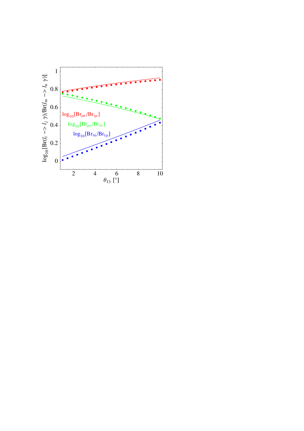
Decoupling of one heavy neutrino and cosmological implications
The supersymmetric seesaw model involves many free parameters. In order to correlate the model predictions for LFV processes one has to resort to some supplementary hypotheses. Here we discuss the consequences of the assumption that one of the heavy singlet neutrinos (not necessarily the heaviest one) decouples from the see-saw mechanism [228].
If the light neutrino masses are hierarchical, in which case the effects of the renormalization group (RG) running [707] of are negligible, at least 3 arguments support this assumption. The first one is the naturalness of the see-saw mechanism. Large mixing angles are not generic for hierarchical light neutrino masses (for a review, see [708]). They are natural only for special patterns of the matrix . One is a large hierarchy between one and the remaining two terms in the sum in (0.3.43) [709, 135, 34, 223]. This is what we call decoupling (one term hierarchically smaller) or dominance (hierarchically larger). Seesaw with only two heavy singlet neutrinos [224, 225] is the limiting case of the decoupling of with and . The immediate consequence of decoupling is ( has rank 2 if there are only 2 terms in the sum in (0.3.43)). Similarly, for dominance one has .
Secondly, decoupling of the lightest singlet neutrino alleviates the gravitino problem of leptogenesis which in the see-saw models of neutrino masses appears to be the most natural mechanism for producing the observed baryon asymmetry of the Universe2020 20 See [279]; for a review of leptogenesis, see [313]; for a discussion of flavour effects in leptogenesis see, e.g. [285]; for recent analyses of the gravitino problem, see, e.g., [710] (BAU). As the Universe cools down leptonic asymmetries (subsequently converted into baryon asymmetry through sphaleron transitions) (where and are the flavour lepton and antilepton number densities, respectively and is the entropy density) are produced in the decays of . The final magnitudes of are proportional to the decay asymmetries , (which in turn are proportional to the heavy neutrino masses) and crucially depend on the processes which wash out the asymmetries generated by the decays. The efficiency of these processes depends on the parameters , where and it is the smallest (i.e. leptogenesis is most efficient) for in the meV range (assuming vanishing density of after re-heating and strongly hierarchical spectrum of ). If it is which is decoupled, there are essentially no lower bounds on and , hence also the re-heating temperature , already of order GeV are sufficient [711, 300] (see, however, e.g., [305]) to reproduce the observed BAU.2121 21 In contrast, for or decoupled, the washout is much stronger and has to be GeV. This requires leading to a much larger dangerous gravitino production [712]. Lower is in this case possible only if and are sufficiently degenerate [713].
Finally, one heavy singlet neutrino must be decoupled if its superpartner, , plays the role of the inflaton field [336]. In such a scenario the (s)neutrino mass must be [338] GeV and the re-heating temperature following inflaton decay is given by . Requiring GeV (the gravitino problem) then implies eV. In this scenario, the leptonic asymmetries must be produced non-thermally in the inflaton decay. Decoupling of is favoured because if it is or which is the inflaton the produced asymmetry may be subsequently washed out during the decays of .
The assumption that effectively decouples from the seesaw mechanism or that effectively dominates the seesaw mechanism translates into one of the following forms of :
| (0.5.45) |
where are complex numbers satisfying and denotes permutation of the rows of . Both conditions can be simultaneously satisfied for , known as sequential dominance (for a review, see, e.g. [714]).
In the framework considered, violation of the leptonic flavour is transmitted from the neutrino Yukawa couplings to the slepton mass matrices through the RG corrections. Branching ratios of LFV decays are well described by a single mass-insertion approximation via Eq. (0.5.27) and Eq. (0.5.28). Since decoupling of is best motivated we discuss the results for LFV only in this case.2222 22 Results for decoupled are the same as for decoupled (including sub-leading effects if takes the numerical value of ). The same is true also for decoupled (including the case with only 2 heavy singlet neutrinos) if is numerically the same as for decoupled . However, if is the inflaton the LFV decays have the rates too low to be observed. In addition, if decouples due to its very large mass its large Yukawa can, for , still dominate the LFV effects which are then practically unconstrained by the oscillation data; some constraints can then be obtained from the limits on the electron EDM [715].
The matrix has then the first of the patterns displayed in Eq. (0.5.45) with . The discussion simplifies if a technical assumption that is made. relevant for then reads:
| (0.5.46) |
where , and . For relevant for we get:
| (0.5.47) |
Analysis of the expressions (0.5.46) and (0.5.47) leads to a number of conclusions [228]. Firstly, the branching ratios of the LFV decays depend (apart from the scales of soft supersymmetry breaking and the value of ) mostly on the mass of the heaviest of the two un-decoupled singlet neutrinos (in this case ). Secondly, for fixed , they depend strongly on the magnitude and phase of , mildly on the undetermined element of the light neutrino mixing matrix and, in addition, on the Majorana phases of which cannot be measured in oscillation experiments [535]. The latter dependence is mild for but can lead to strong destructive interference either in or in decreasing them by several orders of magnitude. The interference effects are seen in Fig. 0.5.22(a) and Fig. 0.5.22(b) where the predicted ranges (resulting from varying the unknown Majorana phases) of are shown as a function of for appropriate for the sneutrino inflation scenario, three different values of arg and for GeV, GeV and , consistent with the dark matter abundance [716]. Results for other values of these parameters can be obtained by appropriate rescalings using (0.5.27). For comparison, for selected values of , we also indicate the ranges of resulting from generic form of the matrix (constrained only by the conditions and and ).


The bulk of the predicted values of shown in Fig. 0.5.22(a) and Fig. 0.5.22(b) exceed the current experimental limit. Since GeV leads to masses of the third generation squarks above 1 TeV, suppressing by increasing the SUSY breaking scale conflicts with the stability of the electroweak scale. Moreover, as discussed in [228] in the scenario considered here generically . Thus the observation with , accessible to future experiments would exclude this scenario.
For completeness, in Fig. 0.5.22(c) we also show predictions for in the case of dominance. is in this case controlled mainly by . Moreover, , while allowing for experimental test of this scenario (cf. [717]). The limits in panels and and or in panel correspond to pure sequential dominance.
In conclusion, the well motivated assumption about the decoupling/dominance of one heavy singlet neutrino significantly constrains the predictions for the LFV processes in supersymmetric model. The forthcoming experiments should be able to verify this assumption and, in consequence, to test an interesting class of neutrino mass models.
Triplet seesaw mechanism and lepton flavour violation
In this subsection we intend to discuss the aspect of low scale LFV in rare decays arising in the context of the triplet seesaw mechanism of Section 0.3.2. We consider both non-SUSY and SUSY versions of it. The flavour structure of the (high-energy) Yukawa matrix of Eq. (0.3.65) is the same as that of the (low-energy) neutrino mass matrix . Therefore, in the triplet seesaw scenario the neutrino mass matrix (containing 9 real parameters), which can be tested in the low-energy experiments, is directly linked to the symmetric matrix (containing also 9 real parameters), modulo the ratio , see Eq. (0.3.68). This feature has interesting implications for LFV [239]. Collider phenomenology of the low scale triplet was discussed in Section 0.5.1 The triplet Lagrangian also induces LFV decays of the charged leptons through the one-loop exchange of the triplet states.

The diagrams relevant for the LFV radiative decays (see \eg[718, 719]) are depicted in \Freffig1:arossi. Denoting , where, are the Majorana phases, those imply the following flavour structure:
| (0.5.48) |
where are family indices. Therefore, the amount of LFV is directly and univocally expressed in terms of the low-energy neutrino parameters. In particular, LFV decays depend only on 7 independent neutrino parameters (there is no dependence on the Majorana phases ). Notice that this simple flavour structure is peculiar of the triplet seesaw case, which represents a concrete and explicit realization of the ‘minimal flavour violation’ hypothesis [526] in the lepton sector [532]. Indeed, according to the latter, the low-energy SM Yukawa couplings are the only source of LFV. This is not generically the case for the seesaw mechanism realized through the exchange of the so-called ‘right-handed’ neutrinos, where the number of independent parameters of the high-energy flavour structures is twice more that of the mass matrix .
Finally, the parametric dependence of the dipole amplitude in \Freffig1:arossi is:
| (0.5.49) |
From the present experimental bound on [173], one infers the bound [comparable limit is obtained from ]. We can push further our discussion considering the relative size of LFV in different family sectors:
| (0.5.50) |
These ratios depend only on the neutrino parameters, while do not depend on details of the model, such as the mass scales , or . By taking the present best fit values of the neutrino masses and mixing angles [720]–[721] provided by the analysis of the experimental data, those ratios can be explicitly expressed as:
| (0.5.51) |
where is the squared-mass difference relevant for the atmospheric (solar) neutrino oscillations. These results hold for and for either hierarchical, quasi-degenerate or inverted hierarchical neutrino spectrum (for more details see [239], [722]). It is immediate to translate the above relations into model-independent predictions for ratios of LFV processes:
| (0.5.52) |
Now we focus upon the supersymmetric version of the triplet seesaw mechanism. (Just recall just that in the supersymmetric case there is only one mass parameter, , while the mass parameter of the non-supersymmetric version is absent from the superpotential and its role is taken by .) Regarding the aspect of LFV, in this case we have to consider besides the diagrams of \Freffig1:arossi also the related ones with each particle in the loop replaced by its superpartner (). Such additional contributions would cancel those in \Freffig1:arossi in the limit of exact supersymmetry. In the presence of soft supersymmetry breaking (SSB) the cancellation is only partial and the overall result for the coefficient of the dipole amplitude behaves like
| (0.5.53) |
which is suppressed with respect to the non-supersymmetric result (0.5.49) for ( denotes an average soft-breaking mass parameter). In the supersymmetric version of the triplet seesaw mechanism flavour violation can also be induced by renormalization effects via Eq. (0.3.71) (the complete set of RGEs of the MSSM with the triplet states have been computed in [239]). Thus in SUSY model the LFV processes can occur also in the case of very heavy triplet. In that case the relevant flavour structure responsible for LFV is again for which we have already noticed its unambiguous dependence on the neutrino parameters in Eq. (0.5.48). Clearly, we find that analogous ratios as in Eq. (0.5.50) hold also for the LFV entries of the soft-breaking parameters, \eg
| (0.5.54) |
Such SSB flavour-violating mass parameters induce extra contributions to the LFV processes. For example, the radiative decays receive also one-loop contributions with the exchange of the charged-sleptons/neutralinos and sneutrinos/charginos, where the slepton masses are the source of LFV. The relevant dipole terms have a parametric dependence of the form
| (0.5.55) |
Notice the inverted dependence on the ratio with respect to the triplet-exchange contribution. Due to this feature, the MSSM sparticle-induced contributions (0.5.55) tends to dominate over the one induced by the triplet-exchange. In this case, analogous ratios as in (0.5.52) can be derived, \ie
| (0.5.56) |
(For more details see [239].)
The presence of extra triplet states at intermediate energy spoils the successful gauge coupling unification of the MSSM. A simple way to recover gauge coupling unification is to introduce more states , to complete a certain representation – such that – of some unifying gauge group , . In general the Yukawa couplings of the states are related to those of the triplet partners . Indeed, this is generally the case in minimal GUT models. In this case RG effects generates not only lepton- flavour violation but also closely correlated flavour violation in the quark sector (due to the -couplings). An explicit scenario with where both lepton and quark flavour violation arise from RG effects was discussed in ??[239]. In Section 0.5.3 we review a supersymmetric model for the triplet seesaw scenario.
0.5.3 SUSY GUTs
Flavour violation in the minimal supersymmetric SU(5) seesaw model
In this section we review flavor- and/or CP-violating phenomena in the minimal SUSY SU(5) GUT, in which the right-handed neutrinos are introduced to generate neutrino masses by the type-I seesaw mechanism. Here, it is assumed that the Higgs doublets in this MSSM are embedded in 5- and - dimensional SU(5) multiplets. Rich flavor structure is induced even in those minimal particle contents. The flavor-violating SUSY breaking terms for the right-handed squarks and sleptons are generated by the GUT interaction, while those are suppressed in the MSSM (+) under the universal scalar mass hypothesis for the SUSY breaking terms.
The Yukawa interactions for quarks and leptons and the Majorana mass terms for the right-handed neutrinos in this model are given by the following superpotential,
| (0.5.57) |
where and are for 10- and -dimensional multiplets, respectively, and is for the right-handed neutrinos. () is 5- (-) dimensional Higgs multiplets. After removing the unphysical degrees of freedom, the Yukawa coupling constants in Eq. (0.5.57) are given as follows,
| (0.5.58) |
Here, denote diagonal Yukawa couplings, and – are CP-violating phases inherent in the SUSY SU(5) GUT (). The unitary matrix is the CKM matrix in the extension of the SM to the SUSY SU(5) GUT, and each unitary matrices and have only a phase. When the Majorana mass matrix for the right-handed neutrinos is real and diagonal in the basis of Eq. (0.5.58), is the PMNS matrix measured in the neutrino oscillation experiments and the light neutrino mass eigenvalues are given as , in which are the diagonal components.
The colored-Higgs multiplets and are introduced in and as SU(5) partners of the Higgs doublets and in the MSSM, respectively, and they have new flavor-violating interactions. Eq. (0.5.57) is represented by the fields in the MSSM as follows,
| (0.5.59) | |||||
Here, the superpotential in the MSSM with the right-handed neutrinos is
| (0.5.60) | |||||
The flavor-violating interactions, which are absent in the MSSM, emerge in the SUSY SU(5) GUT due to existence of the colored-Higgs multiplets. The colored-Higgs interactions are also baryon-number violating [361, 145], and then proton decay induced by the colored-Higgs exchange is a serious problem, especially in the minimal SUSY SU(5) GUT [364]. However, the constraint from the proton decay depends on the detailed structure in the Higgs sector, and it is also loosened by global symmetries, such as the Peccei-Quinn symmetry and the U(1)R symmetry. Thus, we may ignore the constraint from the proton decay while we adopt the minimal Yukawa structure in Eq. (0.5.57).
The sfermion mass terms get sizable corrections by the colored-Higgs interactions, when the SUSY-breaking terms in the MSSM are generated by dynamics above the colored-Higgs masses. In the minimal supergravity scenario the SUSY breaking terms are supposed to be given at the reduced Planck mass scale (). In this case, the flavor-violating SUSY breaking mass terms at low energy are induced by the radiative correction, and they are qualitatively given in a flavor basis as
| (0.5.61) |
with , where and and is the colored-Higgs mass. Here, is the SUSY-breaking scale in the MSSM, and are the universal scalar mass and trilinear coupling, respectively, in the minimal supergravity scenario. is the top quark Yukawa coupling constant while is for the bottom quark. The off-diagonal components in the right-handed squarks and slepton mass matrices are induced by the colored-Higgs interactions, and they depend on the CP-violating phases in the SUSY SU(5) GUT with the right-handed neutrinos [723].
One of the important features of the SUSY GUTs is the correlation between the leptonic and hadronic flavor violations [724, 725]. From Eq. (0.5.61), we get a relation
| (0.5.62) |
The right-handed bottom-strange squark mixing may be tested in the factory experiments since it affects mixing, CP asymmetries in the penguin processes such as , and the mixing-induced CP asymmetry in . (See Chapter 2.) The relation in Eq. (0.5.62) implies that the deviations from the standard model predictions in the - transition processes are correlated with in the SUSY SU(5) GUT. We may test the model in the factories.
In \Freffig1_MSGUTN we show the CP asymmetry in () and as an example of the correlation. Here, we assume the minimal supergravity hypothesis for the SUSY breaking terms. See the caption and Ref. [724] for the input parameters and the details of the figure. It is found that and are correlated and a large deviation from the standard model prediction for is not possible due to the current bound on in the SUSY SU(5) GUT.

In Eq. (0.5.61), we take the SU(5)-symmetric Yukawa interactions given in Eq. (0.5.57), while they fails to explain the fermion mass relations in the first and second generations. We have to extend the minimal model by introducing non-trivial Higgs or matter contents or the higher-dimensional operators including SU(5)-breaking Higgs field. These extensions may affect the prediction for the sfermion mass matrices. However, the relation in Eq. (0.5.62) is rather robust when the neutrino Yukawa coupling constant of the third generation is as large as those for the top and bottom quarks and the large mixing in the atmospheric neutrino oscillation comes from the lopside structure of the neutrino Yukawa coupling.
Another important feature of the SUSY GUTs is that both the left- and right-handed squarks and sleptons have flavor mixing terms. In this case, the hadronic and leptonic electric dipole moments (EDMs) are generated due to the flavor violation, and they may be large enough to be observed in the future EDM measurements [726]. A diagram in \Freffig2_MSGUTN(a) generates the electron EDM even at one-loop level, when the relative phase between the left- and right-handed slepton mixing terms is non-vanishing. While this contribution is suppressed by the flavor violation, it is compensated by a heavier fermion mass, that is, . Similar diagrams in \Freffig2_MSGUTN(b) contribute to quark EDMs and chromo-electric dipole moments (CEDM), which induce the hadronic EDMs. The EDM measurements are important to probe the interaction of the SUSY SU(5) GUT.


In \Freffig3_MSGUTN the CEDMs for strange () and down quarks () are shown as functions of the right-handed tau neutrino mass in the SUSY SU(5) GUT with the right-handed neutrinos. See the caption and Ref. [727] for the input parameters. The mercury atom EDM, which is a diamagnetic atom, is sensitive to quark CEDMs via the nuclear force, while the neutron EDM depends on them in addition to the quark EDMs. (The evaluation of the hadronic EDMs from the effective operators at the parton level is reviewed in Section 9.1 and also Ref. [728].) The strange quark contribution to the mercury atom EDM is suppressed by the strange quark mass. On the other hand, it is argued in Refs. [729, 730] that the strange quark component in nucleon is not negligible and the strange quark CEDM may give a sizable contribution to the neutron EDM. It implies that we may probe the different flavor mixings by measurements of the various hadronic EDMs, though the evaluation of the hadronic EDMs still has large uncertainties.
It is argued that the future measurements of neutron and deuteron EDMs may reach to levels of and , respectively. When the sensitivity of deuteron EDM is established, we may probe the new physics to the level of and [836]. The future measurements for the EDMs will give great impacts on the SUSY SU(5) GUT with the right-handed neutrinos.


LFV in the minimal GUT with triplet seesaw
In this Section we discuss phenomenology of the minimal GUT which incorporates the triplet seesaw mechanism, previously presented in Sections 0.3.2 and 0.5.2. Review of more general class of GUT models also including triplet Higgs has been given in Section 0.4.1. In GUTs based on there is no natural place for incorporating singlet neutrinos, From this point of view presents some advantage for implementing the triplet seesaw mechanism. In particular, a very predictive scenarios can be obtained in the supersymmetric case [239, 731, 722]. The triplet states () fit into the 15 representation, with , and transforming as under (the decomposition is obvious). We will briefly show that it is also possible to relate not only neutrino mass parameters and LFV (as shown in Section 0.5.2) but also sparticle and Higgs spectra and electroweak symmetry breakdown [731, 722]. For this purpose, consider that the model conserves , so that the relevant superpotential reads:
| (0.5.63) |
where the multiplets are understood as , and the Higgs doublets fit with their coloured partners and , like and is a singlet superfield. The quantum numbers are the combination where are the hypercharges and . Both the scalar and auxiliary components of the superfield are assumed to acquire a VEV through some unspecified dynamics in the hidden sector. Namely, while only breaks , breaks both SUSY and . These effects are parameterized by the superpotential mass term , where , and the bilinear SSB term , with . The and states act, therefore, as messengers of both and SUSY breaking to the MSSM observable sector. Once is broken to the SM group we find, below the GUT scale ,
| (0.5.64) |
Here, denotes the MSSM superpotential 2323 23 This should be regarded as an effective approach where the Yukawa matrices include -breaking effects needed to reproduce a realistic fermion spectrum., the term is responsible for neutrino mass generation [cf. (0.3.69)], while the couplings and masses of the coloured fragments and are included in . It is also understood that . At the decoupling of the heavy states we obtain at tree-level the neutrino masses, given by Eq. (0.3.70) and at the quantum level all SSB mass parameters of the MSSM via gauge and Yukawa interactions. At one-loop level, only the trilinear scalar couplings, the gaugino masses and the Higgs bilinear mass term are generated:
| (0.5.65) |
The scalar mass matrices instead are generated at the two-loop level and receive both gauge-mediated contributions proportional to ( is the quadratic Casimir of the -particle) and Yukawa-mediated ones of the form . The former piece is the flavour blind contribution, which is proper of the gauge-mediated scenarios [732, 733, 146, 734, 735, 736, 737, 147], while the latter ones constitute the flavour violating contributions transmitted to the SSB terms by the Yukawa’s . These contributions are mostly relevant for the mass matrices and . For example,
| (0.5.66) | |||||
Since the flavour structure of is proportional to (and to which is -related to ), it can be expressed in terms of the neutrino parameters [cf. Eq. (0.3.70)] and so the relative size of LFV in different leptonic families is predicted according to the results of Eq. (0.5.54).


| prediction for branching ratio | ||
|---|---|---|
| decay mode | ||
All the soft masses have the same scaling behaviour which demands to fulfill the naturalness principle. This scenario appears very predictive since it contains only three free parameters: the triplet mass , the effective SUSY breaking scale and the coupling constant . The parameter space is then constrained by the experimental bounds on the Higgs boson mass, the , the sfermion masses, and the requirement of radiative electroweak symmetry breaking. The phenomenological predictions more important and relevant for LHC, the B-factories [681] the incoming MEG experiment [538], the Super Flavour factory [738] or the PRISM/PRIME experiment at J-PARC [739], concern the sparticle and Higgs boson spectra and the LFV decays. Regarding the spectrum, the gluino is the heaviest sparticle while, in most of the parameter space, is the lightest. In the example shown in Fig.0.5.27 the squark and slepton masses lie in the ranges 700–950 GeV and 100 – 300 GeV, respectively. The gluino mass is about 1.3 TeV. The chargino masses are GeV and GeV. Moreover, GeV, and . These mass ranges are within the discovery reach of the LHC.
The Higgs sector is characterized by a decoupling regime with a light SM-like Higgs boson () with mass in the range which is testable in the near future at LHC (mainly through the decay into 2 photons). The remaining three heavy states ( and ) have mass GeV (again, for TeV). All the spectra increase almost linearly with .
Figure 0.5.28b shows instead several LFV processes: , conversion in nuclei, and , . One observe that \egthe behaviour of the radiative-decay branching ratios is in agreement with the estimates given in Eq. (0.5.56) for . For one obtains instead that and (the full analysis can be found in ??[722]). The other LFV processes shown are also correlated to the radiative ones in a model-independent way [731, 722]. The analysis shows that the future experimental sensitivity will allow to measure at most , , and CR( Ti) for tiny . In particular, being , is expected not to exceed , irrespective of the type of neutrino spectrum. Therefore falls into the LHC capability. All the decays would have . The predictions for the LFV branching ratios in the present scenario are summarized in Table 0.5.4.
LFV from a generic SO(10) framework
The spinorial representation of the , given by a 16-dimensional spinor, can accommodate all the SM model particles as well as the right handed neutrino. As discussed in Section 0.4.1, the product of two 16 matter representations can only couple to 10, 120 or 126 representations, which can be formed by either a single Higgs field or a non-renormalizable product of representations of several Higgs fields. In either case, the Yukawa matrices resulting from the couplings to 10 and 126 are complex-symmetric, whereas they are antisymmetric when the couplings are to the 120. Thus, the most general superpotential relevant to fermion masses can be written as
| (0.5.67) |
where refer to the generation indices. In terms of the SM fields, the Yukawa couplings relevant for fermion masses are given by [742, 743]:
| (0.5.68) | |||||
where we have specified the corresponding Higgs representations for each of the couplings and all the fermions are left handed fields. The resulting up-type quarks and neutrinos’ Dirac mass matrices can be written as:
| (0.5.69) | |||||
| (0.5.70) |
A simple analysis of the fermion mass matrices in the model, as detailed in the Eq. (0.5.70) leads us to the following result: At least one of the Yukawa couplings in has to be as large as the top Yukawa coupling [159]. This result holds true in general, independently of the choice of the Higgses responsible for the masses in Eqs. (0.5.69), (0.5.70), provided that no accidental fine-tuned cancellations of the different contributions in Eq. (0.5.70) are present. If contributions from the 10’s solely dominate, and would be equal. If this occurs for the 126’s, then [385]. In case both of them have dominant entries, barring a rather precisely fine-tuned cancellation between and in Eq. (0.5.70), we expect at least one large entry to be present in . A dominant antisymmetric contribution to top quark mass due to the 120 Higgs is phenomenologically excluded, since it would lead to at least a pair of heavy degenerate up quarks. Apart from sharing the property that at least one eigenvalue of both and has to be large, for the rest it is clear from Eqs. (0.5.69) and (0.5.70) that these two matrices are not aligned in general, and hence we may expect different mixing angles appearing from their diagonalization. This freedom is removed if one sticks to particularly simple choices of the Higgses responsible for up quark and neutrino masses.
Therefore, we see that the model with only two ten-plets would inevitably lead to small mixing in . In fact, with two Higgs fields in symmetric representations, giving masses to the up-sector and the down-sector separately, it would be difficult to avoid the small CKM-like mixing in . We will call this case the CKM case. From here, the following mass relations hold between the quark and leptonic mass matrices at the GUT scale2424 24 Clearly this relation cannot hold for the first two generations of down quarks and charged leptons. One expects, small corrections due to non-renormalizable operators or suppressed renormalizable operators [2] to be invoked.:
| (0.5.71) |
In the basis where charged lepton masses are diagonal, we have
| (0.5.72) |
The large couplings in induce significant off-diagonal entries in through the RG evolution between and the scale of the right-handed Majorana neutrinos, . The induced off-diagonal entries relevant to are of the order of:
| (0.5.73) |
where are elements of , and , flavour indices. In this expression, the CKM angles are small but one would expect the presence of the large top Yukawa coupling to compensate such a suppression. The required right-handed neutrino Majorana mass matrix, consistent with both the observed low energy neutrino masses and mixing as well as with CKM-like mixing in is easily determined from the seesaw formula defined at the scale of right-handed neutrinos.

The are now predictable in this case. Considering mSUGRA boundary conditions and taking , we obtain that reaching a sensitivity of , as planned by the MEG experiment at PSI, for would allow us to probe the SUSY spectrum completely up to (notice that this corresponds to gluino and squark masses of order 1 TeV). This clearly appears from Fig. 0.5.29, which shows the contour plot in the plane. Thus, in summary, though the present limits on would not induce any significant constraints on the supersymmetry-breaking parameter space, an improvement in the limit to , as foreseen, would start imposing non-trivial constraints especially for the large region.
To obtain mixing angles larger than CKM angles, asymmetric mass matrices have to be considered. In general, it is sufficient to introduce asymmetric textures either in the up-sector or in the down-sector. In the present case, we assume that the down-sector couples to a combination of Higgs representations (symmetric and antisymmetric)2525 25 The couplings of the Higgs fields in the superpotential can be either renormalizable or non-renormalizable. See [744] for a non-renormalizable example. , leading to an asymmetric mass matrix in the basis where the up-sector is diagonal. As we will see below, this would also require that the right-handed Majorana mass matrix be diagonal in this basis. We have :
where the 126, as before, generates only the right-handed neutrino mass matrix. To study the consequences of these assumptions, we see that at the level of , we have
where we have decomposed the into and and are components of and respectively. To have large mixing in we see that the asymmetric matrix should now give rise to both the CKM mixing as well as PMNS mixing. This is possible if
| (0.5.74) |


Therefore the that contains the left-handed down-quarks would be rotated by the CKM matrix whereas the that contains the left-handed charged leptons would be rotated by the matrix to go into their respective mass bases [745, 723, 746, 744]. Thus we have the following relations in the basis where charged leptons and down quarks are diagonal:
| (0.5.75) | |||||
| (0.5.76) |
Using the seesaw formula of Eqs. (0.3.43) and (0.5.76), we have
| (0.5.77) |
We now turn our attention to lepton flavour violation in this case. The branching ratio, would now depend on
| (0.5.78) |
It is clear from the above that in contrast to the CKM case, the dominant contribution to the off-diagonal entries depends on the unknown magnitude of the element [747]. If is close to its present limit [748] (or at least larger than ), the first term on the RHS of the Eq. (0.5.78) would dominate. Moreover, this would lead to large contributions to the off-diagonal entries in the slepton masses with of . Thus, we have
| (0.5.79) |
This contribution is larger than the CKM case by a factor of . This would mean about a factor times larger than the CKM case in B(. Such enhancement with respect to the CKM case is clearly shown in the scatter plots of Fig. 0.5.30, where the CKM case is compared with the PMNS case with . The aim of the figure is to show the capability of MEG to probe the region of mSUGRA parameter space accessible to the LHC. In fact, the plots show the value of B( obtained by scanning the parameter space in the large region ( TeV, TeV, , sign()), and then keeping the points which give at least one squark lighter than 2.5 TeV (so roughly accessible to the LHC). We see that in this “LHC accessible” region the maximal case (with ) is already excluded by the MEGA limit (), and therefore MEG will constrain the parameter space far beyond the LHC sensitivity for this case. If is very small, i.e either zero or , the second term in Eq. (0.5.78) would dominate, thus giving a strong suppression to the branching ratio. This could be not true, once RG effects on itself [707, 248] are taken into account. The point is that the PMNS boundary condition (0.5.76) is valid at high scale. Thus, it is necessary to evolve the neutrino masses and mixing from the low-energy scale, where measurements are performed, up to high energy. Such effect turns out to be not negligible in case of low-energy , giving a high-energy constant enhancement of order [676]. The consequence is that the term in Eq. (0.5.78) always dominates, giving a contribution to the branching ratio larger than the CKM case (which turns out to be really a “minimal” case) and bringing the most of the parameter space in the realm of MEG even for very small low-energy values of [676, 749].
The transitions are instead -independent probes of SUSY, whose importance was first pointed out in Ref. [717]. The off-diagonal entry in this case is given by :
| (0.5.80) |
In the decay the situation is at the moment similarly constrained with respect to , if happens to be very small. The main difference is that B() does not depend on the value of , so that will be a promising complementary channel with respect to . As far as Beauty factories [750, 632, 184] are concerned, we see from Fig. 0.5.30, that even with the present bound it is possible to rule out part of LHC accessible region in the PMNS high regime; the planned accuracy of the SuperKEKB [681] machine will allow to test much of high region and will start probing the low PMNS case, with a sensitivity to soft masses as high as GeV. The situation changes dramatically if one takes into account the possibility of a Super Flavour factory: taking the sensitivity of the most promising process to , the PMNS case will be nearly ruled out in the high regime and severely constrained in the low one; as for the CKM case we would enter the region of interest.
Let’s finish with some remarks. Suppose that the LHC does find signals of low-energy supersymmetry, then grand unification becomes a very appealing scenario, because of the successful unification of gauge couplings driven by the SUSY partners. Among SUSY-GUT models, an framework is much favored as it is the ‘minimal’ GUT to host all the fermions in a single representation and it accounts for the smallness of the observed neutrino masses by naturally including the see-saw mechanism. In the above we have addressed the issue by a generic benchmark analysis, within the ansatz that there is no fine-tuning in the neutrino Yukawa sector. We can state that LFV experiments should be able to tell us much about the structure of such a SUSY-GUT scenario. If they detect LFV processes, by their rate and exploiting the interplay between different experiments, we would be able to get hints of the structure of the unknown neutrinos’ Yukawa’s. On the contrary, in the case that both MEG and a future Super Flavour factory happen not to see any LFV process, only two possibilities should be left: (i) the minimal mixing, low scenario; (ii) mSUGRA see-saw without fine-tuned couplings is not a viable framework of physics beyond the standard model.
Actually one should remark that LFV experiments will be able to falsify some of above scenarios even in regions of the mSUGRA parameter space that are beyond the reach of LHC experiments. In this sense, the power of LFV experiments of testing/discriminating among different SUSY-GUTs models results very interesting and highly complementary to the direct searches at the LHC.
LFV, QFV and CPV observables in GUTs and their correlations
In a SUSY Grand Unified Theory (GUT), quarks and leptons sit in same multiplets and are transformed ones into the others through GUT symmetry transformations. If the energy scale where the SUSY breaking terms are transmitted to the visible sector is larger then the GUT scale, as in the case of gravity mediation, such breaking terms, and in particular the sfermion mass matrices, will have to respect the underlying GUT symmetry. Hence, as already discussed in Section 0.5.3, the quark-lepton unification seeps also into the SUSY breaking soft sector. If the soft SUSY breaking terms respect boundary conditions which are subject to the GUT symmetry to start with, we generally expect the presence of relations among the (bilinear and trilinear) scalar terms in the hadronic and leptonic sectors [725, 160]. Such relations hold true at the (superlarge) energy scale where the correct symmetry of the theory is the GUT symmetry. After its breaking, the mentioned relations will undergo corrections which are computable through the appropriate RGE’s which are related to the specific structure of the theory between the GUT and the electroweak scale (for instance, new Yukawa couplings due to the presence of RH neutrinos acting down to the RH neutrino mass scale, presence of a symmetry breaking chain with the appearance of new symmetries at intermediate scales, etc.). As a result of such a computable running, we can infer the correlations between the softly SUSY breaking hadronic and leptonic MIs at the low scale where FCNC tests are performed. Moreover, given that a common SUSY soft-breaking scalar term of at scales close to can give rise to RG-induced ’s and ’s at the weak scale, one may envisage the possibility to make use of the FCNC constraints on such low-energy ’s to infer bounds on the soft breaking parameters of the original supergravity Lagrangian (). Indeed, for each scalar soft parameter of one can ascertain whether the hadronic or the leptonic corresponding bound at the weak scale yields the strongest constraint at the large scale [160].
Let us consider the scalar soft breaking sector of the MSSM:
| (0.5.81) | |||||
where we have explicitly written down the various off-diagonal entries of the soft SUSY breaking matrices. Consider now that is the relevant symmetry at the scale where the above soft terms firstly show up. Then, taking into account that matter is organized into the representations and , one obtains the following relations
| (0.5.82) |
These equations for matrices in flavour space lead to relations between the slepton and squark flavour violating off-diagonal entries . These are:
| (0.5.83) | |||
| (0.5.84) | |||
| (0.5.85) |
These GUT correlations among hadronic and leptonic scalar soft terms are summarized in the second column of Table 0.5.5. Assuming that no new sources of flavour structure are present from the scale down to the electroweak scale, apart from the usual SM CKM one, one infers the relations in the first column of Table 0.5.5 at low scale. Here we have taken into account that due to their different gauge couplings “average” (diagonal) squark and slepton masses acquire different values at the electroweak scale.
| Relations at weak-scale | Boundary conditions at |
|---|---|
Two comments are in order when looking at Table 0.5.5. First, the boundary conditions on the sfermion masses at the GUT scale (last column in Table 0.5.5) imply that the squark masses are always going to be larger at the weak scale compared to the slepton masses due to the participation of the QCD coupling in the RGEs. As a second remark, notice that the relations between hadronic and leptonic MI in Table 0.5.5 always exhibit opposite “chiralities”, i.e. LL insertions are related to RR ones and vice-versa. This stems from the arrangement of the different fermion chiralities in five- and ten-plets (as it clearly appears from the final column in Table 0.5.5). This restriction can easily be overcome if we move from to left-right symmetric unified models like or the Pati-Salam (PS) case (we exhibit the corresponding GUT boundary conditions and MI at the electroweak scale in Table 0.5.6).
| Relations at weak-scale | Boundary conditions at |
|---|---|
So far we have confined the discussion within the simple model, without the presence of any extra particles like right handed (RH) neutrinos. In the presence of RH neutrinos, one can envisage of two scenarios [159]: (a) with either very small neutrino Dirac Yukawa couplings and/or very small mixing present in the neutrino Dirac Yukawa matrix, (b) Large Yukawa and large mixing in the neutrino sector. In the latter case, Eqs. (0.5.83 – 0.5.85) are not valid at all scales in general, as large RGE effects can significantly modify the sleptonic flavour structure while keeping the squark sector essentially unmodified; thus essentially breaking the GUT symmetric relations. In the former case where the neutrino Dirac Yukawa couplings are tiny and do not significantly modify the sleptonic flavour structure, the GUT symmetric relations are expected to be valid at the weak scale. However, in both cases it is possible to say that there exists a bound on the hadronic parameters of the form [725]:
| (0.5.86) |
The situation is different if we try to translate the bound from quark to lepton MIs. An hadronic MI bound at low energy leads, after RGE evolution, to a bound on the corresponding grand-unified MI at , applying both to slepton and squark mass matrices. However, if the neutrino Yukawa couplings have sizable off-diagonal entries, the RGE running from to could still generate a new contribution to the slepton MI that exceeds this GUT bound. Therefore hadronic bounds cannot be translated to leptons unless we make some additional assumptions on the neutrino Yukawa matrices. On general grounds, given that SM contributions in the lepton sector are absent and that the branching ratios of leptonic processes constrain only the modulus of the MIs, it turns out that all the MI bounds arising from the lepton sector are circles in the – plane and are centered at the origin.


In the following the effect of leptonic bounds on the quark mass insertions are reviewed, following the results presented in [160], where constraints on s were studied scanning the mSUGRA parameter space in the ranges: GeV, GeV, and . For instance, in presence of a at the GUT scale, this would have effects both in the and decays. Using , a bound on from the decay translates into a bound on (neglecting the effects of neutrino Yukawa’s the inequality transforms into equality). Thus, leptonic processes set a bound on the SUSY contributions to . However, it turns out that the present leptonic bounds have no effect on the couplings. This is due both to the existence of strong hadronic bounds from and CP asymmetries and to the relatively weak leptonic bounds here.
Similarly, in presence of a at the GUT scale, the corresponding MIs at the electroweak scale are and that contribute to and respectively (the impact of on and is not relevant because of the absence of interference between SUSY and SM contributions). In Fig. 0.5.31 the allowed values of and with the different constraints are shown. The leptonic constraints are quite effective as the bound on the from B-factories is already very stringent, while the recent measurement of is less constraining. The plots correspond to , thus, the absolute bound on is set by and it scales with as 2626 26 Sizable SUSY contributions to are still possible from the Higgs sector in the large regime both within [751, 752, 753] and also beyond [754] the Minimal Flavor Violating framework. However, for the considered parameter space, the above effects are completely negligible..
As in the LR sector, in the LL one, there is no appreciable improvement from the inclusion of leptonic constraints. In fact, is not effective to constrain , i.e. the leptonic MI related to in this SUSY-GUTs scheme, in large portions of the parameter space because of strong cancellations among amplitudes. The analysis of the constraints on the different MIs gives similar results to that of the MIs. In this case, the hadronic constraints come mainly from and the different CP asymmetries measured at B-factories, while the leptonic bounds are due to the decay .
Coming to the 1-2 sector, let’s see, as an example, the allowed values of and . In this case, as it appears from Fig. 0.5.31, leptonic constraints, already using the present limit on , are competitive and constrain the direction in which the constraint from is not effective (upper left plot). Similarly in the LR sector, even if the hadronic bounds coming from are quite stringent, the bounds from are even more effective, while the LL sector results less constrained by leptonic processes, as an effect of the cancellations that decay suffers in the RR leptonic sector.
0.5.4 R-parity violation
Introduction
In supersymmetric extensions of the Standard Model (SM), baryon and lepton numbers are no longer automatically protected. This is the main reason for introducing -parity. -parity is associated with a subgroup of the group of continuous transformations acting on the gauge superfields and the two chiral doublet Higgs superfields and , with their definition extended to quark and lepton superfields so that quarks and leptons carry and squarks and sleptons . One can express -parity in terms of spin , baryon and lepton number [755]:
| (0.5.87) |
Taking into account the important phenomenological differences between models with and without -parity, it is worth studying if and how -parity can be broken. One of the main reasons to introduce R-parity is avoiding proton decay. However there are in principle other discrete or continuous symmetries that can protect proton decay while allowing for some -parity violating couplings. In the absence of -parity, -parity odd terms allowed by renormalizability and gauge invariance [145] must be included in the superpotential of the Minimal Supersymmetric Standard Model,
| (0.5.88) |
where there is summation over the generation indices , and summation over gauge indices is understood. One has for example and , where are indices, are indices, and and are totally antisymmetric tensors (with ). Gauge invariance enforces antisymmetry of the couplings in their first two indices and antisymmetry of the couplings in their last two indices,
| (0.5.89) | |||||
| (0.5.90) |
The bilinear terms in Eq. (0.5.88) can be rotated away from the superpotential upon suitably redefining the lepton and Higgs superfields. However, in the presence of generic soft supersymmetry breaking terms of dimension two, bilinear -parity violation will reappear. The fact that one can make in Eq. (0.5.88) does not mean that the Higgs-lepton mixing associated with bilinear -parity breaking is unphysical, but rather that there is not a unique way of parameterizing it. If R-parity is violated in the leptonic sector, no quantum numbers differentiate between lepton and Higgs superfields, and they consequently mix with each other [756]. The R-parity violation in the baryonic sector does not imply lepton flavour violation, and we do not consider such option here.
A general consequence of -parity violation is that unless the relevant couplings are negligibly small, the supersymmetric model does not have a dark matter candidate. Thus experimental studies on dark matter will also shed light on -parity violation.
Limits on couplings
Limits on -parity violating couplings can be obtained by direct searches at colliders or requiring that the -parity violating contribution to a given observable does not exceed the limit imposed by the precision of the experimental measurement.
On the collider side -parity violation implies the possibility of the creation, decay or exchange of single sparticles, thus allowing new decay channels. For example, even for relatively small -parity violating interactions, the decay of the lightest supersymmetric particle will lead to collider events departing considerably from the characteristic missing momentum signal of -parity conserving theories. In absence of definite theoretical predictions for the values of the 45 independent trilinear Yukawa couplings (, and ), it is necessary in practice to assume a strong hierarchy among the couplings. A simplifying assumption widely used for the search at colliders is to postulate the existence of a single dominant -parity violating coupling. When discussing specific bounds, it is necessary to choose a definite basis for quark and lepton superfields. Often it is understood that the single coupling dominance hypothesis applies in the mass eigenstate basis. It can be more natural to apply this hypothesis in the weak eigenstate basis when dealing with models in which the hierarchy among couplings originates from a flavour theory. In this case, a single process allows to constrain several couplings, provided one has some knowledge of the rotations linking the weak eigenstate and mass eigenstate bases. Indirect bounds from loop processes typically lead to bounds on the products of two most important -parity violating couplings, or on the sum of products of two couplings. The limits on single dominant couplings, and on products of couplings, as well as a more complete list of references, are collected in [757].
Spontaneous -parity breaking
The spontaneous breaking of -parity is characterized by an -parity invariant Lagrangian leading to non-vanishing VEVs for some -parity odd scalar field, which in turn generates -parity violating terms. Such a spontaneous breakdown of -parity generally also entails the breaking of the global lepton number symmetry which implies the existence of a massless Nambu-Goldstone real pseudoscalar boson , the Majoron. Another light scalar particle, denoted , generally accompanies the Majoron in the supersymmetric models. If the symmetry is also explicitly broken by interaction terms in the Lagrangian, both of these particles acquire finite masses. The most severe constraints on the models with a spontaneous -parity breaking, arise in the cases where the Majoron carries electroweak gauge charges and hence is coupled to the bosons and to quarks and leptons. The non-singlet components contribute to the boson invisible width by an amount of one-half that a single light neutrino, MeV. To suppress the non-singlet components one must allow either for sufficiently small sneutrino VEVs, , or for some large hierarchy of scales between and the VEV parameters associated with additional electroweak singlet scalar fields [758].
However, it is not necessary that models with spontaneous -parity violation have a Majoron. Models without a Majoron include a class of models with triplet Higgses, where is a gauge symmetry, which is necessarily spontaneously broken unless effects of non-renormalizable terms or some additional new fields are included [759]. An interesting experimental signal in these models may be a relatively light doubly charged scalar, which decays dominantly to same charge leptons (not necessarily of the same generation) [760]. Another possibility for a model without a Majoron is a model where the lepton number is broken by two units explicitly, in which case the spontaneous breaking by one unit (which breaks the -parity) does not lead to a Majoron [761]. The interactions in spontaneously -parity breaking models through the lepton number violation closely resemble explicitly -parity breaking models with only bilinear -parity violation. In the case of spontaneous breaking, the parameters which are free in the model with only bilinear couplings are related to each other via the sneutrino vacuum expectation value (VEV). Thus a constraint from one process affects availability of the other processes. Example bounds for such a model can be found in [762].
It is worth emphasizing that choosing single coupling dominance in the case of spontaneous breaking is not possible and in this sense, the models with spontaneous breaking are more predictive than those without.
Neutrino sector
The presence of non-zero couplings , or bilinear -parity violating parameters implies the generation of neutrino masses and mixing [763]. This is an interesting feature of -parity violating models, but it can also be a problem, since the contribution of -parity violating couplings may exceed by orders of magnitude the experimental bounds. Two types of contributions can be distinguished: tree-level or loop contributions.
The tree-level contributions are due to bilinear -parity violation terms which induce a mixing between neutrinos and neutralinos [764]. This gives a massive neutrino state at tree level. When quantum corrections are included, all three neutrinos acquire a mass. The tree-level contribution arising from the neutrino-neutralino mixing can be understood, in the limit of small neutrino-neutralino mixing, as a sort of seesaw mechanism, in which the neutral gauginos and Higgsinos play the rôle of the right-handed neutrinos.
The loop contributions are induced by the trilinear -parity violating couplings and and by bilinear -parity violating parameters [765]. If bilinear -parity violation is strongly suppressed one can concentrate on the diagrams involving trilinear -parity violating couplings only. The trilinear couplings and contribute to each entry of the neutrino mass matrix through the lepton-slepton and quark-squark loops. The neutrino mass matrix depends therefore on a large number of trilinear -parity violating couplings. In order to obtain a predictive model, one has to make assumptions on the structure of the trilinear couplings. In general, however, the bilinear -parity violation contribution cannot be neglected. The presence of bilinear terms drastically modifies the calculation of one-loop neutrino masses. The neutrino mass matrix receives contributions already at tree level, as discussed above, and moreover in addition to the lepton-slepton and quark-squark loops, one-loop diagrams involving insertions of bilinear -parity violating masses or slepton VEVs must be considered. One should note that the bilinear -parity violating terms, if not suppressed, give too large loop contributions to neutrino masses.
The scenario known as bilinear R-Parity violation (BRpV) corresponds to the explicit introduction of the three mass parameters in the first term in Eq. (0.5.88), without referring to their origin, and assuming that all the trilinear parameters are zero. The terms introduce tree-level mixing between the Higgs and lepton superfields. Therefore, they violate R-Parity and lepton number, and contribute to the breaking of the symmetry by the induction of sneutrino vacuum expectation values . As it was mentioned before, the mixing between neutralinos and neutrinos leads to an effective tree-level neutrino mass matrix of the form,
| (0.5.91) |
where the parameters are proportional to the sneutrino vacuum expectation values in the basis where the terms are removed from the superpotential. Due to the symmetry of this mass matrix, only one neutrino acquires a mass. Once quantum corrections are included, this symmetry is broken, and the effective neutrino mass matrix takes the form [766],
| (0.5.92) |
If the tree-level contribution dominates, as for example in SUGRA models with low values of , the atmospheric mass scale is given at tree level, and the solar mass scale is generated at one loop, explaining the hierarchy between them. Most of the time, the dominant loop in SUGRA is the one formed with bottom quarks and squarks, followed in importance by loops with charginos and neutralinos. In the tree-level dominance case the atmospheric mixing angle is well approximated by , and the reactor angle by . In this case, the smallness of the reactor angle is achieved with a small value of , and the maximal mixing in the atmospheric sector with a similar value for and . Supergravity scenarios where tree-level contribution does not dominate can also be found [767], in which case the previous approximations for the angles are not valid.
Lepton flavour violating processes at low energies
Many processes, which are either rare or forbidden in the R-parity conserving model, become possible when interactions following from the superpotential in (0.5.88) are available. These interactions include tree-level couplings between different lepton or quark generations, as well as tree-level couplings between leptons and quarks, or leptons and Higgses.
In addition to the trilinear couplings and , bilinear couplings or spontaneous R-parity breaking contribute to the lepton flavour violating processes mentioned below through mixing.
For references about this section, see Ref. [757].
- •
, , and -conversion, and semileptonic decays of -leptons
The rare decays of leptons to lighter leptons are excellent probes of new physics, because they do not involve any hadronic uncertainties. Both the lepton flavour violating trilinear - and -type couplings give rise to LFV decays (loop level process with , , or in the loop), (tree-level process via or ), as well as for -conversion. In these processes, two non-vanishing couplings are needed and usual approach is to assume a dominant product of two couplings, when determining bounds on couplings. In the -conversion, certain pairs of couplings can be probed only in the loop-level process, mediated by virtual or , which are logarithmically enhanced compared to [178]. The hadronic contributions to the -conversion in nuclei make the theoretical error larger than in the decays without hadrons. The relatively large mass of allows new semileptonic decay modes for . The bounds from these processes vary between for 100 GeV fermion masses, and they scale as mass2.The experimental accuracies of the processes mentioned above are expected to increase considerably in the coming years.
- •
Leptonic and semileptonic decays of hadrons and top quarks
-parity violating couplings allow for lepton flavour violating decays of hadrons, e.g. , , [768], as well as semileptonic LFV top decays, e.g. , if kinematically allowed. The sensitivity on the couplings is restricted by the theoretical uncertainties in hadronic contributions. For 100 GeV sfermions, the bounds are .
Anomalous muon magnetic moment and electron electric dipole moment
couplings affect leptons also through contributions to dipole moments. The experimental measurement of is quite precise. The theoretical calculation of the Standard Model contribution to contains still uncertainty, which prevents exact comparison with measurement. The contribution of -parity violation on is small, and constrained by tiny neutrino masses.
Contribution from complex to electron EDM could be large for large phases. The one-loop contribution involving both bilinear and trilinear couplings is sizable for electron EDM, while one-loop terms with only trilinear terms are suppressed by neutrino masses.
Collider signatures
The main advantage of collider studies compared to the low energy probes is that the particles can be directly produced, and thus their masses and couplings can be experimentally measured.
A major difference between R-parity conserving and breaking models from the detection point of view is the amount of missing energy. If R-parity is violated, the supersymmetric particles decay to the SM particles leaving little or no missing energy. Decays of sparticles through and -type couplings lead to multi-lepton final states, and and to multi-jet final states. Sparticles can decay first via the R-parity conserving couplings to the lightest supersymmetric particle (LSP), which then decays via R-parity violating couplings. If e.g. a neutralino is the LSP, it may be a cascade decay product of a sfermion, chargino, or a heavier neutralino. Thus typically one gets a larger number of jets or leptons in the final state in R-parity violating than in the R-parity conserving decay. The sparticles can also decay directly to the Standard Model fermions via , , or couplings. Assuming all the supersymmetric particles decay inside the detector, a consequence of the decay of the LSP is that the amount of missing energy when R-parity is violated is considerably lower than in the R-parity conserving case, and only neutrinos carry the missing energy. When R-parity is violated, the LSP is not stable and need not be neutral. If then the coupling through which the LSP decays is suppressed, a long lived possibly charged particle appears, leaving a heavily ionizing, easily detectable charged track in the detector.
A simplifying assumption for the search strategy at colliders is to postulate the existence of a single dominant R-parity violating coupling. In case a non-vanishing coupling does exist with a magnitude leading to distinct phenomenology at colliders, a direct sensitivity to a long-lived LSP might be provided by the observation of displaced vertices in an intermediate range of coupling values up to . For larger values the presence of R-parity violating supersymmetry will become manifest through the decay of short-lived sparticles produced by pair via gauge couplings. A possible search strategy in such cases consists of neglecting R-parity violating contributions at production in non-resonant processes. This is valid provided that the interaction strength remains sufficiently small compared to electromagnetic or weak interaction strengths, for values typically below . In a similar or larger range of couplings values, R-parity violation could show up at colliders via single resonant or non-resonant production of supersymmetric particles.
For bilinear or spontaneous breaking, the lightest supersymmetric particle decays through mixing with the corresponding particle. If the LSP is neutralino or chargino, it decays through mixing with neutrino or charged lepton, and if the LSP is a slepton it decays through mixing with the Higgs bosons, e.g. stau mixes with charged Higgs. Assuming that neutralino is the LSP, the dominant decay mode of stau is to tau and neutralino. Through mixing the charged Higgs has then a branching ratio to tau and neutralino. Thus the detection of -parity violation includes precise measurement of the branching ratios of particles.
The main signature of BRpV is the decay of the neutralino, which decays 100% of the time into R-Parity and lepton number violating modes. If squarks and sleptons are heavy and the neutralino is heavier than the gauge bosons, the neutralino decays into on-shell gauge bosons and leptons: . If the gauge bosons are produced off-shell, then the decay modes are . When sfermions cannot be neglected, the decay channels are the same, but squarks and sleptons contribute as intermediate particles [769]. In this model, very useful quantities are formed with ratios of branching ratios, since they can be directly linked to R-Parity violating parameters and neutrino observables. We have for example,
| (0.5.93) |
where the last approximation is valid in the tree-level dominance scenario. In this way, collider and neutrino measurements, coming from very different experiments, can be contrasted.
Detection possibilities and extraction of limits depend a lot on the specific model and on the collider type and energy. On general grounds a lepton-hadron collider provides both leptonic and baryonic quantum numbers in the initial state and is therefore suited for searches involving . In collisions, the production of squarks of the generation via is especially interesting as it involves a valence quark of the incident proton. In contrast, for collisions where charge conjugate processes are accessible, the couplings become of special interest as they allow for the production, involving a valence quark, of squarks of the generation.
Hadron colliders
In hadron colliders the or couplings can provide a viable signal. In many SUSY scenarios neutralinos and charginos are among the lightest supersymmetric particles. Their pair production or associated production of via gauge couplings and decay via or couplings may lead to a tri-lepton signal from each particle, providing a clean signature. One should notice that if the couplings are small, the vertex may be displaced which makes the analysis more complicated. With small enough couplings the lightest neutralino, if LSP, decays outside the detector.
If kinematically possible, gluinos and squarks are copiously produced at hadron colliders. The NLO cross section has been calculated in [776]. For , the production with decay via was studied at CDF. Also coupling from pair production at CDF and couplings from decay at D0 have been investigated.
When R-parity is violated, the supersymmetric particles can be produced singly, and thus they can be produced as resonances through R-parity violating interactions. In a hadron–hadron collider this allows to probe for resonances in a wide mass range because of the continuous energy distribution of the colliding partons. This production mode requires non-negligible R-parity violating coupling. If a single R-parity violating coupling is dominant, the exchanged supersymmetric particle may decay through the same coupling involved in its production, giving a two fermion final state. It is also possible that the decay of the resonant SUSY particle goes through gauge interactions, giving rise to a cascade decay.
The resonant production of sneutrinos and charged sleptons (via couplings) has been investigated at hadron colliders [777, 778, 780, 781, 779]. The production of a charged lepton with neutralino leads to a like-sign dilepton signature via couplings. The production of a charged lepton with a chargino in the resonant sneutrino case decay leads to a tri-lepton final state via couplings. The masses can be reconstructed using the tri-lepton signal.
Single production is possible also in two-body processes without resonance [782]. Sfermion production with a gauge boson has been studied in either via or -coupling. (The process or can get contribution also from resonant production, but e.g. in SUGRA and resonance production is not kinematically viable). Similarly via or gluino can be produced with a lepton or quark, respectively. Sneutrino production with two associated jets may also provide a detectable signal [783].
Resonant production of squarks can occur via -type couplings, leading eventually to jets in the final states. Although the cross sections can be considerable for these processes, the backgrounds in hadronic colliders are large, and the processes seem difficult to study [784]. In special circumstances the backgrounds can be small, e.g. for stop production in , with (here it is assumed , ). Then for , is stable [785, 786]. Also single gluino production, via resonant stop production has a good signal to background ratio for [787].
With the production cross section of the order of , the LHC can be considered a top quark factory, with top quarks being produced per year, assuming an integrated luminosity of . This statistics allows for precise studies of top quark physics, in particular, for measurements of rare RpV decays. A simulation of the signal and background using ATLFAST [788], to take into account the experimental conditions prevailing at the ATLAS detector [789], was made for a top quark decaying through a coupling to , assuming only one slepton gives the leading contribution as an intermediate state [790].
The importance of treating the top quark production and decay simultaneously , rather than , was shown. The latest approach can underestimate the cross section by a factor of a few units, depending on the slepton mass. The reason is that the slepton forces the top quark to be off-shell, becoming the resonance itself, as can be appreciated from mass invariant distributions.
Two scenarios were chosen for the neutralino decay, and , the last one assuming a large stop-scharm mixing. The sensitivity of the LHC is presented as the significance as a function of , for slepton masses 150 and 200 GeV. The channel is more promising with exclusion limits at c.l. for and observation at c.l. for , with these values slightly increasing for heavier sleptons. The channel is observable only for a 150 GeV slepton mass. The significance is reduced to at and at level.
Since a trilinear term is generated in BRpV when the term is removed from the superpotential, we can see that the above exclusion limits for are not significant in BRpV, probing only values of parameters much larger than what is needed for neutrino oscillations.
0.5.5 Higgs-mediated lepton flavour violation in supersymmetry
If neutrinos are massive, one would expect LFV transitions in the Higgs sector through the decay modes mediated at one loop level by the exchange of the bosons and neutrinos. However, as for the and the case, also the rates are GIM suppressed. In a supersymmetric (SUSY) framework the situation is completely different. Besides the previous contributions, supersymmetry provides new direct sources of flavour violation, namely the possible presence of off-diagonal soft terms in the slepton mass matrices and in the trilinear couplings [139]. In practice, flavour violation would originate from any misalignment between fermion and sfermion mass eigenstates. LFV processes arise at one loop level through the exchange of neutralinos (charginos) and charged sleptons (sneutrinos). The amount of the LFV is regulated by a Super-GIM mechanism that can be much less severe than in the non supersymmetric case [139]. Another potential source of LFV in models such as the minimal supersymmetric standard model (MSSM) could be the Higgs sector, in fact, extensions of the SM containing more than one Higgs doublet generally allow flavor-violating couplings of the neutral Higgs bosons. Such couplings, if unsuppressed, will lead to large flavor-changing neutral currents in direct opposition to experiments. The MSSM avoid these dangerous couplings at the tree level segregating the quark and Higgs fields so that one Higgs can couple only to up-type quarks while the other couples only to d-type. Within unbroken supersymmetry this division is completely natural, in fact, it is required by the holomorphy of the superpotential. However, after supersymmetry is broken, couplings of the form and are generated at one loop [420]. In particular, the presence of a non zero term, coupled with SUSY breaking, is enough to induce non-holomorphic Yukawa interactions for quarks and leptons. For large values the contributions to d-quark masses coming from non-holomorphic operator can be equal in size to those coming from the usual holomorphic operator despite the loop suppression suffered by the former. This is because the operator itself gets an additional enhancement of .
As shown in reference [791] the presence of these loop-induced non-holomorphic couplings also leads to the appearance of flavor-changing couplings of the neutral Higgs bosons. These new couplings generate a variety of flavor-changing processes such as , etc. [527]. Higgs-mediated FCNC can have sizable effects also in the lepton sector [792, 793]: given a source of non-holomorphic couplings, and LFV among the sleptons, Higgs-mediated LFV is unavoidable. These effects have been widely discussed in the recent literature both in a generic 2HDM [794, 795] and in supersymmetry [796, 793] frameworks. Through the study of many LFV processes as [792, 793], [796, 163], [638, 169], [797], [168] (with , , ) or the cross section of the reaction [798].
LFV in the Higgs sector
SM extensions containing more than one Higgs doublet generally allow flavor-violating couplings of the neutral Higgs bosons with fermions. Such couplings, if unsuppressed, will lead to large flavor-changing neutral currents in direct opposition to experiments. The possible solution to this problem involves an assumption about the Yukawa structure of the model. A discrete symmetry can be invoked to allow a given fermion type to couple to a single Higgs doublet, and in such case FCNC’s are absent at tree level. In particular, when a single Higgs field gives masses to both types of fermions the resulting model is referred as 2HDM-I. On the other hand, when each type of fermion couples to a different Higgs doublet the model is said 2HDM-II.
In the following, we will assume a scenario where the type-II 2HDM structure is not protected by any symmetry and is broken by loop effects (this occurs, for instance, in the MSSM).
Let us consider the Yukawa interactions for charged leptons, including the radiatively induced LFV terms [792]:
| (0.5.94) |
where and are the scalar doublets, are lepton singlet for right handed fermions, denote the lepton doublets and are the Yukawa couplings.
In the mass-eigenstate basis for both leptons and Higgs bosons, the effective flavor-violating interactions are described by the four dimension operators [792]:
| (0.5.95) | |||||
where is the mixing angle between the CP-even Higgs bosons and , is the physical CP-odd boson, are the physical charged Higgs-bosons and is the ratio of the vacuum expectation value for the two Higgs (where we adopt the notation, and ). Irrespective to the mechanism of the high energy theories generating the LFV, we treat the terms in a model independent way. In order to constrain the parameters, we impose that their contributions to LFV processes do not exceed the experimental bounds [638, 169].
On the other hand, there are several models with a specific ansatz about the flavor-changing couplings. For instance, the famous multi-Higgs-doublet models proposed by Cheng and Sher [586] predict that the LFV couplings of all the neutral Higgs bosons with the fermions have the form .
In Supersymmetry, the terms are induced at one loop level by the exchange of gauginos and sleptons, provided a source of slepton mixing. In the so mass insertion (MI) approximation, the expressions of are given by
| (0.5.96) | |||||
| (0.5.97) |
respectively, where is the Higgs mixing parameter, are the gaugino masses and stands for the left-left (right-right) slepton mass matrix entry. The LFV mass insertions (MIs), i.e. , are the off-diagonal flavor changing entries of the slepton mass matrix. The loop function is such that , where refers to the standard three point one-loop integral which has mass dimension -2
| (0.5.98) |
The above expressions, i.e. the Eqs. (0.5.96,0.5.97), depend only on the ratio of the SUSY mass scales and they do not decouple for large . As first shown in Ref.[168], both and couplings suffer from strong cancellations in certain regions of the parameter space due to destructive interferences among various contributions. For instance, from Eq. (0.5.97) it is clear that, in the case, such cancellations happen if .
In the SUSY seesaw model, in the mass insertion approximation, one obtains specific values for depending on the assumptions on the flavour mixing in [159, 693]. If the latter is of CKM size, and , while in the case of the observed neutrino mixing, taking at about half of the current CHOOZ bound, we get and .
Phenomenology
In order to constrain the parameters, we impose that their contributions to LFV processes as and do not exceed the experimental bounds. At tree level, Higgs exchange contribute only to , and . On the other hand, a one loop Higgs exchange leads to the LFV radiative decays . In the following, we report the expression for the branching ratios of the above processes.
The process can be generated by the one loop exchange of Higgs and leptons. However, the dipole transition implies three chirality flips: two in the Yukawa vertices and one in the lepton propagator. This strong suppression can be overcome at higher order level. Going to two loop level, one has to pay the typical price of but one can replace the light fermion masses from Yukawa vertices with the heavy fermion (boson) masses circulating in the second loop. In this case, the virtual Higgs boson couple only once to the lepton line, inducing the needed chirality flip. As a result, the two loop amplitude can provide the major effects. Naively, the ratio between the two loop fermionic amplitude and the one loop amplitude is:
where is the mass of the heavy fermion circulating in the loop. We remind that in a Model II 2HDM (as SUSY) the Yukawa couplings between neutral Higgs bosons and quarks are and . Since the Higgs mediated LFV is relevant only at large , it is clear that the main contributions arise from the and fermions and not from the top quark. So, in this framework, does not receive sizable two loop effects by heavy fermionic loops, contrary to the case.
However, the situation can drastically change when a boson circulates in the two loop Barr-Zee diagrams. Bearing in mind that and that pseudoscalar bosons do not couple to a pair, it turns out that thus, two loop effects are expected to dominate, as it is confirmed numerically [794, 638].
As final result, the following approximate expression holds [638, 169]:
| (0.5.99) | |||||
where . The terms of the first row of Eq. (0.5.99) refer to one loop effects and their role is non-negligible only in decays. It turns out that pseudoscalar and scalar one loop amplitudes have opposite signs so, being , they cancel each other to a very large extent. Since these cancellations occur, two loop effects can become important or even dominant. The two terms of the second row of Eq. (0.5.99) refer to two loop Barr-Zee effects induced by and fermionic loops, respectively, while the last row of Eq. (0.5.99) is relative two loop Barr-Zee effects with a squark loop in the second loop. As regards the squark loop effects, it is very easy to realize that they are negligible compared to effects. In fact, it is well known that Higgs mediated LFV can play a relevant or even a dominant role compared to gaugino mediated LFV provided that slepton masses are not below the TeV scale while maintaining the Higgs masses at the electroweak scale (and assuming large values). In this context, it is natural to assume squark masses at least of the same order as the slepton masses (at the TeV scale). So, in the limit where , the loop function is such that thus, even for maximum squark mixing angles , namely for , and large and terms, two loop squark effects remain much below the effects, as it is straightforward to check by Eq. (0.5.99).
As a final result the main two loop effects are provided by the exchange of a boson, with the loop function for . It is noteworthy that one and two loop amplitudes have the same signs. In addition, two loops effects dominate in large portions of the parameter space, specially for large values, where the mass splitting decreases to zero.


The process can be mediated by a tree level Higgs exchange [792, 793]. However, up to one loop level, gets additional contributions induced by amplitudes [638, 169]. It is worth noting that the Higgs mediated monopole (chirality conserving) and dipole (chirality violating) amplitudes have the same dependence. This has to be contrasted to the non-Higgs contributions. For instance, within SUSY, the gaugino mediated dipole amplitude is proportional to while the monopole amplitude is independent. The expression for the Higgs mediated can be approximated in the following way [638, 169]:
| (0.5.100) | |||||
where we have disregarded subleading monopole effects.
The conversion in Nuclei process can be generated by a scalar operator through the tree level Higgs exchange [797]. Moreover, at one loop level, additional contributions induced by amplitudes arise [169]; however they are subleading [169]. Finally, the following expression for is derived [797]:
| (0.5.101) |
where . We observe that is completely dominated by the photonic dipole amplitude so that . On the other hand, tree level Higgs mediated contributions are negligible because suppressed by the electron mass through the coupling. On the contrary, is not suppressed by the light constituent quark and but only by the nucleon masses, because the Higgs-boson coupling to the nucleon is shown to be characterized by the nucleon mass using the conformal anomaly relation [797]. In particular, the most important contribution turns out to come from the exchange of the scalar Higgs boson which couples to the strange quark [797].
In fact, the coherent conversion process, where the initial and final nuclei are in the ground state, is expected to be enhanced by a factor of (where is the atomic number) compared to incoherent transition processes. Since the initial and final states are the same, the elements and are nothing but the proton and the neutron densities in a nucleus in the non-relativistic limit of nucleons. In this limit, the other matrix elements and vanish. Therefore, in the coherent conversion process, the dominant contributions come from the exchange of , not [797].
Moreover, we know that (chirality conserving) monopole amplitudes are generally subdominant compared to (chirality flipping) dipole effects [169]. Note also that, the enhancement mechanism induced by Barr-Zee type diagrams is effective only for chirality flipping operators so, in the following, we will disregard chirality conserving one loop effects.
Now we consider the implications of virtual Higgs exchange for the decays , where is a neutral pseudoscalar meson ( [796, 163]. Since we assume CP conservation in the Higgs sector, only the exchange of the Higgs boson is relevant. Moreover, in the large limit, only the couplings to down-type quarks are important. These can be written as:
| (0.5.102) |
The parameters are equal to one at tree level, but can significantly deviate from this value because of higher order corrections proportional to [791, 527], generated by integrating out superpartners. In the limit of quark flavour conservation, each has the form , where appears in the loop-generated term [791, 527]. At energies below the bottom mass, the -quark can be integrated out so the bilinear is effectively replaced by the gluon operator , where and are the coupling constant and field strength, respectively [163]. In the limit in which the processes and are both dominated by Higgs-exchange, these decays are related as [163]:
where and the relevant decay constants are , and MeV. In the above expression, both the contribution of the (bottom-loop induced) gluon operator and the factors were included.
For , it turns out that , but it could also be a few times larger or smaller than that, depending on the actual values of . Finally, let us compare and with in the limit of Higgs-exchange domination. Both ratios are suppressed, although for different reasons. The ratio is small because it is parametrically suppressed by . The ratio , which seems to be , is much smaller because the singlet and octet contributions to tend to cancel against each other [163].
These results, combined with the present bound on , imply that the Higgs mediated contribution to and can reach [163].
Higgs The LFV Higgs decays and the related phenomenology have been extensively investigated in [168]. Concerning the Higgs boson decays, we have [168]
| (0.5.103) |
where we have approximated since non-negligible effects can only arise in the large limit. If is replaced with [or ] in Eq. (0.5.103), the r.h.s. should also be multiplied by a factor [or ]. We recall that can reach values of order . The same holds for the ‘non-standard’ CP-even Higgs boson (either or , depending on ).
We now make contact with the physical observable, i.e. the , and discuss the phenomenological implications. We outline some general features of at large and the prospects for these decay channels at the Large Hadron Collider (LHC) and other colliders. Let us discuss the different Higgs bosons, as reported in [168], assuming for definiteness , ( or ) and an integrated luminosity of at LHC.
If denotes one of the ‘non-standard’ Higgs bosons, we have and , so . The main production mechanisms at LHC are bottom-loop mediated gluon fusion and associated production with , which yield cross sections for , respectively. The corresponding numbers of events are about . These estimates do not change much if the bottom Yukawa coupling is enhanced (suppressed) by radiative corrections, since in this case the enhancement (suppression) of would be roughly compensated by the suppression (enhancement) of .
If denotes the other (more ‘Standard Model-like’) Higgs boson, the factor strongly depends on , while the production cross section at LHC, which is dominated by top-loop mediated gluon fusion, is . For we may have and , which would imply events. The number of events is generically smaller for large since scales as , consistently with the expected decoupling of LFV effects for such a Higgs boson.
The above discussion suggests that LHC may offer good chances to detect the decays , especially in the case of non-standard Higgs bosons. This indication should be supported by a detailed study of the background. At Tevatron the sensitivity is lower than at LHC because both the expected luminosity and the Higgs production cross sections are smaller. The number of events would be smaller by a factor . A few events may be expected also at or future colliders, assuming integrated luminosities of and , respectively. At a collider an enhancement may occur for the non-standard Higgs bosons if radiative corrections strongly suppress , since in this case both the resonant production cross section [] and the LFV branching ratios would be enhanced. As a result, for light , hundreds of events could occur.
Higgs mediated LFV effects can have also relevant impact on the cross section of the reaction [798]. The contribution of the Higgs boson mediation to the differential cross section is given by [798]
| (0.5.104) |
where the function is the PDF for -quarks, is the incident muon polarization such that and correspond to the right- and left-handed polarization, respectively, and is the center-of-mass (CM) energy. The parameters and are defined as , , in the limit of massless tau leptons, where is the four momentum of the target, is the momentum transfer, and is defined as . As seen in Eq. (0.5.104), experimentally, the form factors of and ( and ) can be selectively studied by using purely left-handed (right-handed) incident muons. In SUSY models such as the MSSM with heavy right-handed neutrinos, LFV is radiatively induced due to the left-handed slepton mixing, which only affects and . Therefore, in the following, we focus only on those and couplings.
The magnitudes of the effective couplings are constrained by the current experimental results of searches for LFV processes of tau decays. Therefore, both couplings are determined by the one that is more constrained, namely the pseudo-scalar coupling. It is constrained by the decay (). Then the constraint is given on the -associated scalar and pseudo-scalar couplings by
| (0.5.105) |
The largest values of and can be realized with TeV and the Higgsino mass TeV [796, 163].

The cross sections of the reaction in the DIS region is evaluated for the maximally allowed values of the effective couplings as a reference. They are plotted in Fig. 0.5.34 for different quark contributions as a function of the muon beam energy in the laboratory frame. For the PDF, CTEQ6L has been used. The target is assumed to be a proton. For a nucleus target, the cross section would be higher, approximately by the number of nucleons in the target. The cross section sharply increases above GeV in Fig. 0.5.34. This enhancement comes from the -quark contribution in addition to the and -quark contributions which is enhanced by a factor of over the -quark contribution. The cross section is enhanced by one order of magnitude when the muon energy changes from 50 GeV to 100 GeV. Typically, for GeV and GeV, the cross section is fb and fb, respectively. With the intensity of muons per year and the target mass of 100 g/cm2, about () events could be expected for fb, which corresponds to GeV from Fig. 0.5.34. This would provide good potential to improve the sensitivity by four (two) orders of magnitude from the present limit from decay, respectively. Such a muon intensity could be available at a future muon collider and a neutrino factory.
Correlations
The numerical results shown in Fig. 0.5.33 and Fig. 0.5.33 allow us to draw several observations [638, 169]:
- •
has the largest branching ratios except for a region around 700 GeV where strong cancellations among two loop effects reduce their size 2727 27 For a detailed discussion about the origin of these cancellations and their connection with non-decoupling properties of two loop amplitude, see Ref.[794].. The following approximate relations are found:
where the last relation is easily obtained by using the approximation for If two loop effects were disregarded, then we would obtain for . Two loop contributions significantly enhance specially for .
- •
In Fig. 0.5.33 non negligible mass splitting effects can be visible at low regime through the bands of the and processes. These effects tend to vanish with increasing as it is correctly reproduced in Fig. 0.5.33 does not receive visible effects by terms being dominated by the tree level Higgs exchange.
- •
As it is shown in Fig. 0.5.33 is generally larger than ; their ratio is regulated by the following approximate relation:
where the last relation is valid only out of the cancellation region. Moreover, from the above relation it turns out that:
If we relax the condition , can get values few times smaller or bigger than those in Fig. 0.5.33.
- •
It is noteworthy that a tree level Higgs exchange predicts that while, at two loop level, we obtain (out of the cancellation region):
Let us underline that, in the cancellation region, the lower bound of is given by the monopole contributions. So, in this region, is much less suppressed than .
- •
The approximate relations among , and branching ratios are
(0.5.106) In the above equations we retained only dominant two loop effects arising from exchange. The exact behavior for the examined processes is reported in Fig. 0.5.33 where we can see that gets the largest branching ratio except for a region around 700 GeV where strong cancellations among two loop effects sink its size.
The correlations among the rates of the above processes are an important signature of the Higgs-mediated LFV and allow us to discriminate between different SUSY scenarios. In fact, it is well known that, in a Supersymmetric framework, besides the Higgs mediated LFV transitions, we have also LFV effects mediated by the gauginos through loops of neutralinos (charginos)- charged sleptons (sneutrinos). On the other hand, the above contributions have different decoupling properties regulated by the mass of the heaviest scalar mass () or by the heaviest mass in the slepton gaugino loops (). In principle, the and masses can be unrelated so, we can always proceed by considering only the Higgs mediated effects (assuming a relatively light and an heavy ) or only the gaugino mediated contributions (if is heavy). In the following, we are interested to make a comparison between Higgs and gaugino mediated LFV effects. In order to make the comparison as simple as possible, let us consider the simple case where all the SUSY particles are degenerate. In this case, it turns out that
| (0.5.107) |
In Fig. 0.5.33 we report the branching ratios of the examined processes as a function of the heaviest Higgs boson mass (in the Higgs LFV mediated case) or of the common SUSY mass (in the gaugino LFV mediated case). We set and we consider the PMNS scenario as discussed above so that . Sub-leading contributions proportional to were neglected since, in the PMNS scenario, it turns out that [693]. As we can see from Fig. 0.5.33, Higgs mediated effects start being competitive with the gaugino mediated ones when is roughly one order of magnitude larger then the Higgs mass . Moreover, we stress that, both in the gaugino and in the Higgs mediated cases, gets the largest effects. In particular, within the PMNS scenario, it turns out that Higgs mediated when 200 GeV and , that is just closed to the present experimental resolution.
The correlations among different processes predicted in the gaugino mediated case are different from those predicted in the Higgs mediated case. For instance, in the gaugino mediated scenario, get the largest contributions by the dipole amplitudes that are enhanced with respect to all other amplitudes resulting in a precise ratio with , namely
| (0.5.108) |
| (0.5.109) |
Moreover, in the large regime, one can find the simple theoretical relations
| (0.5.110) |
If some ratios different from the above were discovered, then this would be clear evidence that some new process is generating the transition, with Higgs mediation being a leading candidate.
Conclusions
We have reviewed the allowed rates for Higgs-mediated LFV decays in a SUSY framework. In particular, we have analyzed the decay modes of the lepton, namely , , and . We have also discussed the LFV decay modes of the Higgs bosons () so as the impact of Higgs mediated LFV effects on the cross section of the reaction. Analytical relations and correlations among the rates of the above processes have been established at the two loop level in the Higgs Boson exchange. The correlations among the processes are a precise signature of the theory. In this respect experimental improvements in all the decay channels of the lepton would be very welcome. In conclusion, the Higgs-mediated contributions to LFV processes can be within the present or upcoming attained experimental resolutions and provide an important opportunity to detect new physics beyond the Standard Model.
0.5.6 Tests of unitarity and universality in the lepton sector
Deviations from unitarity in the leptonic mixing matrix
The presence of physics beyond the SM in the leptonic sector can generate deviations from unitarity in the mixing matrix. This is analogous to what happens in the quark sector, where the search for deviations from unitarity of the CKM matrix is considered a sensitive way to look for new physics.
In the leptonic sector a clear example of non-unitarity is given by the seesaw mechanism [205, 206, 207, 208, 209]. To generate naturally small neutrino masses, new heavy particles -right-handed neutrinos- are added, singlet under the SM gauge group. Thus a Yukawa coupling for neutrinos can be written, as well as Majorana masses for the new heavy fields. The mass matrix of the complete theory is now an enlarged mass matrix ( at least), whose diagonalization leads to small Majorana neutrino masses. The non-unitarity of the leptonic mixing matrix can now be understood simply by observing that it is a sub-matrix of a bigger one which is unitary, since the complete theory must conserve probabilities.
Another way to see this is looking at the effective theory we obtain once the heavy fields are integrated out. The unique dimension-five operator is the well-known Weinberg operator [204] which generates neutrino masses when the electroweak symmetry is broken. Masses are naturally small since they are suppressed by the mass of the heavy particles which have been integrated out: , where is the Higgs VEV. If we go on in the expansion in effective operators, we obtain only one dimension-six operator which renormalizes the kinetic energy of neutrinos. Once we perform a field redefinition to go into a mass basis with canonical kinetic terms, a non-unitary mixing matrix is obtained [799]. In minimal models deviations from unitarity generated in this way are very suppressed, since the dimension-six operator is proportional to . However, in more sophisticated versions of this mechanism like double (or inverse) seesaw [800] the suppression can be reduced without affecting the smallness of neutrinos masses and avoiding any fine-tuning of Yukawa couplings. In terms of effective operators, this means that it is possible to “decouple” the dimension-five operator from the dimension-six, permitting small neutrino masses and not so small unitarity deviations.
Usually the elements of the leptonic mixing matrix are measured using neutrino oscillation experiments assuming unitarity. No information can be extracted from electroweak decays on the individual matrix elements, due to the impossibility of detecting neutrino mass eigenstates. This is quite different from the way of measuring the CKM matrix elements. Here oscillations are important too, but since quark mass eigenstates can be tagged, direct measurements of the matrix elements can be made using electroweak decays.
The situation changes if we relax the hypothesis of unitarity of the leptonic mixing matrix. Electroweak decays acquire now an important meaning, since they can be used to constrain deviations from unitarity. Consider as an example the decay . The decay rate is modified as follows: , where is the non-unitary leptonic mixing matrix and is the SM decay rate. This, and other electroweak processes, can therefore be used to obtain information on . Moreover lepton flavour violating processes like or - conversion in nuclei can occur, while rare lepton decays like can be enhanced, permitting to constrain the off-diagonal elements of . Finally, universality violation effects are produced, even if the couplings are universal: for example the branching ratio of decay (see Section 6) is now proportional to .
In Ref. [801] all these processes have been considered, a global fit has been performed and the matrix has been determined ( C.L.):
| (0.5.111) |
Similar bounds can be inferred for , leading to the conclusion that deviations from unitarity in the leptonic mixing matrix are experimentally constrained to be smaller than few percent. Notice however that these bounds apply to a mixing matrix, i.e. they constrain deviations from unitarity induced by higher energy physics which has been integrated out2828 28 They do not apply for instance to the case of light sterile neutrinos, where the low-energy mixing matrix is larger. Indeed in this case they would be included in the sum over all light mass eigenstates contained inside and unitarity would be restored..
However, since contrary the quark sector decays can only constrain the elements of , to determine the individual elements of the leptonic mixing matrix oscillation experiments are needed. In Ref. [801] neutrino oscillation physics is reconsidered in the case in which the mixing matrix is not unitary. The main consequence of this is that the flavour basis is no longer orthogonal, which gives rise to two physical effects:
- -
“zero-distance” effect, i.e. flavour conversion in neutrino oscillations at :
; - -
non-diagonal matter effects.
With the new formulas for neutrino oscillations, a fit to present oscillation experiments is performed, in order to determine the individual matrix elements. As in the standard case, no information at all is available on phases ( or , depending on the nature -Dirac or Majorana- of neutrinos), since appearance experiments would be needed. However the moduli of matrix elements can be determined, but now they are all independent, so that the free parameters are instead of . The elements of the -row can be constrained using the data from CHOOZ [802], KamLAND [803] and SNO [804], together with the information on resulting from an analysis of K2K [805]. In contrast, less data are available for the -row: only those coming from K2K and SuperKamiokande [806] on atmospheric neutrinos, and only and the combination can be determined. No information at all is available on the -row. The final result is the following ( ranges):
Notice that, without assuming unitarity, only half of the elements can be determined from oscillation experiments alone. Adding the information from near detectors at NOMAD [807], KARMEN [808], BUGEY [809] and MINOS [810], which put bounds on by measuring the “zero-distance” effect, the degeneracy in the -row can be solved, but the -row is still unknown.
In order to determine/constrain all the elements of the leptonic mixing matrix without assuming unitarity, data on oscillations must be combined with data from decays. The final result is:
which can be compared to the one obtained with standard analysis [811] where similar bounds are found.
It would be good to be able to determine the elements of the mixing matrix with oscillation experiments alone, permitting thus a “direct” test of unitarity. This would be for instance a way to detect light sterile neutrinos [812]. This could be possible exploring the appearance channels for instance at future facilities under discussion, such as Super-Beams [698, 813, 814, 815], -Beams [816] and Neutrino Factories [817, 818], where the -row and phases could be measured. Moreover, near detectors at neutrino factories could also improve the bounds on and by about one order of magnitude. All this information, coming from both decays and oscillation experiments, will be important not only to detect new physics, but even to discriminate among different scenarios.
Lepton universality
High precision electroweak tests (HPET) represent a powerful tool to probe the SM and, hence, to constrain or obtain indirect hints of New Physics beyond it. A typical and relevant example of HPET is represented by the Lepton Universality (LU) breaking. Kaon and pion physics are obvious grounds where to perform such tests, for instance in the well studied () and () decays, where or .
Unfortunately, the relevance of these single decay channels in probing the SM is severely hindered by our theoretical uncertainties, which still remain at the percent level (in particular due to the uncertainties on non perturbative quantities like and ). This is what prevents us from fully exploiting such decay modes in constraining new physics, in spite of the fact that it is possible to obtain non-SM contributions which exceed the high experimental precision which has been achieved on those modes.
On the other hand, in the ratios and of the electronic and muonic decay modes and , the hadronic uncertainties cancel to a very large extent. As a result, the SM predictions of and are known with excellent accuracy [819] and this makes it possible to fully exploit the great experimental resolutions on [820] and [820, 821] to constrain new physics effects. Given our limited predictive power on and , deviations from the universality represent the best hope we have at the moment to detect new physics effects in and .
The most recent NA48/2 result on :
which will further improve with current analysis, significantly improves on the previous PDG value:
This is to be compared with the SM prediction which reads:
The details of the experimental measurement of are presented in Section 0.6.2 of this report. Denoting by the deviation from universality in due to new physics, i.e.:
| (0.5.120) |
the NA48/2 result requires (at the level):
In the following, we consider low-energy minimal SUSY extensions of the SM (MSSM) with R parity as the source of new physics to be tested by [822]. The question we intend to address is whether SUSY can cause deviations from universality in at a level which can be probed with the present attained experimental sensitivity, namely at the percent level. We will show that i) it is indeed possible for regions of the MSSM to obtain of and ii) such large contributions to do not arise from SUSY lepton flavor conserving (LFC) effects, but, rather, from LFV ones.
At first sight, this latter statement may seem rather puzzling. The and decays are LFC and one could expect that it is through LFC SUSY contributions affecting differently the two decays that one obtains the dominant source of lepton flavor non-universality in SUSY. On the other hand, one can easily guess that, whenever new physics intervenes in and to create a departure from the strict SM universality, these new contributions will be proportional to the lepton masses; hence, it may happen (and, indeed, this is what occurs in the SUSY case) that LFC contributions are suppressed with respect to the LFV ones by higher powers of the first two generations lepton masses (it turns out that the first contributions to from LFC terms arise at the cubic order in , with ). A second, important reason for such result is that among the LFV contributions to one can select those which involve flavor changes from the first two lepton generations to the third one with the possibility of picking up terms proportional to the tau-Yukawa coupling which can be large in the large regime (the parameter denotes the ratio of Higgs vacuum expectation values responsible for the up- and down- quark masses, respectively). Moreover, the relevant one-loop induced LFV Yukawa interactions are known [792] to acquire an additional factor with respect to the tree level LFC Yukawa terms. Thus, the loop suppression factor can be (partially) compensated in the large regime.
Finally, given the NA48/2 central value below the SM prediction, one may wonder whether SUSY contributions could have the correct sign to account for such an effect. Although the above mentioned LFV terms can only add positive contributions to (since their amplitudes cannot interfere with the SM one), it turns out that there exist LFC contributions arising from double LFV mass insertions (MI) in the scalar lepton propagators which can destructively interfere with the SM contribution. We will show that there exist regions of the SUSY parameter space where the total arising from all such SM and SUSY terms is indeed lower than .
Finally, we also discuss the potentiality of universality breaking in decays to probe New Physics effects.
universality in and decays
Due to the V-A structure of the weak interactions, the SM contributions to and are helicity suppressed; hence, these processes are very sensitive to non-SM effects (such as multi-Higgs effects) which might induce an effective pseudoscalar hadronic weak current.
In particular, charged Higgs bosons () appearing in any model with two Higgs doublets (including the SUSY case) can contribute at tree level to the above processes. The relevant four-Fermi interaction for the decay of charged mesons induced by and has the following form:
| (0.5.121) |
where . Here we keep only the enhanced part of the coupling, namely the term. The decays (being the generic meson) proceed via the axial-vector part of the coupling and via the pseudoscalar part of the coupling. Then, once we implement the PCAC’s
| (0.5.122) |
we easily arrive at the amplitude
| (0.5.123) |
We observe that the SM term is proportional to because of the helicity suppression while the charged Higgs term is proportional to because of the Yukawa coupling. The tree level partial width is given by [792]:
| (0.5.124) |
where
| (0.5.125) |
and where is the mass of the up quark while stands for the down-type quark mass of the meson (). From Eq. (0.5.125) it is evident that such tree level contributions do not introduce any lepton flavour dependent correction. The first SUSY contributions violating the universality in and decays arise at the one-loop level with various diagrams involving exchanges of (charged and neutral) Higgs scalars, charginos, neutralinos and sleptons. For our purpose, it is relevant to divide all such contributions into two classes: i) LFC contributions where the charged meson M decays without FCNC in the leptonic sector, i.e. ; ii) LFV contributions , with and referring to different generations (in particular, the interesting case will be for , and ).
The lepton flavour conserving case
One-loop corrections to and include box, wave function renormalization and vertex contributions from SUSY particle exchange. The complete calculation of the decay in the MSSM [824] can be easily applied to the meson decays.
The dominant diagrams containing one loop corrections to the vertex have the following suppression factors (compared to the tree level graph):
- •
- for loops with exchange (with ),
- •
- for loops with exchange (with and ),
- •
- for loops generated by charginos/neutralinos and sleptons.
For dominant box contributions we have the following estimates:
- •
- for boxes with or exchange (where M is the heavier mass circulating in the loop),
- •
- for boxes with ,
- •
- for loops generated by charginos/neutralinos and sleptons (where is the heavier mass circulating in the loop).
To get a feeling of the order of magnitude of the above contributions let us show the explicit expression of the dominant Higgs contributions to the vertex [824]:
where
and is the mixing angle in the CP-even Higgs sector. Even if we assume and arbitrary relations among the Higgs boson masses we get a value for much below the actual experimental resolution. In addition, in the large limit, and and tends to vanish. The charginos/neutralinos sleptons () contributions to are of the form
The degeneracy of slepton masses (in particular those of the first two generations) severely suppresses these contributions. Even if we assume a quite large mass splitting among slepton masses (at the level for instance) we end up with . For the box-type non-universal contributions, we find similar or even more suppressed effects compared to those we have studied. So, finally, it turns out that all these LFC contributions yield values of which are much smaller than the percent level required by the achieved experimental sensitivity.
On the other hand, one could wonder whether the quantity can be constrained by the pion physics. In principle, the sensitivity could be even higher: from
and by making a comparison with the SM prediction
one obtains (at the level)
Unfortunately, even in the most favorable cases, remains much below its actual experimental upper bound.
In conclusion, SUSY effects with flavor conservation in the leptonic sector can differently contribute to the and decays, hence inducing a non-universality in , however such effects are still orders of magnitude below the level of the present experimental sensitivity on . The same conclusions hold for .
The lepton flavour violating case
It is well known that models containing at least two Higgs doublets generally allow flavour violating couplings of the Higgs bosons with
the fermions [825]. In the MSSM such LFV couplings are absent at tree level. However, once non holomorphic terms are generated by
loop effects (so called HRS corrections [420]) and given a source of LFV among the sleptons, Higgs-mediated (radiatively induced)
LFV couplings are unavoidable [792, 793]. These effects have been widely discussed through the study of several processes,
namely [792, 793],
[796], conversion in nuclei [797], [793],
[168] and [638].
Moreover, it has been shown [826] that Higgs-mediated LFV couplings generate a breaking of the universality in the purely leptonic and decays.
One could naively think that SUSY effects in the LFV channels are further suppressed with respect to the LFC ones. On the contrary, charged Higgs mediated SUSY LFV contributions, in particular in the kaon decays into an electron or a muon and a tau neutrino, can be strongly enhanced. The quantity which now accounts for the deviation from the universality reads:
with the sum extended over all (anti)neutrino flavors (experimentally one determines only the charged lepton flavor in the decay products).
The dominant SUSY contributions to arise from the charged Higgs exchange. The effective LFV Yukawa couplings we consider are (see Fig. 0.5.35):
| (0.5.126) |

A crucial ingredient for the effects we are going to discuss is the quadratic dependence on in the above coupling: one power of comes from the trilinear scalar coupling in Fig. 0.5.35, while the second one is a specific feature of the above HRS mechanism.
The terms are induced at one loop level by the exchange of Bino (see Fig. 0.5.35) or Bino-Higgsino and sleptons. Since the Yukawa operator is of dimension four, the quantities depend only on ratios of SUSY masses, hence avoiding SUSY decoupling. In the so called MI approximation the expression of is given by:
| (0.5.127) |
where is the Higgs mixing parameter, is the Bino () mass and stands for the left-left (right-right) slepton mass matrix entry. The LFV MIs, i.e. , are the off-diagonal flavor changing entries of the slepton mass matrix. The loop function is such that , where refers to the standard three point one-loop integral which has mass dimension -2.
Making use of the LFV Yukawa coupling in Eq. (0.5.126), it turns out that the dominant contribution to reads [826]:
| (0.5.128) |
In Eq. (0.5.128) terms proportional to are neglected given that they are suppressed by a factor with respect to the term proportional to .
Taking (by means of a numerical analysis, it turns out that [168]), and we end up with . We see that in the large (but not extreme) regime and with a relatively heavy , it is possible to reach contributions to at the percent level thanks to the possible LFV enhancements arising in SUSY models.
Turning to pion physics, one could wonder whether the analogous quantity is able to constrain SUSY LFV. However, the correlation between and :
| (0.5.129) |
clearly shows that the constraints on force to be much below its actual experimental upper bound.
On the sign of
The above SUSY dominant contribution to arises from LFV channels in the mode, hence without any interference effect with the SM contribution. Thus, it can only increase the value of with respect to the SM expectation. On the other hand, the recent NA48/2 result exhibits a central value lower than (and, indeed, also lower than the previous PDG central value). One may wonder whether SUSY could account for such a lower . Obviously, the only way it can is through terms which, contributing to the LFC channels, can interfere (destructively) with the SM contribution. We already commented that SUSY LFC contributions are subdominant. However, one can envisage the possibility of making use of the large LFV contributions to give rise to LFC ones through double LFV MI that, as a final effect, preserves the flavour.
To see this point explicitly, we report the corrections to the LFC vertices induced by LFV effects
| (0.5.130) |
where is generated by the same diagram as in Fig. 0.5.35 but with an additional MI in the sneutrino propagator. In the MI approximation, is given by
| (0.5.131) |
where . In the large slepton mixing case, terms are of the same order of 2929 29 Im() is strongly constrained by the electron electric dipole moment [158]. However, sizable contributions to can still be induced by Re().. These new effects modify the previous expression in the following way [826]
| (0.5.132) |
In the above expression, besides the contributions reported in Eq. (0.5.128), we also included the interference between SM and SUSY LFC terms (arising from a double LFV source). Setting the parameters as in the example of the above section and if we get , that is just within the expected experimental resolution reachable by NA48/2 once all the available data will be analyzed. Finally, we remark that the above effects do not spoil the pion physics constraints.
The extension of the above results to [752] is obtained with the replacement , while for the case . In the most favorable scenarios, taking into account the constraints from LFV decays [638], spectacular order-of-magnitude enhancements for and deviations from the SM in are allowed [752]. There exists a stringent correlation between and so that:
| (0.5.133) |
In particular, it turns out that is much more effective to constrain than LFV tau decay processes.
Lepton universality in vs LFV decays
Obviously, a legitimate worry when witnessing such a huge SUSY contribution through LFV terms is whether the bounds on LFV tau decays, like (with ), are respected [638]. Higgs mediated and have exactly the same SUSY dependence; hence, we can compute the upper bounds of the relevant LFV tau decays which are obtained for those values of the SUSY parameters yielding at the percent level.
The most sensitive processes to Higgs mediated LFV in the lepton decay channels are , and . The related branching ratios are [638]:
| (0.5.134) |
where and the relevant decay constant is ,
| (0.5.135) |
| (0.5.136) |
where . It is straightforward to check that, in the large regime, and are of the same order of magnitude [638] and they are dominant compared to . 3030 30 It is remarkable that while (with or ). In practice, is sensitive only to RR-type LFV terms in the slepton mass matrix while does not distinguish between left and right sectors..
Given that and have the same SUSY dependence, once we saturate the value (at the % level), the upper bounds on (allowed by ) are automatically predicted. We find that
| (0.5.137) |
So, employing the constraints for at the level, we obtain the desired upper bounds: . Given the experimental upper bounds on the LFV lepton decays [750], we conclude that it is possible to saturate the upper bound on while remaining much below the present and expected future upper bounds on such LFV decays. There exist other SUSY contributions to LFV decays, like the one-loop neutralino-charged slepton exchanges, for instance, where there is a direct dependence on the quantities . Given that the existing bounds on the leptonic involving transitions to the third generation are rather loose [669], it turns out that also these contributions fail to reach the level of experimental sensitivity for LFV decays.
– universality in decays
Studying the universality in the leptonic decays is an interesting laboratory for search for physics beyond the SM. In the SM the decay partial width for the leptonic modes is:
| (0.5.138) | |||||
where is the lepton mass correction and the last two factors are corrections from the nonlocal structure of the intermediate boson propagator and QED radiative corrections respectively. The Fermi constant is determined by the muon life-time
| (0.5.139) |
and absorbs all the remaining electroweak radiative (loop) corrections.
The main source of nonuniversal contributions would be the tree level contribution from the charged Higgs boson (mass dependent couplings) and different slepton masses of the , and sleptons exchanged in the one loop induced vertex. On the other hand, as discussed in previous sections, the last contribution can provide a correction that can be at most as large as (in the limiting case of very light sleptons and gauginos ), very far for the actual and forthcoming experimental resolutions. However, differently from the case, a tree level charged Higgs exchange breaks the Lepton Universality and it provides a contribution that we are going to discuss.
The deviations from the universality can be conveniently discussed by studying the ratios , and , given by the ratios of the corresponding branching fractions. With the highly accurate experimental result for the , the first two ratios are essentially a direct measure of non-universality in the corresponding tau decays. When the statistical error of future experiments will become negligible, the main problem for achieving maximum precision will be to reduce the systematic errors. One may expect that certain systematic errors will be canceled in the ratio .
The ’04 world averaged data for the leptonic decay modes and lifetime are [820, 827]
| (0.5.140) |
Note that the relative errors of the above measured quantities are of the 0.34-0.38 %, the biggest being for the lifetime. One can parameterize a possible beyond the SM contribution by a quantity (), defined as
| (0.5.141) |
Including the W-propagator effect and QED radiative corrections, the following results for the branching ratios in the SM are obtained [827]:
| (0.5.142) |
Together with the experimental data this leads to the following C.L. bounds on , for the electron and muon decay mode, respectively [827]:
| (0.5.143) |
One can see that the negative contributions are constrained more strongly that the positive ones. A tree level charged Higgs exchange leads to the following contribution [828]
| (0.5.144) | |||||
where with . In the above expression, the second term comes from the interference with the SM amplitude and it is much more important than the last one, that is suppressed by a factor .
For the future precision of and measurements of order ( is known with precision) the only effect that eventually can be observed is the slightly smaller value of as compared to and If measured, such effect would mean a rather precise information about MSSM: large and small .
Conclusions
High precision electroweak tests, such as deviations from the SM expectations of the lepton universality breaking, represent a powerful tool to probe the SM and, hence, to constrain or obtain indirect hints of new physics beyond it. Kaon and pion physics are obvious grounds where to perform such tests, for instance in the well studied and decays, where or . In particular, a precise measurement of the flavor conserving decays may shed light on the size of LFV in New Physics. non-universality in is quite effective in constraining relevant regions of SUSY models with LFV. A comparison with analogous bounds coming from LFV decays shows the relevance of the measurement of to probe LFV in SUSY. Moreover, the universality in the leptonic decays is an additional interesting laboratory for searching for physics beyond the SM.
0.5.7 EDMs from RGE effects in theories with low-energy supersymmetry
EDMs probe new physics in general and in particular low energy supersymmetry. For definiteness and for simplicity, we focus here on lepton EDMs, as they are free from the theoretical uncertainties associated to the calculation of hadronic matrix elements. After a brief review of the constraints on slepton masses we discuss here a specific kind of sources of CPV, those induced radiatively by the Yukawa interactions of the heavy particles present in seesaw and/or grand-unified models. It has been emphasized that these interactions could lead to LFV decays, in particular , at an observable rate; it is then natural to wonder whether this is also the case for EDMs.
As shown in Section 0.3, LFV decays, EDMs and additional contribution to MDMs all have a common origin, the dimension 5 dipole operator possibly induced by some new physics beyond the SM:
| (0.5.145) | |||
| (0.5.146) |
If induced at 1-loop, this amplitude displays a quadratic suppression with respect to the new physics mass scale, , and a linear dependence on the adimensional coupling encoding the pattern of F and CP-violations (in the basis where the charged lepton mass matrix is diagonal):
| (0.5.147) |
For low energy supersymmetry, the loops involve exchange of gauginos and sleptons, so that is proportional to the misalignment between leptons and sleptons, conveniently described by the flavor violating (FV) ’s of the mass insertion approximation. It is well known that the flavor conserving (FC) and terms are potentially a very important source of CPV. In the expansion in powers of the FV ’s, they indeed contribute to at zero order:
| (0.5.148) |
where the various represent supersymmetric loop functions and can be found for instance in [158]. Notice that the contribution arising at second order in the FV ’s could be even more important than the FC one, as happens for instance if CPV is always associated to FV.
Assuming no cancellations between the amplitudes, we first review briefly some limits considering for definiteness the mSUGRA scenario with and slepton masses in the range suggested by . The strong impact of on has been emphasized previously, where it was stressed that the impact of is also remarkable in constraining the FC sources of CPV: , . As for the other FV source in Eq. (0.5.148), one obtains . The planned sensitivity e cm would also give interesting bounds: , . Notice that, due to the lepton mass scaling law of the -term contribution, the present bound on from implies that the -term contribution to cannot exceed e cm, below the planned projects. A positive measure of would thus signal a different source of CPV, i.e. the -term or the FV contribution. In the following we take real .
The -terms and the FV ’s at low energy can be thought as the sum of two contributions. The first is already present at the Planck scale where soft masses are defined; we assume that this contribution is absent because of some inhibition mechanism, as could happen in supergravity. The second contribution is induced radiatively running from high to low energies by the Yukawa couplings of heavy particles3131 31 The SM fermion Yukawa couplings induce negligible effects. that potentially violate F and CP. Since LFV experiments are testing this radiatively induced misalignment, in the following we will consider what happens for EDMs, beginning with the pure seesaw model and then adding a grand-unification scenario, where heavy colored Higgs triplets are present to complete the Higgs doublets representations (in SU(5) for instance they complete the and ). Notice that these triplets are important as in supersymmetric theories proton decays mainly through their exchange.
Consider first the case of degenerate right handed neutrinos with mass . One can solve approximately the RGE by expanding in powers of , i.e. the log of the ratio of the two scales between which the neutrino Yukawa couplings are present times the corresponding loop factor suppression. For LFV decays is induced at 1st order and is proportional to the combination . In particular, constrains to be small and this has a strong impact on seesaw models. To obtain an imaginary part for EDMs, one needs a non hermitian combination of Yukawa couplings, which can be found only at 4th order: . Such a contribution is negligibly small with respect to the present and planned experimental sensitivities.
Allowing for a non degenerate spectrum of right handed neutrinos, EDMs get strongly enhanced while LFV decays not. The latter are simply modified by taking into account the different mass thresholds:
| (0.5.149) |
On the contrary for EDMs the seesaw-induced FC and FV contributions - coming respectively from [219, 829, 232, 830] and [830, 831] - arise at 2nd and 3rd order and are proportional to the combinations [672]:
where is a logarithmic function. The FV contribution generically dominates for . Without going in the details of this formulae, we just display some representative upper estimates for the seesaw-induced EDMs, considering for definiteness the region with . The seesaw induced is below the planned sensitivity, e cm. On the contrary for it could be at hand, e cm; the expectation is however strongly model dependent and usually seesaw models that satisfy the bound from predict a much smaller value [672]. The possibility of large and its correlation with leptogenesis is discussed in [318].
Perspectives are much more interesting if there is also a stage of grand-unification. In minimal supersymmetric , the Higgs triplet Yukawa couplings contribute to the RGE-running for energies larger than their mass scale . For LFV, is generated at 1st order and is proportional to a combination of the up quark Yukawa couplings [671]:
| (0.5.150) |
Due to the weaker experimental bounds on , this contribution is not very significant. On the other hand is not changed, as also happens to the FC contribution to EDMs [830]. The FV contribution to EDMs is on the contrary strongly enhanced: it arises at 2nd order (also for degenerate right-handed neutrinos) and is proportional to:
| (0.5.151) |
As a result, considering for definiteness the region with and the representative values for triplet and right-handed neutrino masses GeV and GeV, the induced is still below planned, e cm, but the induced could exceed by much the present limit: e cm. In turn this means that ( being the angle of the unitarity triangle), which has of course an impact on seesaw models. Further details can be found in [830, 832]. Notice however that, in addition to the problems with light fermion masses, minimal supersymmetric is generically considered to be ruled out by proton decay induced by Higgs triplet exchange.
More realistic GUTs like succeed in suppressing the proton decay rate by introducing more Higgs triplets and enforcing a peculiar structure for their mass matrix. What are the expectation for in this case? Consider what happens in a semi-realistic model [832], where in addition to the three fermion representations we introduce a couple of ’s containing the Higgs doublets and triplets, , . Up and down quark fermion masses arise when the doublets and acquire a VEV; in particular , , and also the triplet Yukawa couplings are fully determined in terms of and . As for the mass matrices of the Higgses, the doublets are diagonal in this basis, while the triplets are a priori undetermined:
| (0.5.152) |
Let consider two limiting cases for the pattern of the triplet mass matrix, diagonal degenerate and close to pseudo-Dirac:
| (0.5.153) |
where is a small real parameter, , and the exact pseudo-Dirac form corresponds to the limit . Notice that the close to pseudo-Dirac form is naturally obtained in the Dimopoulos-Wilczek mechanism to solve the doublet-triplet splitting problem. The prediction for proton lifetime displays a strong dependence on the structure of , and only the pseudo-Dirac form is allowed, as can be seen in Fig. 0.5.36 (there is an intrinsic ambiguity due to GUT phases, so that the prediction is in between the dotted and solid curves). For EDMs on the contrary the Higgs triplets contribution to RGE is cumulative and, due to the log, mildly sensitive to the triplet mass matrix structure. In the case of CPV phase (a small phase would be unnatural in this context), would exceed the present bound for the values of supersymmetric parameters selected in Fig. 0.5.36. Planned searches will be a fortiori more constraining. The impact of these results go beyond the essential model described above. Indeed, the week points of the model, like the fermion mass spectra, could be addressed without changing by much the expectations for . It is remarkable that EDMs turns out to be complementary to proton decay in constraining supersymmetric GUTs.

In the above model one obtains the relation , so that the prediction for is below the planned sensitivity. However, there are GUT models where this is not the case. For instance a significant is obtained in L-R symmetric guts [833].
Electron–neutron EDM correlations in SUSY
One of the questions we would like to address is whether non–zero EDM signals can constitute indirect evidence for supersymmetry. Supersymmetric models contain additional sources of CP-violation compared to the SM, which induce considerable and usually too large EDMs (Fig.0.5.37). In typical (but not all) SUSY models, the same CP–violating source induces both hadronic and leptonic EDMs such that these are correlated. The most important source is usually the CP–phase of the –term and, in certain non–universal scenarios, the gaugino phases. The CP–phases of the –terms generally lead to smaller contributions.

Typical SUSY models lead to . Thus, if both the neutron and the electron EDMs are observed, and this relation is found, it can be viewed as a clue pointing towards supersymmetry.
Since generic SUSY models suffer from the “SUSY CP problem”, EDMs should be analyzed in classes of models which allow for their suppression. These include models with either small CP phases or heavy spectra. - EDM correlations have been analyzed in mSUGRA, the decoupling scenario with 2 heavy sfermion generations, and split SUSY [834]. Assuming that the SUSY CP phases are all of the same order of magnitude at the GUT scale, one finds
These results are insensitive to and order one variations in the mass parameters. The ratio is dominated by the factor , although different diagrams contribute to and .
An example of the - correlation in mSUGRA is presented in Fig.0.5.39. There are varied randomly in the range [200 GeV, 1 TeV], and the phase of the -term is taken to be in the range [-/500, /500]. The effect of the phase of the A–terms, , is negligible as long is it is of the same order of magnitude as at the GUT scale. Clearly, the relation holds for essentially all parameter values.
As the next step, we would like to see how stable these correlations are. One might expect that breaking universality at the GUT scale would completely invalidate the above results. To answer this question, we study a non–universal MSSM parameterized by
| (0.5.154) |
at the GUT scale. The mass parameters are varied randomly in the range [200 GeV, 2 TeV] and the phases in the range [-/300, /300], . We find that although the correlation is not as precise as in the mSUGRA case, about 90% of the points satisfy the relation (Fig.0.5.39). In most of the remaining 10%, , which arise when the gluino phase dominates. The reason for the correlation is that in most cases is significant and induces both and . Apart from the factor , the SUSY EDM diagrams are comparable as long as there are no large mass hierarchies in the SUSY spectrum. This means that the EDM correlation survives to a large extent, although it is possible to violate it in certain cases.


It is instructive to compare the SUSY EDM ‘prediction’ to those of other models. Start with the standard model. The SM background due to the CKM phase is very small, probably beyond the experimental reach. The neutron EDM can also be induced by the QCD –term,
| (0.5.155) |
which does not affect the electron EDM. Thus, one has .
In extra dimensional models, usually there are no extra sources of CP-violation and the EDM predictions are similar to the SM values. Two Higgs doublet models have additional sources of CP-violation, however, the leading EDM contributions appear at 2 or 3 loops such that the typical EDM values are significantly smaller than those in SUSY models.
To conclude, we find that typical SUSY models predict . Thus, if
| (0.5.156) |
or
| (0.5.157) |
is found, common SUSY scenarios would be disfavoured, although such relations could still be obtained in baroque SUSY models.
It is interesting to consider SUSY GUT model, where CP phases in the neutrino Yukawa couplings contributes to hadronic EDMs. For instance, in SU(5) SUSY GUT with right-handed neutrinos, not only large mixing but also CP-violating phases in neutrino sector give significant contribution to the mixing and CP phases in the right-handed scalar down sector. Though 1–2 mixing in the neutrino Yukawa coupling is strongly restricted by the , 2–3 mixing in the neutrino Yukawa couplings can be significantly large and this case is interesting in physics. Large 2–3 mixing with CP-violation in neutrino sector may give a significant contribution not only to the but also to color EDM of quark which may affect [835, 836] neutron and Hg EDM.
EDMs in split supersymmetry
Supersymmetry-breaking terms involve many new sources of CP-violation. Particularly worrisome are the phases associated with the invariants and , where and represent the usual trilinear and bilinear soft terms and the gaugino masses. Such phases survive in the universal limit in which all the flavour structure originates from the SM Yukawa’s. If these phases are of order one, the electron and neutron EDMs induced at one-loop by gaugino-sfermion exchange are typically (barring accidental cancellations [835, 837, 838]) a couple of orders of magnitude above the limits [839, 840, 841, 842], a difficulty which is known as the supersymmetric CP problem.
Different remedies are available to this problem making the one loop sfermion contribution to the EDMs small enough, each with its pros and cons. One remedy is to have heavy enough sfermions (say heavier than – to be on the safe side). Gauginos and Higgsinos are not required to be heavy, and can be closer to the electroweak scale, thus preserving the supersymmetric solution to the dark matter problem and gauge coupling unification. This is the “Split” limit of the MSSM [447, 448, 843]. In this limit, the heavy sfermions suppress the dangerous one-loop contributions to a negligible level. Nevertheless, some phases survive below the sfermion mass scale and, if they do not vanish for an accidental or a symmetry reason, they give rise to EDMs that are safely below the experimental limits, but sizeable enough to be well within the sensitivity of the next generation of experiments [843, 844, 845, 834]. Such contributions only arise at the two-loop level, since the new phases appear in the gaugino-Higgsino sector, which is not directly coupled to the SM fermions.
Besides the large EDMs, a number of additional unsatisfactory issues, all related to the presence of TeV scalars, plague the MSSM. The number of parameters exceeds 100; flavour changing neutral current processes are also one or two orders of magnitudes above the experimental limits in most of the wide parameter space; in the context of a grand unified theory, the proton decay rate associated to sfermion-mediated dimension 5 operators is ruled out by the SuperKamiokande limit, at least in the minimal version of the supersymmetric SU(5) model; in the supergravity context, another potential problem comes from the gravitino decay, whose rate is slow enough to interfere with primordial nucleosynthesis. While none of those issues is of course deadly — remedies are well known for each of them — it should be noted that the split solution of the supersymmetric CP problem also solves all of those issues at once. At the same time, it gives rise to a predictive framework, characterized by a rich, new phenomenology, mostly determined in terms of only 4 relevant parameters. Of course the price to be paid to make the sfermions heavy is the large fine-tuning (FT) necessary to reproduce the Higgs mass, which exacerbates the FT problem already present in the MSSM. This could be hard to accept, or not, depending on the interpretation of the FT problem, the two extreme attitudes being i) ignoring the problem, as long as the tuning is not much worse than permille and ii) accepting a tuning in the Higgs mass as we accept the tuning of the cosmological constant, as in Split Supersymmetry. The second possibility can in turn be considered as a manifestation of an anthropic selection principle [846, 847, 848, 849, 850].
Before moving the quantitative discussion of the effect, let us note that the pure gaugino-Higgsino contribution to the EDMs, dominant in Split Supersymmetry and possibly near the experimental limit, might also be important in the non-split case, depending on the mechanism invoked to push the one-loop sfermion contribution below the experimental limit.
Sources of CP-violation in the split limit
Below the heavy sfermion mass scale, denoted generically by , the MSSM gauginos and Higgsinos, together with the SM fields constitute the field content of the model. The only interactions of gauginos and Higgsinos besides the gauge ones are
| (0.5.158) |
where the Higgs-Higgsino-gaugino couplings , , , can be expressed in terms of the gauge couplings and through the matching with the supersymmetric gauge interactions at the scale , , are the generators, and . CP-violating phases can enter the effective Lagrangian below the sfermion mass scale through the -parameter, the gaugino masses , , or the couplings , , , (besides of course the Yukawa couplings, not relevant here). Only three combinations of the phases of the above parameters are physical, in a basis in which the Higgs VEV is in its usual form, , with positive. The three combinations are , , . Actually, the parameters above are not independent themselves. The tree-level matching with the full theory above gives in fact , . As a consequence, the phase vanishes, thus leaving only two independent phases. Moreover, if the phases of and are equal, as in most models of supersymmetry breaking, there is actually only one CP-invariant: .
In terms of mass eigenstates, the relevant interactions are
| (0.5.159) |
where
| (0.5.161) | ||||||
| (0.5.162) | ||||||
| (0.5.163) |
In Eq. (0.5.7a), () is the neutral current coupling coefficient of the fermion and, accordingly, , . The matrices , , diagonalize the complex chargino and neutralino mass matrices, , , where , and
| (0.5.164) |
Two loop contributions to EDMs
Fermion EDMs are generated only at two loops, since charginos and neutralinos, which carry the information on CP-violation, are only coupled to gauge and Higgs bosons. Three diagrams contribute to the EDM of the light SM fermion at the two-loop level. They are induced by the effective , , and effective couplings and are shown in Fig. 0.5.40. The EDM of the fermion is then given by [844]
| (0.5.165) |
| (0.5.167) | ||||
| (0.5.168) | ||||
| (0.5.169) |
In Eq. (0.5.165) a sum over indices is understood, is the charge of the fermion , is the third component of the weak isospin of the fermion’s left-handed component. Also, , , , , where is the Higgs mass, and the loop functions are given by
| (0.5.171) | ||||
| (0.5.172) | ||||
| (0.5.173) |
Their analytic expressions can be found in Ref. [844]. The symmetric loop function is defined recursively by
| (0.5.174) |

Eq. (0.5.165) hold at the chargino mass scale . The neutron EDM is determined as a function of the down and up quark dipoles at a much lower scale , at which
| (0.5.175) |
where the -function coefficient is and is the number of effective light quarks. The anomalous-dimension coefficient is . For and (the scale of the neutron mass), the value of is 0.75 for and for . We expect an uncertainty of about 5% from next-to-leading order effects. This result [844] gives a QCD renormalization coefficient about a factor of 2 smaller than usually considered [851], and it agrees with the recent findings of Ref. [852].
The neutron EDM can be expressed in terms of the quark EDMs using QCD sum rules [853, 854]:
| (0.5.176) |
where and we have neglected the contribution of the quark chromo-electric dipoles, which does not arise at the two-loop level in the heavy-squark mass limit. Since and are proportional to the corresponding quark masses, depends on the light quark masses only through the ratio , for which we take the value .
It is instructive to consider the limit which simplifies the EDM dependence on the CP-violating invariants and . The terms depending on the second invariant are actually suppressed, so that both the electron and neutron EDM are mostly characterized by a single invariant even in the case in which the phases of and are different. The relative importance of the three contributions to in Eq. (0.5.165) can be estimated to leading order in from
| (0.5.177) |
Numerically, Eq. (0.5.177) gives , and , . These simple estimates show the importance of the contribution to the neutron EDM.
Numerical results
Let us consider a standard unified framework for the gaugino masses at the GUT scale. Using the RGEs given in Refs. [448, 855], the parameters in Eq. (0.5.165) can be expressed in terms of the (single) phase and four positive parameters , (evaluated at the low-energy scale), , and the sfermion mass scale . In first approximation, the dipoles depend on and through an overall factor . The overall sfermion scale enters only logarithmically through the RGE equations for , . The numerical results for the electron and neutrino EDMs can then conveniently be presented in the – plane by setting (it is then sufficient to multiply the results by ) and, for example, . Figure 0.5.41 shows the prediction for the electron EDM, the neutron EDM, and their ratio . The red thick line corresponds to the present experimental limits [179], while the limit [856] does not impose a constraint on the parameters shown in Fig. 0.5.41.

An interesting test of Split Supersymmetry can be provided by a measurement of both the electron and the neutron EDMs. Indeed, in the ratio the dependence on , and approximately cancels out. Nevertheless, because of the different loop functions associated with the different contributions, the ratio varies by when and are varied in the range spanned in the figures. Still, the variation of is comparable to the theoretical uncertainty in Eq. (0.5.176), and is significantly smaller than the variation in the ordinary MSSM prediction, even in the case of universal phases [834]3232 32 Note that the contribution is missing in the analysis of the Split Supersymmetry case in Ref. [834], which leads to a somewhat stronger correlation between and .. On the other hand, the usual tight correlation between the electron and muon EDMs, persists.
0.6 Experimental tests of charged lepton universality
Lepton universality postulates that lepton interactions do not depend explicitly on lepton family number other than through their different masses and mixings. The concept can be generalized to include the quarks. Whereas there is little doubt about the universality of electric charge there are scenarios outside the Standard Model in which lepton universality is violated in the interactions with and bosons. Violations may also have their origin in non-SM contributions to the transition amplitudes. Such apparent violations of lepton universality can be expected in various particle decays:
- -
- -
- -
in decay resulting from box diagrams involving non-degenerate sleptons [910],
- -
- -
in decay resulting from a light Higgs boson [911],
- -
in and K decay from scalar interactions [912], enhanced by the strong chiral suppression of the SM amplitude for decays into . Since these contributions result in interference terms with the SM amplitude the deviations scale with the mass M of the exchange particle like rather than as may be expected naively.
Allowing for universality violations one can generalize the charged current weak interaction of leptons to 3333 33 Still more general violations lead to deviations from the structure of the weak interaction.:
| (0.6.1) |
Experimental limits have recently been compiled by Loinaz et al. [913]. Results are shown in Table 0.6.1.
| decay mode | constraint | |||
|---|---|---|---|---|
| 0.999 | 0.011 | |||
| 1.029 | 0.014 | |||
| 1.0002 | 0.0020 | |||
| 1.0012 | 0.0023 | |||
| 1.0021 | 0.0016 | |||
| 1.0030 | 0.0034 | |||
| 1.024 | 0.020 | |||
| 0.979 | 0.017 | |||
Following the notation of Ref. [913] one may parametrize the violations by . After introducing the various experimental limits on deviations from lepton universality can be compared (see Fig. 0.6.1).


It is very fortunate that for most decay modes new dedicated experiments are being prepared. In the following subsections the status and prospects of these experimental tests of lepton universality are presented.
0.6.1 decay
In lowest order the decay width of () is given by:
| (0.6.2) |
By taking the branching ratio the factors affected by hadronic uncertainties cancel:
Radiative corrections lower this result by 3.74(3)% [857] when assuming that final states with additional photons are included. Within the SM (i.e. ) this leads to:
| (0.6.3) |
Two experiments [858, 859] contribute to the present world average for the measured value:
| (0.6.4) |
As a result universality has been tested at the level: =1.0021(16).
Measurements of are based on the analysis of energy and time delay with respect to the stopping . The decay is characterized by MeV and an exponential time distribution following the pion life time =26 ns. In the case of the decay the 4 MeV muons, which have a range of about 1.4 mm in plastic scintillator, can be kept inside the target and are monitored by the observation of the subsequent decay , which is characterized by MeV, and a time distribution which first grows according to the pion life time and then falls with the muon life time. A major systematic error is introduced by uncertainties in the low-energy tail of the energy spectrum in the region below . This tail fraction typically amounts to 1 % . The low-energy tail can be studied by suppressing the chain by the selection of early decays and by vetoing events in which the muon is observed in the target signal. Suppression factors of typically have been obtained. A study of this region is also interesting since it might reveal the signal from a heavy sterile neutrino [860].
Although the two experiments contributing to the present world average of reached very similar statistical and systematic errors there were some significant differences. The TRIUMF experiment [859] made use of a single large NaI(Tl) crystal as main positron detector, with an energy resolution of 5% (fwhm) and a solid-angle acceptance of 2.9 % of 4 sr. The PSI experiment [858] used a setup of 132 identical BGO crystals with 99.8% of 4 sr acceptance and an energy resolution of 4.4% (fwhm). A large solid angle reduces the low-energy tail of events but may also introduce a high energy tail for .
Two new experiments have been approved recently aiming at a reduction of the experimental uncertainty by an order of magnitude. First results may be expected in the year 2009.
- -
At PSI [861] the sr CsI calorimeter built for a determination of the branching ratio will be used. Large samples of decays have been recorded parasitically in the past which were used as normalization for with an accuracy of , i.e. the level of the present experimental uncertainty of . The setup was also used for the most complete studies of the radiative decays [862] and [863] done so far. Based on this experience an improvement in precision for by almost an order of magnitude is expected.
- -
At TRIUMF [864] a single large NaI(Tl) detector will be used again. The detector is similar in size to the one used in the previous experiment but has significantly better energy resolution. The crystal will be surrounded by CsI detectors to reduce the low-energy tail of the response function. By reducing the distance between target and positron detector the geometric acceptance will be increased by an order of magnitude.
0.6.2 decay
Despite the poor theoretical control over the meson decay constants, ratios of leptonic decay widths of pseudoscalar mesons such as can be predicted with high accuracy, and have been traditionally considered as tests of the structure of weak interactions through their helicity suppression and of universality. The Standard Model predicts [857]:
| (0.6.5) |
to be compared with the world average [164] of published measurements:
| (0.6.6) |
As mentioned above the strong helicity suppression of makes sensitive to physics beyond the SM. As discussed in detail in section 0.5.6 lepton flavour violating contributions predicted in SUSY models may lead to a deviation of from the SM value in the percent range. Such contributions, arising mainly from charged Higgs exchange with large lepton flavour violating Yukawa couplings, do not decouple if SUSY masses are large and exhibit a strong dependence on . For large (but not extreme) values of this parameter, not excluded by other measurements, the interference between the SM amplitude and a double lepton-flavour violating contribution could produce a effect. Other experimental constraints such as those from or lepton flavour-violating decays were shown in [826] not to be competitive with those from in this scenario.
Preliminary NA48 results for
In the original NA48/2 proposal [865] the measurement of leptonic decays was not considered interesting enough to be mentioned. Nevertheless, triggers for such decays were implemented during the 2003 run. Since these were not very selective they had to be highly down-scaled. The data still contain about 4000 decays which is more than four times the previous world sample. In the analysis of these data [866] 15% background due to misidentified decays was observed (see below). The preliminary result was presented at the HEP2005 Europhysics conference in Lisbon [867]:
| (0.6.7) |
marginally consistent with the SM value. While the uncertainty in this result is dominated by the statistical error, the unoptimized trigger and the lack of a sufficiently large control sample resulted in a uncertainty.
During 2004 a 56 hours special run with simplified trigger logic at nominal beam intensity was performed, dedicated to the collection of semi-leptonic decays for a measurement of . About 4000 decays were extracted from these data. The preliminary result for is consistent with the 2003 value with similar uncertainty although the trigger efficiencies were better known.
The NA48 apparatus includes the following subsystems relevant for the measurement
- •
a magnetic spectrometer, composed of four drift chambers and a dipole magnet (MNP33)
- •
a scintillator hodoscope consisting of two planes segmented into vertical and horizontal strips, providing a fast level-1 (L1) trigger for charged particles
- •
a liquid krypton electromagnetic calorimeter (LKr) with an L1 trigger system.
In the analysis of the 2003-04 data decays were selected using two main criteria:
- •
where is the energy deposited in LKr and is the momentum measured with the magnetic spectrometer.
- •
the missing mass must be zero within errors, as expected for a neutrino.
The main background resulted from misidentified decays. The distribution of muons has a tail which extends to and the observed fraction of muons with is . background was present for GeV/c where the resolution provided by the magnetic spectrometer was insufficient to separate from decays.
A new measurement of at the SPS
During the Summer of 2007 NA62, the evolution of the NA48 experiment, has accumulated more than 100K decays. For this run the spectrometer momentum resolution was improved by increasing the MNP33 momentum kick from 120 MeV/c to 263 MeV/c.
decays are selected by requiring signals from the two hodoscope planes (denoted by ) and an energy deposition of at least 10 GeV in the LKr calorimeter. This trigger has an efficiency for electron momenta GeV/c. The same down-scaled trigger was used to collect decays. The beam intensity was adjusted to obtain a total trigger rate of Hz, which saturates the data acquisition system.
Figure 0.6.3 shows the versus momentum distribution for and decays for the 2004 data, together with the predicted distributions for the 2004 run and for the 2007 run, as obtained from a Monte Carlo simulation (for decays the electron mass is assigned to the muon). In the 2007 run, for electron momenta up to 35 GeV/c the contamination to the signal is reduced to a negligible level thanks to the improved spectrometer momentum resolution (see Fig. 0.6.3a). Using a lower limit of 15 GeV/c for the electron momentum, and taking into account the detector acceptance, this means that of the events will be kinematically background free (see Fig. 0.6.3b).
![[Uncaptioned image]](0801.1826v1/mm2-vs-p.png)
![[Uncaptioned image]](0801.1826v1/pe_distr.png)
The fraction of faking decays was measured at all momenta in parallel with data taking. For this purpose a 5 cm thick lead plate was inserted between the two hodoscope planes covering six 6.5 cm wide vertical hodoscope counters. The requirement that charged particles traverse the lead without interacting helps to select a pure sample of decay for which the muon distribution can be directly measured for the evaluation of the contamination to the signal. Table 0.6.2 lists the relevant parameters describing the running conditions both for the 2004 and 2007 runs.
| 2004 | 2007 | 2004 | 2007 | ||
|---|---|---|---|---|---|
| Acceptance (mr2) | SPS duty cycle (s/s) | 4.8 / 16.8 | 4.8 / 16.8 | ||
| (sr) | live time (days) | 2.1 | 100 | ||
| effective (%) | nr. of pulses | ||||
| RMS (%) | Protons per pulse | ||||
| TRIM3 (mr) | 0 | beam momentum (GeV/) | |||
| (MeV/c) | 0 | Triggers/pulse | 45,000 | 48,000 | |
| MNP33 (mr) | Good /pulse | 0.37 | 0.5 | ||
| (MeV/c) | Good (total) | 4000 | 100,000 |
The overall statistical error, which includes the statistical uncertainty on the background measurement, is expected to be . The uncertainty in the trigger efficiency will be reduced to less than . The data collected in 2007 will provide a measurement of with a total uncertainty (statistical and systematic errors combined in quadrature) of less than .
0.6.3 decay
There are two ways to test lepton universality in charged weak interactions using decays :
- •
the universality of all three couplings can be tested by comparing the rates of the decays , and , and
- •
can be extracted by comparing and .
When comparing the experimental constraints one should keep in mind the complementarity of these two tests. Whereas the purely leptonic decay modes are mediated by a transversely polarized , the semileptonic modes involve longitudinal polarization.
Leptonic decays
The decay width of including radiative corrections is given by [868] :
| (0.6.8) |
where combines weak and radiative corrections and with .
Electron - muon universality could thus be tested at the 0.2% level using:
| (0.6.9) |
where and are the corrections from Eq. (0.6.8). The values of the branching ratios of leptonic decays are taken from [164] and are based mostly on measurements from LEP experiments. universality has been verified with similar precision:
| (0.6.10) |
where has been used and . The measurement of universality can then be derived from and , giving .
The measurements used in above formulas are relatively old [164], and no input from BaBar or Belle is used. The measurements of leptonic branching fractions were done by the LEP experiments in the course of the runs at or near the resonance[164]. The events were selected via their topology, and the decay products were required to pass particle identification, using infomation from the calorimetry, tracking devices, time projection chambers and muon systems. The largest uncertainty on the measurement of tau branching ratios was statistical, with systematics limitations arising from the simulation and from particle identification.
The measurement of the lifetime[164] comes from LEP experiments as well. Due to the large , each in the event has a large boost and travels 90 m in average. However, as there is nothing but s produced in each event, their production vertex is unknown and has to be estimated averaging over other events or by minimizing the sum of impact parameters of both ’s decay products.
The most accurate published measurement of the mass [869] was done by the BES experiment, through an energy scan of the production cross section in collisions around the threshold region. The collision energy scale was calibrated with and resonances, with a precision of 0.25 MeV.
Therefore the major contributions to the uncertainties on the ratios and are:
- •
the leptonic branching fractions (0.3%), and
- •
the lifetime (0.4%).
In the calculation above, the measurements of leptonic decays are taken as independent. However, there are common sources of systematic uncertainties such as uncertainties on track reconstruction, number of decays registered by an experiment and so on. If one measured the branching ratio directly in one experiment, as was done by ARGUS and CLEO and as is done for pion decays as well, most uncertainties would cancel. Taking the PDG average on the branching ratio [164] one obtains .
The following improvements can be expected in the future. The KEDR experiment is working, like BES, at the -pair production threshold. They plan to measure with a 0.15 MeV accuracy. A preliminary result, with accuracy comparable to BES’s measurement, is available [870]. Both BaBar and Belle have accumulated large statistics of events and should be able to perform measurements of leptonic and semi-leptonic decays, as well as to improve the measurement of the lifetime. While the collected sample is much larger than at LEP, there are still significant uncertainties remaining on luminosity, tracking and particle identification. If the ratio of decay fractions is measured, then only the particle identification uncertainties will remain. Currently the electron and muon identification uncertainties for both BaBar and Belle are around 1-2%. At the -factories the boost in the c.m frame is much smaller than at LEP, and in addition the energies of the and beams are not the same. This leads to significant differences in the technique of the lifetime measurement. In particular the 3-dimensional reconstruction of the trajectories of the decay products is poor and only the impact parameter in the plane transverse to the beams, multiplied by the polar angle of the total momentum vector of 3-prong decay products, can be used[871]. While the statistics allows a very accurate measurement, the work focuses on understanding the alignment of the vertex detector and the systematics in the reconstruction of the impact parameter. The measurement of the mass can also be done at the -factories. Belle has presented a mass measurement analyzing the kinematic limit of the invariant mass of 3-prong decays [872]. This measurement is however less precise than those of BES or KEDR.
Hadronic decays
Taking measurements from Ref. [164] one obtains . Here the main uncertainties come from
- •
decay (1%), where the dominant contribution is due to contamination and reconstruction,
- •
the lifetime (0.3%), and
- •
the hadronic correction (0.1%).
Again, no results from the factories are available yet, and one should expect that the large samples collected by BaBar and Belle will allow a significant improvement, in case the understanding of particle identification will be improved.
0.7 CP Violation with charged leptons
There are two powerful motivations for probing CP symmetry in lepton decays:
- •
The discovery of CP asymmetries in decays that are close to 100 % in a sense ‘de-mystifies’ CP violation. For it established that complex CP phases are not intrinsically small and can be close to 90 degrees even. This de-mystification would be completed, if CP violation were found in the decays of leptons as well.
- •
We know that CKM dynamics, which is so successful in describing quark flavour transitions, is not relevant to baryogenesis. There are actually intriguing arguments for baryogenesis being merely a secondary effect driven by primary leptogenesis [874]. To make the latter less speculative, one has to find CP violation in dynamics of the leptonic sector.
The strength of these motivations has been well recognized in the community, as can be seen from the planned experiments to measure CP violation in neutrino oscillations and the ongoing heroic efforts to find an electron EDM. Yet there are other avenues to this goal as well that certainly are at least as difficult, namely to probe CP symmetry in muon and decays. Those two topics are addressed below in Sections 0.7.1 and 0.7.2. There are also less orthodox probes, namely attempts (i) to extract an EDM for leptons from , (ii) to search for a T-odd correlation in polarized ortho-positronium decays and (iii) to measure the muon transverse polarization in decays. It is understood that the Standard Model does not produce an observable effect in any of these three cases or the other ones listed above (except for , as described below).
Concerning topic (i), one has to understand that one is searching for a CP-odd effect in an electromagnetic production process unlike in decays, which are controlled by weak forces.
In , topic (ii), one can construct various T-odd correlations or integrated moments between the spin vector of polarized ortho-positronium and the momenta of two of the photons that define the decay plane:
| (0.7.1) |
- •
The moment is P and CP even, yet T odd. Rather than by CP or T violation in the underlying dynamics it is generated by higher order QED processes .It has been conjectured [875] that the leading effect is formally of order relative to the decay width due to the exchange of a photon between the two initial lepton lines. From it one has to remove the numerically leading contribution, which has to be absorbed into the bound state wavefunction. The remaining contribution is presumably at the sub-permille level. Alternatively can be generated at order – or at roughly the level – through the interference of the lowest-order decay amplitude with one where a fermion loop connects two of the photon lines.
- •
On the other hand the moment is odd under T as well as under P and in particular CP. Final state interactions cannot generate a CP-odd moment with CP invariant dynamics. Observing thus unambiguously establishes CP violation. The present experimental upper bound is around few percent; it seems feasible, see Section 0.7.4, to improve the sensitivity by more than three orders of magnitude, i.e. down to the level! The caveat arises at the theoretical level: with the ‘natural’ scale for weak interference effects in positronium given by , one needs a dramatic enhancement to obtain an observable effect.
Discussing topic (iii) – the muon transverse polarization in decays – under the heading of CP violation in the leptonic sector will seem surprising at first. Yet a general, though hand waving argument, suggests that the highly suppressed direct CP violation in nonleptonic – as expressed through – rules against an observable signal even in the presence of New Physics – unless the latter has a special affinity for leptons. The present status of the data and future plans are discussed in Section 0.7.3.
0.7.1 decays
The muon decay and its ‘inverse’ are successfully described by the ‘V–A’ interaction, which is a particular case of the local, derivative-free, lepton-number-conserving, four-fermion interaction [886]. The ‘V–A’ form and the nature of the neutrinos ( and ) have been determined by experiment [887, 888].
The observables – energy spectra, polarizations and angular distributions – may be parameterized in terms of the dimensionless coupling constants and the Fermi coupling constant . The matrix element is
| (0.7.2) |
We use here the notation of Fetscher et al., [887, 889] who in turn use the sign conventions and definitions of Scheck [890]. Here indicate a (Lorentz) scalar, vector, or tensor interaction, and the chirality of the electron or muon (right- or left-handed) is labeled by . The chiralities and of the and the are determined by given values of , and . The 10 complex amplitudes and constitute 19 independent parameters to be determined by experiment. The ‘V–A’ interaction corresponds to , with all other amplitudes being 0.
Experiments show the interaction to be predominantly of the vector type and left-handed [)] with no evidence for other couplings. The measurement of the muon lifetime yields the most precise determination of the Fermi coupling constant , which is presently known with a relative precision of [891, 892]. Continued improvement of this measurement is certainly an important goal [893], since is one of the fundamental parameters of the Standard Model.
T invariance in decays
– the component of the decay positron polarization which is transverse to the positron momentum and the muon polarisation – is T odd and due to the practical absence of a strong or electromagnetic final state interaction it probes T invariance. A second-generation experiment has been performed at PSI by the ETH Zürich–Cracow–PSI Collaboration [904]. They obtained, for the energy averaged transverse polarization component:
| (0.7.3) |
Future prospects
The precision on the muon lifetime can presumably be increased over the ongoing measurements by one order of magnitude [891]. Improvement in measurements of the decay parameters seems more difficult. The limits there are not given by the muon rates which usually are high enough already ( s-1 at the E1 beam at PSI, for example), but rather by effects like positron depolarisation in matter or by the small available polarisation () of the electron targets used as analysers. The measurement of the transverse positron polarisation might be improved with a smaller phase space (lateral beam dimension of a few millimetres or better). This experiment needs a pulsed beam with high polarisation.
0.7.2 CP violation in decays
The betting line is that decays – next to the electron EDM and oscillations – provide the best stage to search for manifestations of CP breaking in the leptonic sector. There exists a considerable literature on the subject started by discussions on a tau-charm factory more than a decade ago [877, 878, 879, 880] and attracting renewed interest recently [881, 882, 883, 884] stressing the following points:
- •
There are many more channels than in muon decays making the constraints imposed by CPT symmetry much less restrictive.
- •
The lepton has sizable rates into multi-body final states. Due to their nontrivial kinematics asymmetries can emerge also in the final state distributions, where they are likely to be significantly larger than in the integrated widths. The channel
can illustrate this point. It commands only the tiny branching ratio of . The forward-backward asymmetry in the angle between the and planes constitutes a CP odd observable. It has been measured by KTeV and NA48 to be truly large, namely about 13%, although it is driven by the small value of . I.e., one can trade branching ratio for the size an CP asymmetry.
- •
New Physics in the form of multi-Higgs models can contribute on the tree-level like the SM W exchange.
- •
Some of the channels should exhibit enhanced sensitivity to New Physics.
- •
Having polarized leptons provides a powerful handle on CP asymmetries and control over systematics.
These features will be explained in more detail below. It seems clear that such measurements can be performed only in annihilation, i.e. at the factories running now or better still at a Super-Flavour factory, as discussed in the Working Group 2 report. There one has the added advantage that one can realistically obtain highly polarized leptons: This can be achieved directly by having the electron beam longitudinally polarized or more indirectly even with unpolarized beams by using the spin alignment of the produced pair to ‘tag’ the spin of the under study by the decay of the other like .
The most promising channels for exhibiting CP asymmetries are , [880]:
- •
Due to the heaviness of the lepton and quark flavours they are most sensitive to non-minimal Higgs dynamics while being Cabibbo suppressed in the SM.
- •
They can show asymmetries in the final state distributions.
The SM does generate a CP asymmetry in decays that should be observable. Based on known physics one can reliably predict a CP asymmetry [881]:
| (0.7.4) |
due to ’s preference for antimatter over matter. Strictly speaking, this prediction is more general than the SM: no matter what produces the CP impurity in the wave function, the effect underlying Eq. (0.7.4) has to be present, while of course not affecting .
To generate a CP asymmetry, one needs two different amplitudes contribute coherently. This requirement is satisfied, since the system can be produced from the (QCD) vacuum in a vector and scalar configuration with form factors and , respectively. Both are present in the data, with the vector component (mainly in the form of the ) dominant as expected [876]. Within the SM, there does not arise a weak phase between them on an observable level, yet it can readily be provided by a charged Higgs exchange in non-minimal Higgs models, which contributes to .
A few general remarks on the phenomenology might be helpful to set the stage. For a CP violation in the underlying weak dynamics to generate an observable asymmetry in partial widths or energy distributions one needs also a relative strong phase between the two amplitudes:
| (0.7.5) | |||||
| (0.7.6) |
where denotes the Higgs contribution to and its weak coupling. This should not represent a serious restriction, since the system is produced in a mass range with several resonances. If on the other hand one is searching for a T-odd correlation like
| (0.7.7) |
then CP violation can surface even without a relative strong phase
| (0.7.8) |
Yet there is a caveat: final state interactions can generate T-odd moments even from T invariant dynamics, when one has
| (0.7.9) |
Fortunately one can differentiate between the two scenarios of Eqs. (0.7.8,0.7.9) at a or a Super-Flavour factory, where one can compare directly the T-odd moments for the CP conjugate pair and :
| (0.7.10) |
A few numerical scenarios might illuminate the situation: a Higgs amplitude 1% or 0.1% the strength of the SM -exchange amplitude – the former [latter] contributing [mainly] to [] – is safely in the ‘noise’ of present measurements of partial widths; yet it could conceivably create a CP asymmetry as large 1% or 0.1%, respectively. More generally a CP-odd observable in a SM allowed process is merely linear in a New Physics amplitude, since the SM provides the other amplitude. On the other hand SM forbidden transitions – say lepton flavour violation as in – have to be quadratic in the New Physics amplitude.
| (0.7.11) |
Probing CP symmetry at the 0.1% level in thus has roughly the same sensitivity for a New Physics amplitude as searching for B at the level.
CLEO has undertaken a pioneering search for a CP asymmetry in the angular distribution of placing an upper bound of a few percent [885].
Other decay modes
It appears unlikely that analogous asymmetries could be observed in the Cabibbo allowed channel , yet detailed studies of look promising, also because the more complex final state allows to form T-odd correlations with unpolarized leptons; yet the decays of polarized might exhibit much larger CP asymmetries [882].
Particular attention should be paid to , which has potentially very significant additional advantages:
- •
One can interfere vector with axial vector configurations.
- •
The larger number of kinematical variables and of specific channels should allow more internal cross checks of systematic uncertainties like detection efficiencies for positive vs. negative particles.
0.7.3 Search for T violation in decay
The transverse muon polarization in decay, , is an excellent probe of T violation, and thus of physics beyond the Standard Model. Most recently the E246 experiment at the KEK proton synchrotron has set an upper-bound of (90% C.L.). A next generation experiment is now being planned for the high intensity accelerator J-PARC which is aiming at more than one order of magnitude improvement in the sensitivity with .
Transverse muon polarization
A non-zero value for the transverse muon polarization () in the three body decay () violates T conservation with its T-odd correlation[918]. Over the last three decades dedicated experiments have been carried out in search for a non-zero . Unlike other T-odd channels in e.g. nuclear beta decays, in has the advantage that final state interactions (FSI), which may induce a spurious T-odd effect, are very small. With only one charged particle in the final state the FSI contribution originates only in higher loop effects and has been shown to be small. The single photon exchange contribution from two-loop diagrams was estimated more than twenty years ago as [919]. Quite recently two-photon exchange contributions have been studied [920]. The average value of over the Dalitz plot was calculated to be less than .
An important feature of a study is the fact that the contribution from the Standard Model (SM) is practically zero. Since only a single element of the CKM matrix is involved for the semileptonic decay in the SM, no CP violation appears in first order. The lowest-order contribution comes from radiative corrections to the vertex, and this was estimated to be less than [921]. Therefore, non-zero in the range of - would unambiguously imply the existence of a new physics contribution [921].

Sizable can be accommodated in multi-Higgs doublet models through CP violation in the Higgs sector [922]. can be induced due to interference between charged Higgs exchange (, ) and exchange (, ) as shown in Fig. 0.7.1. It is conceivable that the coupling of charged Higgs fields to leptons is strongly enhanced relative to the coupling to the up-type quarks [923] which would lead to an experimentally detectable of . Thus, could reveal a source of CP violation that escapes detection in [921].
A number of other models also allow at an observable level without conflicting with other experimental constraints, and experimental limits on could thus constrain those models. Among them SUSY models with -parity breaking [924] and a SUSY model with squark family mixing [925] should be mentioned. A recent paper [926] discusses a generic effective operator leading to a expression in terms of a cut-off scale and the Wilson coefficients and .
KEK E246 experiment

The most recent and highest precision experiment was performed at the KEK proton synchrotron. The experiment used a stopped beam with an intensity of /s and a setup with a superconducting toroidal spectrometer (Fig. 0.7.2). Data were taken between 1996 and 2000 for a total of 5200 hours of beam time. The determination of the muon polarization was based on a measurement of the decay positron azimuthal asymmetry in a longitudinal magnetic field using “passive polarimeters”. Thanks to (i) the stopped beam method which enabled total coverage of the decay phase space and hence a forward/backward symmetric measurement with respect to the direction and (ii) the rotational-symmetric structure of the toroidal system, systematic errors could be substantially suppressed.
The T-odd asymmetry was deduced using a double ratio scheme as
| (0.7.12) |
where the fwd(bwd) asymmetry was calculated using the “clockwise” and “counter-clockwise” positron emission rates and as
| (0.7.13) |
was then deduced using
| (0.7.14) |
with the analyzing power and the average kinematic attenuation factor. The final result was [928]
| (0.7.15) | |||
| (0.7.16) |
corresponding to the upper limits of (90% C.L.) and (90% C.L.), respectively. Here Im is the physics parameter proportional to after removal of the kinematic factor. This result constrained the three-Higgs doublet model parameter in the way of , as the most stringent constraint on this parameter. Systematic errors were investigated thoroughly, although the total size was smaller than half of the statistical error. There were two items that could not be canceled out by any of the two cancellation mechanisms of the 12-fold azimuthal rotation and -: the effect from the decay plane rotation, and the misalignment of the muon magnetic field, , which should both be eliminated in the next generation J-PARC experiment.
The proposed J-PARC E06 (TREK) experiment
A new possible experiment, E06 (TREK), at J-PARC is aiming at a sensitivity of . J-PARC is a high-intensity proton accelerator research complex now under construction in Japan with the first beam expected in 2008. In the initial phase of the machine, the main synchrotron will deliver a 9A proton beam at 30 GeV. A low momentum beam of per second will be available for stopped ; this is about 30 times the beam intensity used for E246. Essentially the same detector concept will be adopted; namely the combination of a stopped beam and the toroidal spectrometer, because this system has the advantage of suppressing systematic errors by means of the double ratio measurement scheme. However, the E246 setup will be upgraded significantly. The E246 detector will be upgraded in several parts so as to accommodate the higher counting rate and to better control the systematics. The major planned upgrades are the following:
- •
The muon polarimeter will become an active polarimeter, providing the muon-decay vertex and the positron track, leading to an essentially background-free muon decay measurement, with an increased positorn acceptance and analyzing power.
- •
New dipole magnets will be added, improving the field uniformity and the alignment accuracy.
- •
The electronics and readout of the CsI(Tl) E246 calorimeter will be replaced to maximize the counting rate, fully exploiting the intrinsic crystal speed.
- •
The tracking system and the active target will be improved for higher resolution and higher decay-in-flight background rejection.
As a result, 20 times higher sensitivity to will be obtained after a one year run. The systematic errors will be controlled with sufficient accuracy and a final experimental error of will be attained. A full description of the experiment can be found in the proposal [929].
It is now proposed to run for net s corresponding to roughly one year of J-PARC beam-time under the above mentioned beam condition. This would yield good events in the -fwd/bwd regions, providing an estimate of . The inclusion of other regions, enabled by the adoption of the active polarimeter, would bring the statistical sensitivity further down to the level. The dominant systematic errors is expected to arise from the misalignment of the polarimeter and the muon magnetic field; this will be determined from data, and Monte Carlo studies indicate a residual systematics at the level.
It is proposed to run TREK in the early stage of J-PARC operation. The experimental group has already started relevant R&D for the upgrades after obtaining scientific approval, and the exact schedule will be determined after funding is granted.
| E246 @ KEK-PS | TREK @ J-PARC | |
| Detector | SC toroidal spectrometer | E246-upgraded |
| Proton beam energy | 12 GeV | 30 GeV |
| Proton intensity | /s | /s |
| intensity | /s | /s |
| Run time | s | s |
0.7.4 Measurement of CP violation in ortho-positronium decay
CP violation in the decay can be detected by an accurate measurement of the angular correlation between the spin and the momenta of the photons from the decay [915], as shown in Eq. (0.7.1). It is useful then to write the measurable quantity:
| (0.7.17) |
with the CP violation amplitude parameter, , different from zero, if CP violating interactions take part in the decay. In this equation, is the number of events with a measured value (hereafter, for the sake of simplicity, it will be refered to as the value, intending that this is measured with an uncertainty, depending on the spatial resolution of the detector). Here is defined as the product of , the cosine of the angle between the and the unit vector in the direction of highest energy photon , and , the cosine of the angle between the and the unit vector in the direction perpendicular to the decay plane, [914].
The measured distribution should show an asymmetry given by , for . The quantity can be determined by measuring the rate of events for a given and for . In practice, is the number of events in which forms an angle with smaller than , and the spin forms an angle smaller than with the perpendicular to the decay plane. In the events, forms an angle with and the forms an angle with the normal to the decay plane. In other terms, in the events the perpendicular to the decay plane is reversed with respect to the events, by flipping the direction of specularly with respect to . Then the measurement of the asymmetry
| (0.7.18) |
allows to derive the experimental value of .
The measurement of the asymmetry implies that in Eq. (0.7.18) is a well defined quantity in the experiment. In turn, this implies that the spin direction is defined. This direction can be selected using an external magnetic field , which aligns the spin parallel (m=1), perpendicular (m=0) or antiparallel (m=) to the field direction. The magnetic field, in addition, perturbs and mixes the two m=0 states (one for the para-Ps and the other for the ). Thus, two new states are possible for the Ps system: the perturbed singlet and the perturbed triplet states, both with m=0. Their lifetimes depend on the field intensity. The perturbed singlet state has a lifetime shorter than 1 ns (as for the unperturbed singlet state of the para-Ps), which is not relevant in the measurement described here, because too short compared to the typical detector time resolution of 1 ns. For values of of few kGauss,the perturbed lifetime can be substantially reduced [917] with respect to the unperturbed value of about 142 ns [916]. Thanks to this effect, it is possible to separate the m=0 from the m= states, by measuring the decay time. This is the time between the positron emission (by \eg a 22Na positron source) and the detection of the decay photons. The Ps is formed in a target region, where SiO2 powder is used as target material. The value of the field that maximizes the decay time separation between m=0 and m= states is found to be B=4 kGauss, corresponding to a m=0 perturbed lifetime of 30 ns.
The measurement of the asymmetry is performed in the following way. The direction and intensity of the field are fixed. The and detectors are also fixed. In this way has a well defined value. For each event, the Ps decay time and the energies of the three photons from the decay are measured. The off-line analysis requires the highest energy photon in the detector to be within an energy range . The second highest energy photon must be recorded in the detector within an energy range . Then the and events are counted to determine the asymmetry in Eq. (0.7.18). The measurement of the asymmetry in both the perturbed states (selected imposing short decay time, \eg between 10 and 60 ns) and unperturbed states (selected imposing long decay time, between 60 and 170 ns) allows to eliminate the time-independent systematics [914]. Other systematics, which are time-dependent, do not cancel out with this method and determine the final uncertainty on the measurement.

An improved detector with superior spatial and energy resolution, as compared to [914], is sketched in Fig. 0.7.3. It consists of a barrel of BGO crystals with the forming region at its centre. The crystal signals are read out by avalanche photodiodes (APD), as the detector must work in the magnetic field. Improved spatial and angular resolution is obtained thanks to the smaller size of the crystal face exposed to the photons, cm2, and the larger barrel radius, 42 cm. Note that such a detector could also be used efficiently for PET scanning, combined with NMR diagnostic. This possibility makes this detector a valuable investment also for applications in nuclear medical imaging.
With this detector configuration and a simulation of the detector response, the precision to be reached in the measurement of the parameter has been evaluated. A similar analysis was used for the event selection as described in [917], except that no veto is needed in the present configuration, thanks to the good spatial resolution of the proposed crystals. Various uncertainties affect the measurement. The time-dependent uncertainties on the asymmetry are induced mainly by the two-photon background, which affect more strongly the events with shorter decay time, as well as by the inhomogeneity of the formation region, which affect the measurement of the decay time. For high event statistics (at least selected three photon events) the following contributions to the asymmetry measurement were found: , , resulting into a total uncertainty: . Being related to the asymmetry total uncertainty by the relation [914] with Q, the analyzing power, evaluated to be for this detector configuration, the total uncertainty on the parameter is .
Although this precision is not sufficient to measure the expected Standard Model value of order of , it is suitable to discover CP violating terms in the order of , which if detected would be signal of unexpected new physics beyond the Standard Model.
0.8 LFV experiments
Mixing of leptonic states with different family number as observed in neutrino oscillations does not necessarily imply measurable branching ratios for LFV processes involving the charged leptons. In the Standard Model the rates of LFV decays are suppressed relative to the dominant family-number conserving modes by a factor which results in branching ratios which are out of reach experimentally. Note that a similar family changing quark decay such as does obtain a very significant branching ratio of due to the large top mass.
As has been discussed in great detail in this report, in almost any further extension to the Standard Model such as Supersymmetry, Grand Unification or Extra Dimensions additional sources of LFV appear. For each scenario a large number of model calculations can be found in the literature and have been reviewed in previous sections, with predictions that may well be accessible experimentally. Improved searches for charged LFV thus may either reveal physics beyond the SM or at least lead to a significant reduction in parameter space allowed for such exotic contributions.
Charged LFV processes, i.e. transitions between , , and , might be found in the decay of almost any weakly decaying particle. Although theoretical predictions generally depend on numerous unknown parameters these uncertainties tend to cancel in the relative strengths of these modes. Once LFV in the charged lepton sector were found, the combined information from many different experiments would allow us to discriminate between the various interpretations. Searches have been performed in , , , , , , and decay. Whereas highest experimental sensitivities were reached in dedicated and experiments, decay starts to become competitive as well.
0.8.1 Rare decays
LFV muon decays include the purely leptonic modes and , as well as the semi-leptonic conversion in muonic atoms and the muonium - antimuonium oscillation. The present experimental limits are listed in Table 0.8.1.
| mode | upper limit (90% C.L.) | year | Exp./Lab. | Ref. |
|---|---|---|---|---|
| 2002 | MEGA / LAMPF | [173, 930] | ||
| 1988 | SINDRUM I / PSI | [687] | ||
| 1999 | PSI | [931] | ||
| TiTi | 1998 | SINDRUM II / PSI | [932] | |
| TiCa∗ | 1998 | SINDRUM II / PSI | [933] | |
| PbPb | 1996 | SINDRUM II / PSI | [934] | |
| AuAu | 2006 | SINDRUM II / PSI | [935] |
Whereas most theoretical models favor , this mode has a disadvantage from an experimental point of view since the sensitivity is limited by accidental coincidences and muon beam intensities have to be reduced now already. Searches for conversion, on the other hand, are limited by the available beam intensities and large improvements in sensitivity may still be achieved.
All recent results for decays were obtained with “surface” muon beams containing muons originating in the decay of ’s that stopped very close to the surface of the pion production target, or “subsurface” beams from pion decays just below that region. Such beams are superior to conventional pion decay channels in terms of muon stop density and permit the use of relatively thin (typically 10 mg/cm2) foils to stop the beam. Such low-mass stopping targets are required for the ultimate resolution in positron momentum and emission angle, minimal photon yield, or the efficient production of muonium in vacuum.
Neglecting the positron mass the 2-body decay of muons at rest is characterized by:
All searches performed during the past three decades were limited by accidental coincidences between a positron from normal muon decay, , and a photon produced in the decay of another muon, either by bremsstrahlung or by annihilation in flight. This background dominates by far the intrinsic background from radiative muon decay . Accidental coincidences can be suppressed by testing the three conditions listed above. The vertex constraint resulting from the ability to trace back positrons and photons to an extended stopping target can further reduce background. Attempts have been made to suppress accidental coincidences by observing the low-energy positron associated with the photon, but with minimal success. High muon polarisation () could help if one would limit the solid angle to accept only positrons and photons (anti-)parallel to the muon spin since their rate is suppressed by the factor for anti-parallel emission at /2 but the reduced solid angle would have to be compensated by increased beam intensity which would raise the background again.
The most sensitive search to date was performed by the MEGA Collaboration at the Los Alamos Meson Physics Facility (LAMPF) which established an upper limit (90% C.L.) on of [173, 930]. The MEG experiment [936] at PSI, aims at a single-event sensitivity of , and began commissioning in early 2007. A straightforward improvement factor of more than an order of magnitude in suppression of accidental background results from the DC muon beam at PSI, as opposed to the pulsed LAMPF beam which had a macro duty cycle of 7.7% . Another order of magnitude improvement is achieved by superb time resolution ( ns FWHM on ).


Installing one of the timing counters into the COBRA magnet during the pilot run with the positron spectrometer at the end of 2006. The large ring is one of two Helmholtz coils used to compensate the COBRA stray field at the locations of the photomultipliers of the LXe detector.
The MEG setup is shown in Fig. 0.8.1. The spectrometer magnet makes use of a novel “COBRA” (COnstant Bending RAdius) design which results in a graded magnetic field varying from 1.27 T at the centre to 0.49 T at both ends. This field distribution not only results in a constant projected bending radius for the 52.8 MeV positron, for polar emission angles with , but also sweeps away positrons with low longitudinal momenta much faster than a constant field as used by MEGA. This design significantly reduces the instantaneous rates in the drift chambers.
The drift chambers are made of 12.5 m thin foils supported by C-shaped carbon fibre frames which are out of the way of the positrons. The foils have “vernier” cathode pads which permit the measurement of the trajectory coordinate along the anode wires with an accuracy of about 500 m.
There are two timing counters at both ends of the magnet (see Fig. 0.8.2), each of which consists of a layer of plastic scintillator fibers and 15 plastic scintillator bars of dimensions cm3. The fibers give hit positions along the beam axis and the bars measure positron timings with a precision of ps. The counters are placed at large radii so only high energy positrons reach them, giving a total rate of a few /s for each bar.
High-strength Al-stabilized conductor for the magnet coil makes the magnet as thin as 0.20 radially, so that 85% of 52.8 MeV gamma rays traverse the magnet without interaction before entering the gamma detector placed outside the magnet. Whereas MEGA used rather inefficient pair spectrometers to detect the photon, MEG developed a novel liquid Xe scintillation detector, shown in Fig. 0.8.1. By viewing the scintillation light from all sides the electromagnetic shower induced by the photon can be reconstructed which allows a precise measurement of the photon conversion point [937]. Special PMTs that work at LXe temperature (-110∘C), persist under high pressures and are sensitive to the VUV scintillation light of LXe ( nm) have been developed in collaboration with Hamamatsu Photonics. To identify and separate pile-up efficiently, fast waveform digitizing is used for all the PMT outputs.
The performance of the detector was measured with a prototype. The results are shown in Table 0.8.2. First data taking with the complete setup took place during the second half of 2007. A sensitivity of for the 90% C.L. upper limit in case no candidates are found should be reached after two years.
| observable | resolution () | ||
|---|---|---|---|
| energy | 1.2% | ||
| time | 65 ps | ||
| conversion point | 4 mm |
Beyond MEG Ten times larger surface muon rates than used by MEG can be achieved at PSI today already but the background suppression would have to be improved by two orders of magnitude. Accidental background scales with the detector resolutions as:
with the coordinate of the photon trajectory at the target and the target area. Here it is assumed that the photon can be traced back to the target with an uncertainty which is small compared to . Since the angular resolution is dictated by the positron multiple scattering in the target this can be written:
with the target thickness. When using a series of target foils each of them could have a thickness of and the beam would still be stopped. Since the area would increase like the background could be reduced in proportion with :
so a geometry with ten targets, 1 mg/cm2 each, would lead to the required background suppression.
As has been discussed above the sensitivity of searches is limited by background from accidental coincidences between a positron and a photon originating in the independent decays of two muons. Similarly, searches for the decay suffer from accidental coincidences between positrons from normal muon decay and pairs originating from photon conversions or scattering of positrons off atomic electrons (Bhabha scattering). For this reason the muon beam should be continuous on the time scale of the muon lifetime and longer. In addition to the obvious constraints on relative timing and total energy and momentum, which can be applied in searches as well, there are powerful constraints on vertex quality and location to suppress the accidental background. Since the final state contains only charged particles the setup may consist of a magnetic spectrometer without the need for an electromagnetic calorimeter with its limited performance in terms of energy and directional resolution, rate capability, and event definition in general. On the other hand, of major concern are the high rates in the tracking system of a setup which has to stand the load of the full muon decay spectrum.
The SINDRUM I experiment
The present experimental limit, [687], was published way back in 1988. Since no new proposals exist for this decay mode we shall analyse the prospects of an improved experiment with this SINDRUM experiment as a point of reference. A detailed description of the experiment may be found in Ref. [938].
Data were taken during six months using a 25 MeV/ subsurface beam. The beam was brought to rest with a rate of s-1 in a hollow double-cone foam target (length 220 mm, diameter 58 mm, total mass 2.4 g). SINDRUM I is a solenoidal spectrometer with a relatively low magnetic field of 0.33 T corresponding to a transverse-momentum threshold around 18 MeV/ for particles crossing the tracking system. This system consisted of five cylindrical MWPCs concentric with the beam axis. Three-dimensional space points were found by measuring the charges induced on cathode strips oriented relative to the sense wires. Gating times were typically 50 ns. The spectrometer acceptance for was 24% of 4 sr (for a constant transition-matrix element) so the only place for a significant improvement in sensitivity would be the beam intensity.

Figure 0.8.3 shows the time distribution of the recorded triples. Apart from a prompt contribution of correlated triples one notices a dominant contribution from accidental coincidences involving low-invariant-mass pairs. Most of these are explained by Bhabha scattering of positrons from normal muon decay . The accidental background thus scales with the target mass, but it is not obvious how to reduce this mass significantly below the 11 mg/cm2 achieved in this search.
Figure 0.8.4 shows the vertex distribution of prompt events. One should keep in mind that most of the uncorrelated triples contain pairs coming from the target and their vertex distribution will thus follow the target contour as well. This 1-fold accidental background is

suppressed by the ratio of the vertex resolution (couple of mm2) and the target area. There is no reason, other than the cost of the detection system, not to choose a much larger target. Such an increase might also help to reduce the load on the tracking detectors. Better vertex resolution would help as well. At these low energies tracking errors are dominated by multiple scattering in the first detector layer but it should be possible to gain by bringing it closer to the target.
Finally, Fig. 0.8.5 shows the distribution of total momentum versus total energy for three classes of events, (i) uncorrelated triples, (ii) correlated triples, and (iii) simulated decays. The distinction between uncorrelated and correlated triples has been made on the basis of relative timing and vertex as discussed above.

How to improve? What would a set-up look like that would aim at a single-event sensitivity around , i.e., would make use of a beam rate around /s? The SINDRUM I measurement was background-free at the level of with a beam of /s. Taking into account that background would have set in at , the increased stop rate would raise the background level to , so six orders of magnitude in background reduction would have to be achieved. Increasing the target size and improving the tracking resolution should bring two orders of magnitude from the vertex requirement alone. Since the dominant sources of background are accidental coincidences between two decay positrons (one of which undergoes Bhabha scattering) the background rate scales with the momentum resolution squared. Assuming an improvement by one order of magnitude, i.e., from the FWHM obtained by SINDRUM I to for a new search, one would gain two orders of magnitude from the constraint on total energy alone. The remaining factor 100 would result from the test on the collinearity of the and the pair.
As mentioned in Ref. [938] a dramatic suppression of background could be achieved by requiring a minimal opening angle (typically 30∘) for both combinations. Depending on the mechanism for , such a cut might, however, lead to a strong loss in sensitivity as well.
Whereas background levels may be under control, the question remains whether detector concepts can be developed that work at the high beam rates proposed. A large modularity will be required to solve problems of pattern recognition.
conversion
When negatively charged muons stop in matter they quickly form muonic atoms which reach their ground states in a time much shorter than the lifetime of the atom. Muonic atoms decay mostly through muon decay in orbit (MIO) and nuclear muon capture (MC) which in lowest order may be interpreted as the incoherent sum of elementary captures. The MIO rate decreases slightly for increasing values of (down to 85% of the free muon rate in the case of muonic gold) due to the increasing muon binding energy. The MC rate at the other hand increases roughly proportional to . The two processes have about equal rates around .
When the hypothetical conversion leaves the nucleus in its ground state the nucleons act coherently, boosting the process relative to the incoherent processes with exited final states. The resulting dependence has been studied by several authors [939, 940, 941, 942]. For all calculations predict a conversion probability relative to the MC rate which follows the linear rise with expected naively. The predictions may, however, deviate by factors 2-3 at higher values.
As a result of the two-body final state the electrons produced in conversion are mono-energetic and their energy is given by:
| (0.8.1) |
where is the atomic binding energy of the muon and R is the atomic recoil energy for a muonic atom with atomic number and mass number . In first approximation and .
Background Muon decay in orbit (MIO) constitutes an intrinsic background source which can only be suppressed with sufficient electron energy resolution. The process predominantly results in electrons with energy below , the kinematic endpoint in free muon decay, with a steeply falling high-energy component reaching up to . In the endpoint region the MIO rate varies as and a resolution of MeV (FWHM) is sufficient to keep MIO background under control. Since the MIO endpoint rises at lower great care has to be taken to avoid low- contaminations in and around the target.
Another background source is due to radiative muon capture (RMC) after which the photon creates an pair either internally (Dalitz pair) or through pair production in the target. The RMC endpoint can be kept below for selected isotopes.
Most low-energy muon beams have large pion contaminations. Pions may produce background when stopping in the target through radiative pion capture (RPC) which takes place with a probability of . Most RPC photons have energies above . As in the case of RMC these photons may produce background through pair production. There are various strategies to cope with RPC background:
- •
One option is to keep the total number of stopping in the target during the live time of the experiment below . This can be achieved with the help of a moderator in the beam exploiting the range difference between pions and muons of given momentum or with a muon storage ring exploiting the difference in lifetime.
- •
Another option is to exploit the fact that pion capture takes place at a time scale far below a nanosecond. The background can thus be suppressed with a beam counter in front of the experimental target or by using a pulsed beam selecting only delayed events.
Cosmic rays (electrons, muons, photons) are a copious source of electrons with energies around MeV. With the exception of pair production in the target these events can be recognized by an incoming particle. In addition, passive shielding and veto counters above the detection system help to suppress this background.

SINDRUM II The present best limits (see Table 0.8.1) have been measured with the SINDRUM II spectrometer at PSI. Most recently a search was performed on a gold target [935]. In this experiment (see Fig. 0.8.6) the pion suppression is based on the factor of two shorter range of pions as compared to muons at the selected momentum of 52 MeV/c. A simulation using the measured range distribution shows that about one in pions cross an 8 mm thick CH2 moderator. Since these pions are relatively slow 99.9% of them decay before reaching the gold target which is situated some m further downstream. As a result pion stops in the target have been reduced to a negligible level. What remains are radiative pion capture in the degrader and decay in flight shortly before entering the degrader. The resulting electrons may reach the target where they can scatter into the solid angle acceptance of the spectrometer. (10) events are expected with a flat energy distribution between 80 and MeV. These events are peaked in forward direction and show a time correlation with the cyclotron rf signal. To cope with this background two event classes have been introduced based on the values of polar angle and rf phase. Fig. 0.8.7 shows the corresponding momentum distributions.
The spectra show no indication for conversion. The corresponding upper limit on
| (0.8.2) |
has been obtained with the help of a likelihood analysis of the momentum distributions shown in Fig. 0.8.7 taking into account muon decay in orbit, conversion, a contribution taken from the observed positron distribution describing processes with intermediate photons such as radiative muon capture and a flat component from pion decay in flight or cosmic ray background.


Momentum distributions of electrons and positrons for two event classes described in the text. Measured distributions are compared with the results of simulations of muon decay in orbit and conversion.
New initiatives Based on a scheme originally developed during the eighties for the Moscow Meson Factory [943] -conversion experiments are being considered both in the USA and in Japan. The key elements are:
- •
A pulsed proton beam allows to remove pion background by selecting events in a delayed time window. Proton extinction factors below are needed.
- •
A large acceptance capture solenoid surrounding the pion production target leads to a major increase in muon flux.
- •
A bent solenoid transporting the muons to the experimental target results in a significant increase in momentum transmission compared to a conventional quadrupole channel. A bent solenoid not only removes neutral particles and photons but also separates electric charges.
Unfortunately, the MECO proposal at BNL [944] designed along these lines was stopped because of the high costs. Presently the possibilities are studied to perform a MECO-type of experiment at Fermilab (mu2e). There is good hope that a proton beam with the required characteristics can be produced with minor modifications to the existing accelerator complex which will become available after the Tevatron stops operation in 2009. A letter of intent is in preparation.
Further improvements are being considered for an experiment at J-PARC. To fully exploit the lifetime difference to suppress pion induced background the separation has to occur in the beam line rather than after the muon has stopped since the lifetime of the muonic atom may be significantly shorter than the 2.2 s of the free muon. For this purpose a muon storage ring PRISM (Phase Rotated Intense Slow Muon source, see Fig. 0.8.8) is being considered [945] which makes use of large-acceptance fixed-field alternating-gradient (FFAG) magnets. A portion of the PRISM-FFAG ring is presently under construction as r&d project. As the name suggests the ring is also used to reduce the momentum spread of the beam

| project | Lab | status | [GeV] | [MeV/c] | stops [s-1] | 3434 34 single-event sensitivity: value of corresponding to an expectation of one observed event |
|---|---|---|---|---|---|---|
| SINDRUM II | PSI | finished | 0.6 | 521 | ||
| MECO | BNL | cancelled | 8 | 4525 | ||
| mu2e | FNAL | under study | 8 | 4525 | 0.6 | |
| PRISM/PRIME | J-PARC | LOI | 40 | 683 |
(from 30 % to 3 %) which is achieved by accelerating late muons and decelerating early muons in RF electric fields. The scheme requires the construction of a pulsed proton beam [946] a decision about which has not been made yet. The low momentum spread of the muons allows the use of a relatively thin target which is an essential ingredient for high resolution in the momentum measurement with the PRIME detector [691].
Table 0.8.3 lists the stop rates and single-event sensitivities for the various projects discussed above.
0.8.2 Searches for lepton flavour violation in decays
Highest sensitivities to date are achieved at the -factories and further improvements are to be expected. At the LHC the modes with three charged leptons in the final state such as could be sufficiently clean to reach even higher sensitivity. Studies have been performed for LHCb [154] and CMS (see below).
-factories
Present generation -factories operating around the (4S) resonance also serve as -factories, because the production cross sections and are quite similar at center-of-mass energy near 10.58 \xspace. Babar and BELLE have thus been able to reach the highest sensitivity to lepton flavour violating tau decays.
Many theories beyond the Standard Model allow for \xspaceand \xspacedecays, where , at the level of . Examples are:
Large neutrino mixing could induce large mixing between the supersymmetric partners of the leptons. While some scenario’s predict higher rates for decays, others, for example with inverted mass hierarchy for the sleptons [232], predict higher rates for decays.
Semi-leptonic neutrino-less decays involving pseudo-scalar mesons like , where may be enhanced over \xspacedecays in supersymmetric models, for example, arising out of exchange of CP-odd pseudo-scalar neutral Higgs boson, which are further enhanced by colour factors associated with these decays. The large coupling of Higgs at the vertex enhances final states containing the meson, giving a prediction of [796]. Some models with heavy Dirac neutrinos [191, 951], two Higgs doublet models, R-parity violating supersymmetric models, and flavour changing models with non-universal couplings [952] allow for observable parameter space of new physics [953], while respecting the existing experimental bounds at the level of .
Search Strategy In the clean annihilation environment, the decay products of two taus produced are well separated in space as illustrated in Fig. 0.8.9.


As shown in Fig. 0.8.11 neutrino-less -decays have two characteristic features:
- •
the measured energy of daughters is close to half the center-of-mass energy,
- •
the total invariant mass of the daughters is centered around the mass of the lepton.
While for modes the achieved mass resolution is excellent, the resolution () of the final state improves from MeV to 9 MeV by assigning the point of closest approach of the muon trajectory to the collision axis as the decay vertex and by using a kinematic fit with the CM energy constrained to [184]. The energy resolution is typically 45 MeV with a long tail due to radiation.
The principal sources of background are radiative QED (di-muon or Bhabha) and continuum () events as well as events with a mis-identified standard model decay mode. There is also some irreducible contribution from events with hard initial state radiation in which one of the ’s decays into a mode with the same charged particle as the signal. For example, decays accompanied by a hard is an irreducible background in the search.
The general strategy to search for the neutrino-less decays is to define a signal region, typically of size , in the energy-mass plane of the daughters and to reduce the background expectation from well-known CM processes inside the signal region by optimizing a set of selection criteria:
- •
the missing momentum is consistent with the zero-mass hypothesis
- •
the missing momentum points inside the acceptance of the detector
- •
the second tau is found with the correct invariant mass
- •
minimal opening angle between two tau decay products
- •
minimal value for the highest momentum of any reconstructed track
- •
particle identification
The analyses are performed in a blind fashion by excluding events in the region of the signal box until all optimisations and systematic studies of the selection criteria have been completed. The cut values are optimized using control samples, data sidebands and Monte Carlo extrapolation to the signal region to yield the lowest expected upper limit under the no-signal hypothesis. The measured \xspace vs. distribution for the search after applying the constraints listed above is shown in Figure 0.8.11.
For the searches, the pseudo-scalar mesons () are reconstructed in the following decay modes: for , and () for , and and for .
Experimental results from Babar and BELLE
By the beginning of 2007 Babar and BELLE had recorded integrated luminosities of 400 and 700 \xspace, respectively, which corresponds to a total of -decays. Analysis of these data samples is still ongoing and published results include only part of the data analysed. No signal has yet been observed in any of the probed channels and some limits and the corresponding integrated luminosities are summarized in Table 0.8.4. Frequentist upper limits have been calculated for the combination of the two experiments [176] using the technique of Cousins and Highland [958] following the implementation of Barlow [959].
| Babar | BELLE | |||||
| Channel | Ref. | Ref. | ||||
| \xspace | 232 | 11 | [175] | 535 | 12 | [174] |
| \xspace | 232 | 6.8 | [184] | 535 | 4.5 | [174] |
| \xspace | 92 | 11 - 33 | [632] | 535 | 2 - 4 | [954] |
| \xspace | 339 | 13 | [636] | 401 | 8.0 | [955] |
| \xspace | 339 | 11 | [636] | 401 | 12 | [955] |
| \xspace | 339 | 16 | [636] | 401 | 9.2 | [955] |
| \xspace | 339 | 15 | [636] | 401 | 6.5 | [955] |
| \xspace | 339 | 24 | [636] | 401 | 16 | [955] |
| \xspace | 339 | 14 | [636] | 401 | 13 | [955] |
Projection of limits to higher luminosities
\xspaceand \xspacehave been lowered by five orders of magnitude over the past twenty-five years. Further significant improvements in sensitivity are expected during the next five years. Depending upon the nature of backgrounds contributing to a given search, two extreme scenarios can be envisioned in extrapolating to higher luminosities:
- •
If the expected background is kept below events, while maintaining the same efficiency if no signal events would be observed. In searches, for example, the backgrounds are still quite low and the irreducible backgrounds are negligible even for projected Super -factories.
- •
If there is background now already and no reduction could be achieved in the future measurements .
The scaling is, however, unduly pessimistic since the analyses improve steadily. Better understanding of the nature of the backgrounds will lead to a more effective separation of signal and background.
The searches suffer from significant background from both and events and to a lesser extend from production. While one can expect to reduce these backgrounds with continued optimization with more luminosity at the present day -factories, much of the background from events is irreducible coming from decays accompanied by initial state radiation. This source represents about 20% of the total background in the searches performed by the Babar experiment [184] and it is conceivable that an analysis can be developed that reduces all but this background with minimal impact on the efficiency. One could also include new selection criteria such as a cut on the polar angle of the photon which could reduce the radiative “irreducible” background by 85% with a 40% loss of signal efficiency. Table 0.8.5 summarizes the future sensitivities for various LFV decay modes.
| Decay mode | Sensitivity | ||
|---|---|---|---|
In order to further reduce the impact of irreducible backgrounds at a future Super B-factory experiment, one can consider what is necessary to improve the mass resolution of the, e.g., system. Currently, this resolution is limited by the angular resolution. Therefore improvements might be expected if the granularity of the electromagnetic calorimeter is increased.
CMS
So far, only transitions have been studied since muons are more easily identified and the CMS trigger thresholds for muons are generally lower than for electrons. The channel was studied in the past[969] both for CMS and for ATLAS but found not to be competitive with the prospects at the B-factories. The channel looks more promising and will be discussed below.
production at the LHC It is planned to operate the LHC in three different phases. After a commissioning phase the LHC will be ramped up to an initial luminosity of followed by a low luminosity phase (). A high luminosity phase with will start in 2010 and last for a period of several years. The integrated luminosity per year will be and for the low and high luminosity phases, respectively[970].
The rate of leptons produced was estimated with the help of pythia\xspace6.227 using the parton distribution function CTEQ5L. The results are shown in Tab. 0.8.6.
| production channel | ||||||
|---|---|---|---|---|---|---|
| / |
During the low luminosity phase assuming an integrated luminosity of only per year about leptons will be produced within the CMS detector. The dominant production sources of leptons at the LHC are the and various mesons. The and the production sources will provide considerably less leptons per year, but at higher energies which is an advantage for the efficient detection of their decay products (see below).
detection A key feature of CMS is a magnetic field, which ensures the measurement of charged-particle momenta with a resolution of for muons[970] using a four-station muon system. A silicon pixel detector and tracker allow to reconstruct secondary vertices with a resolution of about [971] and help to improve the muon reconstruction. Furthermore, CMS has an electromagnetic calorimeter (ECAL) composed of and a copper scintillator hadronic calorimeter (HCAL). As a result of the high magnetic field and the amount of material that has to be crossed only muons with GeV/c are accepted. The reconstruction efficiency varies between 70% at [972] and 98% at 100 GeV/c[970].
The two levels of the CMS trigger system are called “level 1” (L1) and “high level” (HLT). The triggers relevant for this analysis are the dedicated single and di-muon triggers. For the low luminosity phase it is planned to use as thresholds for single muons 14 GeV/c at L1 and 19 GeV/c for the HLT. The thresholds for the di-muon trigger will be 3 GeV/c at L1 and 7 GeV/c for the HLT.
Most events produced via and decays will be accepted by the present triggers. Unfortunately, the low of the muons from the decays of ’s originating in or decay result in a very low trigger efficiency (Fig.0.8.13).
![[Uncaptioned image]](0801.1826v1/PtTwoLeading_bbsource.png)
![[Uncaptioned image]](0801.1826v1/MassResolution.png)
Dedicated trigger algorithms with improved efficiency are presently being studied.
To improve the identification of low muons a new method is currently under development combining the energy deposit in the ECAL, HCAL and the number of reconstructed muon track segments in the muon systems. The invariant mass distribution of reconstructed events is shown in Fig.0.8.13. The resolution is about 24 MeV/, which ensures a good capability to reduce background events.
Background and expected sensitivity The main sources of muons are decays of and mesons which are copiously produced at LHC energies. A previous study [973] suggested that these background events can be suppressed by appropriate selection criteria. The probability to misidentify an event from pile-up is small and cosmic rays can be rejected by timing. Due to the high momentum of the muons from direct and decays, the contribution to the background is negligible[974].
One rare decay that can mimic the signal is followed by a decay . This background can be reduced by an invariant mass cut around the mass. Radiative decay survives this cut since the photon usually remains undetected. These radiative decays and any other heavy meson decays may be suppressed using secondary vertex properties and isolation criteria and by exploring the three-muon angular distributions. These studies are in progress.
Predictions of the achieveable sensitivity are available in an older CMS Note [973]. In case no signal is observed the expected upper limit on the branching ratio at CL for the source is () for () of collected data. For the source a limit of and for the meson source a limit of was derived assuming an integrated luminosity of . The source was not studied in this early paper.
Potentially including the muons from and meson decays may lead to significant improvements of the sensitivity. Further studies are necessary to make firm predictions.
0.8.3
The present limits B [976] determined by Belle and B [977] from CDF are of interest since they place bounds on the masses of two Pati-Salam leptoquarks [351] (see below). Both measurements are almost background free so significant improvements should be expected from these experiments. These decay modes have similarities with the decay for which an upper limit of exists [978].
The prospects of a more sensitive search have been studied for the LHCb experiment [979]. Although background levels are higher, this is more than compensated by the improved single-event sensitivity. The event selection closely follows that of the decay. The dominant backgrounds come from (i) events in which two b hadrons decay into leptons combining to a fake vertex and (ii) from two-body charmless hadronic decays when the two hadrons are misidentified as leptons. Signal and background are separated on the basis of particle identification, invariant mass (=50 MeV/c2), transverse momenta, proper distance and the isolation of the candidate from the other decay products. See Ref. [979] for details. Simulation shows that for an integrated luminosity of 2fb-1 the total background can be reduced to 80 events with a selection efficiency of 1.4%. Assuming no signal would be found the 90% C.L. upper limits would be and for B( and B(), respectively. These values correspond to 90% C.L. lower limits on the Leptoquark mass and mixings of 90 TeV and 65 TeV, where are factors taking into account generation mixing within the model. Present limits are 50 TeV and 21 TeV, respectively (see Fig. 0.8.14).


0.8.4 In flight conversions
Lepton Flavour Violation could manifest itself in the conversion of high-energy muons into tau leptons when scattering on nucleons in a fixed target configuration [980]. Muons can be produced much more copiously than tau leptons so conversions could be more sensitive than neutrinoless decays. When considering the effective lepton-flavour-violating four-fermion couplings, tau decays mainly involve light quarks, so heavy quark couplings are only loosely constrained [981]. In SUSY models, muon to tau conversion could be greatly enhanced by Higgs mediation at energies where heavy quarks contribute [798].
Within the context of this workshop the experimental feasibility of such experiment has been investigated.
The cross section for mu to tau lepton conversion on target has been estimated to be at most [981] for
muons, using an effective model independent interpretation of the tau decay LFV constraints [953]
based on the 2000 data [982]. By rescaling the upper limit on to the current
value [956, 957], one obtains an upper limit at 90% CL on the cross section of . This value scales
roughly linearly with the muon energy. In the context of the MSSM, the experimental
data available in 2004 constrained the cross section in the range from to for muon energies from
to [798].
The following assumptions were made to assess the experimental feasibility:
- •
the goal is a sensitivity to the cross section corresponding to 1/10 of the present limits from tau decay, collecting at least thousand events per year;
- •
the active target consists of 330 planes of thick silicon, with either strip or pixel readout;
- •
the target has transverse dimensions corresponding to an area of and the beam is distributed homogeneously over the target.
As a consequence, muons/yr are needed which, assuming a 10% duty cycle and an effective data-taking year of s, corresponds to muons/s (peak) and muons/s (average).
Using the LEPTO 6.5.1 generator [983] deep inelastic muon scattering off nucleons was studied. The amount of power dissipated in the target is sustainable, and the interaction rate is 0.6 interactions per 25 ns, which is comparable to LHC experiments. Radiation levels and occupancy in the silicon active target appear to be tractable, provided pixel readout is used.
When requiring momentum transfer above 2 GeV and invariant mass of the hadronic final state above 3 GeV an effective interaction cross section of 47 nb was found. This value reduces to 15 nb when applying the level 0 trigger requirement of at least 60 GeV of hadronic energy which results in a rate of 7.7 MHz. The amount of data that needs to be extracted from the tracker for further event selection can probably be handled at such rate.
Unfortunately it appears that the required muon flux is incompatible with the operation of calorimeters as triggering and detecting devices. Assuming an LHCb-like electro-magnetic calorimeter with a 2.6 cm thick lead absorber and an integration time of 25 ns, and assuming that electrons from muon decay travel unscreened for 4 m before encountering the electro-magnetic calorimeter, three high energy electrons per 25 ns integration time reach the calorimeter, preventing any effective way of triggering on electrons. Assuming an LHCb-like hadronic calorimeter structured in towers consisting of 75 layers including scintillating pads and 16 mm of iron each, each tower will detect 25 TeV of equivalent hadronic energy for each 25 ns of integration time just because of the muon flux energy loss. The Poisson fluctuation of the number of muons will induce a fluctuation in the detected hadronic energy per tower of about 200 GeV, preventing the use of the hadronic calorimeter as a trigger for .
In conclusion, the idea of using an intense but transversely spread muon flux to produce and detect LFV muon conversions to tau leptons does not appear feasible in this preliminary study, mainly because it does not appear possible to operate calorimeters at these rates.
0.9 Experimental studies of electric and magnetic dipole moments
0.9.1 Electric dipole moments
We review here the current status and prospects of the searches for fundamental EDMs, a flavour-diagonal signal of CP violation. At the non-relativistic level, the EDM determines a coupling of the spin to an external electric field, . Searches for intrinsic EDMs have a long history, stretching back to the prescient work of Purcell and Ramsey who used the neutron EDM as a test of parity in nuclear physics. At the present time, there are two primary motivations for anticipating a nonzero EDM at or near current sensitivity levels. Firstly, a viable mechanism for baryogenesis requires a new -odd source, which if tied to the electroweak scale necessarily has important implications for EDMs. The second is that -odd phases appear quite generically in models of new physics introduced for other reasons, e.g. in supersymmetric models. Indeed, it is only the limited field content of the SM which limits the appearance of -violation to the CKM phase and . The lack of any observation of a nonzero EDM has, on the flip-side, provided an impressive source of constraints on new physics, and there is now a lengthy body of literature on the constraints imposed, for example, on the soft-breaking sector of the MSSM. Generically, the EDMs ensure that new -odd phases in this sector are at most of , a tuning that appears rather unwarranted given the value of the CKM phase.
The strongest current EDM constraints are shown for three characteristic classes of observables in Table 0.9.1, and will be discussed in detail in the following.
| Class | EDM | Current Bound | Ref. |
|---|---|---|---|
| Paramagnetic | 205Tl | [179] | |
| Diamagnetic | 199Hg | [984] | |
| Nucleon | [985] |
We summarize first the details of the EDM constraints, and the induced bounds on a generic class of -odd operators normalized at 1 GeV, commenting on how the next generation of experiments will impact significantly on the level of sensitivity in all sectors. We then turn to a brief discussion of some of the constraints on new physics that ensue from these bounds. More detailed discussions of phenomenology of EDMs is given in the first half of this report (see e.g. Section 0.5.7).
-odd operators and electric dipole moments
We will briefly review the relevant formulae for the observable EDMs in terms of -odd operators normalized at 1 GeV. Including the most significant flavour-diagonal -odd operators (see e.g. [986]) up to dimension six, the corresponding effective Lagrangian takes the form,
| (0.9.1) | |||||
The -term, as it has a dimensionless coefficient, is particularly dangerous leading to the strong problem and in what follows we will invoke the axion mechanism [987] to remove this term.
The physical observables can be conveniently separated into three main categories, depending on the physical mechanisms via which an EDM can be generated: EDMs of paramagnetic atoms and molecules; EDMs of diamagnetic atoms; and the neutron EDM. The inheritance pattern for these three classes is represented schematically in Fig. 0.9.1 and, while the experimental constraints on the three classes of EDMs differ by several orders of magnitude, it is important that the actual sensitivity to the operators in (0.9.1) turns out to be quite comparable in all cases. This is due to various enhancements or suppression factors which are relevant in each case, primarily associated with various violations of “Schiff shielding” – the non-relativistic statement that an electric field applied to a neutral atom must necessarily be screened and thus remove any sensitivity to the EDM.


EDMs of paramagnetic atoms
For paramagnetic atoms, Schiff shielding is violated by relativistic effects which can in fact be very large. One has roughly [988, 989],
| (0.9.2) |
which for large atoms such as Thallium amounts to a huge enhancement of the field seen by the electron EDM (see e.g. [988, 990]), which counteracts the apparently lower sensitivity of the Tl EDM bound,
| (0.9.3) |
We have also included here the most relevant -odd electron-nucleon interaction, namely , which in turn is related to the semileptonic 4-fermion operators in (0.9.1).
EDMs of diamagnetic atoms
For diamagnetic atoms, Schiff shielding is instead violated by the finite size of the nucleus and differences in the distribution of the charge and the EDM. However, this is a rather subtle effect,
| (0.9.4) |
and the suppression by the ratio of nuclear to atomic radii, , generally leads to a suppression of the sensitivity to the nuclear EDM, parameterized to leading order by the Schiff moment , by a factor of (see e.g. [988, 990]). Thus, although the apparent sensitivity to the Hg EDM is orders of magnitude stronger than for the Tl EDM, both experiments currently have comparable sensitivity to various -odd operators and thus play a very complementary role. Combining the atomic , nuclear , and QCD , components of the calculation [990, 986], we have
| (0.9.5) |
where the overall uncertainty is rather large, a factor of 2-3, due to significant cancellations between various contributions. A valuable feature of is its sensitivity to the triplet combination of colour EDM operators .
Neutron EDM
The neutron EDM measurement is of course not sensitive to the above atomic enhancement/suppression factors and, using the results obtained using QCD sum rule techniques [986] (see also [991] for alternative chiral approaches), wherein under Peccei-Quinn relaxation of the axion the contribution of sea-quarks is also suppressed at leading order:
| (0.9.6) |
Note that the proportionality to removes any sensitivity to the poorly known absolute value of the light quark masses.
Future developments
The experimental situation is currently very active, and a number of new EDM experiments, as detailed in this report, promise to improve the level of sensitivity in all three classes by one-two orders of magnitude in the coming years. These include: new searches for EDMs of polarizable paramagnetic molecules, which aim to exploit additional polarization effects enhancing the effective field seen by the unpaired electron by a remarkable factor of up to , and are therefore primarily sensitive to the electron EDM; new searches for the EDM of the neutron in cryogenic systems; and also proposed searches for EDMs of charged nuclei and ions using storage rings. This latter technique clearly aims to avoid the effect of Schiff shielding and enhance sensitivity to the nuclear EDM and its hadronic constituents. A schematic summary of how a number of these new experiments will be sensitive to the set of -odd operators is exhibited in Fig. 0.9.1.
Constraints on new physics
Taking the existing bounds, and the formulae above, we obtain the following set of constraints on the -odd sources at 1 GeV (assuming an axion removes the dependence on ),
| (0.9.7) | |||
| (0.9.8) | |||
| (0.9.9) |
where the additional dependencies are known less precisely, but may not always be sub-leading in particular models. The precision of these results varies from 10-15% for the Tl bound, to around 50% for the neutron bound, and to a factor of a few for Hg. It is remarkable to note that, accounting for the naive mass-dependence , all these constraints are of essentially the same order of magnitude and thus highly complementary. Constraints obtained in the hadronic sector using other calculational techniques differ somewhat but generally give results consistent with these within the quoted precision.
The application of these constraints to models of new physics has many facets and is discussed in several specific cases elsewhere in this report. We will limit our attention here to just a few simple examples relevant to the motivations noted above.
The SUSY -problem
It is now rather well-known that a generic spectrum of soft SUSY-breaking parameters in the MSSM will generate EDMs via 1-loop diagrams [839] that violate the existing bounds by one-to-two orders of magnitude leading to the SUSY problem. The situation is summarized rather schematically in Fig. 0.9.2.

In many respects the situation is better described by the amount of fine tuning of the MSSM spectrum that is required to avoid these leading-order contributions, and by how much the ability to avoid the EDM constraints is limited by secondary constraints from numerous, and more robust, 2-loop contributions [1068] and four-fermion sources [992]. Indeed, if we consider two extreme cases: (i) the 2HDM, where all SUSY fermions and sfermions are very heavy; and (ii) split SUSY, where all SUSY scalars are very heavy, one finds that while 1-loop EDMs are suppressed, 2-loop contributions are already very close to the current bounds [844, 845, 992]. This bodes well for the ability of next-generation experiments to provide a comprehensive test of large SUSY phases at the electroweak scale, regardless of the detailed form of the SUSY spectrum.
Constraints on new SUSY thresholds
If SUSY is indeed discovered at the LHC, but with no sign of phases in the soft-sector, one may instead consider the ability of EDMs to detect new supersymmetric -odd thresholds. At dimension-five there are several -parity–conserving operators, besides those well-known examples associated with neutrino masses and baryon and lepton number violation [993]. Writing the relevant dimension-five superpotential as [994]
| (0.9.10) |
one finds that order-one -odd coefficients with a generic flavor structure, particularly for the semi-leptonic operators, are probed by the sensitivity of and at the remarkable level of GeV [994]. This is comparable to, or better than, the corresponding sensitivity of lepton-flavor violating observables.
Constraints on minimal electroweak baryogenesis
As noted above, one of the primary motivations for anticipating nonzero EDMs at or near the current level of sensitivity is through the need for a viable mechanism of baryogenesis. This is clear in essentially all baryogenesis mechanisms that are tied to the electroweak scale. As a simple illustration, one can consider a minimal extension of the SM Higgs sector [995, 996, 997],
| (0.9.11) |
The first term is required to induce a sufficiently strong first-order electroweak phase transition, while the remaining operators provide the additional source (or sources) of -violation, where we have assumed consistency with the principle of minimal flavour violation. Modified Higgs couplings of this kind, including -violating effects, are currently the subject of significant research within collider physics, relevant to the LHC in particular [578], making EDM probes of models of this kind quite complementary.
As discussed in [997], such a scenario can reproduce the required baryon-to-entropy ratio, , while remaining consistent with the EDM bounds, provided the thresholds and the Higgs mass are quite low, e.g. . The EDMs in this case are generated at the 2-loop level, and it is clear that an improvement in EDM sensitivity by an order of magnitude would provide a conclusive test of minimal mechanisms of this form.
0.9.2 Neutron EDM
The neutron electric dipole moment is sensitive to many sources of CP violation. Most famously, it constrains QCD (the “strong CP problem”), but it also puts tight constraints on Supersymmetry and other physics models beyond the Standard Model. The Standard Model prediction of cm is a factor of 106 below existing limits, so any convincing signal within current or foreseen sensitivity ranges will be a clear indication of physics beyond the SM.
All current nEDM experiments use NMR techniques to search for electric-field induced changes in the Larmor precession frequency of bottled ultracold neutrons. Recent results from a room-temperature apparatus at ILL yielded a new limit of cm (90% CL) which rules out many “natural” varieties of SUSY. Several new experiments hope to improve on this limit: two of these involve new cryogenic techniques that promise an eventual increase in sensitivity by two orders of magnitude. First results, at the level of cm, are to be expected within about four years.
ILL
A measurement of the neutron EDM was carried out at the ILL between 1996 and 2002, by a collaboration from the University of Sussex, the Rutherford Appleton Laboratory, and the ILL itself. The final published result provided a limit of cm (90% CL) [998]. This represents a factor of two improvement beyond the intermediate result [999] and almost a factor of four beyond the results existing prior to this experiment [1000, 1001]. The collaboration, which has now expanded to include Oxford University and the University of Kure, has designed and developed “CryoEDM”, a cryogenic version of the experiment that is expected to achieve two orders of magnitude improvement in sensitivity. Construction and initial testing are underway at the time of writing.
Experimental technique
The room-temperature measurement was carried out using stored ultracold neutrons (i.e. having energies 200 neV)
from the ILL reactor. The Ramsey technique of separated oscillatory fields was used to determine the Larmor precession frequency of the neutrons within
and fields. The signature of an EDM is a frequency shift proportional to any change in the applied electric field.
The innovative feature of this experiment was the use of a cohabiting atomic-mercury magnetometer [1002]. Spin-polarized Hg atoms shared the same volume as the neutrons, and the measurement of their precession frequency provided a continuous high-resolution monitoring of the magnetic field drift: prior to this, such drift entirely dominated the tiny -field induced frequency changes that were sought.
Systematics
Analysis of the data revealed a new source of systematic error, which, as the problem of B-field drift had been virtually eliminated, became potentially the
dominant error. Its origins lay in a geometric-phase (GP) effect [1003] - an unfortunate collusion between any small applied axial -field
gradient and the component of induced in the particle’s rest frame by the Lorentz transformation of the electric field. This GP effect induced a frequency
shift proportional to , and hence a false EDM signal. In fact, the Hg magnetometer itself was some 50 times more susceptible to this effect than were the
neutrons, so the introduction of the magnetometer brought the GP systematic with it.
This effect was overcome by careful measurement of the neutron-to-Hg frequency ratios for both polarities of magnetic field, in order to determine the point nominally corresponding to zero applied axial B-field gradient, as well as by a series of auxiliary measurements to pin down small corrections due to local dipole [1004] and quadrupole fields (as well as the Earth’s rotation). The final result therefore remained statistically limited.
The experiment is now complete and, as will be discussed below, the equipment will be used for further studies by another collaboration based largely at the PSI.
Still another collaboration, led by the PNPI in Russia, is developing a new room-temperature nEDM apparatus, which they plan to run at ILL. It is also intended to reach a sensitivity of cm, to be achieved in part by the use of multiple back-to-back measurement chambers with opposing electric fields to cancel some systematic errors.
Cryogenic experiments overview
It has been known for several decades [1005] that 8.9 Å neutrons incident on superfluid 4He at 0.5 K will down-scatter, transferring their
energy and momentum to the helium and becoming ultracold neutrons (UCN) in the process. This so-called super-thermal UCN source provides a much higher flux than is
available simply from the low-energy tail of the Maxwell distribution.
In addition,
the immersion of the apparatus in a bath of liquid helium should allow for the provision
of stronger electric fields than could be sustained in vacuo.
The other two variables that contribute to the figure of merit for this experiment, namely
the polarization and the NMR coherence time, should also be improved: the incident cold neutron beam can be very highly polarized, and the polarization remains intact
during the down-scattering process; and the improved uniformity of magnetic field attainable with superconducting shields and coil will reduce depolarization during
storage, while losses from up-scattering will be much reduced due to the cryogenic temperatures of the walls of the neutron storage vessels.
ILL CryoEDM experiment status
The majority of the
apparatus for the cryoEDM experiment has been installed at ILL, and
testing is underway. UCN production via this superthermal mechanism
has been demonstrated [1006], and the solid-state UCN
detectors developed by the collaboration have also been shown to work
well [1007]. At the time of writing, there are still some
hardware problems to be resolved, in particular with components in and
around the Ramsey measurement chamber. A high-precision scan of the
magnetic field was carried out in 2007, and measurements were made of
the neutron polarization. An initial HV system will be installed in
spring 2008. By the end of 2008, the system is expected to have a
statistical sensitivity of cm.
Future plans
In order to achieve optimum sensitivity, a number of improvements will need to be made:
- -
The superconducting magnetic shielding requires additional protective “end caps” to shield fully the ends of the superconducting solenoid.
- -
The current measurement chamber only has two cells: one with HV applied, and one at ground as a control. It is planned to upgrade to a four-cell chamber, with the HV applied to the central electrode, in order to be able to carry out simultaneous measurements with electric fields in opposite directions. As well as canceling several potential systematic errors, this will reduce the statistical uncertainty by doubling the number of neutrons counted.
- -
The ILL is preparing a new beam line with six times the currently available intensity of 8.9 Å neutrons, and wishes to transfer the experiment to that beam line in 2009. Funding for these improvements is expected to be contingent on successful running of the existing apparatus.
A sensitivity of cm should be achievable within two to three years of running at the new beam line.
PSI
The present best limit for the neutron electric dipole moment (EDM), cm [998], was obtained by the Sussex/Rutherford/ILL collaboration from measurements at the ILL source for ultracold neutrons [1008], as discussed in the previous section. The experiment is at this point statistically limited and also facing systematic challenges not far away [998, 1003, 1004]. In order to make further progress, both, statistical sensitivity and control of systematics, have to be improved. Gaining in statistics requires new sources for ultracold neutrons (UCN). These can be integrated into the experiment as for the new cryogenic EDM searches (see [1009]), delivering UCN in superfluid helium, or a multipurpose UCN source, delivering UCN in vacuum. This high intensity UCN source is presently under construction at the Paul Scherrer Institut in Villigen, Switzerland [1010]. It is expected to become operational towards the end of 2008 and to deliver UCN densities of more than 1000 cm-3 to typical experiments, i.e. almost two orders of magnitude more than presently available.
The in-vacuum technique will be pushed to its limits, delivering first results in about 4 years. The following steps are planned by a sizeable international collaboration[1011]:
- -
While the new UCN source is under construction the collaboration operates and improves the apparatus of the former Sussex/RAL/ILL collaboration at ILL Grenoble. In order to better control the systematic issues, the magnetic field and its gradients will be monitored and stabilized using an array of laser optically pumped Cs-magnetometers [1012, 1013]. An order of magnitude improvement compared to todays field fluctuations over the typical measurement times of 100-1000 s is certainly feasible. It is also necessary to improve the sensitivity of the Hg co-magnetometer [1014]. Other improvements of the system are with regard to UCN polarization and detection as well as upgrading the data acquisition system. The hardware efforts are accompanied by a full simulation of the system.
- -
It is planned to move the apparatus from ILL to PSI towards the end of 2008 in order to be ready for data taking for about two years, 2009 and 2010. In addition to the improvements of phase I, an external magnetic field stabilization system and a temperature stabilization are envisaged. Furthermore, work on developing a second co-magnetometer using a hyper-polarized noble gas species is ongoing and might further improve the systematics control. In case of a successful development, also the replacement of the Hg system together with an increase of the electric field strength may become possible. In any case, a factor of 5 gain in sensitivity is expected from the higher UCN intensity, corresponding to a limit of about cm in case the EDM is not found. In parallel to the described activities, the design of a new experimental apparatus will start in 2007. After a major design effort in 2008, set-up of the new apparatus will start in 2009.
- -
The new experiment will be an optimized version of the room-temperature in-vacuum approach. Another order of magnitude gain in sensitivity will be obtained by a considerable increase of the statistics due to a larger experimental volume (), a better adaption to the UCN source (), longer running time () and by an improvement of the electric field strength (). Completion of the new experimental apparatus is anticipated for end of 2010, and data taking planned for 2011-2014.
The features of the experiment include
- -
continued use of the successful Ramsey-technique with UCN in vacuum and the apparatus at room-temperature,
- -
increased sensitivity due to much larger UCN statistics at the new PSI source, larger experimental volume, better polarization product and possibly larger electric field strength,
- -
application of a double neutron chamber system,
- -
improved magnetic field control and stabilization with multiple laser optically pumped Cs-magnetometers, and
- -
an improved co-magnetometry system.
As another very strong source for UCN is currently under construction at the FRMII in Munich, in the long run and for the optimum conditions for the experiment, the collaboration will have the opportunity to choose between PSI and FRMII.
SNS
A sizeable US collaboration [1015] is planning to develop a cryogenic experiment, following an early concept by Golub and Lamoreaux [1016]. It will be based at the SNS 1.4 MW spallation source at Oak Ridge. A fundamental neutron physics beam line is under construction, which will include a double monochromator to select 8.9 Å neutrons for UCN production in liquid helium.
In this experiment, spin-polarized 3He will be used both as a magnetometer and as a neutron detector. The precession of the 3He can, in principle, be detected with SQUID magnetometers. Meanwhile, the cross section for the absorption reaction n He p + 3H + 764 keV is negligible for a total spin , but very large ( Mb) for . In consequence, a scintillation signal from this reaction will be detected with a beat frequency corresponding to the difference between the Larmor precession frequencies of the neutrons and the 3He.
An application for funding to construct this experiment is currently under review. Extensive tests are underway to study, for example, the electric fields attainable in liquid helium, the 3He spin relaxation time and the diffusion of 3He in 4He. If construction goes according to plan, commissioning will be in approximately 2013, with results following probably four or five years later. The ultimate sensitivity will be below 10-28 cm.
0.9.3 The deuteron EDM
A new concept of investigating the EDM of bare nuclei in magnetic storage rings has been developed by the storage ring EDM collaboration (SREC) over the past several years. The latest version of the methods analyzed turns out to be very sensitive for light (bare) nuclei and promises the best EDM experiment for , quark and quark-color EDMs.
The search for hadronic EDMs has been dominated by the search for a neutron EDM and nuclear Schiff moments in heavy diamagnetic atoms, such as 199Hg. The latter depend on nuclear theory to relate the measured Schiff moment to the underlying CP violating interaction.
The sensitive ‘traditional’ EDM experiments are, so far, all performed on electrically neutral systems, such as the neutron, atoms, or molecules. A strong electric field is imposed, together with a weak magnetic field, and using NMR techniques, a change of the Larmor precession frequency is looked for. The application of strong electric fields precludes a straightforward use of this technique on charged particles. These particles would accelerate out of the setup, leaving little time to make an accurate measurement.
Attempt to search for an EDM on simple nuclear systems, such as the proton or deuteron, when part of an atom, are severely hindered by shielding. This so-called Schiff-screening precludes an external electric field to penetrate to the nucleus. Due to rearrangement of the atomic electrons, the net effect of the electric field on the nucleus is essentially zero. Known loop-holes include relativistic effects, non-electric components in the binding of the electrons, and an extended size of the nucleus. None of these loopholes are sufficiently strong to allow a sensitive measurement on a light atom. For hydrogen atoms, the atomic EDM resulting from a nuclear EDM is down by some seven orders of magnitude.
Nevertheless, light nuclei, and the deuteron in particular, are attractive to search for hadronic EDMs because of their relatively simple structure. Moreover, a novel experimental technique, using the motional electric field experienced by a relativistic particle when traversing a magnetic field, make it possible to directly search for EDM on charged systems, such as the (bare) deuteron.
Theoretical considerations
The deuteron is the simplest nucleus. It consists of a weakly bound proton and neutron in a predominantly 3S1 state, with a small admixture of the D-state. From a theoretical point of view, the deuteron is especially attractive, because it is the simplest system in which the P-odd, T-odd nucleon-nucleon (NN) interaction contributes to an EDM. Moreover, the deuteron properties are well understood, so reliable and precise calculations are possible.
In [1048], a framework is presented that could serve as a starting point for the microscopic calculation of complex systems. The most general form of the interaction, based only on symmetry considerations, contains ten P- and T-odd meson-nucleon coupling constants for the lightest pseudo-scalar and vector mesons (, , and ).
This P-odd, T-odd interaction induces a -wave admixture to the deuteron wave function. It is this admixture that leads to an EDM. Since the proton and neutron that make up the deuteron may also have an EDM, a disentanglement of one- and two-body contributions,
| (0.9.12) |
to the EDM is necessary to uncover the underlying structure of the P-odd T-odd physics.
The two-body component is predominantly due to the polarization effect, and shows little model dependence for all leading high-quality potentials. Additional contributions arrive from meson exchange.
The one body contribution is simply the sum of the proton and neutron EDMs. The nucleon EDM has a wide variety of sources, as already discussed for the neutron. There exists no good model to describe the non-perturbative dynamics of bound quarks. A commonly used method is to evaluate hadronic loop diagrams, containing mesonic and baryonic degrees of freedom. Within the framework presented in [1048], the EDMs for the proton, neutron and deuteron are found (reproducing only the pion dependence),
| (0.9.13) |
These dependences clearly show the complementarity of these three particles.
The magnitudes of the coupling constants can be calculated for several viable sources of CP-violation. In the Standard Model, there is room for CP-violation via the so-called parameter. In the case of the nucleons, one has the relation
| (0.9.14) |
which yields the severe constraint . For the deuteron, one finds
| (0.9.15) |
At the level of , one probes at the level of . Since contributes differently to the neutron and the deuteron, it is clear that both experiments are complementary. Indeed. the prediction
| (0.9.16) |
provides a beautiful check as to whether is the source of the observed EDMs, should both be measured. In fact, measurement of the EDMs of the proton, deuteron and 3He would allow to verify if they satisfy the relation
| (0.9.17) |
Here, it was assumed that 3He has properties very similar to the neutron, which provides most of the spin.
Generic supersymmetric models contain a plethora of new particles, which may be discovered at LHC, and new CP-violating phases. Following the work by Lebedev et al.[1049] and the review by Pospelov and Ritz[728], we find that SUSY loops give rise to ordinary quark EDMs, , as well as quark-color EDMs, . For the neutron and deuteron one finds (with the color EDM part divided in isoscalar and isovector parts)
| (0.9.18) |
and similar relations for e.g. the mercury EDM. The isovector part is limited to by the present limit on the 199Hg atom. The experimental bound on the neutron suggests that , assuming the isoscalar contribution to be dominant. Also in this case, the deuteron and neutron show complementarity. This is in particular in their sensitivity to the isovector contribution, which is 20 times larger for the deuteron.
The large sensitivity to new physics (see e.g.[1049]) and the relative simplicity of calculating the nuclear wavefunction, make it clear that small nuclei hold great discovery potential and should therefore be vigorously pursued.
Experimental approach
All sensitive EDM searches are performed on neutral systems, which are (essentially) at rest. The only exception is the proposed use of molecular ions (HfF+ and ThF+)[1050], but also for this experiment, the motion of the molecules is not crucial.
In the recent past, several novel techniques have been proposed to use the motional electric field sensed by a particle moving through a magnetic field at relativistic velocities. The evolution of the spin orientation for a spin-1/2 particle in an electromagnetic field () is described by the so-called Thomas or BMT equation[1051]. The spin precession vector , relative to the momentum of the particle, is given by [1052]
| (0.9.19) |
with and . It was assumed that . The first two terms between brackets will be referred to as , whereas the last one will be referred to as .
For fast particles, the electric field in the rest frame of the particle is dominated by . For commonplace storage rings, this field can exceed the size of a static electric field made in the laboratory by more than an order of magnitude, thus giving the storage ring method a distinct advantage.
In a homogeneous magnetic field, and are orthogonal, leading to a small tilt in the precession plane and an second order increase in the precession frequency. Although this was used to set a limit on the muon EDM[1053, 181], it does not allow for a sensitive search.
The application of a radially oriented electric field to slow down and thus to increase the tilt, was proposed in [1054]. For a field strength
| (0.9.20) |
the spin of an originally longitudinally polarized beam remains aligned with the momentum at all times. In this case , and thus
| (0.9.21) |
The EDM thus manifests itself as a precession of the spin around the motional electric field , i.e. as a growing vertical polarization component parallel to . This approach can be used for all particles with a small magnetic anomaly, so that the necessary electric field strength remains feasible. Concept experiments, employing this technique, have been worked out for the muon[1055, 1056, 1057] and the deuteron [1058]. Other candidate particles have been identified as well (see e.g. [1059]).
A third, most sensitive approach is reminiscent of the magnetic resonance technique introduced by Rabi[1060]. The spin is allowed to precess under the influence of a dipole magnetic field. In the original application, an oscillating magnetic field oriented perpendicular to the driving field is applied. By scanning the oscillation frequency, a resonance will be observed when the frequency of the oscillating field matches the spin precession frequency.
In this application, the oscillating magnetic field are replaced by an oscillating electric field[1061]. When at resonance, the electric field coherently interacts with the electric dipole moment. As a consequence, the polarization component along the magnetic field oscillates in the case of a sizeable EDM. In practice, only the onset of the first oscillation cycle will be visible in the form of a slow growth of the vertical polarization, proportional to the EDM.
The oscillating electric field is obtained by modulating the velocity of the deuterons circulating in a magnetic field, setting up a so-called synchrotron oscillation. For a time dependent velocity generated by an oscillating longitudinal electric field and a constant magnetic field , the spin evolution follows from
| (0.9.22) |
The first term yields spin precession about , without affecting the polarization parallel to it. For , and the parallel polarization component is given by
| (0.9.23) |
with and . The beam is assumed to have a longitudinal polarization at injection time. For the vertical polarization will grow continuously at a rate proportional to the EDM. Maximum sensitivity is obtained for or , whereas for or there is no sensitivity to the EDM. The latter will prove useful in controlling systematic errors. At the same time, the radial polarization component is given by
| (0.9.24) |
This polarization component can be incorporated in a feedback cycle, to phase-lock the velocity modulation to the spin precession, i.e. to guarantee and constant. In addition, observation of allows to measure or stabilize the magnetic field.
From Eq. (0.9.23) and (0.9.24), the main design criteria are easily derived, several of which are common to all other EDM experiments. They include
- •
high initial polarization ;
- •
large field strength ;
- •
close control over the resonance conditions and phase ;
- •
long spin coherence time ;
- •
long synchrotron coherence time ;
- •
sensitive method for independent observation of and .
The parameters of the current concept deuteron EDM ring are presented in Tab. 0.9.2.
| Parameter | symbol | design value | ||
|---|---|---|---|---|
| Deuteron momentum | 1500 | MeV/ | ||
| Magnetic field strength | 2 | T | ||
| Bending radius | 2.5 | m | ||
| Length of each straight section | 5 | m | ||
| Orbit length | 26 | m | ||
| Momentum compaction | 1 | |||
| Cyclotron period | 137 | ns | ||
| Spin precession period | 660 | ns | ||
| Spin coherence time | 1000 | s | ||
| Motional electric field | 375 | MV/m | ||
| Synchrotron amplitude | 1 | % | ||
| Synchrotron harmonic | 40 | |||
| Particles per fill | ||||
| Initial polarization | 0.9 | |||
| EDM precession rate @ | 1 | rad/s | ||
Coherent synchrotron oscillation can be obtained by a set of two RF cavities, one operating at a harmonic of the revolution frequency to bring the beam close to the spin-synchrotron resonance, and a second operating at the resonance frequency to create a forced oscillation.
The statistical reach of the experiment is determined by the number of particles used to determine the polarization, as well as the analyzing power of the polarimeter. The most efficient way to probe the deuteron polarization at the energy considered is by nuclear scattering. To obtain high efficiency, conventional techniques, in which a target is inserted into the beam are unsuitable. Instead, slow extraction of the beam onto a thick analyzer target is necessary. Slow extraction could be realized by exciting a weak beam resonance, or alternatively, by Coulomb scattering off a thin gas jet. The thickness of the analyzer target is optimized to yield maximum efficiency, which may reach the percent level.
The EDM will create a left-right asymmetry in the scattered particle rate, whose initial rate of growth is proportional to the EDM. False signals from, e.g., oscillating radial magnetic fields in the ring will be mitigated by varying the lattice parameters. This will change the systematic error amplitude, while leaving the EDM signal unchanged. Various features of the ring design and bunches with opposite EDM signals will be used to reduce the impact of other systematic effects.
The expected very high observability of most of the field imperfections in the experiment comes from the combination of gross amplification of the original perturbations in the control bunches, and observation and correction of the amplified parasitic growth of the vertical polarization component. This growth is many orders of magnitude more sensitive to ring imperfections than any other beam parameter. Preliminary studies shows no unmanageable sources of systematic errors at the level of the expected statistical uncertainty of cm.
There is currently great interest in EDM experiments because of their potential to find new physics complementary to and even reaching beyond that which can be found at future accelerators (LHC and beyond). The new approach described here would be the most sensitive experiment for the measurement of several possible sources of EDMs in nucleons and nuclei for the foreseeable future, if systematic uncertainties can be controlled.
0.9.4 EDM of deformed nuclei: Ra
In the nuclear sector, the strongest EDM limits have been set by cell measurements which restrict the EDM of 199Hg to cm. A promising avenue for extending these searches is to take advantage of the large enhancements in the atomic EDM predicted for octupole-deformed nuclei. One such case is 225Ra, which is predicted to be two to three orders of magnitude more sensitive to T-violating interactions than 199Hg. The next generation EDM search around laser-cooled and trapped 225Ra is being developed by the Argon group. They have demonstrated transverse cooling, Zeeman slowing, and capturing of 225Ra and 226Ra atoms in a magneto-optical trap (MOT). They have measured many of the transition frequencies, lifetimes, hyperfine splittings and isotope shifts of the critical transitions. This new development should enable them to launch a new generation of nuclear EDM searches. The combination of optical trapping and the use of octupole deformed nuclei should extend the reach of a new EDM search by two orders of magnitude. A non-zero EDM in diamagnetic atoms is expected to be most sensitive to a chromo-electric induced EDM effect.
Radium-225 is an especially good case for the search of the EDM because it has a relatively long lifetime ( = 14.9 d), has spin 1/2 which eliminates systematic effects due to electric quadrupole coupling, is available in relatively large quantities from the decay of the long-lived 229Th ( = 7300 yr), and has a well-established octupole nature. The octupole deformation enhances parity doubling of the energy levels. For example, the sensitivity to T-odd, P-odd effects in 225Ra is expected to be a factor of approximately 400 larger than in 199Hg, which has been used by previous searches to set the lowest limit (cm) so far on the atomic EDM. The 14.9-day half-life for 225Ra is sufficiently long that measurements can be performed and systematics can be checked without resorting to an accelerator-based experiment. Nevertheless, if a 225Ra beam facility were available for this experiment, approximately a hundred times more atoms could be produced which could have the impact of improving the sensitivity by yet another order of magnitude.
Laser cooling and trapping of 225Ra atoms was developed in preparation of an EDM search. The laser trap allows one to collect and store the radioactive 225Ra atoms that are otherwise too rare to be used for the search with conventional atomic-beam or vapor-cell type methods. Moreover, an EDM measurement on atoms in a laser trap would benefit from the advantages of high electric field, long coherence time, and a negligible so-called “” systematic effect.

The Argon group has demonstrated a magneto optical trap (MOT) of Ra atoms by using the transition as the primary trapping transition, and as the re-pump transition (see Fig. 0.9.3). They used a Ti:Sapphire ring laser system to generate the 714 nm light to excite the transition.The primary leak channel from this two-level quasi-cycling system is the decay from to , from which the atoms were pumped back to the ground-level via the transition followed by a spontaneous decay from back to the ground-level. The re-pump was induced by laser light at 1428.6 nm generated by a diode laser. This re-pump transition can be excited for an average of 1400 times before the atom leaks to other metastable levels. Therefore, with the re-pump in place, an atom can cycle for an average of times and stay in the MOT for at least 30 s before it leaks to dark levels. Here the MOT is used only to capture the atoms; the trapped atoms would then be transferred to an optical dipole trap for storage and measurement. They plan to achieve a lifetime of 300 s in the dipole trap.
The ultimate goal of the present series of measurements is to provide a measurement that is comparable in sensitivity to the atomic EDM experiment for 199Hg. Because of the enhancement from the octupole deformation of 225Ra, the measurement would then be more than two orders of magnitude more sensitive to T-violating effects in the nucleus than that of the 199Hg experiment. The immediate goal over the next two years is to provide an initial atomic EDM limit of cm. Thereafter, the plan is to improve the experiment until the ultimate goal is achieved.
0.9.5 Electrons bound in atoms and molecules
Theoretical aspects
We discuss here permanent EDMs of diatomic molecules induced by the EDM of the electron and by - and -odd - neutral currents. In heavy molecules the effective electric field on unpaired electron(s) is many orders of magnitude higher than the external laboratory field required to polarize the molecule. As a result, the EDM of such molecules is strongly enhanced. The exact value of the enhancement factor is very sensitive to relativistic effects and to electronic correlations. In recent years several methods to calculate were suggested and reliable results were obtained for a number of molecules.
The study of a non-relativistic electron in a stationary state immediately leads to the zero energy shift for an atom in the external field induced by the electron EDM . Indeed, the average acceleration , so the average force . Therefore, . This statement is known as Schiff theorem. In the relativistic case, the position-dependence of the Lorentz contraction of the electron EDM leads instead to a net overall atomic EDM [1062]. Even though , it still can be (and indeed is) the case that , if is not spatially uniform. Taking account of the fact that the length-contracted value of is NOT spatially uniform for an electron inside the Coulomb field of an atom exactly reproduces the form of the enhancement factor.
Reliable calculations of atomic energy shifts are easier with the relativistic EDM Hamiltonian for the Dirac electron, which automatically turns to zero in the non-relativistic approximation [1018]:
| (0.9.25) |
This Hamiltonian is singular at the origin and we neglected the external field . Using Eq. (0.9.25) it is straightforward to show that the induced EDM of the heavy atom is of the order of , where is the number of protons in the nucleus. If the atomic enhancement factor . This estimate holds for atoms with an unpaired electron with . For higher angular momentum the centrifugal barrier strongly suppresses .
Atomic EDM can be also induced by a scalar -odd - neutral current [1018]:
| (0.9.26) |
where is Fermi constant, are Dirac matrices, is the nuclear density normalized to unity, and is the dimensionless coupling constant for a nucleus with protons and neutrons. Atomic EDMs induced by the interactions (0.9.25,0.9.26) are obviously sensitive to relativistic corrections to the wave function. Numerical calculations also show their sensitivity to correlation effects. For example, the Dirac-Fock calculation for Tl gives while the final answer within all-order many-body perturbation theory is (see Ref. [1018] for details). Note that the present limit on the electron EDM follows from the experiment with Tl [179].
The internal electric field in a polar molecule, , is 4 – 5 orders of magnitude larger than the typical laboratory field in an atomic EDM experiment. This field is directed along the molecular axis and is averaged to zero by the rotation of the molecule. The molecular axis can be polarized in the direction of the external electric field . One usually needs the field to fully polarize the heavy diatomic molecule. The corresponding molecular enhancement factor is .
For closed-shell molecules all electrons are coupled and the net EDM is zero. Therefore one needs a molecule with at least one unpaired electron. Such molecules have nonzero projection of electronic angular momentum on the molecular axis. Again, as in the case of atoms, for the molecules with one unpaired electron the largest enhancement corresponds to . The centrifugal barrier leads to strong suppression of the factor for higher values of . On the other hand, such molecules can be polarized in a much weaker external field.
For strong external field the factor depends on and it is more practical to define an effective electric field on the electron so, that the -odd energy shift for a fully polarized molecule is equal to:
| (0.9.27) |
where two terms correspond to interactions (0.9.25) and (0.9.26). Calculated values of and for a number of molecules are listed in Table 0.9.3.
| Molecule | State | (kHz) | Ref. | ||
|---|---|---|---|---|---|
| BaF | ground | [1069, 1070] | |||
| YbF | ground | [1032, 1070] | |||
| HgF | ground | [1071] | |||
| HgH | ground | [1071] | |||
| PbF | ground | [1071] | |||
| PbO | metastable | [1034] | |||
| HI+ | ground | [1036] | |||
| PtH+ | ground (?) | [1037] | |||
| HfF+ | metastable (?) | [1072] |
An EDM experiment is currently going on with YbF molecules. This molecule has a ground state with . The -odd parameters (0.9.27) were calculated with different methods by several groups, and estimates of the systematic uncertainty are available. Several other molecules and molecular ions have been suggested for the search for electron EDM including PbO, PbF, HgH, and PtH+. PbF and HgH have and calculations are similar to the YbF case. The ground state of PbO has closed shells and the experiment is done on the metastable state with two unpaired electrons and . Here electronic correlations are much stronger and calculations are more difficult.
Finally, molecular ions like PtH+ are less studied and even their ground states are not known exactly. It is anticipated that such ions can be trapped and a long coherence time for the EDM experiment can be achieved. Recently the first estimates of the effective field for PtH+ and several other molecular ions were reported [1037]. These estimates are based on non-relativistic molecular calculations. Proper relativistic molecular calculations for these ions may be extremely challenging.
Experimental aspects
Over a dozen different experiments searching for the electron electric dipole moment that are under way or planned will be reviewed here. At present the experimental upper limit on is [179]: cm, where is the unit of electronic charge.
Most of this work is being done in small groups on university campuses. These experiments employ a wide range of technologies and conceptual approaches. Many of the latest generation of experiments promise two or more orders of magnitude improvement in statistical sensitivity, and most have means to suppress systematic errors well beyond those obtained in the previous generation.
To detect , most experiments rely on the energy shift upon application of to an electron. Until recently, most experimental searches for used gas-phase paramagnetic atoms or molecules and employed the standard methods of atomic, molecular, and optical physics (laser and rf spectroscopy, optical pumping, atomic and molecular beams or vapor cells, etc.) in order to directly measure the energy shift . Recently, another class of experiments has been actively pursued, in which paramagnetic atoms bound in a solid are studied. Here the principles are rather different than for the gas-phase experiments, and techniques are more similar to those used in condensed matter physics (magnetization and electric polarization of macroscopic samples, cryogenic methods, etc.). We discuss these two classes of experiments separately.
A simple model experiment using gas-phase atoms or molecules
Experimental searches for using gas-phase atoms or molecules share many broad features. Each consists of a state selector, where the initial spin state of the system is prepared; an interaction interval in which the system evolves for a time in an electric field (and often a magnetic field as well); and a detector to determine the final state of the spin. To understand the essential features, we consider a simple model that is readily adapted to describe most realistic experimental conditions. In this model, an “atom” of spin 1/2 with enhancement factor , containing an unpaired electron with spin magnetic moment and EDM . The spin is initially prepared to lie along , i.e., is in the eigenstate of spin along : . During the interaction interval the spin precesses about and , in the plane, by angle . At time the quantum state has then evolved to . Finally, the detector measures the probability that the resulting spin state lies along . This is determined by the overlap of the wavefunction with . Hence the signal from detected atoms observed in time is .
The angle is the sum of a large term and an extremely small term . To isolate one observes for and both parallel and anti-parallel. Reversing changes the relative sign of and and thus changes ; the largest change in occurs by choosing such that . With this choice, we have . The minimum uncertainty in determination of the phase in time , due to shot noise, is . If the experiment is repeated times for a total time of observation T, the statistical uncertainty in is , where we used . In practice, other “technical” noise sources can significantly increase this uncertainty, particularly fluctuations in the magnetic field. Hence, careful magnetic shielding is required in all EDM experiments.
Systematic errors
The EDM is revealed by a term in the signal proportional to a P, T-odd pseudoscalar such as . False terms of the same apparent form can appear even without P, T violation through a variety of experimental imperfections. The most dangerous effects appear when depends on the sign of , which can occur in several ways. For example, leakage currents flowing through insulators separating the electric field electrodes can generate an undesired magnetic field . Also, if the atoms or molecules have a non-zero velocity , a motional magnetic field exists in addition to the applied magnetic field ; along with various other imperfections in the system, this effect can lead to systematic errors. A related systematic effect involves geometric phases, which appear if the direction of the quantization axis (often determined by ) varies between the state selector and the analyzer [1018].
A variety of approaches are employed to deal with these and other systematics. Aside from leakage currents, most systematics depend on a combination of two or more imperfections in the experiment (i.e. misaligned or stray fields); these can be isolated by deliberately enhancing one imperfection and looking for a change in the EDM signal. Some experiments utilize, in addition to the atoms of interest, additional species as so-called “co-magnetometers”. These co-magnetometer species (e.g., paramagnetic atoms with low ) are chosen to have negligible or small enhancement factors, but retain sensitivity to magnetic systematics such as those mentioned above.
In paramagnetic molecule experiments, issues with systematic effects are somewhat different. Here the ratio is enhanced, and relative sensitivity to magnetic systematics is correspondingly reduced. The effect is effectively eliminated by the large tensor Stark effect [1019] typically found in molecular states. The saturation of the molecular polarization (and hence ) leads to a well-understood non-linear dependence of the EDM signal on that can discriminate against certain systematics. Conversely, the extreme electric polarizability leads to a variety of new effects, such as a dependence of the magnetic moment on , and geometric phase-induced systematic errors related to variations in the direction of .
Experiments with gas-phase atoms and molecules
- The Berkeley thallium atomic beam experiment
This experiment gives the best current limit on . In its final version [179], two pairs of vertical counter-propagating atomic beams, each consisting of Tl ( [1020]) and Na , were employed (See Fig. 0.9.4).

Spin alignment and rotation of the state of Tl and the states of Na were accomplished, respectively, by laser optical pumping and by atomic beam magnetic resonance with separated oscillating rf fields of the Ramsey type. Detection was achieved via alignment-sensitive laser-induced fluorescence. In the interaction region, with length meter, the side-by-side atomic beams were exposed to nominally identical fields, but opposite fields of kV/cm. This provided common-mode rejection of magnetic noise and control of some systematic effects. Average thermal velocities corresponded to an interaction time ms (1 ms) for Tl (Na) atoms. Use of counter-propagating atomic beams served to cancel all but a very small remnant of the effect. Various auxiliary measurements, including use of Na as a co-magnetometer, further reduced this remnant and isolated the geometric phase effect. and leakage currents were measured using auxiliary measurements based on the observable quadratic Stark effect in Tl. About photo-electrons of signal per up/down beam pair were collected by the fluorescence detectors. The final result is: cm, which yields the limit cm (90% conf.).
- Cesium vapor cell experiments
An experiment to search for in a vapor cell of Cs (; [1021]) was reported by L. Hunter and co-workers [1022] at Amherst in 1989. The method is being revisited in a present-day search by led by M. Romalis at Princeton [1023]. The Amherst experiment was carried out with two glass cells, one stacked on the other in the direction. Nominally equal and opposite fields were applied in the two cells. The cells were filled with Cs, as well as N2 buffer gas to minimize Cs spin relaxation. Circularly polarized laser beams, directed along , were used for spin polarization via optical pumping. Magnetic field components in all three directions were reduced to less than G. Thus precession of the atomic polarization in the plane was nominally due to alone. The final spin orientation was monitored by a probe laser beam directed along . The effective interaction time was the spin relaxation time ms. The signals were the intensities of the probe beams transmitted through each cell. A non-zero EDM would have been indicated by a dependence of these signals on the rotational invariant , where were the pump and probe circular polarizations, respectively. The most important sources of possible systematic error were leakage currents and imperfect reversal of . The result was cm.
In the new experiment at Princeton, each cell also contains at high pressure. Cs polarization is transferred to the nuclei by spin-exchange collisions. Under certain conditions this coupling can also give rise to a self-compensation mechanism, where slow changes in components of magnetic field transverse to the initial polarization axis are nearly canceled by interaction between the alkali electron spin and the noble gas nuclear spin. This leaves only a signal proportional to an anomalous interaction that does not scale with the magnetic moments–for example, interaction of with . This mechanism (which is understood in some detail [1024]) has the potential to reduce both the effect of magnetic noise, and some systematic errors.
- Experiments with laser-cooled atoms
Laser-cooled atoms offer significant advantages for electron EDM searches. The low velocities of cold atoms yield long interaction times, and also suppress effects. However, these techniques typically yield small numbers of detectable atoms, and magnetic noise must be controlled at unprecedented levels. New systematics due to, e.g., electric forces on atoms and/or perturbations due to trapping fields (see e.g. [1025]) can appear.
Experiments based on atoms trapped in an optical lattice have been proposed by a number of investigators [1026, 1027, 1028]. Two such experiments, similar in their design, are currently being developed: one led by D.S. Weiss at Pennsylvania State University and another led by D. Heinzen at the University of Texas. Both plan to use Cs atoms to detect , along with Rb atoms (, ) as a co-magnetometer. The Texas apparatus consists of two side-by-side far-off-resonance optical dipole traps, each in a vertical 1-D lattice configuration. These traps are placed in nominally equal and opposite fields and a common field of several mG parallel to . To load the atoms into the optical lattice, cold atomic beams from 2D magneto-optical traps exterior to the shields will be captured with optical molasses between the -field plates. The electric field plates will be constructed from glass coated with a transparent, conductive indium tin oxide layer.
We are aware of two other EDM experiments based on laser-cooled atoms. One employing a slow “fountain”, in which Cs atoms are launched upwards and then fall back down due to gravity, has been proposed and developed by H. Gould and co-workers at the Lawrence Berkeley National Laboratory [1029]. Another, using , has been proposed and is being developed by a group at the Research Center of Nuclear Physics (RCNP), Osaka University, Japan [1030].
- The YbF experiment
E. A. Hinds and co-workers [1031] at Imperial College, London have developed a molecular beam experiment for investigation of using YbF. Figure 0.9.5

shows the relevant energy level structure of the ground state of a molecule. has nuclear spin , while ; hence the state has two hyperfine components, and , separated by 170 MHz. An external electric field along with magnitude kV/cm corresponds to GV/cm [1031, 1032], which splits the levels by . In this external field, the level is shifted downward relative to by an amount due to the large tensor Stark shift associated with the molecular electric dipole.
In the experiment, a cold beam of YbF molecules is generated by chemical reactions within a supersonic expansion of Ar or Xe carrier gas. Laser optical pumping removes all state molecules, leaving only remaining in the beam. Next, a 170 MHz rf magnetic field along excites molecules from to the coherent superposition . While flying through the central interaction region of length 65 cm, the beam is exposed to parallel electric and magnetic fields ( mGauss). Next, an rf field drives each molecule back to . Because of the phase shift developed in the central region, the final population of molecules is proportional to . These molecules are detected by laser-induced fluorescence in the probe region.
The most significant systematic errors in this experiment are expected to arise from variation in the direction and magnitude of along the beam axis. If the direction of changes in an absolute sense, a geometric phase could be generated, and if changes relative to , the magnetic precession phase , proportional to , could be affected. A preliminary result of the YbF experiment [1031], published in 2002, is: cm. Many significant improvements have been made since 2002, and it is likely that this experiment will yield a much more precise result in the near future.
- The PbO experiment
A search for using the metastable state of PbO is being carried out at Yale [1033]. The state has a relatively long natural lifetime: , and can be populated in large numbers using laser excitation in a vapor cell. In this state, the level of total (rotational + electronic) angular momentum contains two closely-spaced “ doublet” states of opposite parity, denoted as and . An external electric field mixes and states with the same value of , yielding molecular states with equal but opposite electrical polarization . The degree of polarization for V/cm. When the effective molecular field is calculated to be [1034]. The opposite molecular polarization in the two -doublet levels leads to a sign difference in the EDM-induced energy shift between these two levels. This difference provides an excellent opportunity for effective control of systematic errors, since comparison of the energy shifts in the upper and lower states acts as an “internal co-magnetometer” requiring only minor changes in experimental parameters to monitor.
The Yale experiment is carried out in a cell containing PbO vapor, consisting of an alumina body supporting top and bottom gold foil electrodes, and flat sapphire windows on all 4 sides. The electric field is quite uniform over a large cylindrical volume (diameter 5 cm, height 4 cm), and is chosen in the range 30-90 V/cm. The magnetic field is chosen in the range 50-200 mG. The cell is enclosed in an oven mounted in a vacuum chamber. At the operating temperature 700 C, the PbO density is .
A state with simultaneously well-defined spin and electrical polarization is populated as follows. A pulsed laser beam with linear polarization excites the transition . ( is the electronic ground state of PbO.) Following the laser pulse a Raman transition is driven by two microwave beams. The first, with linear polarization, excites the upward 28.2 GHz transition . The second, with linear polarization and detuned to the red or blue with respect to the first by 20–60 MHz, drives the downward transition . The net result is that about 50% of the molecules are transferred to a coherent superposition of levels in a single desired -doublet component. The subsequent spin precession (due to to and ) is detected by observing the frequency of quantum beats in the fluorescence that accompanies spontaneous decay to the state. The signature of a non-zero EDM is a term in the quantum beat frequency that is proportional to and that changes sign when one switches from one -doublet component to the other.
The present experimental configuration is sufficient to yield statistical uncertainty comparable to the present limit on in a reasonable integration time of a few weeks. However, large improvements can be made in a next generation of the experiment. In the new scheme, detection will be accomplished via absorption of a resonant microwave probe beam tuned to the 28.2 GHz transition described above. With this method, the signal-to-noise ratio is linearly proportional to the path length of the probe beam in the PbO vapor. In a second generation experiment the cell can be made times longer than it is now, and the probe beam can pass through the cell multiple times by using suitable mirrors. Improvements in sensitivity of up to a factor of 3000 over the current generation are envisioned.
- Other molecule experiments
E. Cornell and co-workers at the Joint Institute for Laboratory Astrophysics (Boulder, Colorado) have proposed an experiment [1035] to search for in the electronic state of the molecular ion . The premise is to take advantage of the long spin coherence times typical for trapped ion experiments with atoms, along with the large effective electric field acting on in a molecule. Preliminary calculations [1036] suggest that the state is a low-lying metastable state with very small -doublet splittings; as in PbO, this state could thus be polarized by small external electric fields ( V/cm) to yield [1037]. To search for , electron-spin-resonance spectroscopy, using the Ramsey method, is to be performed in the presence of rotating electric and magnetic fields. The electric field polarizes the ions and its rotation prevents them from being accelerated out of the trap. As in PbO, use of both upper and lower -doublet components will yield opposite signs of the EDM signal, but nearly identical signals due to systematic effects. However, this experiment has the unique disadvantage that it is impossible to reverse the electric field: in the laboratory frame it must always point inward toward the trap center.
N. Shafer-Ray and co-workers at Oklahoma University have proposed an experiment to search for in the ground electronic state of PbF [1038]. The proposed scheme is similar to the YbF experiment, and the value of is also approximately the same as for YbF. The primary advantage of PbF is that its electric field-dependent magnetic moment should vanish when a suitable, large external electric field kV/cm is applied [1038]. This could dramatically reduce magnetic field-related systematic errors.
Experiments with solid-state samples
Recently, S. Lamoreaux [1039] revived an old idea of F. Shapiro [1040] to search for by applying an electric field to a solid sample with unpaired electron spins. If , at sufficiently low temperature the sample can acquire significant spin-polarization and thus a detectable magnetization along the axis of . Lamoreaux pointed out that use of modern magnetometric techniques and materials (such as : gadolinum gallium garnet, or GGG) could yield impressive sensitivity to . GGG has a number of attractive properties. Its resistivity is so high ( Ohm-cm for K) that it can support large applied electric fields ( kV/cm) with very small leakage currents. Moreover, the ion of interest in GGG, () has a non-negligible enhancement factor [1041]. A complementary experiment is being done by L. Hunter and co-workers [1042] at Amherst College. Here, a strong external magnetic field is applied to the ferrimagnetic solid (gadolinium yttrium iron garnet, or GdYIG), thus causing substantial polarization of the electron spins. If , this results in electric charge polarization of the sample, and thus a voltage developed across the sample that reverses with applied magnetic field.
The basic theoretical considerations that must be taken into account to estimate the expected signals [1043] in these solid-state experiments include the same types of calculations needed for free atoms. In addition, however, it is necessary to construct models for the modification of atomic electron orbitals in the solid material, as well as the response of the material to the EDM-induced perturbation of the heavy paramagnetic atom. The results of the calculations are as follows. When all Gd spins are polarized in the GdIG sample, the resulting macroscopic electric field across the sample is: cm) V/cm. A similar calculation can be used to determine the degree of spin polarization of GGG upon application of an external electric field [1039]. An externally applied electric field of 10 kV/cm yields an effective electric field V/cm acting on the EDM ([1043]; see also [1044]). The resulting magnetization of the sample is simply related to its magnetic susceptibility : , where is the magnetic moment of a Gd3+ ion. Using the standard expression for in a paramagnetic sample, one finds . Here is the Boltzmann constant and is the sample temperature. This yields a magnetic flux over an area of an infinite flat sheet. In a recent development [1044], Lamoreaux has pointed out that this type of electrically-induced spin polarization can be amplified in a system that is super-paramagnetic, so that its magnetic susceptibility is extremely large. It appears that GdIG (GdYIG with ) has this property at sufficiently low magnetic field. If so, the sensitivity of a magnetization measurement in GdIG at K could be similar to that of GGG at much lower temperatures, greatly simplifying the required experimental techniques.
- The Indiana GGG experiment
C. Y. Liu of Indiana University has devised a prototype experiment [1045, 1046] in which two GGG disks, 4 cm in diameter and of thickness cm, are sandwiched between three planar electrodes. High voltages are applied so that the electric fields in the top and bottom samples are in the same direction. If , a magnetic field similar to a dipole field should be generated, and this is to be detected by a flux pickup coil located in the central ground plane. The latter is designed as a planar gradiometer with 3 concentric loops, arranged to sum up the returning flux and to reject common-mode magnetic fluctuations. As the electric field polarization is modulated, the gradiometer detects the changing flux and feeds it to a SQUID sensor. The entire assembly is immersed in a liquid helium bath.
The EDM sensitivity of the prototype experiment is estimated to be cm. Although this falls short of the ultimate desired sensitivity of cm, the prototype experiment is useful as a learning tool for solving some basic technical problems. At Indiana, a second-generation experiment is also being planned, which will operate at much lower temperatures (–15 mK), and will employ lower-noise SQUID magnetometers. However, questions remain as to the nature of the magnetic susceptibility of GGG at such low temperatures.
Some thought has gone into possible systematic effects in this system. Although crystals with inversion symmetry such as GGG and GdIG should not exhibit a linear magnetoelectric effect [1047], crystal defects and substitutional impurities can spoil this ideal. Furthermore a quadratic magnetoelectric effect does exist, and to avoid systematic errors arising from it, good control of electric field reversal is required.
- The Amherst GdYIG experiment
GdYIG is ferrimagnetic, and both Gd3+ ions and Fe lattices contribute to its magnetization . Their contributions are generally of opposite sign, but at moderately low temperatures the Fe component is roughly constant while the Gd component changes rapidly with . There exists a “compensation” temperature where the Gd and Fe magnetizations cancel each other, and the net magnetization vanishes. For , is dominated by Fe (Gd). The Gd contribution to can be reduced by replacing some ions with non-magnetic . With the average number of Y ions per unit cell, (so that 3- is the average number of Gd ions per unit cell), the compensation temperature becomes . This dependence of on is exploited in the Amherst GdYIG experiment. A toroidal sample is employed, consisting of two half-toroids, each in the shape of the letter C. One “C” has with a corresponding K. The other “C” has with a corresponding K. These are joined together with copper foil electrodes at the interface. At K, the magnetizations of the 2 “C’s” are identical, but their Gd magnetizations are nominally opposite. When a magnetic field is applied to the sample with a toroidal current coil, all Gd spins are nominally oriented toward the same copper electrode. Thus EDM signals from and add constructively. However below 103 K (above 154 K) the Gd magnetization is parallel (antiparallel) to in both C’s, which results in cancellation of one EDM signal by the other. Data are acquired by observing the voltage difference between the two foil electrodes for positive (negative) polarity of the applied magnetic field . An EDM should be revealed by the appearance of an asymmetry that has a specific temperature dependence, as described above.
A large spurious effect has been seen that mimics an EDM signal when K, but which deviates grossly from expectations for K. This effect, which is associated with a component of magnetization that does not reverse with , has so far frustrated efforts to realize the full potential of the GdYIG experiment. The best limit that has been achieved so far is [1042]: cm.
0.9.6 Muon EDM
The best direct upper limits for an electric dipole moment (EDM) of the muon come from the experiments measuring the muon anomalous magnetic moment (g–2). The CERN experiment obtained cm (95% C.L.) [1053] and the preliminary limit from Brookhaven is cm [181]. Assuming lepton universality, the electron EDM limit of cm [179] can be scaled by the electron to muon mass ratio, in order to obtain an indirect limit of cm. However, viable models exist in which the simple linear mass scaling does not apply and the value for the muon EDM could be pushed up to values in the cm region (see, e.g., [833, 1063, 1064, 1065]). In order for experimental searches to become sufficiently sensitive, dedicated efforts are needed. Several years ago, a letter of intent for a dedicated experiment at JPARC [1066] was presented, proposing a new sensitive “frozen spin” method [1055, 1054]: The anomalous magnetic moment precession of the muon spin in a storage ring can be compensated by the application of a radial electric field, thus freezing the spin; a potential electric dipole moment would lead to a rotation of the spin out of the orbital plane and thus an observable up-down asymmetry which increases with time. The projected sensitivity of the proposed experiment (0.5 GeV/c muon momentum, 7 m ring radius) is cm. Recently it has been pointed out that there is no immediate advantage from working at high muon momenta and a sensitive approach with a very compact setup (125 MeV/c muon momentum, 0.42 m ring radius) was outlined [1057]. Already at an existing beam line, such as the E1 beam at PSI, a measurement with a sensitivity of better than cm within one year of data taking appears feasible. The estimates for the sensitivity assume an operation in a “one-muon-per-time” mode and the experiment would appear to be statistically limited. With an improved muon accumulation and injection scheme, the sensitivity could be further increased [1067]. Thus the compact storage ring approach at an existing facility could bring the proof of principle for the frozen spin technique and cover the next 3-4 orders of magnitude in experimental sensitivity to a possible muon EDM.
0.9.7 Muon g–2
In his famous 1928 paper[1073] Dirac pointed out that the interaction of an electron with external electric and magnetic fields may have two extra terms where “the two extra terms
| (0.9.28) |
…when divided by the factor can be regarded as the additional potential energy of the electron due to its new degree of freedom.” These terms represent the magnetic dipole (Dirac) moment and electric dipole moment interactions with the external fields.
In modern notation, for the magnetic dipole moment of the muon we have:
| (0.9.29) |
where and .
The magnetic dipole moment of a charged lepton can differ from its Dirac value () for several reasons. Recall that the proton’s -value is 5.6 (), a manifestation of its quark-gluon internal structure. On the other hand, the leptons appear to have no internal structure, and the magnetic dipole moments are thought to deviate from 2 through radiative corrections, i.e. resulting from virtual particles that couple to the lepton. We should emphasize that these radiative corrections need not be limited to the Standard Model particles. While the current experimental uncertainty of ppm on the muon anomaly is 770 times larger than that on the electron anomaly [1074], the former is far more sensitive to the effects of high mass scales. In the lowest-order diagram where mass effects appear, the contribution of heavy virtual particles with mass scales as , giving the muon a factor of increase in sensitivity over the electron.
The Standard Model value of the anomalous magnetic moment
The standard model value of a lepton’s anomalous magnetic moment (the anomaly)
has contributions from three different sets of radiative processes: quantum electrodynamics (QED) – with loops containing leptons () and photons; hadronic – with hadrons in vacuum polarization loops; and weak – with loops involving the bosons and Higgs:
| (0.9.30) |
The QED contribution has been calculated up to the leading five-loop corrections[1075]. The dominant ”Schwinger term”[1076] , is shown diagrammatically in Fig. 0.9.6(a). Examples of the hadronic and weak contributions are given in Fig. 0.9.6(b)-(d).

The hadronic contribution cannot be calculated directly from QCD, since the energy scale () is very low, although Blum has performed a proof of principle calculation on the lattice[1077]. Fortunately, dispersion theory gives a relationship between the vacuum polarization loop and the cross section for ,
| (0.9.31) |
where
| (0.9.32) |
The Standard Model value of the muon anomaly has recently been reviewed[1078], and the latest values of the contributions are given in Table 0.9.4.
| QED | ||||
|---|---|---|---|---|
| Hadronic (lowest order) | = | |||
| Hadronic (higher order) | = | |||
| Hadronic (light-by-light) | = | |||
| Electroweak | = | |||
The sum of these contributions, adding experimental and theoretical errors in quadrature, gives
| (0.9.33) |
which should be compared with the experimental world average[180]
| (0.9.34) |
One finds , a difference. It is clear that both the theoretical and the experimental uncertainty should be reduced to clarify whether there is a true discrepancy or a statistical fluctuation. We will discuss potential improvements to the experiment below.
Measurement of the magnetic dipole moment
The measured value of the muon anomaly has a 0.46 ppm statistical uncertainty and a 0.28 ppm systematic uncertainty, which are combined in quadrature to obtain the total error of 0.54 ppm. To significantly improve the measured value, both errors must be reduced. We first discuss the experimental technique, and then the systematic errors.
In all but the first experiments by Garwin et al. [1080] the measurement of the magnetic anomaly made use of the spin rotation in a magnetic field relative to the momentum rotation:
| (0.9.35) | |||||
A series of three beautiful experiments at CERN culminated in a 7.3 ppm measure of [1081]. In the third CERN experiment, a new technique was developed based on the observation that electrostatic quadrupoles could be used for vertical focusing. With the velocity transverse to the magnetic field (), the spin precession formula becomes
| (0.9.36) |
For , ( GeV/), the second term vanishes so becomes independent of the electric field and the precise knowledge of the muon momentum. Also the knowledge of the muon trajectories to determine the average magnetic field becomes less critical which reduces the uncertainty in .
This technique was used also in experiment E821 at the Brookhaven National Laboratory Alternating Gradient Synchrotron (AGS) [1078, 180]. The AGS proton beam is used to produce a beam of pions, that decay to muons in an 80 m pion decay channel. Muons with are brought into the storage ring and stored using a fast muon kicker. Calorimeters, placed on the inner-radius of the storage ring measure both the energy and arrival time of the decay electrons. Since the highest energy electrons are emitted anti-parallel to the muon spin the rate of high-energy electrons is modulated by the spin precession frequency:
| (0.9.37) |
The time spectrum for electrons with GeV is shown in[180] Fig. 0.9.7. The value of is obtained from these data using the 5-parameter function (Eq. (0.9.37)) as a starting point, but many additional small effects must be taken into account[180, 1078].

The magnetic field is measured with nuclear magnetic resonance (NMR) probes, and tied through calibration to the Larmor frequency of the free proton[180]. The anomaly is determined from
| (0.9.38) |
where the tilde on indicates that the measured muon precession frequency has been adjusted for any necessary (small) corrections, such as the pitch and radial electric field corrections[1078], and is the ratio of the muon to proton magnetic moments.
An improved g–2 experiment
One of the major features of an upgraded experiment would be a substantially increased flux of muons into the storage ring. The BNL beam[180] took forward muons from pion decays, and selected muons 1.7% below the pion momentum. With this scheme, approximately half of the injected beam consisted of pions. An upgraded experiment would need to quadruple the quadrupoles in the pion decay channel, to increase the beam-line acceptance. To decrease the hadron flash at injection one would need to go further away from the pion momentum. Alternatively one could increase the pion momentum to 5.32 GeV/c so that backward decays would produce muons at the magic momentum. Then the pion flash would be completely eliminated, which would significantly reduce the systematic error from gain instabilities.
The inflector magnet that permits the beam to enter the storage ring undeflected would need to be replaced, since the present model loses half of the beam through multiple scattering in material across the beam channel. The fast muon kicker would also need to be improved. With the significant increase in beam, the detectors would have to be segmented, new readout electronics would be needed, and a better measure of lost muons would also be needed.
To reduce the magnetic field systematic errors, significant effort will be needed to improve on the tracking of the field with time, and the calibration procedure used to tie the NMR frequency in the probes to the free proton Larmor frequency[180].
While there are technical issues to be resolved, the present technique– magic , electrostatic focusing, uniform magnetic field – could be pushed to below 0.1 ppm. To go further would probably require a new technique. One possibility discussed by Francis Farley [1082] would be to use muons at much higher energy, say 15 GeV, which would increase the number of precessions that can be observed. The storage ring would consist of a small number of discrete magnets with uniform field and edge focusing and the field averaged over the orbit would be independent of orbit radius (particle momentum). The averaged field could be calibrated by injecting polarized protons and observing the proton g–2 precession.
0.10 Acknowledgements
The authors of this report are grateful to all the additional Workshop participants who contributed with their presentations during the Working Group meetings: A. Baldini, W. Bertl, G. Colangelo, F. Farley, L. Fiorini, G. Gabrielse, J.R. Guest, A. Hoecker, J. Hosek, P. Iaydijev, Y. Kuno, S. Lavignac, D. Leone, A. Luccio, J. Miller, W. Morse, H. Nishiguchi, Y. Orlov, E. Paoloni, A. Pilaftsis, W. Porod, N. Ramsey, S. Redin, W. Rodejohann, M.-A. Sanchis-Lozano, N. Shafer-Ray, A. Soni, A. Strumia, G. Venanzoni, T. Yamashita, Z. Was, H. Wilschut.
This work was supported in part by the Marie Curie research training network “HEPTOOLS” (MRTN-CT-2006-035505).
References
- [1] C. D. Froggatt and H. B. Nielsen, Nucl. Phys. B 147, 277 (1979).
- [2] H. Georgi and C. Jarlskog, Phys. Lett. B 86, 297 (1979).
- [3] J. R. Ellis and M. K. Gaillard, Phys. Lett. B 88, 315 (1979).
- [4] G. Anderson, S. Raby, S. Dimopoulos, L. J. Hall and G. D. Starkman, Phys. Rev. D 49, 3660 (1994) [arXiv:hep-ph/9308333].
- [5] N. Irges, S. Lavignac and P. Ramond, Phys. Rev. D 58, 035003 (1998) [arXiv:hep-ph/9802334].
- [6] J. K. Elwood, N. Irges and P. Ramond, Phys. Rev. Lett. 81, 5064 (1998) [arXiv:hep-ph/9807228].
- [7] M. Leurer, Y. Nir and N. Seiberg, Nucl. Phys. B 398, 319 (1993) [arXiv:hep-ph/9212278].
- [8] M. Dine, R. G. Leigh and A. Kagan, Phys. Rev. D 48, 4269 (1993) [arXiv:hep-ph/9304299].
- [9] Y. Nir and N. Seiberg, Phys. Lett. B 309, 337 (1993) [arXiv:hep-ph/9304307].
- [10] M. Leurer, Y. Nir and N. Seiberg, Nucl. Phys. B 420, 468 (1994) [arXiv:hep-ph/9310320].
- [11] D. B. Kaplan and M. Schmaltz, Phys. Rev. D 49, 3741 (1994) [arXiv:hep-ph/9311281].
- [12] A. Pomarol and D. Tommasini, Nucl. Phys. B 466 (1996) 3 [arXiv:hep-ph/9507462].
- [13] C. D. Carone, L. J. Hall and H. Murayama, Phys. Rev. D 53, 6282 (1996) [arXiv:hep-ph/9512399].
- [14] R. Barbieri, G. R. Dvali and L. J. Hall, Phys. Lett. B 377, 76 (1996) [arXiv:hep-ph/9512388].
- [15] E. Dudas, C. Grojean, S. Pokorski and C. A. Savoy, Nucl. Phys. B 481, 85 (1996) [arXiv:hep-ph/9606383].
- [16] R. Barbieri, L. J. Hall, S. Raby and A. Romanino, Nucl. Phys. B 493, 3 (1997) [arXiv:hep-ph/9610449].
- [17] P. Binetruy, S. Lavignac and P. Ramond, Nucl. Phys. B 477, 353 (1996) [arXiv:hep-ph/9601243].
- [18] P. Binetruy, S. Lavignac, S. T. Petcov and P. Ramond, Nucl. Phys. B 496, 3 (1997) [arXiv:hep-ph/9610481].
- [19] Y. Nir and R. Rattazzi, Phys. Lett. B 382, 363 (1996) [arXiv:hep-ph/9603233].
- [20] R. Barbieri, L. J. Hall and A. Romanino, Nucl. Phys. Proc. Suppl. 52A (1997) 141.
- [21] C. D. Carone and L. J. Hall, Phys. Rev. D 56 (1997) 4198 [arXiv:hep-ph/9702430].
- [22] R. Barbieri, L. J. Hall and A. Romanino, Phys. Lett. B 401 (1997) 47 [arXiv:hep-ph/9702315].
- [23] R. Barbieri, L. Giusti, L. J. Hall and A. Romanino, Nucl. Phys. B 550 (1999) 32 [arXiv:hep-ph/9812239].
- [24] L. J. Hall and N. Weiner, Phys. Rev. D 60 (1999) 033005 [arXiv:hep-ph/9811299].
- [25] R. Barbieri, L. J. Hall and A. Romanino, Nucl. Phys. B 551 (1999) 93 [arXiv:hep-ph/9812384].
- [26] A. Aranda, C. D. Carone and R. F. Lebed, Phys. Lett. B 474 (2000) 170 [arXiv:hep-ph/9910392].
- [27] R. Barbieri, P. Creminelli and A. Romanino, Nucl. Phys. B 559 (1999) 17 [arXiv:hep-ph/9903460].
- [28] Z. Berezhiani and A. Rossi, Nucl. Phys. B 594, 113 (2001) [arXiv:hep-ph/0003084].
- [29] M. C. Chen and K. T. Mahanthappa, Phys. Rev. D 62, 113007 (2000) [arXiv:hep-ph/0005292].
- [30] A. Aranda, C. D. Carone and R. F. Lebed, Phys. Rev. D 62 (2000) 016009 [arXiv:hep-ph/0002044].
- [31] A. Aranda, C. D. Carone and P. Meade, Phys. Rev. D 65 (2002) 013011 [arXiv:hep-ph/0109120].
- [32] E. Ma and G. Rajasekaran, Phys. Rev. D 64, 113012 (2001) [arXiv:hep-ph/0106291].
- [33] S. F. King and G. G. Ross, Phys. Lett. B 520, 243 (2001) [arXiv:hep-ph/0108112].
- [34] S. Lavignac, I. Masina and C. A. Savoy, Phys. Lett. B 520 (2001) 269 [arXiv:hep-ph/0106245].
- [35] R. G. Roberts, A. Romanino, G. G. Ross and L. Velasco-Sevilla, Nucl. Phys. B 615 (2001) 358 [arXiv:hep-ph/0104088].
- [36] J. L. Chkareuli, C. D. Froggatt and H. B. Nielsen, Nucl. Phys. B 626, 307 (2002) [arXiv:hep-ph/0109156].
- [37] K. S. Babu, E. Ma and J. W. F. Valle, Phys. Lett. B 552, 207 (2003) [arXiv:hep-ph/0206292].
- [38] G. G. Ross and L. Velasco-Sevilla, Nucl. Phys. B 653, 3 (2003) [arXiv:hep-ph/0208218].
- [39] Y. Nir and G. Raz, Phys. Rev. D 66, 035007 (2002) [arXiv:hep-ph/0206064].
- [40] H. K. Dreiner, H. Murayama and M. Thormeier, Nucl. Phys. B 729, 278 (2005) [arXiv:hep-ph/0312012].
- [41] S. F. King and G. G. Ross, Phys. Lett. B 574, 239 (2003) [arXiv:hep-ph/0307190].
- [42] G. G. Ross, L. Velasco-Sevilla and O. Vives, Nucl. Phys. B 692, 50 (2004) [arXiv:hep-ph/0401064].
- [43] W. Grimus, A. S. Joshipura, S. Kaneko, L. Lavoura and M. Tanimoto, JHEP 0407, 078 (2004) [arXiv:hep-ph/0407112].
- [44] G. L. Kane, S. F. King, I. N. R. Peddie and L. Velasco-Sevilla, JHEP 0508 (2005) 083 [arXiv:hep-ph/0504038].
- [45] Z. Berezhiani and F. Nesti, JHEP 0603, 041 (2006) [arXiv:hep-ph/0510011].
- [46] G. Altarelli and F. Feruglio, Nucl. Phys. B 741, 215 (2006) [arXiv:hep-ph/0512103].
- [47] O. Vives, arXiv:hep-ph/0504079.
- [48] S. Abel, D. Bailin, S. Khalil and O. Lebedev, electric Phys. Lett. B 504, 241 (2001) [arXiv:hep-ph/0012145].
- [49] J. L. Diaz-Cruz and J. Ferrandis, Phys. Rev. D 72, 035003 (2005) [arXiv:hep-ph/0504094].
- [50] P. H. Chankowski, K. Kowalska, S. Lavignac and S. Pokorski, Phys. Rev. D 71, 055004 (2005) [arXiv:hep-ph/0501071].
- [51] W. Grimus and L. Lavoura, JHEP 0508, 013 (2005) [arXiv:hep-ph/0504153].
- [52] I. de Medeiros Varzielas and G. G. Ross, Nucl. Phys. B 733, 31 (2006) [arXiv:hep-ph/0507176].
- [53] I. de Medeiros Varzielas, S. F. King and G. G. Ross, arXiv:hep-ph/0607045.
- [54] I. Masina and C. A. Savoy, Nucl. Phys. B 755, 1 (2006) [arXiv:hep-ph/0603101].
- [55] I. Masina and C. A. Savoy, Phys. Lett. B 642 (2006) 472 [arXiv:hep-ph/0606097].
- [56] S. F. King and M. Malinsky, Phys. Lett. B 645, 351 (2007) [arXiv:hep-ph/0610250].
- [57] C. Hagedorn, M. Lindner and R. N. Mohapatra, JHEP 0606, 042 (2006) [arXiv:hep-ph/0602244].
- [58] T. Appelquist, Y. Bai and M. Piai, Phys. Lett. B 637, 245 (2006) [arXiv:hep-ph/0603104].
- [59] L. Ferretti, S. F. King and A. Romanino, JHEP 0611, 078 (2006) [arXiv:hep-ph/0609047].
- [60] F. Feruglio, C. Hagedorn, Y. Lin and L. Merlo, arXiv:hep-ph/0702194.
- [61] E. Ma, arXiv:hep-ph/0409075.
- [62] E. Ma, Phys. Rev. D 43 (1991) 2761.
- [63] N. G. Deshpande, M. Gupta and P. B. Pal, Phys. Rev. D 45 (1992) 953.
- [64] M. Frigerio, S. Kaneko, E. Ma and M. Tanimoto, Phys. Rev. D 71 (2005) 011901 [arXiv:hep-ph/0409187].
- [65] E. Ma, Mod. Phys. Lett. A 17 (2002) 2361 [arXiv:hep-ph/0211393].
- [66] C. Luhn, S. Nasri and P. Ramond, arXiv:hep-th/0701188.
- [67] E. Ma, Mod. Phys. Lett. A 21 (2006) 1917 [arXiv:hep-ph/0607056].
- [68] W. Grimus and L. Lavoura, Phys. Lett. B 572 (2003) 189 [arXiv:hep-ph/0305046].
- [69] E. Ma, arXiv:hep-ph/0612022.
- [70] Y. Koide, Lett. Nuovo Cim. 34 (1982) 201.
- [71] E. Ma, arXiv:hep-ph/0701016.
- [72] Y. Yamaguchi, Phys. Lett. 9 (1964) 281.
- [73] J. Kubo, A. Mondragon, M. Mondragon and E. Rodriguez-Jauregui, Prog. Theor. Phys. 109 (2003) 795 [Erratum-ibid. 114 (2005) 287] [arXiv:hep-ph/0302196].
- [74] J. Kubo, H. Okada and F. Sakamaki, Phys. Rev. D 70 (2004) 036007 [arXiv:hep-ph/0402089].
- [75] S. L. Chen, M. Frigerio and E. Ma, Phys. Rev. D 70 (2004) 073008 [Erratum-ibid. D 70 (2004) 079905] [arXiv:hep-ph/0404084].
- [76] L. Lavoura and E. Ma, Mod. Phys. Lett. A 20 (2005) 1217 [arXiv:hep-ph/0502181].
- [77] T. Teshima, Phys. Rev. D 73 (2006) 045019 [arXiv:hep-ph/0509094].
- [78] Y. Koide, Phys. Rev. D 73 (2006) 057901 [arXiv:hep-ph/0509214].
- [79] R. N. Mohapatra, S. Nasri and H. B. Yu, Phys. Lett. B 639 (2006) 318 [arXiv:hep-ph/0605020].
- [80] S. Morisi and M. Picariello, Int. J. Theor. Phys. 45 (2006) 1267 [arXiv:hep-ph/0505113].
- [81] S. Kaneko, H. Sawanaka, T. Shingai, M. Tanimoto and K. Yoshioka, Prog. Theor. Phys. 117 (2007) 161 [arXiv:hep-ph/0609220].
- [82] E. Ma, arXiv:hep-ph/0612013.
- [83] O. Felix, A. Mondragon, M. Mondragon and E. Peinado, arXiv:hep-ph/0610061.
- [84] P. F. Harrison, D. H. Perkins and W. G. Scott, Phys. Lett. B 530 (2002) 167 [arXiv:hep-ph/0202074].
- [85] X. G. He and A. Zee, Phys. Lett. B 560 (2003) 87 [arXiv:hep-ph/0301092].
- [86] N. Cabibbo, Phys. Lett. B 72 (1978) 333.
- [87] L. Wolfenstein, Phys. Rev. D 18 (1978) 958.
- [88] E. Ma, Phys. Rev. D 70 (2004) 031901 [arXiv:hep-ph/0404199].
- [89] G. Altarelli and F. Feruglio, Nucl. Phys. B 720 (2005) 64 [arXiv:hep-ph/0504165].
- [90] K. S. Babu and X. G. He, arXiv:hep-ph/0507217.
- [91] E. Ma, Phys. Rev. D 72 (2005) 037301 [arXiv:hep-ph/0505209].
- [92] A. Zee, Phys. Lett. B 630 (2005) 58 [arXiv:hep-ph/0508278].
- [93] E. Ma, Phys. Rev. D 73 (2006) 057304 [arXiv:hep-ph/0511133].
- [94] X. G. He, Y. Y. Keum, R. R. Volkas, JHEP 0604 (2006) 039 [arXiv:hep-ph/0601001].
- [95] B. Adhikary, B. Brahmachari, A. Ghosal, E. Ma and M. K. Parida, Phys. Lett. B 638 (2006) 345 [arXiv:hep-ph/0603059].
- [96] B. Adhikary and A. Ghosal, Phys. Rev. D 75 (2007) 073020 [arXiv:hep-ph/0609193].
- [97] F. Yin, Phys. Rev. D 75 (2007) 073010 [arXiv:0704.3827 [hep-ph]].
- [98] G. Altarelli, F. Feruglio and Y. Lin, Nucl. Phys. B 775 (2007) 31 [arXiv:hep-ph/0610165].
- [99] X. G. He, Nucl. Phys. Proc. Suppl. 168 (2007) 350 [arXiv:hep-ph/0612080].
- [100] E. Ma, Mod. Phys. Lett. A 17 (2002) 289 [arXiv:hep-ph/0201225].
- [101] E. Ma, Mod. Phys. Lett. A 17 (2002) 627 [arXiv:hep-ph/0203238].
- [102] K. S. Babu, T. Kobayashi and J. Kubo, Phys. Rev. D 67 (2003) 075018 [arXiv:hep-ph/0212350].
- [103] S. L. Chen, M. Frigerio and E. Ma, Nucl. Phys. B 724 (2005) 423 [arXiv:hep-ph/0504181].
- [104] M. Hirsch, A. Villanova del Moral, J. W. F. Valle and E. Ma, Phys. Rev. D 72 (2005) 091301 [Erratum-ibid. D 72 (2005) 119904] [arXiv:hep-ph/0507148].
- [105] E. Ma, Mod. Phys. Lett. A 20 (2005) 1953 [arXiv:hep-ph/0502024].
- [106] E. Ma, Mod. Phys. Lett. A 20 (2005) 2601 [arXiv:hep-ph/0508099].
- [107] E. Ma, Mod. Phys. Lett. A 20 (2005) 2767 [arXiv:hep-ph/0506036].
- [108] E. Ma, H. Sawanaka and M. Tanimoto, Phys. Lett. B 641 (2006) 301 [arXiv:hep-ph/0606103].
- [109] E. Ma, Mod. Phys. Lett. A 21 (2006) 2931 [arXiv:hep-ph/0607190].
- [110] E. Ma, Mod. Phys. Lett. A 22 (2007) 101 [arXiv:hep-ph/0610342].
- [111] L. Lavoura and H. Kuhbock, Mod. Phys. Lett. A 22 (2007) 181 (2007) [arXiv:hep-ph/0610050].
- [112] I. de Medeiros Varzielas, S. F. King and G. G. Ross, Phys. Lett. B 644 (2007) 153 [arXiv:hep-ph/0512313].
- [113] S. Morisi, M. Picariello and E. Torrente-Lujan, Phys. Rev. D 75 (2007) 075015 [arXiv:hep-ph/0702034].
- [114] Y. Koide, arXiv:hep-ph/0701018.
- [115] M. Hirsch, A. S. Joshipura, S. Kaneko and J. W. F. Valle, arXiv:hep-ph/0703046.
- [116] P. D. Carr and P. H. Frampton, arXiv:hep-ph/0701034.
- [117] M. C. Chen and K. T. Mahanthappa, arXiv:0705.0714 [hep-ph].
- [118] P. H. Frampton and T. W. Kephart, arXiv:0706.1186 [hep-ph].
- [119] T. Kobayashi, H. P. Nilles, F. Ploger, S. Raby and M. Ratz, Nucl. Phys. B 768 (2007) 135 [arXiv:hep-ph/0611020].
- [120] E. Ma, Fizika B 14 (2005) 35 [arXiv:hep-ph/0409288].
- [121] C. Hagedorn, M. Lindner and F. Plentinger, Phys. Rev. D 74 (2006) 025007 [arXiv:hep-ph/0604265].
- [122] Y. Kajiyama, J. Kubo and H. Okada, Phys. Rev. D 75 (2007) 033001 [arXiv:hep-ph/0610072].
- [123] P. H. Frampton and T. W. Kephart, Phys. Rev. D 51 (1995) 1 [arXiv:hep-ph/9409324].
- [124] K. S. Babu and J. Kubo, Phys. Rev. D 71 (2005) 056006 [arXiv:hep-ph/0411226].
- [125] J. Kubo, Phys. Lett. B 622 (2005) 303 [arXiv:hep-ph/0506043].
- [126] S. L. Chen and E. Ma, Phys. Lett. B 620 (2005) 151 [arXiv:hep-ph/0505064].
- [127] E. Ma, Phys. Lett. B 632 (2006) 352 [arXiv:hep-ph/0508231].
- [128] Y. Cai and H. B. Yu, Phys. Rev. D 74 (2006) 115005 [arXiv:hep-ph/0608022].
- [129] H. Zhang, arXiv:hep-ph/0612214.
- [130] Y. Koide, arXiv:0705.2275 [hep-ph].
- [131] M. Schmaltz, Phys. Rev. D 52 (1995) 1643 [arXiv:hep-ph/9411383].
- [132] W. Grimus and L. Lavoura, JHEP 0601 (2006) 018 [arXiv:hep-ph/0509239].
- [133] W. Grimus and L. Lavoura, arXiv:hep-ph/0611149.
- [134] S. M. Barr, Phys. Rev. D 65 (2002) 096012 [arXiv:hep-ph/0106241].
- [135] S. F. King, Phys. Lett. B 439 (1998) 350 [arXiv:hep-ph/9806440].
- [136] S. F. King, Nucl. Phys. B 562 (1999) 57 [arXiv:hep-ph/9904210].
- [137] S. F. King, Nucl. Phys. B 576 (2000) 85 [arXiv:hep-ph/9912492].
- [138] S. F. King, JHEP 0209 (2002) 011 [arXiv:hep-ph/0204360].
- [139] F. Borzumati and A. Masiero, Phys. Rev. Lett. 57, 961 (1986).
- [140] L. J. Hall, V. A. Kostelecky and S. Raby, Nucl. Phys. B 267, 415 (1986).
- [141] S. Ferrara, L. Girardello and F. Palumbo, Phys. Rev. D 20, 403 (1979).
- [142] P. Fayet, Phys. Lett. B 69, 489 (1977).
- [143] E. Witten, Nucl. Phys. B 188, 513 (1981).
- [144] S. Dimopoulos and H. Georgi, Nucl. Phys. B 193, 150 (1981).
- [145] S. Weinberg, Phys. Rev. D 26, 287 (1982).
- [146] L. Alvarez-Gaume, M. Claudson and M. B. Wise, Nucl. Phys. B 207, 96 (1982).
- [147] G. F. Giudice and R. Rattazzi, Phys. Rept. 322 (1999) 419 [arXiv:hep-ph/9801271].
- [148] E. Cremmer, S. Ferrara, L. Girardello and A. Van Proeyen, Nucl. Phys. B 212, 413 (1983).
- [149] S. K. Soni and H. A. Weldon, Phys. Lett. B 126, 215 (1983).
- [150] V. S. Kaplunovsky and J. Louis, Phys. Lett. B 306, 269 (1993) [arXiv:hep-th/9303040].
- [151] A. Brignole, L. E. Ibanez and C. Munoz, Nucl. Phys. B 422, 125 (1994) [Erratum-ibid. B 436, 747 (1995)] [arXiv:hep-ph/9308271].
- [152] P. H. Chankowski, O. Lebedev and S. Pokorski, Nucl. Phys. B 717, 190 (2005) [arXiv:hep-ph/0502076].
- [153] S. P. Martin, arXiv:hep-ph/9709356.
- [154] M. Shapkin, Nucl. Phys. Proc. Suppl. 169 (2007) 363.
- [155] G. G. Ross and O. Vives, Phys. Rev. D 67, 095013 (2003) [arXiv:hep-ph/0211279].
- [156] S. F. King, I. N. R. Peddie, G. G. Ross, L. Velasco-Sevilla and O. Vives, JHEP 0507, 049 (2005) [arXiv:hep-ph/0407012].
- [157] S. Antusch, S. F. King and M. Malinsky, arXiv:0708.1282 [hep-ph].
- [158] I. Masina and C. A. Savoy, Nucl. Phys. B 661, 365 (2003) [arXiv:hep-ph/0211283].
- [159] A. Masiero, S. K. Vempati and O. Vives, Nucl. Phys. B 649, 189 (2003) [arXiv:hep-ph/0209303].
- [160] M. Ciuchini, A. Masiero, P. Paradisi, L. Silvestrini, S. K. Vempati and O. Vives, arXiv:hep-ph/0702144.
- [161] W. Buchmuller and D. Wyler, Nucl. Phys. B 268 (1986) 621.
- [162] Z. Berezhiani and A. Rossi, Phys. Lett. B 535 (2002) 207 [arXiv:hep-ph/0111137].
- [163] A. Brignole and A. Rossi, Nucl. Phys. B 701 (2004) 3 [arXiv:hep-ph/0404211].
- [164] W. M. Yao et al. [Particle Data Group], J. Phys. G 33 (2006) 1.
- [165] M. S. Bilenky and A. Santamaria, Nucl. Phys. B 420 (1994) 47 [arXiv:hep-ph/9310302].
- [166] L. Lavoura, Eur. Phys. J. C 29 (2003) 191 [arXiv:hep-ph/0302221].
- [167] T. Inami and C. S. Lim, Prog. Theor. Phys. 65 (1981) 297 [Erratum-ibid. 65 (1981) 1772].
- [168] A. Brignole and A. Rossi, Phys. Lett. B 566 (2003) 217 [arXiv:hep-ph/0304081].
- [169] P. Paradisi, JHEP 0608 (2006) 047 [arXiv:hep-ph/0601100].
- [170] F. Jegerlehner, arXiv:hep-ph/0703125.
- [171] G. A. Gonzalez-Sprinberg, A. Santamaria and J. Vidal, Nucl. Phys. B 582, 3 (2000) [arXiv:hep-ph/0002203].
- [172] J. Hisano, T. Moroi, K. Tobe and M. Yamaguchi, Phys. Rev. D 53, 2442 (1996) [arXiv:hep-ph/9510309].
- [173] M. L. Brooks et al. [MEGA Collaboration], Phys. Rev. Lett. 83 (1999) 1521 [arXiv:hep-ex/9905013].
- [174] K. Hayasaka et al. [Belle Collaboration], arXiv:0705.0650 [hep-ex].
- [175] B. Aubert et al. [BABAR Collaboration], Phys. Rev. Lett. 96, 041801 (2006) [arXiv:hep-ex/0508012].
- [176] S. Banerjee, arXiv:hep-ex/0702017.
- [177] M. Raidal and A. Santamaria, Phys. Lett. B 421 (1998) 250 [arXiv:hep-ph/9710389].
- [178] K. Huitu, J. Maalampi, M. Raidal and A. Santamaria, Phys. Lett. B 430 (1998) 355 [arXiv:hep-ph/9712249].
- [179] B. C. Regan, E. D. Commins, C. J. Schmidt and D. DeMille, Phys. Rev. Lett. 88, 071805 (2002).
- [180] G. W. Bennett et al. [Muon G-2 Collaboration], Phys. Rev. D 73, 072003 (2006) [arXiv:hep-ex/0602035].
- [181] R. McNabb [Muon g-2 Collaboration], arXiv:hep-ex/0407008.
- [182] J. Abdallah et al. [DELPHI Collaboration], Eur. Phys. J. C 35, 159 (2004) [arXiv:hep-ex/0406010].
- [183] K. Inami et al. [Belle Collaboration], Phys. Lett. B 551, 16 (2003) [arXiv:hep-ex/0210066].
- [184] B. Aubert et al. [BABAR Collaboration], Phys. Rev. Lett. 95, 041802 (2005) [arXiv:hep-ex/0502032].
- [185] S. Davidson, C. Pena-Garay, N. Rius and A. Santamaria, JHEP 0303 (2003) 011 [arXiv:hep-ph/0302093].
- [186] M. Acciarri et al. [L3 Collaboration], Phys. Lett. B 489 (2000) 81 [arXiv:hep-ex/0005028].
- [187] D. Bourilkov, Phys. Rev. D 64 (2001) 071701 [arXiv:hep-ph/0104165].
- [188] G. Abbiendi et al. [OPAL Collaboration], Eur. Phys. J. C 33 (2004) 173 [arXiv:hep-ex/0309053].
- [189] A. Pich and J. P. Silva, Phys. Rev. D 52 (1995) 4006 [arXiv:hep-ph/9505327].
- [190] S. Bergmann, Y. Grossman and D. M. Pierce, Phys. Rev. D 61 (2000) 053005 [arXiv:hep-ph/9909390].
- [191] M. C. Gonzalez-Garcia and J. W. F. Valle, Mod. Phys. Lett. A 7 (1992) 477.
- [192] A. De Gouvea, G. F. Giudice, A. Strumia and K. Tobe, Nucl. Phys. B 623, 395 (2002) [arXiv:hep-ph/0107156].
- [193] Z. Berezhiani, R. S. Raghavan and A. Rossi, Nucl. Phys. B 638, 62 (2002) [arXiv:hep-ph/0111138].
- [194] S. Davidson, D. C. Bailey and B. A. Campbell, Z. Phys. C 61, 613 (1994) [arXiv:hep-ph/9309310].
- [195] M. Herz, arXiv:hep-ph/0301079.
- [196] S. L. Glashow, J. Iliopoulos and L. Maiani, Phys. Rev. D 2 (1970) 1285.
- [197] N. Cabibbo, Phys. Rev. Lett. 10 (1963) 531.
- [198] M. Kobayashi and T. Maskawa, Prog. Theor. Phys. 49 (1973) 652.
- [199] L. Wolfenstein, Phys. Rev. Lett. 51 (1983) 1945.
- [200] See, for instance, M. Battaglia et al., “The CKM matrix and the unitarity triangle,” [hep-ph/0304132].
- [201] B. Pontecorvo, Sov. Phys. JETP 7 (1958) 172 [Zh. Eksp. Teor. Fiz. 34 (1957) 247].
- [202] Z. Maki, M. Nakagawa and S. Sakata, Prog. Theor. Phys. 28 (1962) 870.
- [203] M. Maltoni, T. Schwetz, M. A. Tortola and J. W. F. Valle, New J. Phys. 6 (2004) 122 [arXiv:hep-ph/0405172].
- [204] S. Weinberg, Phys. Rev. Lett. 43 (1979) 1566.
- [205] P. Minkowski, Phys. Lett. B 67, 421 (1977).
- [206] T. Yanagida, “Horizontal symmetry and masses of neutrinos,” In Proceedings of the Workshop on the Baryon Number of the Universe and Unified Theories, Tsukuba, Japan, 13-14 Feb 1979.
- [207] M. Gell-Mann, P. Ramond and R. Slansky, “Complex Spinors And Unified Theories,” in Supergravity, P. van Nieuwenhuizen and D.Z. Freedman (eds.), North Holland Publ. Co., 1979.
- [208] S. L. Glashow, NATO Adv. Study Inst. Ser. B Phys. 59 (1979) 687.
- [209] R. N. Mohapatra and G. Senjanovic, Phys. Rev. Lett. 44 (1980) 912.
- [210] M. Magg and C. Wetterich, Phys. Lett. B 94 (1980) 61.
- [211] J. Schechter and J. W. F. Valle, Phys. Rev. D 22 (1980) 2227.
- [212] G. Lazarides, Q. Shafi and C. Wetterich, Nucl. Phys. B 181 (1981) 287.
- [213] R. N. Mohapatra and G. Senjanovic, Phys. Rev. D 23 (1981) 165.
- [214] G. B. Gelmini and M. Roncadelli, Phys. Lett. B 99 (1981) 411.
- [215] E. Ma, Phys. Rev. Lett. 81 (1998) 1171 [arXiv:hep-ph/9805219].
- [216] R. Foot, H. Lew, X. G. He and G. C. Joshi, Z. Phys. C 44 (1989) 441.
- [217] W. Buchmuller, K. Hamaguchi, O. Lebedev, S. Ramos-Sanchez and M. Ratz, Phys. Rev. Lett. 99, 021601 (2007) [arXiv:hep-ph/0703078].
- [218] J. R. Ellis and O. Lebedev, arXiv:0707.3419 [hep-ph].
- [219] J. R. Ellis, J. Hisano, S. Lola and M. Raidal, Nucl. Phys. B 621 (2002) 208 [arXiv:hep-ph/0109125].
- [220] S. Pascoli, S. T. Petcov and W. Rodejohann, Phys. Rev. D 68 (2003) 093007 [arXiv:hep-ph/0302054].
- [221] J. A. Casas, A. Ibarra and F. Jimenez-Alburquerque, arXiv:hep-ph/0612289.
- [222] J. A. Casas and A. Ibarra, Nucl. Phys. B 618 (2001) 171 [arXiv:hep-ph/0103065].
- [223] S. Lavignac, I. Masina and C. A. Savoy, Nucl. Phys. B 633 (2002) 139 [arXiv:hep-ph/0202086].
- [224] P. H. Frampton, S. L. Glashow and T. Yanagida, Phys. Lett. B 548 (2002) 119 [arXiv:hep-ph/0208157].
- [225] M. Raidal and A. Strumia, Phys. Lett. B 553 (2003) 72 [arXiv:hep-ph/0210021].
- [226] A. Ibarra and G. G. Ross, Phys. Lett. B 575 (2003) 279 [arXiv:hep-ph/0307051].
- [227] A. Ibarra and G. G. Ross, Phys. Lett. B 591 (2004) 285 [arXiv:hep-ph/0312138].
- [228] P. H. Chankowski, J. R. Ellis, S. Pokorski, M. Raidal and K. Turzynski, Nucl. Phys. B 690 (2004) 279.
- [229] S. T. Petcov, W. Rodejohann, T. Shindou and Y. Takanishi, Nucl. Phys. B 739 (2006) 208 [arXiv:hep-ph/0510404].
- [230] T. Endoh, T. Morozumi, T. Onogi and A. Purwanto, Phys. Rev. D 64 (2001) 013006 [Erratum-ibid. D 64 (2001) 059904] [arXiv:hep-ph/0012345].
- [231] S. Davidson and A. Ibarra, JHEP 0109 (2001) 013 [arXiv:hep-ph/0104076].
- [232] J. R. Ellis, J. Hisano, M. Raidal and Y. Shimizu, Phys. Rev. D 66 (2002) 115013 [arXiv:hep-ph/0206110].
- [233] A. Ibarra, JHEP 0601 (2006) 064 [arXiv:hep-ph/0511136].
- [234] E. Ma and U. Sarkar, Phys. Rev. Lett. 80 (1998) 5716 [arXiv:hep-ph/9802445].
- [235] K. Huitu, J. Maalampi and M. Raidal, Nucl. Phys. B 420 (1994) 449 [arXiv:hep-ph/9312235].
- [236] K. Huitu, J. Maalampi and M. Raidal, Phys. Lett. B 328 (1994) 60 [arXiv:hep-ph/9402219].
- [237] M. Raidal and P. M. Zerwas, Eur. Phys. J. C 8 (1999) 479 [arXiv:hep-ph/9811443].
- [238] T. Hambye, E. Ma and U. Sarkar, Nucl. Phys. B 602 (2001) 23 [arXiv:hep-ph/0011192].
- [239] A. Rossi, Phys. Rev. D 66 (2002) 075003 [arXiv:hep-ph/0207006].
- [240] K. S. Babu, C. N. Leung and J. T. Pantaleone, Phys. Lett. B 319 (1993) 191.
- [241] P. H. Chankowski and Z. Płuciennik, Phys. Lett. B 316 (1993) 312.
- [242] S. Antusch, M. Drees, J. Kersten, M. Lindner and M. Ratz, Phys. Lett. B 519 (2001) 238.
- [243] S. Antusch, M. Drees, J. Kersten, M. Lindner and M. Ratz, Phys. Lett. B 525 (2002) 130.
- [244] S. Antusch, J. Kersten, M. Lindner, M. Ratz, Nucl. Phys. B 674 (2003) 401.
- [245] P. H. Chankowski, W. Krolikowski, S. Pokorski, Phys. Lett. B 473 (2000) 109.
- [246] J. A. Casas, J. R. Espinosa, A. Ibarra and I. Navarro, Nucl. Phys. B 573 (2000) 652.
- [247] S. Antusch, J. Kersten, M. Lindner and M. Ratz, Phys. Lett. B 538 (2002) 87.
- [248] S. Antusch, J. Kersten, M. Lindner, M. Ratz and M. A. Schmidt, JHEP 0503 (2005) 024.
- [249] J. w. Mei, Phys. Rev. D 71 (2005) 073012.
- [250] S. Antusch and M. Ratz, JHEP 0207 (2002) 059.
- [251] N. Haba, N. Okamura and M. Sugiura, Prog. Theor. Phys. 103 (2000) 367.
- [252] N. Haba, Y. Matsui, N. Okamura and M. Sugiura, Eur. Phys. J. C 10 (1999) 677.
- [253] N. Haba and N. Okamura, Eur. Phys. J. C 14 (2000) 347.
- [254] J. R. Ellis and S. Lola, Phys. Lett. B 458 (1999) 310.
- [255] J. A. Casas, J. R. Espinosa, A. Ibarra and I. Navarro, Nucl. Phys. B 556 (1999) 3.
- [256] J. A. Casas, J. R. Espinosa, A. Ibarra and I. Navarro, Nucl. Phys. B 569 (2000) 82.
- [257] T. Miura, T. Shindou and E. Takasugi, Phys. Rev. D 66 (2002) 093002.
- [258] N. Haba, Y. Matsui and N. Okamura, Eur. Phys. J. C 17 (2000) 513.
- [259] S. Antusch, J. Kersten, M. Lindner and M. Ratz, Phys. Lett. B 544 (2002) 1.
- [260] T. Miura, T. Shindou and E. Takasugi, Phys. Rev. D 68 (2003) 093009.
- [261] S. Kanemura, K. Matsuda, T. Ota, T. Shindou, E. Takasugi and K. Tsumura, Phys. Rev. D 72 (2005) 093004.
- [262] T. Shindou and E. Takasugi, Phys. Rev. D 70 (2004) 013005.
- [263] S. T. Petcov, S. Profumo, Y. Takanishi and C. E. Yaguna, Nucl. Phys. B 676 (2004) 453.
- [264] J. R. Ellis, A. Hektor, M. Kadastik, K. Kannike and M. Raidal, Phys. Lett. B 631 (2005) 32 [arXiv:hep-ph/0506122].
- [265] S. T. Petcov, T. Shindou and Y. Takanishi, Nucl. Phys. B 738 (2006) 219.
- [266] H. B. Nielsen and Y. Takanishi, Nucl. Phys. B 636 (2002) 305.
- [267] R. Gonzalez Felipe, F. R. Joaquim and B. M. Nobre, Phys. Rev. D 70 (2004) 085009.
- [268] G. C. Branco, R. Gonzalez Felipe, F. R. Joaquim and B. M. Nobre, Phys. Lett. B 633 (2006) 336.
- [269] J. w. Mei and Z. z. Xing, Phys. Rev. D 70 (2004) 053002.
- [270] M. Raidal, Phys. Rev. Lett. 93 (2004) 161801 [arXiv:hep-ph/0404046].
- [271] H. Minakata and A. Y. Smirnov, Phys. Rev. D 70 (2004) 073009 [arXiv:hep-ph/0405088].
- [272] Y. Kajiyama, M. Raidal and A. Strumia, arXiv:0705.4559 [hep-ph].
- [273] Euclid, Elements, Book 6, Definition 3. “A straight line is said to have been cut in extreme and mean ratio when, as the whole line is to the greater segment, so is the greater to the less.”
- [274] Q. Duret and B. Machet, arXiv:0705.1237 [hep-ph].
- [275] B. C. Chauhan, M. Picariello, J. Pulido and E. Torrente-Lujan, arXiv:hep-ph/0605032.
- [276] M. Picariello, arXiv:hep-ph/0611189.
- [277] F. Caravaglios and S. Morisi, arXiv:hep-ph/0611078.
- [278] C. L. Bennett et al. [WMAP Collaboration], Astrophys. J. Suppl. 148 (2003) 1 [arXiv:astro-ph/0302207].
- [279] M. Fukugita and T. Yanagida, Phys. Lett. B 174 (1986) 45.
- [280] V. A. Kuzmin, V. A. Rubakov and M. E. Shaposhnikov, Phys. Lett. B 155 (1985) 36.
- [281] J. Liu and G. Segre, Phys. Rev. D 48 (1993) 4609 [arXiv:hep-ph/9304241].
- [282] M. Flanz, E. A. Paschos and U. Sarkar, Phys. Lett. B 345 (1995) 248 [Erratum-ibid. B 382 (1996) 447] [arXiv:hep-ph/9411366].
- [283] L. Covi, E. Roulet and F. Vissani, Phys. Lett. B 384 (1996) 169 [arXiv:hep-ph/9605319].
- [284] R. Barbieri, P. Creminelli, A. Strumia and N. Tetradis, Nucl. Phys. B 575 (2000) 61 [arXiv:hep-ph/9911315].
- [285] A. Abada, S. Davidson, F. X. Josse-Michaux, M. Losada and A. Riotto, JCAP 0604 (2006) 004 [arXiv:hep-ph/0601083].
- [286] E. Nardi, Y. Nir, E. Roulet and J. Racker, JHEP 0601 (2006) 164 [arXiv:hep-ph/0601084].
- [287] A. Abada, S. Davidson, A. Ibarra, F. X. Josse-Michaux, M. Losada and A. Riotto, JHEP 0609 (2006) 010 [arXiv:hep-ph/0605281].
- [288] T. Fujihara, S. Kaneko, S. Kang, D. Kimura, T. Morozumi and M. Tanimoto, Phys. Rev. D 72 (2005) 016006 [arXiv:hep-ph/0505076].
- [289] S. Pascoli, S. T. Petcov and A. Riotto, arXiv:hep-ph/0609125.
- [290] G. C. Branco, A. J. Buras, S. Jager, S. Uhlig and A. Weiler, arXiv:hep-ph/0609067.
- [291] G. C. Branco, R. Gonzalez Felipe and F. R. Joaquim, arXiv:hep-ph/0609297.
- [292] S. Uhlig, arXiv:hep-ph/0612262.
- [293] M. Plumacher, Z. Phys. C 74 (1997) 549 [arXiv:hep-ph/9604229].
- [294] G. Engelhard, Y. Grossman, E. Nardi and Y. Nir, arXiv:hep-ph/0612187.
- [295] S. Davidson and A. Ibarra, Phys. Lett. B 535 (2002) 25 [arXiv:hep-ph/0202239].
- [296] K. Hamaguchi, H. Murayama and T. Yanagida, Phys. Rev. D 65 (2002) 043512 [arXiv:hep-ph/0109030].
- [297] W. Buchmuller, P. Di Bari and M. Plumacher, Nucl. Phys. B 643 (2002) 367 [arXiv:hep-ph/0205349].
- [298] G. F. Giudice, A. Notari, M. Raidal, A. Riotto and A. Strumia, Nucl. Phys. B 685, 89 (2004) [arXiv:hep-ph/0310123].
- [299] S. Blanchet and P. Di Bari, arXiv:hep-ph/0607330.
- [300] S. Antusch and A. M. Teixeira, arXiv:hep-ph/0611232.
- [301] J. R. Ellis, J. E. Kim and D. V. Nanopoulos, Phys. Lett. B 145 (1984) 181.
- [302] J. R. Ellis, D. V. Nanopoulos and S. Sarkar, Nucl. Phys. B 259 (1985) 175.
- [303] J. R. Ellis, D. V. Nanopoulos, K. A. Olive and S. J. Rey, Astropart. Phys. 4 (1996) 371 [arXiv:hep-ph/9505438].
- [304] T. Moroi, arXiv:hep-ph/9503210.
- [305] M. Raidal, A. Strumia and K. Turzynski, Phys. Lett. B 609 (2005) 351 [Erratum-ibid. B 632 (2006) 752] [arXiv:hep-ph/0408015].
- [306] S. Blanchet, P. Di Bari and G. G. Raffelt, arXiv:hep-ph/0611337.
- [307] W. Buchmuller, P. Di Bari and M. Plumacher, Phys. Lett. B 547 (2002) 128 [arXiv:hep-ph/0209301].
- [308] S. Davidson, arXiv:hep-ph/0304120.
- [309] E. W. Kolb and M. S. Turner, Front. Phys. 69 (1990) 1.
- [310] W. Fischler, G. F. Giudice, R. G. Leigh and S. Paban, Phys. Lett. B 258 (1991) 45.
- [311] W. Buchmuller and T. Yanagida, Phys. Lett. B 302 (1993) 240.
- [312] W. Buchmuller, P. Di Bari and M. Plumacher, Nucl. Phys. B 665 (2003) 445 [arXiv:hep-ph/0302092].
- [313] W. Buchmuller, P. Di Bari and M. Plumacher, Annals Phys. 315 (2005) 305 [arXiv:hep-ph/0401240].
- [314] W. Buchmuller, P. Di Bari and M. Plumacher, New J. Phys. 6, 105 (2004) [arXiv:hep-ph/0406014].
- [315] T. Hambye, Y. Lin, A. Notari, M. Papucci and A. Strumia, Nucl. Phys. B 695 (2004) 169 [arXiv:hep-ph/0312203].
- [316] D. N. Spergel et al. [WMAP Collaboration], arXiv:astro-ph/0603449.
- [317] G. C. Branco, T. Morozumi, B. M. Nobre and M. N. Rebelo, Nucl. Phys. B 617 (2001) 475 [arXiv:hep-ph/0107164].
- [318] J. R. Ellis and M. Raidal, Nucl. Phys. B 643, 229 (2002) [arXiv:hep-ph/0206174].
- [319] S. Davidson, J. Garayoa, F. Palorini and N. Rius, arXiv:0705.1503 [hep-ph].
- [320] S. Antusch, S. F. King and A. Riotto, JCAP 0611 (2006) 011 [arXiv:hep-ph/0609038].
- [321] A. Pilaftsis, Phys. Rev. D 56 (1997) 5431 [arXiv:hep-ph/9707235].
- [322] A. Pilaftsis, Nucl. Phys. B 504 (1997) 61 [arXiv:hep-ph/9702393].
- [323] J. R. Ellis, M. Raidal and T. Yanagida, Phys. Lett. B 546 (2002) 228 [arXiv:hep-ph/0206300].
- [324] A. Pilaftsis and T. E. J. Underwood, Nucl. Phys. B 692 (2004) 303 [arXiv:hep-ph/0309342].
- [325] F. del Aguila, J. A. Aguilar-Saavedra and R. Pittau, J. Phys. Conf. Ser. 53 (2006) 506 [arXiv:hep-ph/0606198].
- [326] A. Pilaftsis and T. E. J. Underwood, Phys. Rev. D 72 (2005) 113001 [arXiv:hep-ph/0506107].
- [327] W. Buchmuller and C. Greub, Nucl. Phys. B 381 (1992) 109.
- [328] J. Gluza, Phys. Rev. D 66 (2002) 010001 arXiv:hep-ph/0201002.
- [329] T. Hambye and G. Senjanovic, Phys. Lett. B 582 (2004) 73 [arXiv:hep-ph/0307237].
- [330] T. Hambye, M. Raidal and A. Strumia, Phys. Lett. B 632 (2006) 667 [arXiv:hep-ph/0510008].
- [331] S. Antusch and S. F. King, Phys. Lett. B 597 (2004) 199 [arXiv:hep-ph/0405093].
- [332] S. Antusch, Phys. Rev. D 76 (2007) 023512 [arXiv:0704.1591 [hep-ph]].
- [333] Y. Grossman, T. Kashti, Y. Nir and E. Roulet, Phys. Rev. Lett. 91 (2003) 251801 [arXiv:hep-ph/0307081].
- [334] G. D’Ambrosio, G. F. Giudice and M. Raidal, Phys. Lett. B 575 (2003) 75 [arXiv:hep-ph/0308031].
- [335] G. D’Ambrosio, T. Hambye, A. Hektor, M. Raidal and A. Rossi, Phys. Lett. B 604 (2004) 199 [arXiv:hep-ph/0407312].
- [336] H. Murayama, H. Suzuki, T. Yanagida and J. Yokoyama, Phys. Rev. Lett. 70 (1993) 1912.
- [337] H. Murayama and T. Yanagida, Phys. Lett. B 322 (1994) 349 [arXiv:hep-ph/9310297].
- [338] J. R. Ellis, M. Raidal and T. Yanagida, Phys. Lett. B 581 (2004) 9 [arXiv:hep-ph/0303242].
- [339] S. Antusch, M. Bastero-Gil, S. F. King and Q. Shafi, Phys. Rev. D 71 (2005) 083519 [arXiv:hep-ph/0411298].
- [340] K. Dick, M. Lindner, M. Ratz and D. Wright, Phys. Rev. Lett. 84 (2000) 4039 [arXiv:hep-ph/9907562].
- [341] D. Atwood, S. Bar-Shalom and A. Soni, Phys. Lett. B 635 (2006) 112 [arXiv:hep-ph/0502234].
- [342] T. Asaka, K. Hamaguchi, M. Kawasaki and T. Yanagida, Phys. Lett. B 464 (1999) 12 [arXiv:hep-ph/9906366].
- [343] G. F. Giudice, M. Peloso, A. Riotto and I. Tkachev, JHEP 9908 (1999) 014 [arXiv:hep-ph/9905242].
- [344] M. Endo, F. Takahashi and T. T. Yanagida, Phys. Rev. D 74 (2006) 123523 [arXiv:hep-ph/0611055].
- [345] R. N. Mohapatra et al., arXiv:hep-ph/0510213.
- [346] J. S. Schwinger, Annals Phys. 2 (1957) 407.
- [347] H. Georgi and S. L. Glashow, Phys. Rev. Lett. 32 (1974) 438.
- [348] P. A. M. Dirac, Phys. Rev. 74 (1948) 817.
- [349] G. ’t Hooft, Nucl. Phys. B 79, 276 (1974).
- [350] A. M. Polyakov, JETP Lett. 20 (1974) 194 [Pisma Zh. Eksp. Teor. Fiz. 20 (1974) 430].
- [351] J. C. Pati and A. Salam, Phys. Rev. D 10 (1974) 275.
- [352] F. Wilczek and A. Zee, Phys. Rev. Lett. 43 (1979) 1571.
- [353] K. Kobayashi et al. [Super-Kamiokande Collaboration], Phys. Rev. D 72 (2005) 052007 [arXiv:hep-ex/0502026].
- [354] A. J. Buras, J. R. Ellis, M. K. Gaillard and D. V. Nanopoulos, Nucl. Phys. B 135 (1978) 66.
- [355] S. Dimopoulos, S. Raby and F. Wilczek, Phys. Rev. D 24 (1981) 1681.
- [356] L. E. Ibanez and G. G. Ross, Phys. Lett. B 105 (1981) 439.
- [357] M. B. Einhorn and D. R. T. Jones, Nucl. Phys. B 196 (1982) 475.
- [358] W. J. Marciano and G. Senjanovic, Phys. Rev. D 25 (1982) 3092.
- [359] K. Inoue, A. Kakuto, H. Komatsu and S. Takeshita, Prog. Theor. Phys. 68 (1982) 927 [Erratum-ibid. 70 (1983) 330].
- [360] L. Alvarez-Gaume, J. Polchinski and M. B. Wise, Nucl. Phys. B 221 (1983) 495.
- [361] N. Sakai and T. Yanagida, Nucl. Phys. B 197 (1982) 533.
- [362] J. Hisano, H. Murayama and T. Yanagida, Nucl. Phys. B 402 (1993) 46 [arXiv:hep-ph/9207279].
- [363] V. Lucas and S. Raby, Phys. Rev. D 55 (1997) 6986 [arXiv:hep-ph/9610293].
- [364] T. Goto and T. Nihei, Phys. Rev. D 59 (1999) 115009 [arXiv:hep-ph/9808255].
- [365] H. Murayama and A. Pierce, Phys. Rev. D 65 (2002) 055009 [arXiv:hep-ph/0108104].
- [366] B. Bajc, P. Fileviez Perez and G. Senjanovic, Phys. Rev. D 66 (2002) 075005 [arXiv:hep-ph/0204311].
- [367] B. Bajc, P. Fileviez Perez and G. Senjanovic, arXiv:hep-ph/0210374.
- [368] D. Emmanuel-Costa and S. Wiesenfeldt, Nucl. Phys. B 661 (2003) 62 [arXiv:hep-ph/0302272].
- [369] I. Dorsner and P. F. Perez, Nucl. Phys. B 723 (2005) 53 [arXiv:hep-ph/0504276].
- [370] B. Bajc and G. Senjanovic, arXiv:hep-ph/0612029.
- [371] R. J. Wilkes, arXiv:hep-ex/0507097.
- [372] K. Cheung and C. W. Chiang, Phys. Rev. D 71 (2005) 095003 [arXiv:hep-ph/0501265].
- [373] W. Y. Keung and G. Senjanovic, Phys. Rev. Lett. 50 (1983) 1427.
- [374] R. N. Mohapatra and J. C. Pati, Phys. Rev. D 11 (1975) 2558.
- [375] G. Senjanovic and R. N. Mohapatra, Phys. Rev. D 12 (1975) 1502.
- [376] G. Senjanovic, Nucl. Phys. B 153 (1979) 334.
- [377] R. N. Mohapatra, Phys. Rev. D 34 (1986) 3457.
- [378] A. Font, L. E. Ibanez and F. Quevedo, Phys. Lett. B 228 (1989) 79.
- [379] S. P. Martin, Phys. Rev. D 46 (1992) 2769 [arXiv:hep-ph/9207218].
- [380] C. S. Aulakh, K. Benakli and G. Senjanovic, Phys. Rev. Lett. 79 (1997) 2188 [arXiv:hep-ph/9703434].
- [381] C. S. Aulakh, A. Melfo and G. Senjanovic, Phys. Rev. D 57 (1998) 4174 [arXiv:hep-ph/9707256].
- [382] C. S. Aulakh, A. Melfo, A. Rasin and G. Senjanovic, Phys. Lett. B 459 (1999) 557 [arXiv:hep-ph/9902409].
- [383] N. G. Deshpande, E. Keith and P. B. Pal, Phys. Rev. D 46 (1993) 2261.
- [384] N. G. Deshpande, E. Keith and P. B. Pal, Phys. Rev. D 47 (1993) 2892 [arXiv:hep-ph/9211232].
- [385] R. N. Mohapatra and B. Sakita, Phys. Rev. D 21 (1980) 1062.
- [386] F. Wilczek and A. Zee, Phys. Rev. D 25 (1982) 553.
- [387] R. Slansky, Phys. Rept. 79 (1981) 1.
- [388] P. Nath and R. M. Syed, Nucl. Phys. B 618 (2001) 138 [arXiv:hep-th/0109116].
- [389] C. S. Aulakh and A. Girdhar, Int. J. Mod. Phys. A 20 (2005) 865 [arXiv:hep-ph/0204097].
- [390] C. H. Albright and S. M. Barr, Phys. Rev. Lett. 85 (2000) 244 [arXiv:hep-ph/0002155].
- [391] K. S. Babu, J. C. Pati and F. Wilczek, Nucl. Phys. B 566 (2000) 33 [arXiv:hep-ph/9812538].
- [392] T. Blazek, S. Raby and K. Tobe, Phys. Rev. D 60 (1999) 113001 [arXiv:hep-ph/9903340].
- [393] E. Witten, Phys. Lett. B 91 (1980) 81.
- [394] B. Bajc and G. Senjanovic, Phys. Lett. B 610 (2005) 80 [arXiv:hep-ph/0411193].
- [395] B. Bajc and G. Senjanovic, Phys. Rev. Lett. 95 (2005) 261804 [arXiv:hep-ph/0507169].
- [396] K. S. Babu and R. N. Mohapatra, Phys. Rev. Lett. 70 (1993) 2845 [arXiv:hep-ph/9209215].
- [397] H. Fusaoka and Y. Koide, Phys. Rev. D 57 (1998) 3986 [arXiv:hep-ph/9712201].
- [398] C. R. Das and M. K. Parida, Eur. Phys. J. C 20 (2001) 121 [arXiv:hep-ph/0010004].
- [399] K. Matsuda, Y. Koide and T. Fukuyama, Phys. Rev. D 64 (2001) 053015 [arXiv:hep-ph/0010026].
- [400] K. Matsuda, Y. Koide, T. Fukuyama and H. Nishiura, Phys. Rev. D 65 (2002) 033008 [Erratum-ibid. D 65 (2002) 079904] [arXiv:hep-ph/0108202].
- [401] T. Fukuyama and N. Okada, JHEP 0211 (2002) 011 [arXiv:hep-ph/0205066].
- [402] H. S. Goh, R. N. Mohapatra and S. Nasri, Phys. Rev. D 70 (2004) 075022 [arXiv:hep-ph/0408139].
- [403] B. Bajc, G. Senjanović and F. Vissani, arXiv:hep-ph/0110310.
- [404] B. Bajc, G. Senjanović and F. Vissani, Phys. Rev. Lett. 90 (2003) 051802 [arXiv:hep-ph/0210207].
- [405] B. Bajc, G. Senjanović and F. Vissani, Phys. Rev. D 70 (2004) 093002 [arXiv:hep-ph/0402140].
- [406] B. Brahmachari and R. N. Mohapatra, Phys. Rev. D 58 (1998) 015001 [arXiv:hep-ph/9710371].
- [407] H. S. Goh, R. N. Mohapatra and S. P. Ng, Phys. Lett. B 570 (2003) 215 [arXiv:hep-ph/0303055].
- [408] H. S. Goh, R. N. Mohapatra and S. P. Ng, Phys. Rev. D 68 (2003) 115008 [arXiv:hep-ph/0308197].
- [409] B. Dutta, Y. Mimura and R. N. Mohapatra, Phys. Rev. D 69 (2004) 115014 [arXiv:hep-ph/0402113].
- [410] S. Bertolini and M. Malinsky, Phys. Rev. D 72 (2005) 055021 [arXiv:hep-ph/0504241].
- [411] K. S. Babu and C. Macesanu, Phys. Rev. D 72 (2005) 115003 [arXiv:hep-ph/0505200].
- [412] T. E. Clark, T. K. Kuo and N. Nakagawa, Phys. Lett. B 115 (1982) 26.
- [413] C. S. Aulakh and R. N. Mohapatra, Phys. Rev. D 28 (1983) 217.
- [414] D. G. Lee and R. N. Mohapatra, Phys. Rev. D 51 (1995) 1353 [arXiv:hep-ph/9406328].
- [415] C. S. Aulakh, B. Bajc, A. Melfo, G. Senjanović and F. Vissani, Phys. Lett. B 588 (2004) 196 [arXiv:hep-ph/0306242].
- [416] C. S. Aulakh, arXiv:hep-ph/0506291.
- [417] B. Bajc, A. Melfo, G. Senjanović and F. Vissani, Phys. Lett. B 634 (2006) 272 [arXiv:hep-ph/0511352].
- [418] C. S. Aulakh and S. K. Garg, arXiv:hep-ph/0512224.
- [419] S. Bertolini, T. Schwetz and M. Malinsky, Phys. Rev. D 73 (2006) 115012 [arXiv:hep-ph/0605006].
- [420] L. J. Hall, R. Rattazzi and U. Sarid, Phys. Rev. D 50 (1994) 7048 [arXiv:hep-ph/9306309].
- [421] X. G. He and S. Meljanac, Phys. Rev. D 41 (1990) 1620.
- [422] D. G. Lee, Phys. Rev. D 49 (1994) 1417.
- [423] B. Bajc, A. Melfo, G. Senjanović and F. Vissani, Phys. Rev. D 70 (2004) 035007 [arXiv:hep-ph/0402122].
- [424] C. S. Aulakh and A. Girdhar, Nucl. Phys. B 711 (2005) 275 [arXiv:hep-ph/0405074].
- [425] T. Fukuyama, A. Ilakovac, T. Kikuchi, S. Meljanac and N. Okada, Eur. Phys. J. C 42 (2005) 191 [arXiv:hep-ph/0401213].
- [426] T. Fukuyama, A. Ilakovac, T. Kikuchi, S. Meljanac and N. Okada, J. Math. Phys. 46 (2005) 033505 [arXiv:hep-ph/0405300].
- [427] T. Fukuyama, A. Ilakovac, T. Kikuchi, S. Meljanac and N. Okada, Phys. Rev. D 72 (2005) 051701 [arXiv:hep-ph/0412348].
- [428] C. S. Aulakh, arXiv:hep-ph/0501025.
- [429] C. S. Aulakh, Phys. Rev. D 72 (2005) 051702.
- [430] D. G. Lee and R. N. Mohapatra, Phys. Lett. B 324 (1994) 376 [arXiv:hep-ph/9310371].
- [431] K. S. Babu, I. Gogoladze and Z. Tavartkiladze, arXiv:hep-ph/0612315.
- [432] H. S. Goh, R. N. Mohapatra, S. Nasri and S. P. Ng, Phys. Lett. B 587 (2004) 105 [arXiv:hep-ph/0311330].
- [433] T. Fukuyama, A. Ilakovac, T. Kikuchi, S. Meljanac and N. Okada, JHEP 0409 (2004) 052 [arXiv:hep-ph/0406068].
- [434] S. Bertolini, M. Frigerio and M. Malinsky, Phys. Rev. D 70 (2004) 095002 [arXiv:hep-ph/0406117].
- [435] W. M. Yang and Z. G. Wang, Nucl. Phys. B 707 (2005) 87 [arXiv:hep-ph/0406221].
- [436] B. Dutta, Y. Mimura and R. N. Mohapatra, Phys. Lett. B 603 (2004) 35 [arXiv:hep-ph/0406262].
- [437] B. Dutta, Y. Mimura and R. N. Mohapatra, Phys. Rev. Lett. 94 (2005) 091804 [arXiv:hep-ph/0412105].
- [438] B. Dutta, Y. Mimura and R. N. Mohapatra, Phys. Rev. D 72 (2005) 075009 [arXiv:hep-ph/0507319].
- [439] W. Grimus and H. Kuhbock, arXiv:hep-ph/0607197.
- [440] W. Grimus and H. Kuhbock, arXiv:hep-ph/0612132.
- [441] C. S. Aulakh, arXiv:hep-ph/0602132.
- [442] L. Lavoura, H. Kuhbock and W. Grimus, arXiv:hep-ph/0603259.
- [443] C. S. Aulakh, arXiv:hep-ph/0607252.
- [444] C. S. Aulakh and S. K. Garg, arXiv:hep-ph/0612021.
- [445] B. Bajc, A. Melfo, G. Senjanović and F. Vissani, Phys. Rev. D 73 (2006) 055001 [arXiv:hep-ph/0510139].
- [446] F. Vissani and A. Y. Smirnov, Phys. Lett. B 341 (1994) 173 [arXiv:hep-ph/9405399].
- [447] N. Arkani-Hamed and S. Dimopoulos, JHEP 0506 (2005) 073 [arXiv:hep-th/0405159].
- [448] G. F. Giudice and A. Romanino, Nucl. Phys. B 699 (2004) 65 [Erratum-ibid. B 706 (2005) 65] [arXiv:hep-ph/0406088].
- [449] B. Bajc, AIP Conf. Proc. 805 (2006) 326 [arXiv:hep-ph/0602166].
- [450] A. Arvanitaki, C. Davis, P. W. Graham, A. Pierce and J. G. Wacker, Phys. Rev. D 72 (2005) 075011 [arXiv:hep-ph/0504210].
- [451] K. Yoshioka, Mod. Phys. Lett. A 15 (2000) 29 [arXiv:hep-ph/9904433].
- [452] M. Bando, T. Kobayashi, T. Noguchi and K. Yoshioka, Phys. Rev. D 63 (2001) 113017 [arXiv:hep-ph/0008120].
- [453] A. Neronov, Phys. Rev. D 65, 044004 (2002) [arXiv:gr-qc/0106092].
- [454] N. Arkani-Hamed, L. J. Hall, D. R. Smith and N. Weiner, Phys. Rev. D 61, 116003 (2000) [arXiv:hep-ph/9909326].
- [455] K. R. Dienes, E. Dudas and T. Gherghetta, Phys. Lett. B 436, 55 (1998) [arXiv:hep-ph/9803466].
- [456] K. R. Dienes, E. Dudas and T. Gherghetta, Nucl. Phys. B 537, 47 (1999) [arXiv:hep-ph/9806292].
- [457] N. Arkani-Hamed and M. Schmaltz, Phys. Rev. D 61, 033005 (2000) [arXiv:hep-ph/9903417].
- [458] T. Gherghetta and A. Pomarol, Nucl. Phys. B 586, 141 (2000) [arXiv:hep-ph/0003129].
- [459] N. Arkani-Hamed, S. Dimopoulos and G. R. Dvali, Phys. Lett. B 429, 263 (1998) [arXiv:hep-ph/9803315].
- [460] I. Antoniadis, N. Arkani-Hamed, S. Dimopoulos and G. R. Dvali, Phys. Lett. B 436 (1998) 257 [arXiv:hep-ph/9804398].
- [461] N. Arkani-Hamed, S. Dimopoulos and G. R. Dvali, Phys. Rev. D 59 (1999) 086004 [arXiv:hep-ph/9807344].
- [462] G. Barenboim, G. C. Branco, A. de Gouvea and M. N. Rebelo, Phys. Rev. D 64 (2001) 073005 [arXiv:hep-ph/0104312].
- [463] T. Appelquist, H. C. Cheng and B. A. Dobrescu, Phys. Rev. D 64 (2001) 035002 [arXiv:hep-ph/0012100].
- [464] M. V. Libanov and S. V. Troitsky, Nucl. Phys. B 599 (2001) 319 [arXiv:hep-ph/0011095].
- [465] J. M. Frere, M. V. Libanov and S. V. Troitsky, Phys. Lett. B 512 (2001) 169 [arXiv:hep-ph/0012306].
- [466] J. M. Frere, M. V. Libanov and S. V. Troitsky, JHEP 0111 (2001) 025 [arXiv:hep-ph/0110045].
- [467] M. V. Libanov and E. Y. Nougaev, JHEP 0204 (2002) 055 [arXiv:hep-ph/0201162].
- [468] G. R. Dvali and M. A. Shifman, Phys. Lett. B 475 (2000) 295 [arXiv:hep-ph/0001072].
- [469] P. Q. Hung, Phys. Rev. D 67 (2003) 095011 [arXiv:hep-ph/0210131].
- [470] D. E. Kaplan and T. M. P. Tait, JHEP 0006 (2000) 020 [arXiv:hep-ph/0004200].
- [471] D. E. Kaplan and T. M. P. Tait, JHEP 0111 (2001) 051 [arXiv:hep-ph/0110126].
- [472] M. Kakizaki and M. Yamaguchi, Prog. Theor. Phys. 107 (2002) 433 [arXiv:hep-ph/0104103].
- [473] C. H. Chang, W. F. Chang and J. N. Ng, Phys. Lett. B 558 (2003) 92 [arXiv:hep-ph/0301271].
- [474] S. Nussinov and R. Shrock, Phys. Lett. B 526 (2002) 137 [arXiv:hep-ph/0101340].
- [475] R. Jackiw and C. Rebbi, Phys. Rev. D 13 (1976) 3398.
- [476] E. A. Mirabelli and M. Schmaltz, Phys. Rev. D 61 (2000) 113011 [arXiv:hep-ph/9912265].
- [477] G. C. Branco, A. de Gouvea and M. N. Rebelo, Phys. Lett. B 506 (2001) 115 [arXiv:hep-ph/0012289].
- [478] P. Q. Hung and M. Seco, Nucl. Phys. B 653 (2003) 123 [arXiv:hep-ph/0111013].
- [479] J. M. Frere, G. Moreau and E. Nezri, Phys. Rev. D 69 (2004) 033003 [arXiv:hep-ph/0309218].
- [480] H. V. Klapdor-Kleingrothaus and U. Sarkar, Phys. Lett. B 541 (2002) 332 [arXiv:hep-ph/0201226].
- [481] M. Gogberashvili, Int. J. Mod. Phys. D 11 (2002) 1635 [arXiv:hep-ph/9812296].
- [482] L. Randall and R. Sundrum, Phys. Rev. Lett. 83 (1999) 3370 [arXiv:hep-ph/9905221].
- [483] Y. Grossman and M. Neubert, Phys. Lett. B 474 (2000) 361 [arXiv:hep-ph/9912408].
- [484] H. Davoudiasl, J. L. Hewett and T. G. Rizzo, Phys. Lett. B 473 (2000) 43 [arXiv:hep-ph/9911262].
- [485] A. Pomarol, Phys. Lett. B 486 (2000) 153 [arXiv:hep-ph/9911294].
- [486] S. Chang, J. Hisano, H. Nakano, N. Okada and M. Yamaguchi, Phys. Rev. D 62 (2000) 084025 [arXiv:hep-ph/9912498].
- [487] B. Bajc and G. Gabadadze, Phys. Lett. B 474 (2000) 282 [arXiv:hep-th/9912232].
- [488] A. Pomarol, Phys. Rev. Lett. 85 (2000) 4004 [arXiv:hep-ph/0005293].
- [489] L. Randall and M. D. Schwartz, JHEP 0111, 003 (2001) [arXiv:hep-th/0108114].
- [490] L. Randall and M. D. Schwartz, Phys. Rev. Lett. 88 (2002) 081801 [arXiv:hep-th/0108115].
- [491] W. D. Goldberger and I. Z. Rothstein, Phys. Rev. D 68 (2003) 125011 [arXiv:hep-th/0208060].
- [492] K. w. Choi and I. W. Kim, Phys. Rev. D 67 (2003) 045005 [arXiv:hep-th/0208071].
- [493] K. Agashe, A. Delgado and R. Sundrum, Annals Phys. 304 (2003) 145 [arXiv:hep-ph/0212028].
- [494] K. Agashe and G. Servant, Phys. Rev. Lett. 93 (2004) 231805 [arXiv:hep-ph/0403143].
- [495] K. Agashe and G. Servant, JCAP 0502 (2005) 002 [arXiv:hep-ph/0411254].
- [496] S. J. Huber and Q. Shafi, Phys. Lett. B 498 (2001) 256 [arXiv:hep-ph/0010195].
- [497] S. J. Huber, Nucl. Phys. B 666 (2003) 269 [arXiv:hep-ph/0303183].
- [498] S. Chang, C. S. Kim and M. Yamaguchi, Phys. Rev. D 73 (2006) 033002 [arXiv:hep-ph/0511099].
- [499] S. J. Huber and Q. Shafi, Phys. Lett. B 544 (2002) 295 [arXiv:hep-ph/0205327].
- [500] S. J. Huber and Q. Shafi, Phys. Lett. B 583 (2004) 293 [arXiv:hep-ph/0309252].
- [501] S. J. Huber and Q. Shafi, Phys. Lett. B 512 (2001) 365 [arXiv:hep-ph/0104293].
- [502] G. Moreau and J. I. Silva-Marcos, JHEP 0601 (2006) 048 [arXiv:hep-ph/0507145].
- [503] G. Moreau and J. I. Silva-Marcos, JHEP 0603 (2006) 090 [arXiv:hep-ph/0602155].
- [504] A. Ilakovac and A. Pilaftsis, Nucl. Phys. B 437 (1995) 491 [arXiv:hep-ph/9403398].
- [505] C. S. Kim, J. D. Kim and J. h. Song, Phys. Rev. D 67 (2003) 015001 [arXiv:hep-ph/0204002].
- [506] F. del Aguila, M. Perez-Victoria and J. Santiago, Phys. Lett. B 492 (2000) 98 [arXiv:hep-ph/0007160].
- [507] A. Delgado, A. Pomarol and M. Quiros, JHEP 0001 (2000) 030 [arXiv:hep-ph/9911252].
- [508] T. G. Rizzo and J. D. Wells, Phys. Rev. D 61 (2000) 016007 [arXiv:hep-ph/9906234].
- [509] I. Antoniadis, K. Benakli and M. Quiros, Phys. Lett. B 460 (1999) 176 [arXiv:hep-ph/9905311].
- [510] P. Nath, Y. Yamada and M. Yamaguchi, Phys. Lett. B 466 (1999) 100 [arXiv:hep-ph/9905415].
- [511] T. G. Rizzo, Phys. Rev. D 61 (2000) 055005 [arXiv:hep-ph/9909232].
- [512] G. Burdman, Phys. Lett. B 590 (2004) 86 [arXiv:hep-ph/0310144].
- [513] K. Agashe, G. Perez and A. Soni, Phys. Rev. Lett. 93 (2004) 201804 [arXiv:hep-ph/0406101].
- [514] K. Agashe, G. Perez and A. Soni, Phys. Rev. D 71 (2005) 016002 [arXiv:hep-ph/0408134].
- [515] K. Agashe, A. E. Blechman and F. Petriello, Phys. Rev. D 74 (2006) 053011 [arXiv:hep-ph/0606021].
- [516] K. Agashe, G. Perez and A. Soni, arXiv:hep-ph/0606293.
- [517] F. del Aguila, M. Perez-Victoria and J. Santiago, JHEP 0302 (2003) 051 [arXiv:hep-th/0302023].
- [518] M. Carena, T. M. P. Tait and C. E. M. Wagner, Acta Phys. Polon. B 33 (2002) 2355 [arXiv:hep-ph/0207056].
- [519] M. Carena, E. Ponton, T. M. P. Tait and C. E. M. Wagner, Phys. Rev. D 67 (2003) 096006 [arXiv:hep-ph/0212307].
- [520] M. Carena, A. Delgado, E. Ponton, T. M. P. Tait and C. E. M. Wagner, Phys. Rev. D 68 (2003) 035010 [arXiv:hep-ph/0305188].
- [521] M. Carena, A. Delgado, E. Ponton, T. M. P. Tait and C. E. M. Wagner, Phys. Rev. D 71 (2005) 015010 [arXiv:hep-ph/0410344].
- [522] K. Agashe, A. Delgado, M. J. May and R. Sundrum, JHEP 0308 (2003) 050 [arXiv:hep-ph/0308036].
- [523] K. Agashe, R. Contino, L. Da Rold and A. Pomarol, Phys. Lett. B 641 (2006) 62 [arXiv:hep-ph/0605341].
- [524] A. Djouadi, G. Moreau and F. Richard, arXiv:hep-ph/0610173.
- [525] R. S. Chivukula and H. Georgi, Phys. Lett. B 188, 99 (1987).
- [526] L. J. Hall and L. Randall, Phys. Rev. Lett. 65, 2939 (1990).
- [527] G. D’Ambrosio, G. F. Giudice, G. Isidori and A. Strumia, Nucl. Phys. B 645 (2002) 155 [hep-ph/0207036].
- [528] A. V. Manohar and M. B. Wise, Phys. Rev. D 74, 035009 (2006) [hep-ph/0606172].
- [529] B. Grinstein, V. Cirigliano, G. Isidori and M. B. Wise, Nucl. Phys. B 763 (2007) 35 [hep-ph/0608123].
- [530] A. J. Buras, P. Gambino, M. Gorbahn, S. Jager and L. Silvestrini, Phys. Lett. B 500 (2001) 161 [hep-ph/0007085].
- [531] M. Bona et al. [UTfit Collaboration], JHEP 0603 (2006) 080 [hep-ph/0509219].
- [532] V. Cirigliano, B. Grinstein, G. Isidori and M. B. Wise, Nucl. Phys. B 728 (2005) 121 [hep-ph/0507001].
- [533] V. Cirigliano and B. Grinstein, Nucl. Phys. B 752 (2006) 18 [hep-ph/0601111].
- [534] S. Davidson and F. Palorini, Phys. Lett. B 642, 72 (2006) [hep-ph/0607329].
- [535] S. Pascoli, S. T. Petcov and C. E. Yaguna, Phys. Lett. B 564, 241 (2003) [hep-ph/0301095].
- [536] V. Cirigliano, G. Isidori and V. Porretti, Nucl. Phys. B 763 (2007), 228 [hep-ph/0608123].
- [537] S. Blanchet and P. Di Bari, JCAP 0606, 023 (2006) [hep-ph/0603107].
- [538] M. Grassi [MEG Collaboration], Nucl. Phys. Proc. Suppl. 149 (2005) 369.
- [539] W. Grimus and M. N. Rebelo, Phys. Rept. 281 (1997) 239 [arXiv:hep-ph/9506272].
- [540] F. Englert and R. Brout, Phys. Rev. Lett. 13 (1964) 321.
- [541] G. S. Guralnik, C. R. Hagen and T. W. B. Kibble, Phys. Rev. Lett. 13 (1964) 585.
- [542] P. W. Higgs, Phys. Lett. 12 (1964) 132.
- [543] P. W. Higgs, Phys. Rev. 145 (1966) 1156.
- [544] T. D. Lee, Phys. Rev. D 8 (1973) 1226.
- [545] W. Bernreuther and O. Nachtmann, Eur. Phys. J. C 9 (1999) 319 [arXiv:hep-ph/9812259].
- [546] G. C. Branco, L. Lavoura and J. P. Silva, ‘CP violation,” Oxford, UK: Clarendon (1999) 511 p
- [547] G. C. Branco, M. N. Rebelo and J. I. Silva-Marcos, Phys. Lett. B 614 (2005) 187 [arXiv:hep-ph/0502118].
- [548] J. Bernabeu, G. C. Branco and M. Gronau, Phys. Lett. B 169 (1986) 243.
- [549] L. Lavoura and J. P. Silva, Phys. Rev. D 50 (1994) 4619 [arXiv:hep-ph/9404276].
- [550] F. J. Botella and J. P. Silva, Phys. Rev. D 51 (1995) 3870 [arXiv:hep-ph/9411288].
- [551] S. Davidson and H. E. Haber, Phys. Rev. D 72 (2005) 035004 [Erratum-ibid. D 72 (2005) 099902] [arXiv:hep-ph/0504050].
- [552] J. F. Gunion and H. E. Haber, Phys. Rev. D 72 (2005) 095002 [arXiv:hep-ph/0506227].
- [553] I. P. Ivanov, Phys. Lett. B 632 (2006) 360 [arXiv:hep-ph/0507132].
- [554] H. E. Haber and D. O’Neil, Phys. Rev. D 74 (2006) 015018 [arXiv:hep-ph/0602242].
- [555] G. C. Branco, J. M. Gerard and W. Grimus, Phys. Lett. B 136 (1984) 383.
- [556] S. L. Glashow and S. Weinberg, Phys. Rev. D 15 (1977) 1958.
- [557] E. A. Paschos, Phys. Rev. D 15 (1977) 1966.
- [558] G. C. Branco and M. N. Rebelo, Phys. Lett. B 160 (1985) 117.
- [559] L. Lavoura, Phys. Rev. D 50 (1994) 7089 [arXiv:hep-ph/9405307].
- [560] I. F. Ginzburg and M. Krawczyk, Phys. Rev. D 72, 115013 (2005) [arXiv:hep-ph/0408011].
- [561] J. F. Gunion and H. E. Haber, Phys. Rev. D 67 (2003) 075019 [arXiv:hep-ph/0207010].
- [562] S. Weinberg, Phys. Rev. Lett. 37 (1976) 657.
- [563] G. C. Branco, Phys. Rev. Lett. 44 (1980) 504.
- [564] G. C. Branco, Phys. Rev. D 22 (1980) 2901.
- [565] G. C. Branco, A. J. Buras and J. M. Gerard, Nucl. Phys. B 259 (1985) 306.
- [566] L. Bento, G. C. Branco and P. A. Parada, Phys. Lett. B 267 (1991) 95.
- [567] A. E. Nelson, Phys. Lett. B 136 (1984) 387.
- [568] A. E. Nelson, Phys. Lett. B 143 (1984) 165.
- [569] S. M. Barr, Phys. Rev. Lett. 53 (1984) 329.
- [570] G. C. Branco, P. A. Parada and M. N. Rebelo, arXiv:hep-ph/0307119.
- [571] Y. Achiman, Phys. Lett. B 599 (2004) 75 [arXiv:hep-ph/0403309].
- [572] M. B. Gavela, P. Hernandez, J. Orloff, O. Pene and C. Quimbay, Nucl. Phys. B 430 (1994) 382 [arXiv:hep-ph/9406289].
- [573] P. Huet and E. Sather, Phys. Rev. D 51 (1995) 379 [arXiv:hep-ph/9404302].
- [574] G. W. Anderson and L. J. Hall, Phys. Rev. D 45 (1992) 2685.
- [575] W. Buchmuller, Z. Fodor, T. Helbig and D. Walliser, Annals Phys. 234 (1994) 260 [arXiv:hep-ph/9303251].
- [576] K. Kajantie, M. Laine, K. Rummukainen and M. E. Shaposhnikov, Nucl. Phys. B 466 (1996) 189 [arXiv:hep-lat/9510020].
- [577] L. Fromme, S. J. Huber and M. Seniuch, JHEP 0611 (2006) 038 [arXiv:hep-ph/0605242].
- [578] E. Accomando et al., arXiv:hep-ph/0608079.
- [579] L. Brucher and R. Santos, Eur. Phys. J. C 12, 87 (2000) [arXiv:hep-ph/9907434].
- [580] C. Delaere [LEP Collaborations], PoS HEP2005 (2006) 331.
- [581] A. G. Akeroyd, M. A. Diaz and F. J. Pacheco, Phys. Rev. D 70 (2004) 075002 [arXiv:hep-ph/0312231].
- [582] N. G. Deshpande and E. Ma, Phys. Rev. D 18 (1978) 2574.
- [583] Q. H. Cao, E. Ma and G. Rajasekaran, arXiv:0708.2939 [hep-ph].
- [584] R. Barbieri, L. J. Hall and V. S. Rychkov, Phys. Rev. D 74 (2006) 015007 [arXiv:hep-ph/0603188].
- [585] I. F. Ginzburg, M. Krawczyk and P. Osland, Nucl. Instrum. Meth. A 472 (2001) 149 [arXiv:hep-ph/0101229].
- [586] T. P. Cheng and M. Sher, Phys. Rev. D 35 (1987) 3484.
- [587] G. C. Branco, W. Grimus and L. Lavoura, Phys. Lett. B 380 (1996) 119 [arXiv:hep-ph/9601383].
- [588] A. K. Das and C. Kao, Phys. Lett. B 372 (1996) 106 [arXiv:hep-ph/9511329].
- [589] E. Lunghi and A. Soni, arXiv:0707.0212 [hep-ph].
- [590] T. P. Cheng and L. F. Li, Phys. Rev. Lett. 38 (1977) 381.
- [591] J. D. Bjorken and S. Weinberg, Phys. Rev. Lett. 38 (1977) 622.
- [592] G. C. Branco, Phys. Lett. B 68 (1977) 455.
- [593] D. Besson et al. [CLEO Collaboration], Phys. Rev. Lett. 98 (2007) 052002 [arXiv:hep-ex/0607019].
- [594] R. N. Mohapatra and J. W. F. Valle, Phys. Rev. D 34 (1986) 1642.
- [595] S. Nandi and U. Sarkar, Phys. Rev. Lett. 56 (1986) 564.
- [596] P. F. Harrison, D. H. Perkins and W. G. Scott, Phys. Lett. B 458 (1999) 79 [arXiv:hep-ph/9904297].
- [597] A. Pilaftsis, Z. Phys. C 55 (1992) 275 [arXiv:hep-ph/9901206].
- [598] N. Arkani-Hamed, L. J. Hall, H. Murayama, D. R. Smith and N. Weiner, Phys. Rev. D 64 (2001) 115011 [arXiv:hep-ph/0006312].
- [599] F. Borzumati, Phys. Rev. D 64 (2001) 053005 [arXiv:hep-ph/0007018].
- [600] S. Bergmann and A. Kagan, Nucl. Phys. B 538 (1999) 368 [arXiv:hep-ph/9803305].
- [601] A. Ioannisian and A. Pilaftsis, Phys. Rev. D 62 (2000) 066001 [arXiv:hep-ph/9907522].
- [602] D. A. Dicus, D. D. Karatas and P. Roy, Phys. Rev. D 44, 2033 (1991).
- [603] A. Datta, M. Guchait and A. Pilaftsis, Phys. Rev. D 50, 3195 (1994) [arXiv:hep-ph/9311257].
- [604] F. M. L. Almeida, Y. D. A. Coutinho, J. A. Martins Simoes and M. A. B. do Vale, Phys. Rev. D 62, 075004 (2000) [arXiv:hep-ph/0002024].
- [605] O. Panella, M. Cannoni, C. Carimalo and Y. N. Srivastava, Phys. Rev. D 65, 035005 (2002) [arXiv:hep-ph/0107308].
- [606] T. Han and B. Zhang, Phys. Rev. Lett. 97 (2006) 171804 [arXiv:hep-ph/0604064].
- [607] S. Bray, J. S. Lee and A. Pilaftsis, arXiv:hep-ph/0702294.
- [608] F. del Aguila, J. A. Aguilar-Saavedra and R. Pittau, arXiv:hep-ph/0703261.
- [609] N. Arkani-Hamed, A. G. Cohen and H. Georgi, Phys. Rev. Lett. 86 (2001) 4757 [arXiv:hep-th/0104005].
- [610] H. C. Cheng, C. T. Hill, S. Pokorski and J. Wang, Phys. Rev. D 64, 065007 (2001) [arXiv:hep-th/0104179].
- [611] N. Arkani-Hamed, A. G. Cohen and H. Georgi, Phys. Lett. B 513 (2001) 232 [arXiv:hep-ph/0105239].
- [612] M. Schmaltz and D. Tucker-Smith, Ann. Rev. Nucl. Part. Sci. 55 (2005) 229 [arXiv:hep-ph/0502182].
- [613] M. Perelstein, Prog. Part. Nucl. Phys. 58 (2007) 247 [arXiv:hep-ph/0512128].
- [614] N. Arkani-Hamed, A. G. Cohen, E. Katz and A. E. Nelson, JHEP 0207 (2002) 034 [arXiv:hep-ph/0206021].
- [615] S. Chang, JHEP 0312 (2003) 057 [arXiv:hep-ph/0306034].
- [616] H. C. Cheng and I. Low, JHEP 0309 (2003) 051 [arXiv:hep-ph/0308199].
- [617] H. C. Cheng and I. Low, JHEP 0408 (2004) 061 [arXiv:hep-ph/0405243].
- [618] J. Hubisz, P. Meade, A. Noble and M. Perelstein, JHEP 0601 (2006) 135 [arXiv:hep-ph/0506042].
- [619] J. Hubisz and P. Meade, Phys. Rev. D 71 (2005) 035016 [arXiv:hep-ph/0411264].
- [620] I. Low, JHEP 0410 (2004) 067 [arXiv:hep-ph/0409025].
- [621] J. Hubisz, S. J. Lee and G. Paz, JHEP 0606 (2006) 041 [arXiv:hep-ph/0512169].
- [622] M. Blanke, A. J. Buras, A. Poschenrieder, S. Recksiegel, C. Tarantino, S. Uhlig and A. Weiler, Phys. Lett. B 646 (2007) 253 [arXiv:hep-ph/0609284].
- [623] S. Yamada, Nucl. Phys. Proc. Suppl. 144 (2005) 185.
- [624] http://meg.web.psi.ch/.
- [625] S. C. Park and J. h. Song, arXiv:hep-ph/0306112.
- [626] R. Casalbuoni, A. Deandrea and M. Oertel, JHEP 0402 (2004) 032 [arXiv:hep-ph/0311038].
- [627] M. Blanke, A. J. Buras, A. Poschenrieder, S. Recksiegel, C. Tarantino, S. Uhlig and A. Weiler, JHEP 0701 (2007) 066 [arXiv:hep-ph/0610298].
- [628] M. Blanke, A. J. Buras, B. Duling, A. Poschenrieder and C. Tarantino, arXiv:hep-ph/0702136.
- [629] M. Blanke, A. J. Buras, A. Poschenrieder, C. Tarantino, S. Uhlig and A. Weiler, JHEP 0612 (2006) 003 [arXiv:hep-ph/0605214].
- [630] A. J. Buras, arXiv:hep-ph/9806471.
- [631] S. R. Choudhury, A. S. Cornell, A. Deandrea, N. Gaur and A. Goyal, Phys. Rev. D 75 (2007) 055011 [arXiv:hep-ph/0612327].
- [632] B. Aubert et al. [BABAR Collaboration], Phys. Rev. Lett. 92 (2004) 121801 [arXiv:hep-ex/0312027].
- [633] Y. Yusa et al. [Belle Collaboration], Phys. Lett. B 589 (2004) 103 [arXiv:hep-ex/0403039].
- [634] Y. Enari et al. [Belle Collaboration], Phys. Lett. B 622 (2005) 218 [arXiv:hep-ex/0503041].
- [635] K. Abe et al. [Belle Collaboration], arXiv:hep-ex/0609049.
- [636] B. Aubert et al., Babar Collaboration, Phys. Rev. Lett. 98 (2007) 061803, [arXiv:hep-ex/0610067].
- [637] E. Arganda and M. J. Herrero, Phys. Rev. D 73 (2006) 055003 [arXiv:hep-ph/0510405].
- [638] P. Paradisi, JHEP 0602 (2006) 050 [arXiv:hep-ph/0508054].
- [639] Y. Kuno and Y. Okada, Phys. Rev. Lett. 77 (1996) 434 [arXiv:hep-ph/9604296].
- [640] Y. Farzan, arXiv:hep-ph/0701106.
- [641] A. Czarnecki, W. J. Marciano and A. Vainshtein, Phys. Rev. D 67 (2003) 073006 [Erratum-ibid. D 73 (2006) 119901] [arXiv:hep-ph/0212229].
- [642] J. Lee, arXiv:hep-ph/0504136.
- [643] T. Han, H. E. Logan, B. Mukhopadhyaya and R. Srikanth, Phys. Rev. D 72 (2005) 053007 [arXiv:hep-ph/0505260].
- [644] F. del Aguila, M. Masip and J. L. Padilla, Phys. Lett. B 627 (2005) 131 [arXiv:hep-ph/0506063].
- [645] S. R. Choudhury, N. Gaur and A. Goyal, Phys. Rev. D 72 (2005) 097702 [arXiv:hep-ph/0508146].
- [646] A. Abada, G. Bhattacharyya and M. Losada, Phys. Rev. D 73 (2006) 033006 [arXiv:hep-ph/0511275].
- [647] G. F. Giudice, C. Grojean, A. Pomarol and R. Rattazzi, arXiv:hep-ph/0703164.
- [648] D. Acosta et al. [CDF Collaboration], Phys. Rev. Lett. 93 (2004) 221802 [arXiv:hep-ex/0406073].
- [649] V. M. Abazov et al. [D0 Collaboration], Phys. Rev. Lett. 93, 141801 (2004) [arXiv:hep-ex/0404015].
- [650] K. Huitu, J. Maalampi, A. Pietila and M. Raidal, Nucl. Phys. B 487, 27 (1997) [arXiv:hep-ph/9606311].
- [651] C. X. Yue and S. Zhao, arXiv:hep-ph/0701017.
- [652] E. Ma, M. Raidal and U. Sarkar, Phys. Rev. Lett. 85, 3769 (2000) [arXiv:hep-ph/0006046].
- [653] E. Ma, M. Raidal and U. Sarkar, Nucl. Phys. B 615, 313 (2001) [arXiv:hep-ph/0012101].
- [654] E. Ma and U. Sarkar, Phys. Lett. B 638, 356 (2006) [arXiv:hep-ph/0602116].
- [655] N. Sahu and U. Sarkar, arXiv:hep-ph/0701062.
- [656] G. Marandella, C. Schappacher and A. Strumia, Phys. Rev. D 72, 035014 (2005) [arXiv:hep-ph/0502096].
- [657] T. Han, H. E. Logan, B. McElrath and L. T. Wang, Phys. Rev. D 67 (2003) 095004 [arXiv:hep-ph/0301040].
- [658] T. Han, H. E. Logan and L. T. Wang, JHEP 0601 (2006) 099 [arXiv:hep-ph/0506313].
- [659] G. Azuelos et al., Eur. Phys. J. C 39S2 (2005) 13 [arXiv:hep-ph/0402037].
- [660] J. F. Gunion, C. Loomis and K. T. Pitts, In the Proceedings of 1996 DPF / DPB Summer Study on New Directions for High-Energy Physics (Snowmass 96), Snowmass, Colorado, 25 Jun - 12 Jul 1996, pp LTH096 [arXiv:hep-ph/9610237].
- [661] J. F. Gunion, J. Grifols, A. Mendez, B. Kayser and F. I. Olness, Phys. Rev. D 40, 1546 (1989).
- [662] M. Muhlleitner and M. Spira, Phys. Rev. D 68 (2003) 117701 [arXiv:hep-ph/0305288].
- [663] A. G. Akeroyd and M. Aoki, Phys. Rev. D 72 (2005) 035011 [arXiv:hep-ph/0506176].
- [664] T. Rommerskirchen and T. Hebbeker, J. Phys. G 33 (2007) N47.
- [665] A. Hektor, M. Kadastik, M. Muntel, M. Raidal and L. Rebane, arXiv:0705.1495 [hep-ph].
- [666] T. Han, B. Mukhopadhyaya, Z. Si and K. Wang, arXiv:0706.0441 [hep-ph].
- [667] F. Gabbiani and A. Masiero, Nucl. Phys. B 322, 235 (1989).
- [668] F. Gabbiani, E. Gabrielli, A. Masiero and L. Silvestrini, Nucl. Phys. B 477, 321 (1996) [arXiv:hep-ph/9604387].
- [669] P. Paradisi, JHEP 0510, 006 (2005) [arXiv:hep-ph/0505046].
- [670] R. Barbieri and L. J. Hall, Phys. Lett. B 338, 212 (1994) [arXiv:hep-ph/9408406];
- [671] R. Barbieri, L. J. Hall and A. Strumia, Nucl. Phys. B 445, 219 (1995) [arXiv:hep-ph/9501334].
- [672] I. Masina and C. A. Savoy, Phys. Rev. D 71, 093003 (2005) [arXiv:hep-ph/0501166].
- [673] B. C. Allanach et al., in Proc. of the APS/DPF/DPB Summer Study on the Future of Particle Physics (Snowmass 2001) ed. N. Graf, In the Proceedings of APS / DPF / DPB Summer Study on the Future of Particle Physics (Snowmass 2001), Snowmass, Colorado, 30 Jun - 21 Jul 2001, pp P125 [arXiv:hep-ph/0202233].
- [674] S. Antusch, E. Arganda, M. J. Herrero and A. M. Teixeira, JHEP 0611 (2006) 090 [arXiv:hep-ph/0607263].
- [675] F. Deppisch, H. Päs, A. Redelbach and R. Rückl, Phys. Rev. D 73, 033004 (2006) [arXiv:hep-ph/0511062].
- [676] L. Calibbi, A. Faccia, A. Masiero and S. K. Vempati, arXiv:hep-ph/0610241.
- [677] M. Maltoni,T. Schwetz, M.A. Tortola and J.W.F. Valle, Phys. Rev. D 68, 113010 (2003) [arXiv:hep-ph/0309130].
- [678] S. Eidelman et al. [PDG Collab.], Phys. Lett. B 592, 1 (2004) [arXiv:hep-ph/0310053].
- [679] S. T. Petcov and T. Shindou, Phys. Rev. D 74 (2006) 073006 [arXiv:hep-ph/0605151].
- [680] F. Deppisch, H. Päs, A. Redelbach, R. Rückl and Y. Shimizu, arXiv:hep-ph/0206122.
- [681] A. G. Akeroyd et al. [SuperKEKB Physics Working Group], arXiv:hep-ex/0406071.
- [682] F. Deppisch, H. Päs, A. Redelbach, R. Rückl and Y. Shimizu, Phys. Rev. D 69, 054014 (2004) [arXiv:hep-ph/0310053].
- [683] K. Agashe and M. Graesser, Phys. Rev. D 61, 075008 (2000) [arXiv:hep-ph/9904422].
- [684] Yu. M. Andreev, S. I. Bityukov, N. V. Krasnikov and A. N. Toropin, arXiv:hep-ph/0608176.
- [685] A. Bartl, K. Hidaka, K. Hohenwarter-Sodek, T. Kernreiter, W. Majerotto and W. Porod, Eur. Phys. J. C 46, 783 (2006) [arXiv:hep-ph/0510074].
- [686] W. Porod, Comput. Phys. Commun. 153 (2003) 275 [arXiv:hep-ph/0301101].
- [687] U. Bellgardt et al. [SINDRUM Collaboration], Nucl. Phys. B 299 (1988) 1.
- [688]
S. Ritt [MEGA Collaboration], on the web page
http://meg.web.psi.ch/docs/talks/sritt/mar06novosibirsk/ritt.ppt. - [689] T. Iijima, “Overview of Physics at Super B-Factory”, talk given at the 6th Workshop on a Higher Luminosity B Factory, KEK, Tsukuba, Japan, November 2004.
- [690] J. Aysto et al., arXiv:hep-ph/0109217.
- [691] The PRIME working group, “Search for the Conversion Process at an Ultimate Sensitivity of the Order of with PRISM”, unpublished; LOI to J-PARC 50-GeV PS, LOI-25, http://psux1.kek.jp/jhf-np/LOIlist/LOIlist.html
- [692] Y. Kuno, Nucl. Phys. Proc. Suppl. 149 (2005) 376.
- [693] A. Masiero, S. K. Vempati and O. Vives, New J. Phys. 6 (2004) 202 [arXiv:hep-ph/0407325].
- [694] E. Ables et al. [MINOS Collaboration], Fermilab-proposal-0875; G. S. Tzanakos [MINOS Collaboration], AIP Conf. Proc. 721 (2004) 179;
- [695] M. Komatsu, P. Migliozzi and F. Terranova, J. Phys. G 29 (2003) 443 [arXiv:hep-ph/0210043];
- [696] P. Migliozzi and F. Terranova, Phys. Lett. B 563 (2003) 73 [arXiv:hep-ph/0302274];
- [697] P. Huber, J. Kopp, M. Lindner, M. Rolinec and W. Winter, JHEP 0605 (2006) 072 [arXiv:hep-ph/0601266];
- [698] Y. Itow et al., “The JHF-Kamioka neutrino project,” arXiv:hep-ex/0106019;
- [699] A. Blondel, A. Cervera-Villanueva, A. Donini, P. Huber, M. Mezzetto and P. Strolin, arXiv:hep-ph/0606111;
- [700] P. Huber, M. Lindner, M. Rolinec and W. Winter, arXiv:hep-ph/0606119;
- [701] J. Burguet-Castell, D. Casper, E. Couce, J. J. Gomez-Cadenas and P. Hernandez, Nucl. Phys. B 725 (2005) 306 [arXiv:hep-ph/0503021];
- [702] J. E. Campagne, M. Maltoni, M. Mezzetto and T. Schwetz, arXiv:hep-ph/0603172.
- [703] T. Blazek and S. F. King, Nucl. Phys. B 662 (2003) 359 [arXiv:hep-ph/0211368].
- [704] S. F. King, JHEP 0508 (2005) 105 [arXiv:hep-ph/0506297].
- [705] S. Antusch and S. F. King, Phys. Lett. B 631 (2005) 42 [arXiv:hep-ph/0508044].
- [706] S. Antusch and S. F. King, arXiv:0709.0666 [hep-ph].
- [707] P. H. Chankowski and S. Pokorski, Int. J. Mod. Phys. A 17 (2002) 575 [arXiv:hep-ph/0110249].
- [708] G. Altarelli and F. Feruglio, Phys. Rept. 320 (1999) 295.
- [709] A. Y. Smirnov, Phys. Rev. D 48 (1993) 3264 [arXiv:hep-ph/9304205].
- [710] J. Pradler and F. D. Steffen, Phys. Rev. D 75 (2007) 023509 [arXiv:hep-ph/0608344].
- [711] S. Davidson, JHEP 0303 (2003) 037 [arXiv:hep-ph/0302075].
- [712] P. H. Chankowski and K. Turzynski, Phys. Lett. B 570 (2003) 198 [arXiv:hep-ph/0306059].
- [713] A. Pilaftsis, Int. J. Mod. Phys. A 14 (1999) 1811 [arXiv:hep-ph/9812256].
- [714] S. F. King, Rept. Prog. Phys. 67 (2004) 107 [arXiv:hep-ph/0310204].
- [715] F. R. Joaquim, I. Masina and A. Riotto, arXiv:hep-ph/0701270.
- [716] J. R. Ellis, K. A. Olive, Y. Santoso and V. C. Spanos, Phys. Lett. B 565 (2003) 176 [arXiv:hep-ph/0303043].
- [717] T. Blazek and S. F. King, Phys. Lett. B 518 (2001) 109 [arXiv:hep-ph/0105005].
- [718] F. Cuypers and S. Davidson, Eur. Phys. J. C 2 (1998) 503 [arXiv:hep-ph/9609487].
- [719] E. J. Chun, K. Y. Lee and S. C. Park, Phys. Lett. B 566 (2003) 142 [arXiv:hep-ph/0304069].
- [720] G. L. Fogli, E. Lisi, A. Marrone and A. Palazzo, Prog. Part. Nucl. Phys. 57 (2006) 742 [arXiv:hep-ph/0506083].
- [721] A. Strumia and F. Vissani, arXiv:hep-ph/0606054.
- [722] F. R. Joaquim and A. Rossi, arXiv:hep-ph/0607298.
- [723] T. Moroi, Phys. Lett. B 493 (2000) 366.
- [724] J. Hisano and Y. Shimizu, Phys. Lett. B 565 (2003) 183.
- [725] M. Ciuchini, A. Masiero, L. Silvestrini, S. K. Vempati and O. Vives, Phys. Rev. Lett. 92 (2004) 071801.
- [726] S. Dimopoulos and L. J. Hall, Phys. Lett. B 344 (1995) 185.
- [727] J. Hisano, M. Kakizaki, M. Nagai and Y. Shimizu, Phys. Lett. B 604 (2004) 216.
- [728] M. Pospelov and A. Ritz, Annals Phys. 318 (2005) 119.
- [729] V. M. Khatsimovsky, I. B. Khriplovich and A. R. Zhitnitsky, Z. Phys. C 36 (1987) 455.
- [730] A. R. Zhitnitsky, Phys. Rev. D 55 (1997) 3006.
- [731] F. R. Joaquim and A. Rossi, arXiv:hep-ph/0604083.
- [732] M. Dine, W. Fischler and M. Srednicki, Nucl. Phys. B 189 (1981) 575.
- [733] S. Dimopoulos and S. Raby, Nucl. Phys. B 192 (1981) 353.
- [734] C. R. Nappi and B. A. Ovrut, Phys. Lett. B 113 (1982) 175.
- [735] S. Dimopoulos and S. Raby, Nucl. Phys. B 219 (1983) 479.
- [736] M. Dine and A. E. Nelson, Phys. Rev. D 48 (1993) 1277 [arXiv:hep-ph/9303230].
- [737] M. Dine, A. E. Nelson and Y. Shirman, Phys. Rev. D 51 (1995) 1362 [arXiv:hep-ph/9408384].
- [738] M. A. Giorgi et al. [SuperB group], INFN Roadmap Report, March 2006.
- [739] Y. Mori et al. [PRISM/PRIME Working group], LOI at J-PARC 50-GeV PS, LOI-25 [http://psux1.kek.jp/jhf-np/LOIlist/LOIlist.html].
- [740] M. Cvetic, I. Papadimitriou and G. Shiu, Nucl. Phys. B 659 (2003) 193 [Erratum-ibid. B 696 (2004) 298].
- [741] M. Cvetic and P. Langacker, arXiv:hep-th/0607238.
- [742] R. Barbieri, D. V. Nanopoulos, G. Morchio and F. Strocchi, Phys. Lett. B 90 (1980) 91.
- [743] P. Langacker, Phys. Rept. 72 (1981) 185.
- [744] D. Chang, A. Masiero and H. Murayama, Phys. Rev. D 67, 075013 (2003) [arXiv:hep-ph/0205111].
- [745] T. Moroi, JHEP 0003, 019 (2000) [arXiv:hep-ph/0002208].
- [746] N. Akama, Y. Kiyo, S. Komine and T. Moroi, Phys. Rev. D 64, 095012 (2001) [arXiv:hep-ph/0104263].
- [747] J. Sato, K. Tobe and T. Yanagida, Phys. Lett. B 498, 189 (2001) [arXiv:hep-ph/0010348].
- [748] M. Apollonio et al. [CHOOZ Collaboration], Phys. Lett. B 466, 415 (1999) [arXiv:hep-ex/9907037].
- [749] L. Calibbi, A. Faccia, A. Masiero and S. K. Vempati, Phys. Rev. D 74, 116002 (2006) [arXiv:hep-ph/0605139].
- [750] K. Abe et al. [Belle Collaboration], Phys. Rev. Lett. 92, 171802 (2004) [arXiv:hep-ex/0310029].
- [751] A. J. Buras, P. H. Chankowski, J. Rosiek and L. Slawianowska, Nucl. Phys. B 659, 3 (2003) [arXiv:hep-ph/0210145].
- [752] G. Isidori and P. Paradisi, Phys. Lett. B 639, 499 (2006) [arXiv:hep-ph/0605012].
- [753] E. Lunghi, W. Porod and O. Vives, Phys. Rev. D 74, 075003 (2006) [arXiv:hep-ph/0605177].
- [754] J. Foster, K. i. Okumura and L. Roszkowski, Phys. Lett. B 641, 452 (2006) [arXiv:hep-ph/0604121].
- [755] G. R. Farrar and P. Fayet, Phys. Lett. B 76 (1978) 575.
- [756] L. J. Hall and M. Suzuki, Nucl. Phys. B 231, 419 (1984).
- [757] R. Barbier et al., Phys. Rept. 420, 1 (2005) [arXiv:hep-ph/0406039].
- [758] D. Comelli, A. Masiero, M. Pietroni and A. Riotto, Phys. Lett. B 324, 397 (1994) [arXiv:hep-ph/9310374].
- [759] R. Kuchimanchi and R. N. Mohapatra, Phys. Rev. D 48, 4352 (1993) [arXiv:hep-ph/9306290].
- [760] K. Huitu and J. Maalampi, Phys. Lett. B 344, 217 (1995) [arXiv:hep-ph/9410342].
- [761] R. Kitano and K. y. Oda, Phys. Rev. D 61, 113001 (2000) [arXiv:hep-ph/9911327].
- [762] M. Frank and K. Huitu, Phys. Rev. D 64, 095015 (2001) [arXiv:hep-ph/0106004].
- [763] J. R. Ellis, G. Gelmini, C. Jarlskog, G. G. Ross and J. W. F. Valle, Phys. Lett. B 150, 142 (1985).
- [764] S. Davidson and M. Losada, Phys. Rev. D 65, 075025 (2002) [arXiv:hep-ph/0010325].
- [765] K. S. Babu and R. N. Mohapatra, Phys. Rev. Lett. 64, 1705 (1990).
- [766] M. Hirsch, M. A. Diaz, W. Porod, J. C. Romao and J. W. F. Valle, Phys. Rev. D 62, 113008 (2000) [Erratum-ibid. D 65, 119901 (2002)] [arXiv:hep-ph/0004115].
- [767] M. A. Diaz, C. Mora and A. R. Zerwekh, Eur. Phys. J. C 44, 277 (2005) [arXiv:hep-ph/0410285].
- [768] A. Deandrea, J. Welzel and M. Oertel, JHEP 0410 (2004) 038 [arXiv:hep-ph/0407216].
- [769] W. Porod, M. Hirsch, J. Romao and J. W. F. Valle, Phys. Rev. D 63, 115004 (2001) [arXiv:hep-ph/0011248].
- [770] A. Heister et al. [ALEPH Collaboration], in e+ e- Eur. Phys. J. C 31 (2003) 1 [arXiv:hep-ex/0210014].
- [771] P. Abreu et al. [DELPHI Collaboration], Phys. Lett. B 500 (2001) 22 [arXiv:hep-ex/0103015].
- [772] P. Achard et al. [L3 Collaboration], Phys. Lett. B 524 (2002) 65 [arXiv:hep-ex/0110057].
- [773] B. Abbott et al. [D0 Collaboration], Phys. Rev. D 62, 071701 (2000) [arXiv:hep-ex/0005034].
- [774] S. Aid et al. [H1 Collaboration], Z. Phys. C 71 (1996) 211 [arXiv:hep-ex/9604006].
- [775] C. Adloff et al. [H1 Collaboration], Eur. Phys. J. C 20 (2001) 639 [arXiv:hep-ex/0102050].
- [776] W. Beenakker, R. Hopker, M. Spira and P. M. Zerwas, Phys. Rev. Lett. 74 (1995) 2905 [arXiv:hep-ph/9412272].
- [777] J. Kalinowski, R. Ruckl, H. Spiesberger and P. M. Zerwas, Phys. Lett. B 414 (1997) 297 [arXiv:hep-ph/9708272].
- [778] G. Moreau, E. Perez and G. Polesello, Nucl. Phys. B 604 (2001) 3 [arXiv:hep-ph/0003012].
- [779] G. Moreau, M. Chemtob, F. Deliot, C. Royon and E. Perez, Phys. Lett. B 475 (2000) 184 [arXiv:hep-ph/9910341].
- [780] S. Dimopoulos and L. J. Hall, Phys. Lett. B 207 (1988) 210.
- [781] H. K. Dreiner, P. Richardson and M. H. Seymour, Phys. Rev. D 63 (2001) 055008 [arXiv:hep-ph/0007228].
- [782] F. Deliot, G. Moreau and C. Royon, Eur. Phys. J. C 19 (2001) 155 [arXiv:hep-ph/0007288].
- [783] M. Chaichian, A. Datta, K. Huitu, S. Roy and Z. h. Yu, Phys. Lett. B 594, 355 (2004) [arXiv:hep-ph/0311327].
- [784] S. Dimopoulos, R. Esmailzadeh, L. J. Hall and G. D. Starkman, Phys. Rev. D 41 (1990) 2099.
- [785] B. Allanach et al. [R parity Working Group Collaboration], arXiv:hep-ph/9906224.
- [786] E. L. Berger, B. W. Harris and Z. Sullivan, Phys. Rev. Lett. 83 (1999) 4472 [arXiv:hep-ph/9903549].
- [787] M. Chaichian, K. Huitu and Z. H. Yu, Phys. Lett. B 490, 87 (2000) [arXiv:hep-ph/0007220].
- [788] E.D. Richter-Was and L.Poggioli, ATLAS note ATLAS-PHYS-98-131 (1998).
- [789] W.W. Armstrong et.al., ATLAS technical proposal CERN-LHCC-94-43 (1994).
- [790] A. Belyaev, M. H. Genest, C. Leroy and R. R. Mehdiyev, JHEP 0409, 012 (2004) [arXiv:hep-ph/0401065].
- [791] K. S. Babu and C. F. Kolda, Phys. Rev. Lett. 84 (2000) 228 [arXiv:hep-ph/9909476].
- [792] K. S. Babu and C. Kolda, Phys. Rev. Lett. 89 (2002) 241802 [arXiv:hep-ph/0206310].
- [793] A. Dedes, J. R. Ellis and M. Raidal, Phys. Lett. B 549 (2002) 159 [arXiv:hep-ph/0209207].
- [794] D. Chang, W. S. Hou and W. Y. Keung, Phys. Rev. D 48 (1993) 217 [arXiv:hep-ph/9302267].
- [795] M. Sher and Y. Yuan, Phys. Rev. D 44, 1461 (1991).
- [796] M. Sher, Phys. Rev. D 66, 057301 (2002) [arXiv:hep-ph/0207136].
- [797] R. Kitano, M. Koike, S. Komine and Y. Okada, Phys. Lett. B 575, 300 (2003) [arXiv:hep-ph/0308021].
- [798] S. Kanemura, Y. Kuno, M. Kuze and T. Ota, Phys. Lett. B 607, 165 (2005) [arXiv:hep-ph/0410044].
- [799] A. Broncano, M. B. Gavela and E. Jenkins, Phys. Lett. B 552, 177 (2003) [Erratum-ibid. B 636, 330 (2006)] [arXiv:hep-ph/0210271].
- [800] M. C. Gonzalez-Garcia and J. W. F. Valle, Phys. Lett. B 216 (1989) 360.
- [801] S. Antusch, C. Biggio, E. Fernandez-Martinez, M. B. Gavela and J. Lopez-Pavon, JHEP 0610 (2006) 084 [arXiv:hep-ph/0607020].
- [802] M. Apollonio et al., Eur. Phys. J. C27 (2003) 331–374 [hep-ex/0301017].
- [803] KamLAND Collaboration, T. Araki et al., Phys. Rev. Lett. 94 (2005) 081801 [hep-ex/0406035].
- [804] SNO Collaboration, B. Aharmim et al., Phys. Rev. C72 (2005) 055502 [nucl-ex/0502021].
- [805] K2K Collaboration, M. H. Ahn et al., Phys. Rev. Lett. 90 (2003) 041801 [hep-ex/0212007].
- [806] Super-Kamiokande Collaboration, Y. Ashie et al., Phys. Rev. D71 (2005) 112005 [hep-ex/0501064].
- [807] NOMAD Collaboration, P. Astier et al., Nucl. Phys. B611 (2001) 3–39 [hep-ex/0106102].
- [808] KARMEN Collaboration, K. Eitel, Nucl. Phys. Proc. Suppl. 91 (2001) 191–197 [hep-ex/0008002].
- [809] Y. Declais et al., Nucl. Phys. B434 (1995) 503–534.
- [810] D. A. Petyt for the MINOS Collaboration, “First MINOS Results from the NuMI Beam”, http://www-numi.fnal.gov/
- [811] M. C. Gonzalez-Garcia, Phys. Scripta T121 (2005) 72–77 [hep-ph/0410030].
- [812] V. Barger, S. Geer and K. Whisnant, New J. Phys. 6 (2004) 135 [arXiv:hep-ph/0407140].
- [813] NOvA Collaboration, D. S. Ayres et al., “NOvA proposal to build a 30-kiloton off-axis detector to study neutrino oscillations in the Fermilab NuMI beamline,” [hep-ex/0503053].
- [814] CERN working group on Super Beams Collaboration, J. J. Gomez-Cadenas et al., “Physics potential of very intense conventional neutrino beams,” [hep-ph/0105297].
- [815] J. E. Campagne and A. Cazes, Eur. Phys. J. C45 (2006) 643–657 [hep-ex/0411062].
- [816] P. Zucchelli, Phys. Lett. B532 (2002) 166–172.
- [817] S. Geer, Phys. Rev. D57 (1998) 6989–6997 [hep-ph/9712290].
- [818] A. De Rujula, M. B. Gavela, and P. Hernandez, Nucl. Phys. B547 (1999) 21–38 [hep-ph/9811390].
- [819] W. J. Marciano and A. Sirlin, Phys. Rev. Lett. 71 (1993) 3629.
- [820] S. Eidelman et al. [Particle Data Group], Phys. Lett. B 592 (2004) 1.
- [821] L.Fiorini, for the NA48/2 Collaboration at ICHEP 2005.
- [822] V. D. Barger, G. F. Giudice and T. Han, Phys. Rev. D 40 (1989) 2987.
- [823] W. S. Hou, Phys. Rev. D 48 (1993) 2342.
- [824] P. H. Chankowski, A. Dabelstein, W. Hollik, W. M. Mosle, S. Pokorski and J. Rosiek, Nucl. Phys. B 417 (1994) 101.
- [825] J. F. Gunion, H. E. Haber, G. L. Kane and S. Dawson, The Higgs hunter Guide (Addison-Wesley, Reading, MA, 1990).
- [826] A. Masiero, P. Paradisi and R. Petronzio, Phys. Rev. D 74, 011701 (2006) [arXiv:hep-ph/0511289].
- [827] M. Krawczyk and D. Temes, Eur. Phys. J. C 44 (2005) 435 [arXiv:hep-ph/0410248].
- [828] P. Krawczyk and S. Pokorski, Phys. Rev. Lett. 60 (1988) 182.
- [829] J. R. Ellis, J. Hisano, M. Raidal and Y. Shimizu, Phys. Lett. B 528 (2002) 86 [arXiv:hep-ph/0111324].
- [830] I. Masina, Nucl. Phys. B 671, 432 (2003) [arXiv:hep-ph/0304299].
- [831] Y. Farzan and M. E. Peskin, Phys. Rev. D 70, 095001 (2004) [arXiv:hep-ph/0405214].
- [832] I. Masina and C. Savoy, Phys. Lett. B 579, 99 (2004) [arXiv:hep-ph/0309067].
- [833] K. S. Babu, B. Dutta and R. N. Mohapatra, Phys. Rev. Lett. 85, 5064 (2000) [arXiv:hep-ph/0006329].
- [834] S. Abel and O. Lebedev, JHEP 0601, 133 (2006).
- [835] T. Ibrahim and P. Nath, Phys. Rev. D 58 (1998) 111301 [Erratum-ibid. D 60 (1999) 099902] [arXiv:hep-ph/9807501].
- [836] J. Hisano and Y. Shimizu, Phys. Rev. D 70 (2004) 093001 [arXiv:hep-ph/0406091].
- [837] M. Brhlik, L. L. Everett, G. L. Kane and J. D. Lykken, via Phys. Rev. Lett. 83, 2124 (1999) [arXiv:hep-ph/9905215].
- [838] S. Abel, S. Khalil and O. Lebedev, Phys. Rev. Lett. 86, 5850 (2001) [arXiv:hep-ph/0103031].
- [839] J. R. Ellis, S. Ferrara and D. V. Nanopoulos, Phys. Lett. B114, 231 (1982).
- [840] S. Abel, S. Khalil and O. Lebedev, Nucl. Phys. B606, 151 (2001), [hep-ph/0103320].
- [841] D. A. Demir, O. Lebedev, K. A. Olive, M. Pospelov and A. Ritz, Nucl. Phys. B680, 339 (2004), [hep-ph/0311314].
- [842] K. A. Olive, M. Pospelov, A. Ritz and Y. Santoso, Phys. Rev. D72, 075001 (2005), [hep-ph/0506106].
- [843] N. Arkani-Hamed, S. Dimopoulos, G. F. Giudice and A. Romanino, Nucl. Phys. B709, 3 (2005), [hep-ph/0409232].
- [844] G. F. Giudice and A. Romanino, Phys. Lett. B634, 307 (2006), [hep-ph/0510197].
- [845] D. Chang, W.-F. Chang and W.-Y. Keung, Phys. Rev. D71, 076006 (2005), [hep-ph/0503055].
- [846] A. D. Linde, Phys. Lett. B129, 177 (1983).
- [847] S. Weinberg, Phys. Rev. Lett. 59, 2607 (1987).
- [848] V. Agrawal, S. M. Barr, J. F. Donoghue and D. Seckel, Phys. Rev. D57, 5480 (1998), [hep-ph/9707380].
- [849] R. Bousso and J. Polchinski, JHEP 06, 006 (2000), [hep-th/0004134].
- [850] N. Arkani-Hamed, S. Dimopoulos and S. Kachru, hep-th/0501082.
- [851] R. Arnowitt, J. L. Lopez and D. V. Nanopoulos, Phys. Rev. D42, 2423 (1990).
- [852] G. Degrassi, E. Franco, S. Marchetti and L. Silvestrini, JHEP 11, 044 (2005), [hep-ph/0510137].
- [853] M. Pospelov and A. Ritz, Phys. Rev. Lett. 83, 2526 (1999), [hep-ph/9904483].
- [854] M. Pospelov and A. Ritz, Phys. Rev. D63, 073015 (2001), [hep-ph/0010037].
- [855] A. Arvanitaki, C. Davis, P. W. Graham and J. G. Wacker, Phys. Rev. D70, 117703 (2004), [hep-ph/0406034].
- [856] C. A. Baker et al., Phys. Rev. Lett. 97, 131801 (2006), [hep-ex/0602020].
- [857] M. Finkemeier, Phys. Lett. B 387 (1996) 391 [arXiv:hep-ph/9505434].
- [858] G. Czapek et al., Phys. Rev. Lett. 70 (1993) 17.
- [859] D. I. Britton et al., Phys. Rev. Lett. 68 (1992) 3000.
- [860] . Smirnov, and R. Funchal, Phys.Rev.D74:013001 (2006).
- [861] PEN Collaboration, PSI experiment R-05-01, D. Pocanic and A. van der Schaaf, spokespersons.
- [862]
M. A. Bychkov, Ph.D. thesis, University of Virginia, (2005), unpublished.
http://pibeta.phys.virginia.edu/docs/publications/max_thesis/thesis.pdf - [863]
B. A. VanDevender, Ph.D. thesis, University of Virginia,(2005), unpublished.
http://pibeta.phys.virginia.edu/docs/publications/brent_diss.pdf - [864] PIENU Collaboration, TRIUMF experiment 1072, D. Bryman and T. Numao, spokespersons.
- [865] NA48/2 collaboration - “Addendum III to Proposal P253/CERN/SPSC” - report CERN/SPSC/2000-003, January 16, 2000.
- [866] L. Fiorini - “New precise measurements of the ratio of leptonic decays of and mesons” - Ph.D. thesis, Scuola Normale Superiore, Pisa, Italy (winter 2005, unpublished), available from http://lfiorini.home.cern.ch/lfiorini/.
- [867] L. Fiorini (for the NA48/2 collaboration) - “Measurement of the ratio between the branching ratio of and decays at NA48/2” - Proc. HEP2005 Europhysics conference, Lisbon, 21-27 Jul 2005, PoS (HEP 2005) 288.
- [868] W. J. Marciano and A. Sirlin, Phys. Rev. Lett. 61 (1988) 1815.
- [869] J. Z. Bai et al. [BES Collaboration], Phys. Rev. D 53 (1996) 20.
- [870] V. V. Anashin et al. [KEDR Collaboration], Nucl. Phys. Proc. Suppl. 169 (2007) 125 [arXiv:hep-ex/0611046].
- [871] A. Lusiani [Babar Collaboration], Nucl. Phys. Proc. Suppl. 144 (2005) 105.
- [872] K. Abe et al. [Belle Collaboration], arXiv:hep-ex/0608046.
- [873] R. Decker and M. Finkemeier, Phys. Lett. B 334, 199 (1994).
- [874] W. Buchmüller, R.D. Peccei, T. Yanagida, Ann.Rev.Nucl.Part.Sci. 55 (2005)311.
- [875] W. Bernreuther, private communication.
- [876] A. Pich, Int.J.Mod.Phys. A21 (2006)5652.
- [877] Y.S. Tsai, in: Stanford Tau Charm 1989:0387-393 (QCD183:T3:1989).
- [878] Y.S. Tsai, Phys.Rev. D51 (1995)3172.
- [879] J.H. Kühn, E. Mirkes, Z.Phys. C56 (1992); Erratum, ibid. C67 (1995)364.
- [880] J.H. Kühn, E. Mirkes, Phys. Lett. B398 (1997) 407.
- [881] I.I. Bigi, A.I. Sanda, Phys.Lett. B625 (2005) 47.
- [882] A. Datta et al., hep-ph/0610162.
- [883] J. Bernabeu et al., Nucl.Phys. B763 (2007)283.
- [884] D. Delepine et al., Phys.Rev. D74 (2006)056004.
- [885] S. Anderson et al. [CLEO Collaboration], Phys.Rev.Lett. 81 (1998) 3823.
- [886] L. Michel, Proc. Phys. Soc. A63 (1950) 514.
- [887] W. Fetscher, H.-J. Gerber and K.F. Johnson, Phys. Lett. B173 (1986) 102.
- [888] P. Langacker, Comm. Nucl. Part. Phys. 19 (1989).
- [889] W. Fetscher and H.-J. Gerber, Eur. Phys. J. C15 (2000) 316.
- [890] F. Scheck, in Electroweak and Strong Interactions (Springer Verlag, 1996).
- [891] J. Kirkby et al., PSI proposalR-99-06 (1999) and
- [892] A. Barczyk et al. [FAST Collaboration], arXiv:0707.3904 [hep-ex].
- [893] W. Marciano, Phys. Rev. D60 (1999) 093006.
- [894] C. Greub, D. Wyler and W. Fetscher, Phys. Lett. B324 (1994) 109.
- [895] H. Burkard et al., Phys. Lett. B160 (1985) 343.
- [896] W. Fetscher, Phys. Rev. D42 (1990) 1544.
- [897] H.J. Gerber, in Proceedings of the International Europhysics Conference on High Energy Physics, Uppsala, 1987, Ed. Olga Botner.
- [898] L. Hall and M. Suzuki, Nucl. Phys. B231 (1984) 419; V. Barger, G. F. Giudice and T. Han, Phys. Rev. D40 (1989) 2987; H. Dreiner, hep-ph/9707435.
- [899] A. Jodidio et al., Phys. Rev. D34 (1986) 1967; Phys. Rev. D37 (1988) 237 erratum.
- [900] J.R. Musser et al. (TWIST collaboration), Phys. Rev. Lett. 94 (2005) 101805.
- [901] A. Gaponenko et al. (TWIST collaboration), Phys. Rev. D 71(2005) 071101(R).
- [902] B. Jamieson et al. (TWIST collaboration), arXiv:hep-ex/0605100 v1 23 May 2006.
- [903] J. Prieels et al., PSI experiment R-97-06 (1997).
- [904] I.C. Barnett et al., Nucl. Instrum. Meth. A455 (2000) 329.
- [905] N. Danneberg et al., Phys. Rev. Lett. 94 (2005) 021802.
- [906] O. Lebedev, W. Loinaz and T. Takeuchi, Phys. Rev. D 61 (2000) 115005.
- [907] M. J. Ramsey-Musolf, Phys. Rev. D 62 (2000) 056009 [arXiv:hep-ph/0004062].
- [908] O. Lebedev, W. Loinaz and T. Takeuchi, Phys. Rev. D 62, 055014 (2000) [arXiv:hep-ph/0002106].
- [909] J. h. Park, JHEP 0610 (2006) 077.
- [910] M. J. Ramsey-Musolf and S. Su, arXiv:hep-ph/0612057.
- [911] M. A. Sanchis-Lozano, Contributed paper to the Workshop on B-Factories and New Measurements, September 13-14, 2006, KEK, arXiv:hep-ph/0610046.
- [912] B.A. Campbell and D.W. Maybury, Nucl. Phys .B709, 419 (2005).
- [913] W. Loinaz, N. Okamura, S. Rayyan, T. Takeuchi and L. C. R. Wijewardhana, Phys. Rev. D 70 (2004) 113004.
- [914] M. Skalsey and J. Van House, Phys. Rev. Lett. 67 (1991) 1993.
- [915] W. Bernreuther, U. Low, J. P. Ma and O. Nachtmann, Z. Phys. C 41 (1988) 143.
- [916] O. Jinnouchi, S. Asai and T. Kobayashi, Phys. Lett. B 572, 117 (2003) [arXiv:hep-ex/0308030].
- [917] M. Felcini, Int. J. Mod. Phys. A 19, 3853 (2004) [arXiv:hep-ex/0404041].
- [918] J. J. Sakurai, Phys. Rev. 109 (1958) 980.
- [919] A. R. Zhitnitkii, Sov. J. Nucl. Phys. 31 (1980) 529.
- [920] V. P. Efrosinin et al., Phys. Lett. B493 (2000) 293.
- [921] I. I. Bigi and A. I. Sanda, “CP Violation” (Cambridge University Press. Cambridge, England, 2000).
- [922] A. I. Sanda, Phys. Rev. D23 (1981) 2647; N. G. Deshpande, Phys. Rev. D23 (1981) 2654: H.-Y. Cheng, Phys. Rev. D26 (1982) 143; 34 (1986) 1397; I. I. Bigi and A. I. Sanda, Phys. Rev. Lett. 58 (1987) 1604; M. Leurer, Phys. Rev. lett. 62 (1989) 1967; H.-Y. Cheng, Phys. Rev. D42 (1990) 2329; G. Bélanger and C. Q. Geng, Phys. Rev. D44 (1991) 2789.
- [923] R. Garisto and G. Kane, Phys. Rev. D44 (1991) 2038.
- [924] M. Fabbrichesi and F. Vissani, Phys. Rev. D55 (1997) 5334.
- [925] G.-H. Wu and J. N. Ng, Phys. Lett. B392 (1997) 93.
- [926] W.-F. Chang and J. N. Ng, arXiv:hep-ph/0512334 (2005).
- [927] J. A. Macdonald et al., Nucl. Instr. Methods Phys. Res. Sect. A506 (2003) 60.
- [928] M. Abe et al., Phys. Rev. D73 (2006) 072005.
- [929] J-PARC experiment proposal P06: http://j-parc.jp/NuclPart/Proposal_0606_e.html.
- [930] M. Ahmed et al. [MEGA Collaboration], Phys. Rev. D 65, 112002 (2002) [arXiv:hep-ex/0111030].
- [931] L. Willmann et al., Phys. Rev. Lett. 82, 49 (1999) [arXiv:hep-ex/9807011].
- [932] P. Wintz, Prepared for 29th International Conference on High-Energy Physics (ICHEP 98), Vancouver, Canada, 23-29 Jul 1998.
- [933] J. Kaulard et al. [SINDRUM II Collaboration], Phys. Lett. B 422 (1998) 334.
- [934] W. Honecker et al. [SINDRUM II Collaboration], Phys. Rev. Lett. 76, 200 (1996).
- [935] W. Bertl et al. [SINDRUM II Collaboration], Eur. Phys. J. C47, 337 (2006).
- [936] T. Mori et al., Search for down to the branching ratio, PSI proposal R-99-5, May 1999, available as UT-ICEPP 00-02; A. Baldini et al., Research Proposal to INFN, Sep. 2002. These documents and the updated information of the MEG experiment are available at http://meg.web.psi.ch/docs/.
- [937] S. Mihara et al., Cryogenics 44 (2004) 223.
- [938] W. Bertl et al. [SINDRUM Collaboration], Nucl. Phys. B 260 (1985) 1.
- [939] A. Czarnecki, W. J. Marciano and K. Melnikov, AIP Conf. Proc. 549 (2002) 938.
- [940] T. S. Kosmas and I. E. Lagaris, J. Phys. G 28 (2002) 2907.
- [941] R. Kitano, M. Koike and Y. Okada, Phys. Rev. D 66 (2002) 096002 [arXiv:hep-ph/0203110].
- [942] T. S. Kosmas, J. D. Vergados, O. Civitarese and A. Faessler, Nucl. Phys. A 570 (1994) 637.
- [943] R. M. Dzhilkibaev and V. M. Lobashev, Sov. J. Nucl. Phys. 49 (1989) 384 [Yad. Fiz. 49 (1989) 622].
- [944] M. Bachman et al., MECO, BNL proposal E 940 (1997).
- [945] Letter of Intent to J-PARC, L24: The PRISM Project – A Muon Source of the World-Highest Brightness by Phase Rotation – (2003).
- [946] Letter of Intent to J-PARC, L26: Request for a Pulsed Proton Beam Facility at J-PARC.
- [947] G. Cvetic, C. Dib, C. S. Kim and J. D. Kim, Phys. Rev. D 66 (2002) 034008 [Erratum-ibid. D 68 (2003) 059901] [arXiv:hep-ph/0202212].
- [948] J. R. Ellis, M. E. Gomez, G. K. Leontaris, S. Lola and D. V. Nanopoulos, Eur. Phys. J. C 14 (2000) 319 [arXiv:hep-ph/9911459].
- [949] T. Fukuyama, T. Kikuchi and N. Okada, Phys. Rev. D 68 (2003) 033012 [arXiv:hep-ph/0304190].
- [950] C. x. Yue, Y. m. Zhang and L. j. Liu, Phys. Lett. B 547, 252 (2002) [arXiv:hep-ph/0209291].
- [951] A. Ilakovac, Phys. Rev. D 62, 036010 (2000) [arXiv:hep-ph/9910213].
- [952] W. J. Li, Y. D. Yang and X. D. Zhang, Phys. Rev. D 73, 073005 (2006) [arXiv:hep-ph/0511273].
- [953] D. Black, T. Han, H. J. He and M. Sher, Phys. Rev. D 66, 053002 (2002) [arXiv:hep-ph/0206056].
- [954] K. Abe et al. [Belle Collaboration], arXiv:0708.3272 [hep-ex].
- [955] Y. Miyazaki et al. [BELLE Collaboration], Phys. Lett. B 648 (2007) 341 [arXiv:hep-ex/0703009].
- [956] B. Aubert et al., Babar Collaboration, Phys. Rev. Lett. 95 (2005) 191801, [arXiv:hep-ex/0506066].
- [957] Y. Yusa et al., Belle Collaboration, Phys. Lett. B 640 (2006) 138, [arXiv:hep-ex/0603036].
- [958] R. D. Cousins and V. L. Highland, Nucl. Instrum. Methods Phys. Res., Sect. A 320 (1992) 331.
- [959] R. Barlow, Comput. Phys. Commun. 149 (2002) 97.
- [960] Heavy Flavor Averaging Group, http://www.slac.stanford.edu/xorg/hfag/triangle/ichep2006/index.shtml#qqs.
- [961] B. Aubert et al., Babar Collaboration, [arXiv:hep-ex/0607112].
- [962] K. F. Chen et al., Belle Collaboration, [arXiv:hep-ex/0608039].
- [963] A. A. Affolder et al., CDF Collaboration, Phys. Rev. Lett. 86 (2001) 4472; A. Abulencia et al., CDF Collaboration, Phys. Rev. Lett. 96 (2006) 011802.
- [964] V. M. Abazov et al., D0 Collaboration, Phys. Rev. Lett. 95 (2005) 151801; V. M. Abazov et al., D0 Collaboration, Phys. Rev. Lett. 97 (2006) 121802.
- [965] S. Schael et al., ALEPH, DELPHI, L3 and OPAL Collaborations, Eur. Phys. J. C 47 (2006) 547.
- [966] M. Carena, S. Heinemeyer, C. E. M. Wagner and G. Weiglein, [arXiv:hep-ph/9912223], idem. Eur. Phys. Journ. C 26 (2003) 601.
- [967] O. Igonkina, The proceedings of 13th International Conference on Supersymmetry and Unification of Fundamental Interactions (SUSY05), Durham, UK, 18th - 23rd July 2005.
- [968] M. C. Gonzalez-Garcia, [arXiv:hep-ph/0410030].
- [969] N. G. Unel, arXiv:hep-ex/0505030.
- [970] M. Della Negra et al., CMS Physics Technical Design Report Volume 1, 2006.
- [971] T. Speer et al., CMS Note 2006/032, 2006.
- [972] E. James et al., CMS Note 2006/010, 2006.
- [973] R. Santinelli and M. Biasini, CMS Note 2002/037, 2002.
- [974] R. Santinelli, Nucl. Phys. Proc. Suppl. 123, 234 (2003).
- [975] CMS Collaboration, Technical Proposal, CERN/LHCC 94-38 LHCC/P1, 1994.
- [976] M. C. Chang et al. [BELLE Collaboration], Phys. Rev. D 68 (2003) 111101 [arXiv:hep-ex/0309069].
- [977] F. Abe et al. [CDF Collaboration], Phys. Rev. Lett. 81 (1998) 5742.
- [978] D. Ambrose et al. [BNL Collaboration], Phys. Rev. Lett. 81 (1998) 5734 [arXiv:hep-ex/9811038].
- [979] W. Bonivento and N. Serra, LHCb note 2007-028 (2007), http://cdsweb.cern.ch/record/1028132
- [980] S. N. Gninenko, M. M. Kirsanov, N. V. Krasnikov, V. A. Matveev, P. Nedelec, D. Sillou and M. Sher, CERN-SPSC-2004-016.
- [981] M. Sher and I. Turan, Phys. Rev. D 69 (2004) 017302 [arXiv:hep-ph/0309183].
- [982] D. E. Groom et al. [Particle Data Group], Eur. Phys. J. C 15 (2000) 1.
- [983] G. Ingelman, A. Edin and J. Rathsman, Comput. Phys. Commun. 101 (1997) 108 [arXiv:hep-ph/9605286].
- [984] M. V. Romalis, W. C. Griffith and E. N. Fortson, Phys. Rev. Lett. 86 (2001) 2505.
- [985] C. A. Baker et al., Phys. Rev. Lett. 97, 131801 (2006).
- [986] M. Pospelov and A. Ritz, Annals Phys. 318, 119 (2005).
- [987] R. D. Peccei and H. R. Quinn, Phys. Rev. Lett. 38 (1977) 1440.
- [988] J. S. M. Ginges and V. V. Flambaum, Phys. Rept. 397, 63 (2004).
- [989] see also the contribution of M. Kozlov, in this report.
- [990] I.B. Khriplovich and S.K. Lamoreaux, CP Violation Without Strangeness, Springer, 1997.
- [991] R. J. Crewther, P. Di Vecchia, G. Veneziano and E. Witten, Phys. Lett. B 88, 123 (1979); J. Hisano and Y. Shimizu, Phys. Rev. D 70, 093001 (2004).
- [992] O. Lebedev and M. Pospelov, Phys. Rev. Lett. 89, 101801 (2002) [arXiv:hep-ph/0204359].
- [993] S. Weinberg, Phys. Rev. D 26 (1982) 287; N. Sakai and T. Yanagida, Nucl. Phys. B 197 (1982) 533.
- [994] M. Pospelov, A. Ritz and Y. Santoso, Phys. Rev. Lett. 96, 091801 (2006); Phys. Rev. D 74, 075006 (2006).
- [995] C. Grojean, G. Servant and J.D. Wells, Phys. Rev. D 71 (2005) 036001.
- [996] D. Bödeker, L. Fromme, S.J. Huber and M. Seniuch, JHEP 0502 (2005) 026.
- [997] S. J. Huber, M. Pospelov and A. Ritz, arXiv:hep-ph/0610003.
- [998] C.A. Baker et al. Phys. Rev. Lett., 97:131801, 2006.
- [999] P.G. Harris, C.A. Baker, K. Green, et al. Phys. Rev. Lett., 82:904, 1999.
- [1000] K.F. Smith, N. Crampin, J.M. Pendlebury, et al. Phys. Lett. B, 234:191, 1990.
- [1001] I.S. Altarev, Yu.V. Borisov, N.V. Borikova, et al. Phys. Atomic Nuclei, 59:1152, 1996.
- [1002] K. Green, P.G. Harris, P. Iaydjiev, et al. Nucl. Instr. Meth. A, 404:381, 1998.
- [1003] J.M. Pendlebury et al. Phys. Rev. A, 70:032102, 2004.
- [1004] P.G. Harris and J.M. Pendlebury. Phys. Rev. A, 73:014101, 2006.
- [1005] R. Golub and J.M. Pendlebury. Phys. Lett. A, 62:337, 1977.
- [1006] C.A. Baker et al. Physics Letters A, 308-1:67, 2003.
- [1007] C.A. Baker et al. Nucl. Instr. Meth. A, 501:517, 2003.
- [1008] A. Steyerl et al., Phys. Lett. A 116, 347 (1986).
- [1009] P.G. Harris, Neutron EDM Experiments: ILL and SNS, contribution to this report.
- [1010] http://ucn.web.psi.ch.
- [1011] see http://nedm.web.psi.ch.
- [1012] S. Groeger et al., J. Res. NIST 110, 179 (2005).
- [1013] S. Groeger et al., Appl. Phys. B 80, 645 (2005).
- [1014] K. Green et al., Nucl. Instr. Meth. A 404, 381 (1998).
- [1015] http://p25ext.lanl.gov/edm/edm.html.
- [1016] R. Golub and S.K. Lamoreaux. Phys. Rep., 237:1, 1994.
- [1017] I.B. Khriplovich and S. K. Lamoreaux, CP violation without strangeness: electric dipole moments of particles, atoms, and molecules, Springer Verlag, berlin, 1997.
- [1018] E.D. Commins, Am. J. Phys. 59, 1077 (1991).
- [1019] M.A. Player and P.G.H. Sandars, J. Phys. B3, 1620 (1970).
- [1020] Z. W. Liu and H.P. Kelly, Phys Rev. A 45, R4210 (1992).
- [1021] W.R. Johnson, D.S.Guo, M. Idrees, and J. Sapirstein, Phys. Rev. A 34, 1043 (1986).
- [1022] S.A. Murthy, D. Krause, Z.L. Li, and L. Hunter, Phys. Rev. Lett. 63, 965 (1989).
- [1023] M.V. Romalis, private communication.
- [1024] T.W. Kornack and M.V. Romalis, Phys. Rev. Lett. 89, 253002 (2002); Kornack05 T.W. Kornack, R.K. Ghosh, and M.V. Romalis, Phys. Rev. Lett. 95, 230801 (2005).
- [1025] M.V. Romalis and E.N. Fortson, Phys. Rev. A 59, 4547 (1999).
- [1026] C.Chin, V. Leiber, V. Vuletic, A.J. Kerman, and S. Chu, Phys. Rev. A 63, 033401 (2001).
- [1027] D. Heinzen, private communication.
- [1028] D.S.Weiss, F.Fang, and J. Chen, Bull. Am. Phys. Soc. APR03, J1.008 (2003).
- [1029] J. Amini and H. Gould,arxiv.org/abs/physics/0602011 (2006).
- [1030] Y. Sakemi, private communication.
- [1031] J.J. Hudson, B.E. Sauer, M. R. Tarbutt, and E.A. Hinds, Phys. Rev. Lett. 89, 023003 (2002); M.R. Tarbutt et al, J. Phys. B 35, 5013 (2002); B.E. Sauer, J. Wang, and E. Hinds, J. Chem. Phys. 105, 7412 (1996).
- [1032] N. Mosyagin, M. Kozlov, and A. Titov, J. Phys. B 31, L763 (1998).
- [1033] D.DeMille et al, Phys. Rev. A 61, 052507 (2000); L.R. Hunter et al, Phys. Rev. A 65, 030501(R) (2002); D. Kawall, F. Bay, S. Bickman, Y. Jiang, and D. DeMille, Phys. Rev. Lett. 92, 133007 (2004).
- [1034] A. N. Petrov et al, Phys. Rev. A 72, 022505 (2005).
- [1035] E. Cornell and co-workers, private communication.
- [1036] T.A. Isaev et al, Phys. Rev. Lett. 95, 163004 (2005).
- [1037] E. R. Meyer, J. L. Bohn, and M. P. Deskevitch, Phys. Rev A 73, 062108 (2006).
- [1038] N. E. Shafer-Ray, Phys. Rev. A 73, 34102 (2006); N.E. Shafer-Ray, private communication.
- [1039] S. K. Lamoreaux, Phys. Rev. A 66, 022109 (2002).
- [1040] F.L. Shapiro, Sov. Phys. Usp. 11, 345 (1968).
- [1041] V.A. Dzuba, O.P. Sushkov, W.R. Johnson, and U. I. Safronova, Phys. Rev. A 66, 032105 (2002).
- [1042] B.J. Heidenreich et al, Phys. Rev. Lett. 95, 253004 (2005).
- [1043] T.N. Mukhamedjanov, V.A. Dzuba, and O.P. Sushkov, Phys. Rev. A 68, 042103 (2003).
- [1044] S. Lamoreaux, arXiv:physics/0701198 (2007).
- [1045] C.-Y. Liu and S. K. Lamoreaux, Mod. Phys. A 19, 1235 (2004).
- [1046] C.-Y. Liu, private communication.
- [1047] M. Mercier, Magnetism 6, 77 (1974).
- [1048] C. P. Liu and R. G. E. Timmermans, Phys. Rev. C 70 (2004) 055501 [arXiv:nucl-th/0408060].
- [1049] O. Lebedev, K. A. Olive, M. Pospelov and A. Ritz, Phys. Rev. D 70 (2004) 016003 [arXiv:hep-ph/0402023].
- [1050] R. Stutz and E. Cornell, Bull. Am. Soc. Phys. 89, 76 (2004).
- [1051] see e.g. J.D. Jackson, Classical Electrodynamics, John Wiley & Sons Inc, 1975.
- [1052] A. J. Silenko, arXiv:hep-ph/0604095.
- [1053] J. Bailey et al. [CERN Muon Storage Ring Collaboration], J. Phys. G 4 (1978) 345.
- [1054] F. J. M. Farley et al., Phys. Rev. Lett. 93 (2004) 052001 [arXiv:hep-ex/0307006].
- [1055] Y. K. Semertzidis et al., arXiv:hep-ph/0012087.
- [1056] J. P. Miller et al. [EDM Collaboration], AIP Conf. Proc. 698 (2004) 196.
- [1057] A. Adelmann and K. Kirch, arXiv:hep-ex/0606034.
- [1058] Y. K. Semertzidis et al. [EDM Collaboration], AIP Conf. Proc. 698 (2004) 200 [arXiv:hep-ex/0308063].
- [1059] I. B. Khriplovich, Phys. Lett. B 444 (1998) 98 [arXiv:hep-ph/9809336].
- [1060] I.I. Rabi, J.R. Zacharias, S. Millman, and P. Kusch, Phys. Rev. 53, 318 (1938).
- [1061] Y. F. Orlov, W. M. Morse and Y. K. Semertzidis, Phys. Rev. Lett. 96 (2006) 214802 [arXiv:hep-ex/0605022].
- [1062] E.D Commins, J.D. Jackson and D.P. DeMille, Am. J. Phys. 75 (2007) 532.
- [1063] J. L. Feng, K. T. Matchev and Y. Shadmi, Nucl. Phys. B 613, 366 (2001) [arXiv:hep-ph/0107182].
- [1064] A. Romanino and A. Strumia, Nucl. Phys. B 622, 73 (2002) [arXiv:hep-ph/0108275].
- [1065] A. Bartl, W. Majerotto, W. Porod and D. Wyler, Phys. Rev. D 68, 053005 (2003) [arXiv:hep-ph/0306050].
- [1066] M. Aoki et al., J-Parc Letter of Intent, 2003.
- [1067] A. Adelmann, K. Kirch, C.J.G. Onderwater, T. Schietinger, A. Streun, to be published.
- [1068] D. Chang, W. Y. Keung and A. Pilaftsis, Phys. Rev. Lett. 82, 900 (1999).
- [1069] M. G. Kozlov, A. V. Titov, N. S. Mosyagin, and P. V. Souchko, Phys. Rev. A 56, R3326 (1997).
- [1070] M. K. Nayak, R. K. Chaudhuri, and B. P. Das, Phys. Rev. A 75, 022510 (2007).
- [1071] M.G. Kozlov and L. Labzowski, J. Phys. B 28, 1933 (1995).
- [1072] A. N. Petrov, N. S. Mosyagin, T. A. Isaev, and A. V. Titov, Phys. Rev. A 76, 030501(R) (2007).
- [1073] P.A.M. Dirac, Proc. R. Soc. (London) A117, 610 (1928), and A118, 351 (1928). See also, P.A.M. Dirac, The Principles of Quantum Mechanics, 4th edition, Oxford University Press, London, 1958. Eq. 0.9.28 uses Dirac’s original notation.
- [1074] B. C. Odom, D. Hanneke, B. D’Urso and G. Gabrielse, Phys. Rev. Lett. 97, 030801 (2006) [Erratum-ibid. 99, 039902 (2007)].
- [1075] T. Kinoshita and M. Nio, Phys. Rev. D 73, 053007 (2006) [arXiv:hep-ph/0512330].
- [1076] J. Schwinger, Phys. Rev. 73, 416L (1948), and Phys. Rev. 76 790 (1949). The former paper contains a misprint in the expression for that is corrected in the longer paper.
- [1077] T. Blum, Phys. Rev. Lett. 91, 052001 (2003), and C. Aubin and T. Blum, PoS LAT2005:089,2005 and hep-lat/0509064, M. Hayakawa, et al., PoS LAT2005:353,2005 and hep-lat/0509016.
- [1078] J. P. Miller, E. de Rafael and B. L. Roberts, Rept. Prog. Phys. 70, 795 (2007) [arXiv:hep-ph/0703049].
- [1079] It has been proposed that the hadronic contributions could also be determined from hadronic decay, plus the conserved vector current hypothesis, but this prescriptions seems to have internal consistency issues which are still under study. See Ref. [1078] and references therein.
- [1080] R. L. Garwin, L. M. Lederman and M. Weinrich, Phys. Rev. 105, 1415 (1957).
- [1081] J. Bailey et al. [CERN-Mainz-Daresbury Collaboration], Nucl. Phys. B 150, 1 (1979).
- [1082] F. J. M. Farley, Nucl. Instrum. Meth. A 523 (2004) 251 [arXiv:hep-ex/0307024].