Collider aspects of flavour physics at high Q
Abstract
This chapter of the report of the “Flavour in ther era of LHC” workshop discusses flavour related issues in the production and decays of heavy states at LHC, both from the experimental side and from the theoretical side. We review top quark physics and discuss flavour aspects of several extensions of the Standard Model, such as supersymmetry, little Higgs model or models with extra dimensions. This includes discovery aspects as well as measurement of several properties of these heavy states. We also present public available computational tools related to this topic.
Chapter 1 Introduction
1.1 Tasks of WG1
The origin of flavour structures and CP violation remains as one of the big question in particle physics. Within the Standard Model (SM) the related phenomena are successfully parametrised with the help of the CKM matrix in the quark sector and the PMNS matrix in the lepton sector. In both sectors intensive studies of flavour aspects have been carried out and are still going on as discussed in the reports by WG2 and WG3. Following the unification idea originally proposed by Einstein it is strongly believed that eventually both sectors can be explained by a common underlying theory of flavour. Although current SM extensions rarely include a theory of flavour, many of them tackle the flavour question with the help of some special ansatz leading to interesting predictions for future collider experiments as the LHC.
This chapter of the ”Flavour in the era of LHC” report gives a comprehensive overview of the theoretical and experimental status on: (i) How flavour physics can be explored in the production of heavy particles like the top quark or new states predicted in extensions of the SM. (ii) How flavour aspects impact the discovery and the study of the properties of these new states. We discuss in detail the physics of the top quark, supersymmetric models, Little Higgs models, extra dimensions, grand unified models and models explaining neutrino data.
Section 2 discusses flavour aspects related to the top quark which is expected to play an important role due to its heavy mass. The LHC will be a top quark factory allowing to study several of its properties in great detail. The coupling is an important quantity which in the SM is directly related to the CKM element . In SM extensions new couplings can be presented which can be studied with the help of the angular distribution of the top decay products and/or in single top production. In extensions of the SM also sizable flavour changing neutral currents decays can be induced, such as , or . The SM expectations for the corresponding branching ratios are of the order for the electroweak decays and order for the strong one. In extensions like two-Higgs doublet models, supersymmetry or additional exotic quarks they can be up to order . The anticipated sensitivity of ATLAS and CMS for these branching ratio is of order . New physics contribution will also affect single and pair production of top quarks at LHC either via loop effects or due to resonances which is discussed in the third part of this section.
In section 3 we consider flavour aspects of supersymmetric models. This class of models predict partners for the SM particles which differ in spin by . In a supersymmetric world flavour would be described by the usual Yukawa couplings. However, we know that supersymmetry (SUSY) must be broken which is most commonly parameterized in terms of soft SUSY breaking terms. After a brief overview of the additional flavour structures in the soft SUSY breaking sector we first discuss the effect of lepton flavour violation in models with conserved R-parity. They can significantly modify di-lepton spectra, which play an important role in the determination of the SUSY parameters, despite the stringent constraints from low energy data such as . We also discuss the possibilities to discover supersymmetry using the + missing energy signature. Lepton flavour violation plays also an important role in long lived stau scenarios with the gravitino as lightest supersymmetric particle (LSP). In models with broken R-parity neutrino physics predicts certain ratios of branching ratios of the LSP in terms of neutrino mixing angle (in case of a gravitino LSP the prediction will be for the next to lightest SUSY particle). Here LHC will be important to establish several consistency checks of the model. Flavour aspects affect the squark sector in several ways. Firstly one expects that the lightest squark will be the lightest stop due to effects of the large top Yukawa coupling. Various aspects of its properties are studied here in different scenarios. Secondly it leads to flavour violating squark production and flavour violating decays of squarks and gluinos despite the stringent constraints from low energy data such as .
Also other non-supersymmetric extensions of the SM, such as grand unification and little Higgs or extra dimensional models, predict new flavour phenomena which are presented in section 4. Such SM extensions introduce new fermions (quarks and leptons), gauge bosons (charged and/or neutral) and scalars. We study the LHC capabilities to discover these new mass states, paying a special attention on how to distinguish among different theoretical models. We start with the phenomenology of additional quarks and leptons, studying in detail their production at LHC and decay channels available. It turns out that particles up to a mass of 1-2 TeV can be discovered and studied. Besides the discovery reach we discuss the possibilities to measure their mixing with SM fermions. They are also sources of Higgs bosons (produced in their decay) and hence they can significantly enhance the Higgs discovery potential of LHC. Extended gauge structures predict additional heavy gauge bosons and, depending on the mass hierarchy, they can either decay to new fermions or be produced int their decay. In particular, the production of heavy neutrinos can be enhanced when the SM gauge group is extended with an extra , which predicts additional bosons. E also discuss flavour aspects for the discovery of the new gauge bosons. This is specially important for the case of an extra , which appears in any extension of the SM gauge group, and for which model discrimination is crucial. The presence or not of new bosons also helps identify additional gauge structures. Finally, several SM extensions predict anew scalar particles. In some cases the new scalars are involved in the neutrino mass generation mechanism, e.g. in some Little Higgs models and in the Babu-Zee model, which are realisations of the type II seesaw mechanism (involving a scalar triplet). In these two cases, high energy observables, such as decay branching ratios of doubly charged scalars, can be related to the neutrino mixing parameters measured in neutrino oscillations.
Last but not least computational tools play an important role in the study of flavour aspects at LHC. In section 5 we give an overview of the public available tools ranging from spectrum calculators over decay packages to Monte Carlo programs. In addition we briefly discuss the latest version of SUSY Les Houches Accord which serves as an interface between various programs and now includes flavour aspects.
1.2 The ATLAS and CMS experiments
The CERN Large Hadron Collider (LHC) is currently being installed in the 27-km ring previously used for the LEP collider. This machine will push back the high energy frontier by one order of magnitude, providing collisions at a center-of-mass energy of TeV.
Four main experiments will benefit from this accelerator: two general-purpose detectors, ATLAS (Fig. 1.1) and CMS (Fig. 1.2), designed to explore the physics at the TeV scale; one experiment, LHCb, dedicated to the study of -hadrons and CP violation; and one experiment, ALICE, which will study heavy ion collisions. Here only the ATLAS and CMS experiments and their physics programs are discussed in some detail.


The main goal of these experiments is the verification of the Higgs mechanism for the electroweak symmetry breaking and the study of the “new” (i.e. non-Standard Model) physics which is expected to manifest itself at the TeV scale to solve the hierarchy problem. The design luminosity of of the new accelerator will also allow to collect very large samples of B hadrons, W and Z gauge bosons and top quarks, allowing stringent tests of the Standard Model predictions.
Since this programme implies the sensitivity to a very broad range of signatures and since it is not known how new physics may manifest itself, the detectors have been designed to be able to detect as many particles and signatures as possible, with the best possible precision.
In both experiments the instrumentation is placed around the interaction point over the whole solid angle, except for the LHC beam pipe. As the particles leave the interaction point, they traverse the Inner Tracker, which reconstructs the trajectories of charged particles, the Electromagnetic and Hadronic calorimeters which absorbe and measure the total energy of all particles except neutrinos and muons, and the Muon Spectrometer which is used to identify and measure the momentum of muons. The presence of neutrinos (and other hypothetic weakly interacting particles) is revealed as a non-zero vector sum of the particle momenta in the plane transverse to the beam axis.
Both the Inner Tracker and the Muon spectrometer need to be placed inside a magnetic field in order to measure the momenta of charged particles using the radius of curvature of their trajectories. The two experiments are very different in the layout they have chosen for the magnet system. In ATLAS, a solenoid provide the magnetic field for the Inner Tracker, while a system of air-core toroids outside the calorimeters provide the field for the Muon Spectrometer. In CMS, the magnetic field is provided by a single very large solenoid which contains both the Inner Tracker and the calorimeters; the muon chambers are embedded in the iron of the solenoid return yoke. The magnet layout determines the size, the weight (ATLAS is larger but lighter) and even the name of the two experiments.
The CMS Inner Detector consists of Silicon Pixel and Strip detectors, placed in a 4 T magnetic field. The ATLAS Inner Tracker is composed by a smaller number of Silicon Pixel and Strip detectors and a Transition Radiation detector (TRT) at larger radii, inside a 2 T magnetic field. Thanks mainly to the larger magnetic field, the CMS tracker has a better momentum resolution, but the ATLAS TRT contributes to the electron/pion identification capabilities of the detector.
The CMS electromagnetic calorimeter is composed by with excellent intrinsic energy resolution (). The ATLAS electromagnetic calorimeter is a lead/liquid argon sampling calorimeter. While the energy resolution is worse (), thanks to a very fine lateral and longitudinal segmentation the ATLAS calorimeter provides more robust particle identification capabilities than the CMS calorimeter.
In both detectors the hadronic calorimetry is provided by sampling detectors with scintillator or liquid argon as the active medium. The ATLAS calorimeter has a better energy resolution for jets () than CMS () because it is thicker and has a finer sampling frequency.
The chamber stations of the CMS muon spectrometer are embedded into the iron of the solenoid return yoke, while those of ATLAS are in air. Because of multiple scattering in the spectrometer, and the larger field in the Inner Tracker the CMS muon reconstruction relies on the combination of the informations from the two systems; the ATLAS muon spectrometer can instead reconstruct the muons in standalone mode, though combination with the Inner detector improves the momentum resolution at low momenta. The momentum resolution for 1 TeV muons is about 7% for ATLAS and 5% for CMS.
Muons can be unambiguously identified as they are the only particles which are capable to reach the detectors outside the calorimeters. Both detectors have also an excellent capability to identify electrons that are isolated (that is, they are outside hadronic jets). For example, ATLAS expects an electron identification efficiency of about 70% with a probability to misidentify a jet as an electron of the order of [1]. The tau identification relies on the hadronic decay modes, since leptonically decaying taus cannot be separated from electrons and muons. The jets produced by hadronically decaying taus are separated from those produced by quark and gluons since they produce narrower jets with a smaller number of tracks. The capability of the ATLAS detector to separate -jets from QCD jets is shown in Fig. 1.3.

The identification of the flavour of a jet produced by a quark is more difficult and it is practically limited to the identification of jets, which are tagged by the vertex detectors using the relatively long lifetime of mesons; the presence of soft electron and muon inside a jet is also used to improve the -tagging performances. In Fig. 1.4 the probability of mis-tagging a light jet as a jet is plotted as a function of the -tagging efficiency for the CMS detector [1]; comparable performances are expected for ATLAS.

Chapter 2 Flavour phenomena in top quark physics
G. Burdman and N. Castro
2.1 Introduction
The top quark is the heaviest and least studied quark of the Standard Model (SM). Although its properties have already been investigated at colliders, the available centre of mass energy and the collected luminosity have not yet allowed for precise measurements, with exception of its mass. The determination of other fundamental properties such as its couplings requires larger top samples, which will be available at the LHC. Additionally, due to its large mass, close to the electroweak scale, the top quark is believed to offer a unique window to flavour phenomena beyond the SM.
Within the SM, the vertex is purely left-handed, and its size is given by the Cabibbo-Kobayashi-Maskawa (CKM) matrix element , related to the top-bottom charged current. In a more general way, additional anomalous couplings such as right-handed vectorial couplings and left and right-handed tensorial couplings can also be considered. The study of the angular distribution of the top decay products at the LHC will allow precision measurements of the structure of the vertex, providing an important probe for flavour physics beyond the SM.
In the SM there are no flavour changing neutral current (FCNC) processes at the tree level and at one-loop they can be induced by charged-current interactions, but they are suppressed by the Glashow-Iliopoulos-Maiani (GIM) mechanism [4]. These contributions limit the FCNC decay branching ratios to extremely small values in the SM. However, there are extensions of the SM which predict the presence of FCNC contributions already at the tree level and significantly enhance the top FCNC decay branching ratios[5, 6, 7, 8, 9, 10, 11, 12, 13, 14, 15, 16]. Also loop-induced FCNCs could be greatly enhanced in some scenarios beyond the SM. In all these cases, such processes might be observed at the LHC.
In its first low luminosity phase (10 fb-1 per year and per experiment), the LHC will produce several million top quarks, mainly in pairs through gluon fusion and quark-antiquark annihilation , with a total cross section of pb [17]. Single top production [18, 19, 20, 21, 22] will also occur, dominated by the -channel process, , with a total expected cross section of pb [21, 22]. SM extensions, such as SUSY, may contribute with additional top quark production processes. The theoretical and experimental knowledge of single top and production processes will result in important tests for physics beyond the SM. Moreover, besides the direct detection of new states (such as SUSY particles and Higgs bosons), new physics can also be probed via the virtual effects of the additional particles in precision observables. Finally, in addition to the potential deviations of the top couplings, it is possible that the top quark couples strongly to some sector of the new physics at the TeV scale, in such a way that the production of such states might result in new top quark signals. This possibility typically involves modifications of the top production cross sections, either for or single top, through the appearance of resonances or just excesses in the number of observed events. In some of these cases, the signal is directly associated with a theory of flavour, or at least of the origin of the top mass.
In this chapter different flavour phenomena associated to top quark physics are presented, starting with anomalous charged and neutral top couplings. In section 2.2 the vertex structure and the measurement of are discussed. Studies related to top quark FCNC processes are presented in section 2.3. Finally, possible contributions of new physics to top production are discussed in section 2.4, including the effects of anomalous couplings in and single top production, as well as the possible observation of resonances which strongly couple to the top quark.
2.2 vertex
In extensions of the SM, departures from the SM expectation are possible [23, 24], as well as new radiative contributions to the vertex [25, 26]. These deviations might be observed in top decay processes at the LHC and can be parametrized with the effective operator formalism by considering the most general vertex (which contains terms up to dimension five) according to
| (2.1) |
with (the conventions of Ref. [27] are followed with slight simplifications in the notation). If is conserved in the decay, the couplings can be taken to be real.11 1 A general vertex also contains terms proportional to , and Since quarks are on shell, the bosons decay to light particles (whose masses can be neglected) and the top quarks can be approximately assumed on-shell, these extra operators can be rewritten in terms of the ones in Eq. (2.1) using Gordon identities.
2.2.1 anomalous couplings
Within the SM, and , , vanish at the tree level, while nonzero values are generated at one loop level [28]. Additional contributions to , , are possible in SM extensions, without spoiling the agreement with low-energy measurements. The measurement of is an important constraint to the allowed values of the anomalous couplings.
At the LHC, the top production and decay processes will allow to probe in detail the vertex. Top pair production takes place through the QCD interactions without involving a coupling. Additionally, it is likely that the top quark almost exclusively decays in the channel . Therefore, its cross section for production and decay is largely insensitive to the size and structure of the vertex. However, the angular distributions of (anti)top decay products give information about its structure, and can then be used to trace non-standard couplings. Angular distributions relating top and antitop decay products probe not only the interactions but also the spin correlations among the two quarks produced, and thus may be influenced by new production mechanisms as well.
Constraints from physics
Rare decays of the -mesons as well as the mixing provide important constraints on the anomalous couplings because they receive large contributions from loops involving the top quark and the boson. In fact, it is the large mass of the top quark that protects the corresponding FCNC amplitudes against GIM cancellation. Thus, order-unity values of , , and generically cause effects in the FCNC observables. For and , an additional enhancement [29, 30] by occurs in the case of , because the SM chiral suppression factor gets replaced by the order-unity factor .
Deriving specific bounds on the anomalous couplings from loop processes requires treating them as parts of certain gauge-invariant interactions. Here, we shall consider the following dimension-six operators [31]
| (2.2) |
where , , and denotes the Higgs doublet. Working in terms of gauge-invariant operators renders the loop results meaningful, at the expense of taking into account all the interactions that originate from Eq. (2.2), not only the ones.
As an example, let us consider the transition. Since it involves low momenta only, one usually treats it in the framework of an effective theory that arises from the full electroweak model (SM or its extension) after decoupling the top quark and the heavy bosons. The leading contribution to the considered decay originates from the operator
| (2.3) |
The SM value of its Wilson coefficient gets modified when the anomalous couplings are introduced. Moreover, the presence of also above the decoupling scale becomes a necessity, because counter-terms involving renormalize the UV-divergent diagrams with and vertices. Thus, we are led to consider the branching ratio as a function of not only , , and but also , i.e. the “primordial” value of before decoupling. Following the approach of Ref. [32], one finds
| (2.4) | |||||
for GeV and GeV in the scheme.22 2 The negative coefficient at differs from the one in Fig. 1 of Ref. [33] where an anomalous coupling was effectively included, too. As anticipated, the coefficients at and are of the same order as the first (SM) term, while the coefficients at and get additionally enhanced. The coefficients at and depend on already at the leading order, and are well-approximated by and , respectively. This -dependence and the one of compensate each other in Eq. (2.4).
Taking into account the current world average [34]:
| (2.5) |
a thin layer in the five-dimensional space is found to be allowed by . When one parameter at a time is varied around the origin (with the other ones turned off), quite narrow C.L. bounds are obtained. They are listed in Table 2.1.
| upper bound | |||||
|---|---|---|---|---|---|
| lower bound |
If several parameters are simultaneously turned on in a correlated manner, their magnitudes are, in principle, not bounded by alone. However, the larger they are, the tighter the necessary correlation is, becoming questionable at some point.
The bounds in Table 2.1 have been obtained under the assumption that the non-linear terms in Eq. (2.4) are negligible with respect to the linear ones. If this assumption is relaxed, additional solutions to that equation arise. Such solutions are usually considered to be fine-tuned. In any case, they are expected to get excluded by a direct measurement of the anomalous couplings at the LHC (see section 2.2.1).
Considering other processes increases the number of constraints but also brings new operators with their Wilson coefficients into the game, so long as the amplitudes undergo ultraviolet renormalization. Consequently, the analysis becomes more and more involved. Effects of and on have been discussed, e.g., in Refs. [33, 35]. These analyses need to be updated in view of the recent measurements, and extended to the case of and . The same refers to the mixing, for which (to our knowledge) no dedicated calculation has been performed to date. Exclusive rare decay modes in the presence of non-vanishing have been discussed in Refs. [36, 37].
ATLAS sensitivity to Wtb anomalous couplings
The polarisation of the bosons produced in the top decay is sensitive to non-standard couplings [38]. bosons can be produced with positive, negative or zero helicity, with corresponding partial widths , , which depend on , , and . General expressions for , , in terms of these couplings can be found in Ref. [39] and were included in the program TopFit. Their absolute measurement is rather difficult, so it is convenient to consider instead the helicity fractions , with the total width for . Within the SM, , , at the tree level, for GeV, GeV, GeV. We note that vanishes in the limit because the quarks produced in top decays have left-handed chirality, and for vanishing the helicity and the chirality states coincide. These helicity fractions can be measured in leptonic decays . Let us denote by the angle between the charged lepton three-momentum in the rest frame and the momentum in the rest frame. The normalised angular distribution of the charged lepton can be written as
| (2.6) |
with the three terms corresponding to the three helicity states and vanishing interference [40]. A fit to the distribution allows to extract, from experiment, the values of , which are not independent but satisfy . From these measurements one can constrain the anomalous couplings in Eq. (2.1). Alternatively, from this distribution one can measure the helicity ratios [39]
| (2.7) |
which are independent quantities and take the values , in the SM. As for the helicity fractions, the measurement of helicity ratios sets bounds on , and . A third and simpler method to extract information about the vertex is through angular asymmetries involving the angle . For any fixed in the interval , one can define an asymmetry
| (2.8) |
The most obvious choice is , giving the forward-backward (FB) asymmetry [41, 27].33 3 Notice the difference in sign with respect to the definitions in Refs. [41, 27], where the angle between the charged lepton and quark is used. The FB asymmetry is related to the helicity fractions by
| (2.9) |
Other convenient choices are . Defining , we have
| (2.10) | |||||
| (2.11) |
Thus, () only depend on and (). The SM values of these asymmetries are , , . They are very sensitive to anomalous interactions, and their measurement allows us to probe this vertex without the need of a fit to the distribution. It should also be pointed out that with a measurement of two of these asymmetries the helicity fractions and ratios can be reconstructed.
In this section, the ATLAS sensitivity to anomalous couplings is reviewed. The events in which one of the bosons decays hadronically and the other one in the leptonic channel (with ), are considered as signal events.44 4 From now on, the boson decaying hadronically and its parent top quark will be named as “hadronic”, and the decaying leptonically and its parent top quark will be called “leptonic”. Any other decay channel of the pair constitutes a background to this signal. Signal events have a final state topology characterised by one energetic lepton, at least four jets (including two -jets) and large transverse missing energy from the undetected neutrino. Top pair production, as well as the background from single top production, is generated with TopReX [42]. Further backgrounds without top quarks in the final state, i.e. , jets, jets, , and production processes, are generated using PYTHIA [43]. In all cases CTEQ5L parton distribution functions (PDFs) [44] were used. Events are hadronised using PYTHIA, taking also into account both initial and final state radiation. Signal and background events are passed through the ATLAS fast simulation [45] for particle reconstruction and momentum smearing. The -jet tagging efficiency is set to 60%, that corresponds to a rejection factor of 10 (100) for jets (light quark and gluon jets).
A two-level probabilistic analysis, based on the construction of a discriminant variable which uses the full information of some kinematical properties of the event was developed and is described elsewhere [46, 47]. After this analysis, 220024 signal events (corresponding to an efficiency of 9%) and 36271 background events (mainly from ) were selected, for a luminosity of fb-1. The hadronic reconstruction is done from the two non- jets with highest transverse momentum. The mass of the hadronic top, is reconstructed as the invariant mass of the hadronic and the -jet (among the two with highest ) closer to the . The leptonic momentum cannot be directly reconstructed due to the presence of an undetected neutrino in the final state. Nevertheless, the neutrino four-momentum can be estimated by assuming the transverse missing energy to be the transverse neutrino momentum. Its longitudinal component can then be determined, with a quadratic ambiguity, by constraining the leptonic mass (calculated as the invariant mass of the neutrino and the charged lepton) to its known on-shell value GeV. In order to solve the twofold quadratic ambiguity in the longitudinal component it is required that the hadronic and the leptonic top quarks have the minimum mass difference.
The experimentally observed distribution, which includes the signal as well as the SM backgrounds, is affected by detector resolution, reconstruction and selection criteria. In order to recover the theoretical distribution, it is necessary to: (i) subtract the background; (ii) correct for the effects of the detector, reconstruction, etc. The asymmetries are measured with a simple counting of the number of events below and above a specific value of . This has the advantage that the asymmetry measurements are not biased by the extreme values of the angular distributions, where correction functions largely deviate from unity and special care is required.
Due to the excellent statistics achievable at the LHC, systematic errors play a crucial role in the measurement of angular distributions and asymmetries already for a luminosity of 10 fb-1. A thorough discussion of the different systematic uncertainties in the determination of the correction functions is therefore compulsory. The systematic errors in the observables studied (asymmetries, helicity fractions and ratios) are estimated by simulating various reference samples and observing the differences obtained. Uncertainties originating from Monte Carlo generators, PDFs, top mass dependence, initial and final state radiation, -jet tag efficiency, jet energy scale, background cross sections, pile-up and quark fragmentation were considered. The results of the simulation, including statistical and systematic uncertainties, are summarized in Table 2.2.
| Observable | Result | ||
|---|---|---|---|
| , | |||
|---|---|---|---|
| , | |||
| , | |||
| , | |||
| , |
With this results, and considering the parametric dependence of the observables on , and (see Ref. [39]), constraints on the anomalous couplings were set using TopFit. Assuming only one nonzero coupling at a time, limits from the measurement of each observable can be derived [46, 47]. These limits can be further improved by combining the measurements of the four observables and , using the correlation matrix [47], obtained from simulation.55 5 We point out that the correlations among , do depend (as they must) on the method followed to extract these observables from experiment. In our case, the correlations have been derived with the same procedure used to extract , from simulated experimental data. Moreover, the assumption that only one coupling is nonzero can be relaxed. However, if and are simultaneously allowed to be arbitrary, essentially no limits can be set on them, since for fine-tuned values of these couplings their effects on helicity fractions cancel to a large extent. In this way, values of and are possible yielding minimal deviations on the observables studied. Therefore, in the combined limits, which are presented in Table 2.3, it is required that either or vanishes.
Finally, with the same procedure, the 68.3% confidence level (CL) regions on the anomalous couplings are obtained (Fig. 2.1). The boundary of the regions has been chosen as a contour of constant . In case that the probability density functions (p.d.f.) of and were Gaussian, the boundaries would be ellipses corresponding to (see for instance Ref. [48]). In our non-Gaussian case the for which the confidence regions have 68.3% probability is determined numerically, and it is approximately 1.83 for the plot and 1.85 for .


2.2.2 Measurement of in single top production
The value of the CKM matrix element , is often considered to be known to a very satisfactory precision ( at 90% CL [49]). However, this range is determined by assuming the unitarity of the CKM matrix which can be violated by new physics effects. The Tevatron measurements of are based on the relative number of -like events with zero, one and two tagged -jets. The resulting values for are [50] and [51] for CDF and DØ respectively. Note that determination from , giving at 95% CL, is obtained assuming . In fact, only implies . Therefore the single top production whose cross section is directly proportional to is crucial in order to reveal the complete picture of the CKM matrix.
Recently, the DØ collaboration announced the first observation of the single top production. The corresponding results for the and -channels are [52]:
| (2.12) |
This result can be compared to the SM prediction with [21]: , . Taking these results into account and considering the limit at 95% C.L., excluded regions for were obtained and are shown in Fig. 2.2 (a)-(c) (see [53] for the detailed computation). From this figure, the allowed values for are found to be , and . The new data on the single top production provides, for the first time, the lower bound of . However, we have to keep in mind that the latest 95% CL upper limits on the single top production by the CDF collaboration [54] are lower than those by DØ:
| (2.13) |
Using this bound, different constraints on can be found, as shown in Fig. 2.2 (d)-(f).


Going from Tevatron to LHC, the higher energy and luminosity will provide better possibilities for a precise determination of . Among all three possible production mechanisms, the -channel () is the most promising process due to its large cross section, pb [55, 56, 22] and could be determined at the 5% precision level already with 10 fb-1 of integrated luminosity, assuming a total error of 10% for the -channel cross section measurement [57]. The precision of this result is limited by the systematic uncertainty and might be well improved with better understanding of the detector and background. The other channels, associated (=) and -channel (), are more challenging due to a much larger systematic uncertainty. However, a measurement of these production mechanisms will also be important to further understand the nature of the top quark coupling to the weak current, especially because new physics could affect differently the different single top production channels (see e.g. [20]).
Since is not known, the alternative should be still acceptable. If is considerably smaller than one, that would mean that couples not only to but also to the extra quarks. Thus, a measurement of would be an evidence for new heavy quarks. Their existence is in fact predicted by many extensions of the SM [58, 59, 24, 60] and furthermore, the current electroweak precision data allows such possibility [61, 62]. In this class of models, the familiar CKM matrix is a sub-matrix of a , , or even larger matrix. Those matrices could also be constrained, e.g. by the unitarity condition. Although the matrix, which is often induced by the vector-like quark models, breaks the GIM mechanism, the current tree level FCNC measurement do not lead to strong constraints. However, the vector-like models with down-type quark (models with matrix) modifies the tree-level coupling by a factor of , where the 3rd-4th generation mixing parameterizes the matrix together with the usual CKM parameters (). Since is written as in the same parameterization, the measurement of ratio, , forbids significantly different from one in this type of models.
In the models with a singlet up-type quark ( matrix case) or one complete generation ( matrix case), the constraint from measurement on can be milder. In the SM, comes from the tree diagram mentioned above and the quark loop contribution which is proportional to is sub-dominant. If there is an extra fermion , can be reduced. On the other hand, we obtain an extra loop contribution from , which is proportional to . In general, increases when decreases. Thus, the constraint on depends on the mass. Using the current CDF upper limit, GeV [63], it can be shown that (see chapter 4.4.2.1). This result relies on the assumption that the corrections to and to , , parameters [64, 65] induced by loop effects are only coming from the and . Therefore more sophisticated models with an extended particle content may be less constrained. For a more precise argument in any given model, all the well measured experimental data from loop processes, such as the branching ratio and the electroweak precision data must be comprehensively analysed. Nevertheless it should be emphasized that the usual claim that the parameter excludes the fourth generation is based on the assumption that . The fourth generation model increases and simultaneously, and thus leaves a larger parameter space for this model than the measurement alone [53, 66, 67, 68]. Further discussion on the search for extra quarks at the LHC can be found in chapter 4 and in Refs. [69, 53].
2.3 FCNC interactions of the top quark
If the top quark has FCNC anomalous couplings to the gauge bosons, its production and decay properties will be affected. FCNC processes associated with the production [70, 71, 72] and decay [73] of top quarks have been studied at colliders and the present direct limits on the branching ratios are: [70], [71] and [74]. Nevertheless, the amount of data collected up to now is not comparable with the statistics expected at the LHC and thus either a discovery or an important improvement in the current limits is expected [75, 76, 77, 78].
In the top quark sector of the SM, the small FCNC contributions limit the corresponding decay branching ratios to the gauge bosons (, and ) to below [79, 80, 81, 82, 15]. There are however extensions of the SM, like supersymmetric models including R-parity violation [5, 6, 7, 8, 9, 10, 11], multi-Higgs doublet models [12, 13, 14] and extensions with exotic (vector-like) quarks [15, 16], which predict the presence of FCNC contributions already at the tree level and significantly enhance the FCNC decay branching ratios. The theoretical predictions for the branching ratios of top FCNC decays within the SM and some of its extensions are summarized in Table 2.4.
In addition, theories with additional sources of FCNCs may result in flavour violation in the interactions of the scalar sector with the top quark. For example, this is the case in Topcolor-assisted Technicolor [83, 84], where tree-level FCNCs are present. In the theories the scalar sector responsible for the top quark mass can be discovered through its FCNC decay [85] , where is a jet mainly of a charm quark. Also, and as we will see in detail in Section 2.3.2, models with multi-Higgs doublets contain additional sources of flavour violation at one loop that may lead to FCNC decays of the Higgs.
| Decay | SM | two-Higgs | SUSY with | Exotic Quarks |
|---|---|---|---|---|
| R-parity violation | ||||
2.3.1 Top quark production in the effective lagrangian approach
If strong FCNC exists associated to the top quark sector, it is expected that it influences the production of single top events through the process . This single top production channel is thus an excellent probe for flavour phenomena beyond the SM. In this section, the phenomenology of strong flavour changing single top production in the effective lagrangian approach is considered. The approach is model independent and makes use of a subset of all dimension five and six operators that preserve the gauge symmetries of the SM as written in ref. [31]. The subset chosen contains all operators that contribute to strong FCNC including the four fermion interactions. This methodology has been used by many authors to study single top quark production using the SM as its low energy limit but also in other models like Supersymmetry, two-Higgs doublet models and others [86, 87, 88, 89, 90, 91, 20, 92, 93, 94, 95, 96, 97].
The effective lagrangian is a series in powers of , being the scale of new physics. Therefore, the terms that originate from mixing with SM charged currents, that is, with diagrams with a charged boson, either as virtual particle or in the final state will be first considered. These are processes of the type and and the charge conjugate processes. Due to CKM suppression and small parton density functions contributions from the incoming quarks, these terms are much smaller than the terms. There are several contributions of order to the cross section of single top production. These are summarized in Table 2.5. A more detailed discussion can be found in [98]. Cross sections for these processes were calculated in [99, 100].
| direct production | |
|---|---|
| top + jet production | |
| (including 4-fermion interactions) | |
| top + anti-top production | |
| top + gauge boson production | |
| top + Higgs production |
The main goal of this work was to produce all cross sections and decay widths related to strong FCNC with a single top quark in a form appropriate for implementation in the TopReX generator [42]. This implies that all cross sections had to be given in differential form with the top spin taken into account. Most of the processes were already inserted in the generator (see release 4.20 of TopReX) and the remaining ones will be inserted in the near future.
In this section, a joint analysis of the results obtained in [98, 99, 100] is performed. To investigate the dependence of the cross sections on the values of the anomalous couplings, which are denoted by constants and , random values for and were generated and the resulting cross sections were plotted against the branching ratio of the top quark for the decay . The motivation for doing this is simple: the top quark branching ratios for these decays may vary by as much as eight orders of magnitude, from in the SM to for some supersymmetric models. This quantity is therefore a good measure of whether any physics beyond that of the standard model exists.
In Fig. 2.3 the cross sections for the processes and via a quark versus the branching ratio are shown. This plot was obtained by varying the constants and in a random way, as described before. Each combination of and originates a given branching ratio and a particular value for each cross section. Obviously, another set of points may generate the same value for the branching ratio but a different value for the cross section, which justifies the distribution of values of and . Values of and for which the branching ratio varies between the SM value and the maximum value predicted by supersymmetry were chosen.66 6 Both and were varied between and TeV-2. The cross sections for top plus jet and top plus a boson production via a quark are similar to these ones although smaller in value. Notice that the cross section is proportional to only one of the couplings, which makes it a very attractive observable - it may allow us to impose constraints on a single anomalous coupling (see Ref. [98] for details).
It should be noted that single top production depends also on the contributions of the four fermion operators. Hence, even if the branching ratios are very small, there is still the possibility of having a large single top cross section with origin in the four fermion couplings. In Fig. 2.3 we did not consider this possibility, setting the four-fermion couplings to zero. For a discussion on the four-fermion couplings do see Ref. [99].
In Fig. 2.4 the cross sections for and via a quark, versus the branching ratio are plotted. The equivalent plot with an internal quark is similar, but the values for the cross section are much smaller. In this plot we can see that both cross sections are very small in the range of considered. These results imply that their contribution will hardly be seen at the LHC, unless the values for the branching ratio are peculiarly large.
The same, in fact, could be said for . Even for the smallest allowed SM Higgs mass, the values of the cross section for associated top and Higgs production are very small. The same holds true for the processes involving the anomalous couplings of the quark.
The smallness of the effects of these operators in the several cross sections holds true, as well, for the top–anti-top channel. In this case, even for a branching ratio , the contributions to the cross section do not exceed, in absolute value, one picobarn.
In conclusion, the strong FCNC effective operators are constrained in their impact on several channels of top quark production. Namely, Fig. \eqreftop:fig:sig_t_u and \eqreftop:fig:Zgamma_u illustrate that, if there are indeed strong FCNC effects on the decays of the top quark, their impact will be more significant in the single top plus jet production channel. It is possible, according to these results, to have an excess in the cross section arising from new physics described by the operators we have considered here, at the same time obtaining results for the production of a top quark alongside a gauge and Higgs boson, or for production, which are entirely in agreement with the SM predictions. This reinforces the conclusion that the cross section for single top plus jet production is an important probe for the existence of new physics beyond that of the SM. It is a channel extremely sensitive to the presence of that new physics, and boasts a significant excess in its cross section, whereas many other channels involving the top quark remain unchanged. Nevertheless, it may still be possible to use some of these unchanged channels, such as top plus production, to constrain the parameters, through the study of asymmetries such as .
2.3.2 Higgs boson FCNC decays into top quark in a general two-Higgs doublet model
The branching ratios for FCNC Higgs boson decays are at the level of , for Higgs boson masses of a few hundred GeV. In this section, the FCNC decays of Higgs bosons into a top quark in a general two-Higgs-doublet model (2HDM) are considered. In this model, the Higgs FCNC decays branching ratios can be substantially enhanced and perhaps can be pushed up to the visible level, particularly for which is the lightest -even spinless state in these models [101]. We compute the maximum branching ratios and the number of FCNC Higgs boson decay events at the LHC. The most favorable mode for production and subsequent FCNC decay is the lightest -even state in the type II 2HDM, followed by the other -even state, if it is not very heavy, whereas the -odd mode can never be sufficiently enhanced. The present calculation shows that the branching ratios of the -even states may reach , and that several hundred events could be collected in the highest luminosity runs of the LHC. Some strategies to use these FCNC decays as a handle to discriminate between 2HDM and supersymmetric Higgs bosons are also pointed out.
Some work in relation with the 2HDM Higgs bosons FCNCs has already been performed [12, 13], and in the context of the MSSM [102, 103, 104, 105]. In this work the production of any 2HDM Higgs boson () at the LHC is computed and analyzed, followed by the one-loop FCNC decay . The maximum production rates of the combined cross section,
| (2.14) |
takes into account the restrictions from the experimental determination of branching ratio ( [106]), from perturbativity arguments (, where is the ratio of the vacuum expectation values of each doublet), from the custodial symmetry () and from unitarity of the Higgs couplings. In this section a summarized explanation of the numerical analysis is given. For further details see Refs. [107, 13].


(e)
The full one-loop calculation of in the type II 2HDM, as well as of the LHC production rates of these FCNC events were included. It is considered that in the type I 2HDM is essentially small (for all ), and that these decays remain always invisible. The basic definitions in the general 2HDM framework can be found in Ref. [101].
The calculations were performed with the help of the numeric and algebraic programs FeynArts, FormCalc and LoopTools [108, 109, 110]. A parameter scan of the production rates over the 2HDM parameter space in the -plane was done, keeping fixed.
In Fig. 2.5 a-b, the for the lightest -even state (type II 2HDM) is shown. The is sizeable, up to , for the range allowed from . In Fig 2.5c the production cross sections explicitly separated (the gluon-gluon fusion at one-loop and the associated production at the tree level [111, 112]) are presented. The control over is displayed in Fig. 2.5d.
In practice, to better assess the possibility of detection at the LHC, one has to study the production rates of the FCNC events. A systematic search of the regions of parameter space with the maximum number of FCNC events for the light -even Higgs is presented in the form of contour lines in Fig. 2.5e. The dominant FCNC region for decay is where ( is the rotation angle which diagonalises the matrix of the squared masses of the -even scalars) is large (small), is large and , with a maximum value up to few hundred events. As for the -odd state , it plays an important indirect dynamical role on the other decays through the trilinear couplings, but its own FCNC decay rates never get a sufficient degree of enhancement due to the absence of the relevant trilinear couplings.
One should notice that in many cases one can easily distinguish whether the enhanced FCNC events stem from the dynamics of a general, unrestricted, 2HDM model, or rather from some supersymmetric mechanisms within the MSSM. In the 2HDM case the -odd modes are completely hopeless whereas in the MSSM they can be enhanced [102, 113, 114, 103]. Nevertheless, different ways to discriminate these rare events are discussed in Ref. [13].
The FCNC decays of the Higgs bosons into top quark final states are a potentially interesting signal, exceeding fb for up to (Fig. 2.5e). This however, is a small cross section once potentially important backgrounds are considered, such as and SM single top production. A careful study of the backgrounds for this process should be carried out. If it were possible to fully reconstruct the top, then there might be hope to observe a distinctive Higgs bump in the channel [85].
2.3.3 Single top production by direct SUSY FCNC interactions
FCNC interactions of top quarks can provide an important indirect probe for new SUSY processes. For instance, the MSSM Higgs boson FCNC decay rates into top-quark final states, e.g. , can be of order (see section 2.3.2 and Refs. [103, 114, 113, 115, 116]), while in the SM - (depending on the Higgs mass) [107]. There also exists the possibility to produce and final states without Higgs bosons or any other intervening particle [96, 117]. In this section it will be shown that the FCNC gluino interactions in the MSSM can actually be one efficient mechanism for direct FCNC production of top quarks [96].
In general, in the MSSM we expect terms of the form gluino–quark–squark or neutralino–fermion–sfermion, with the quark and squark having the same charge but belonging to different flavours. In the present study only the first type of terms, which are expected to be dominant, are considered. A detailed lagrangian describing these generalized SUSY–QCD interactions mediated by gluinos can be found, e.g. in Ref. [102]. The relevant parameters are the flavour-mixing coefficients . In contrast to previous studies [118], in the present work, these parameters are only allowed in the LL part of the sfermion mass matrices in flavour-chirality space. This assumption is also suggested by RG arguments [119, 120]. Thus, if is the LL block of a sfermion mass matrix, is defined as follows: , where is the soft SUSY-breaking mass parameter corresponding to the LH squark of th flavour [102]. The parameter is the one relating the nd and rd generations (therefore involving the top quark physics) and it is the less restricted one from the phenomenological point of view, being essentially a free parameter (). Concretely, we have two such parameters, and , for the up-type and down-type LL squark mass matrices respectively. The former enters the process under study whereas the latter enters , observable that we use to restrict our predictions on production. Notice that is related to the parameter because the two LL blocks of the squark mass matrices are precisely related by the CKM rotation matrix as follows: [121, 122].


The calculation of the full one-loop SUSY–QCD cross section using standard algebraic and numerical packages for this kind of computations [123, 110] has been performed. The typical diagrams contributing are gluon-gluon triangle loops (see Ref. [96]for more details). In order to simplify the discussion it will be sufficient to quote the general form of the cross section:
| (2.15) |
Here is the trilinear top-quark coupling, the higgsino mass parameter, is the gluino mass and stands for the overall scale of the squark masses [96]. The computation of together with the branching ratio in the MSSM was performed, in order to respect the experimental bounds on . Specifically, - at the level is considered [49].
In Figs. 2.6, 2.7 and 2.8 the main results of this analysis are presented. It can be seen that is very sensitive to and that it decreases with and . As expected, it increases with . At the maximum of , it prefers . The reason stems from the correlation of this maximum with the observable. At the maximum, , if we allow for relatively light gluino masses GeV (see Fig. 2.8). For higher the cross section falls down fast; at GeV it is already times smaller. The total number of events per lies between - for this range of gluino masses. The fixed values of the parameters in these plots lie near the values that provide the maximum of the FCNC cross section. The dependence on is not shown, but it should be noticed that it decreases by in the allowed range - GeV. Values of GeV are forbidden by . Large negative is also excluded by the experimental bound considered for the lightest squark mass, GeV; too small GeV is ruled out by the chargino mass bound GeV. The approximate maximum of in parameter space has been computed using an analytical procedure as described in Ref. [96].


Finally, it should be noticed that final states can also be produced at one-loop by the charged-current interactions within the SM. This one-loop cross section at the LHC was computed, with the result It amounts to less than one event in the entire lifetime of the LHC. Consequently, an evidence for such signal above the background would have to be interpreted as new physics.
The full one-loop SUSY–QCD cross section for the production of single top-quark states at the LHC were computed. This direct production mechanism is substantially more efficient (typically a factor of ) than the production and subsequent FCNC decay [105, 124] () of the MSSM Higgs bosons . It is important to emphasize that the detection of a significant number of states could be interpreted as a distinctive SUSY signature. It should be noticed however that a careful background study must be done for this chanel since, unlike the Higgs decay studied in the previous section, the kinematic distributions of the signal are not likely to have a very distinctive shape compared to or standard model single-top production.
2.3.4 ATLAS and CMS sensitivity to FCNC top decays
Due to the high production rate for pairs and single top, the LHC will allow either to observe top FCNC decays or to establish very stringent limits on the branching ratios of such decays. In this section the study of ATLAS and CMS sensitivity to top FCNC decays is presented. A detailed description of the analysis can be found in [125, 126].
Both CMS and ATLAS collaborations have investigated the and decay channels. Analyses have been optimized for searching FCNC decays in signal, where one of the top quarks is assumed to decay through the dominant SM decay mode () and the other is assumed to decay via one of the FCNC modes. The final states corresponding to the different FCNC top decay modes lead to different topologies, according to the number of jets, leptons and photons. Only leptonic decay channels of and bosons are considered in the analysis developed by the CMS collaboration. The ATLAS collaboration has also studied the channel corresponding to the hadronic decay, which is discussed elsewhere [125].
The signal is generated with TopReX [42], while PYTHIA [43] is used for background generation and modelling of quark and gluon hadronization. The generated events are passed through the fast (for ATLAS) and full (for CMS) detector simulation. Several SM processes contributing as background are studied: production, single top quark production, , , and QCD multi-jet production.
Although ATLAS and CMS analyses differ in some details of selection procedure, they obtain the same order of magnitude for the FCNC sensitivity. In both analyses, the signal is preselected by requiring the presence of, at least, one high lepton (that can be used to trigger the event) and missing energy above GeV for the ATLAS analysis and above GeV for the CMS analysis. Additionally, two energetic central jets from and decays are required. The slight differences in CMS and ATLAS thresholds reflect the differences in their sub-detectors, simulation code and reconstruction algorithms.
The CMS analysis strongly relies on -tagging capability to distinguish the -jet from SM decay and the light-jet from the anomalous one. A series of cascade selections are applied to reduce the background. For the channel, the W boson is reconstructed requiring the transverse mass of the neutrino and hard lepton to be less than 120 GeV and the -jet is used to form a window mass 110 220 GeV. The invariant mass of the light-jet and a single isolated photon with 50 GeV is bounded in the range [150,200] GeV. A final selection of top back-to-back production () reduces the di-boson background. The channel is extracted with the search of one (using same flavour-opposite charge leptons, which serve as trigger and are bound to a 10 GeV window around the mass) and a in the top mass region, with the same cuts of the previous case. One hard light jet is extracted and combined with the , to reveal the FCNC decay of a top recoiling against the one with SM decay (). The reconstructed FCNC top invariant mass distributions for both channels are shown in Fig.2.9.


The ATLAS collaboration has developed a probabilistic analysis for each of the considered top FCNC decay channels. In the channel, preselected events with a reconstructed Z, large missing transverse energy and the two highest jets (one -tagged) are used to build a discriminant variable (likelihood ratio) , where are the signal and background p.d.f., evaluated from the following physical distributions: the minimum invariant mass of the three possible combinations of two leptons (only the three highest leptons were considered); the transverse momentum of the third lepton (with the leptons ordered by decreasing ) and the transverse momentum of the most energetic non- jet. The discriminant variables obtained for FCNC signal and the SM background are shown in Fig.2.10 (left). For the channel, preselected events are required to have one -tag (amongst the two highest jets) and at least one photon with transverse momentum above 75 GeV. For this channel, the likelihood ratio is built using the p.d.f. based on the following variables: invariant mass of the leading photon and the non- jet; transverse momentum of the leading photon and the number of jets. The signal and background discriminant variables are shown in Fig. 2.10 (right). For comparison with the CMS sequential analysis, a cut on the discriminant variable (corresponding to the best ) is applied.


Once the signal efficiency () and the number of selected background events () have been obtained, sensitivities for a signal discovery corresponding to a given significance can be evaluated. Table 2.6 reports the results of the two experiments, assuming an integrated luminosity of 10 fb-1, discovery level and the statistical significance (a different definition for can be found in Ref. [125]).
| () | () | |||||
|---|---|---|---|---|---|---|
| ATLAS | 1.30% | 0.37 | 1.75% | 3.13 | ||
| CMS | 4.12% | 1.0 | 2.12% | 54.6 | ||
Having these two independent analyses, a preliminary combination of ATLAS and CMS results was performed, in order to estimate the possible LHC sensitivity to top FCNC decays. As a first attempt, the Modified Frequentist Likelihood Method (see for example Ref. [127]) is used to combine the expected sensitivity to top FCNC decays from both experiments under the hypothesis of signal absence77 7 For the CMS analysis a counting experiment is used, while for the ATLAS analysis the full shape of the discriminant variables was also taken into account. and an extrapolation to the high luminosity phase (100 fb-1) is performed. These results are showed in Table 2.7 and indicate that a sensitivity at the level of the predictions of some new physics models (such as SUSY) can be achieved. The comparison with the current experimental limits is also shown in Fig. 2.11. As showed, a significant improvement on the present limits for top FCNC decays is expected at the LHC. Both collaborations have plans to assess in detail the impact of systematic uncertainties and improve the understanding of the detectors through updated simulation tools. Preliminary results indicate that the effect of theoretical systematics (as top mass, and parton distribution functions) and experimental ones (such as jet/lepton energy scale and -tagging) have an impact on the limits smaller than 30%. Thus, the order of magnitude of the results is not expected to change.
| luminosity | ||
|---|---|---|
| 10 fb-1 | ||
| 100 fb-1 |

A study of the ATLAS sensitivity to FCNC decay was also presented in Ref. [125]. In this analysis, the production is considered, with one of the top quarks decaying into and the other decays through the SM decay . Only the leptonic decays of the were taken into account, otherwise the final state would be fully hadronic and the signal would be overwhelmed by the QCD background. This final state is characterised by the presence of a high gluon and a light jet from the FCNC decay, a -tagged quark, one lepton and missing transverse momentum from the SM decay. As in this topology the FCNC top decay corresponds to a fully hadronic final state, a more restrictive event selection is necessary. As for the and channels, a probabilistic type of analysis is adopted, using the following variables to build the p.d.f.: the invariant mass of the two non- jets with highest ; the invariant mass; the transverse momenta of the -jet and of the second highest non- jet and the angle between the lepton and the leading non- jet. The discriminant variables obtained for signal and background are shown in Fig. 2.12. The expected 95% CL limit on for fb-1 for fb-1 was found to be . A significant improvement on this limit should be achieved by combining the results from production (with FCNC decay) and single top production (see section 2.3.1).

2.4 New physics corrections to top quark production
It is generally believed that the top quark, due to its large mass, can be more sensitive to new physics beyond the SM than other fermions. In particular, new processes contributing to and single top production may be relevant. Single top processes are expected to be sensitive to some SM extensions, such as SUSY. Another characteristic new process could be the production in collisions of an -channel resonance decaying to . Examples of this resonance are: (i) a spin-1 leptophobic boson, which would be undetectable in leptonic decay channels; (ii) Kaluza-Klein (KK) excitations of gluons or gravitons; (iii) neutral scalars. If these resonances are narrow they could be visible as a mass peak over the SM background. In such case, the analysis of , polarisations (in a suitable window around the peak) could provide essential information about the spin of the resonance. If the resonance is broad, perhaps the only way to detect it could be a deviation in spin correlations with respect to the SM prediction. More generally, new contributions to production which do not involve the exchange of a new particle in the channel (including, but not limited to, those mediated by anomalous couplings to the gluon) do not show up as an invariant mass peak. In this case, the analysis of the measurement of spin correlations might provide the only way to detect new physics in production.
2.4.1 Potential complementary MSSM test in single top production

At LHC, it will be possible to perform measurements of the rates of the three different single top production processes, usually defined as -channel, associated and -channel production, with an experimental accuracy that varies with the process. From the most recent analyses one expects, qualitatively, a precision of the order of 10% for the -channel [131], and worse accuracies for the two remaining processes. Numerically, the cross section of the -channel is the largest one, reaching a value of approximately 250 pb [132]; for the associated production and the -channel one expects a value of approximately 60 pb and 10 pb [133] respectively. For all the processes, the SM NLO QCD effect has been computed [134, 22], and quite recently also the SUSY QCD contribution has been evaluated [133]. Roughly, one finds for the -channel a relative % SM QCD effect and a negligible SUSY QCD component; for the associated production a relative % SM QCD and a relative % SUSY QCD effect; for the -channel, a relative 50 % SM QCD and a negligible SUSY QCD component. As a result of the mentioned calculations, one knows the relative NLO effects of both SM and SUSY QCD. The missing part is the NLO electroweak effect. This has been computed for the two most relevant processes, i.e. the -channel and the associated production. The NLO calculation for the -channel is, probably, redundant given the small size of the related cross section. It is, in any case, in progress. In this section some of the results of the complete one-loop calculation of the electroweak effects in the MSSM are shown for the two processes. More precisely, eight different -channel processes (four for single top and four for single antitop production) were considered. These processes are defined in Ref. [135]. For the associated production, the process (the rate of the second process is the same) was considered [136]. These calculations have been performed using the program LEONE, which passed three severe consistency tests described in Refs. [135, 136]. For the aim of this preliminary discussion, in this section only the obtained values of the integrated cross sections are shown, ignoring the (known) QCD effects. The integration has been performed from threshold to the effective centre of mass energy (), allowed to vary up to a reasonable upper limit of approximately 1 TeV. Other informations are contained in Refs. [135, 136].

Figs. 2.13 and 2.14 show the obtained numerical results. In Fig. 2.14 (right) the discussed NLO electroweak effect was added the NLO SUSY QCD effect taken from Ref. [133]. From the figures the following main conclusions can be drawn:
- 1.
The genuine SUSY effect in the -channel is modest. In the most favourable case, corresponding to the ATLAS DC2 point SU6 [137], it reaches a value of approximately two percent.
- 2.
The one-loop electroweak SM effect in the -channel rate is large ( 13 %). It is definitely larger than the NLO SM QCD effect. Its inclusion in any meaningful computational program appears to be mandatory.
- 3.
The genuine SUSY effect in the associated production, if one limits the cross section observation to relatively low (and experimentally safe from background) energies (400-500 GeV), can be sizable. In the SU6 point, the combined (same sign) SUSY QCD and electroweak effects can reach a relative ten percent effect.
- 4.
The pure electroweak SM effect in the associated production is negligible.
From the previous remarks, one can reach the final statement that, for what concerns the virtual NLO effects of the MSSM, the two processes -channel and associated production appear to be, essentially, complementary. In this spirit, a separate experimental determination of the two rates might lead to non trivial tests of the model.
2.4.2 Anomalous single-top production in warped extra dimensions
Randall and Sundrum have proposed the use of a non-factorizable geometry in five dimensions [138] as a solution of the hierarchy problem. The extra dimension is compactified on an orbifold of radius so that the bulk is a slice of Anti- de Sitter space between two four-dimensional boundaries. The metric depends on the five dimensional coordinate and is given by
| (2.16) |
where are the four dimensional coordinates, , with characterizing the curvature scale. This metric generates two effective scales: and . In this way, values of not much larger than the Planck length () can be used in order to generate a scale on one of the boundaries.
In the original Randall-Sundrum (RS) scenario, only gravity was allowed to propagate in the bulk, with the SM fields confined to one of the boundaries. The inclusion of matter and gauge fields in the bulk has been extensively treated in the literature [139, 140, 141, 142, 143, 144, 145, 146]. The Higgs field must be localized on or around the TeV brane in order to generate the weak scale. As it was recognized in Ref. [143], it is possible to generate the fermion mass hierarchy from flavour breaking in the bulk masses of fermions. Since bulk fermion masses result in the localization of fermion zero-modes, lighter fermions should be localized toward the Planck brane, where their wave-functions have an exponentially suppressed overlap with the TeV-localized Higgs, whereas fermions with order one Yukawa couplings should be localized toward the TeV brane. This constitutes a theory of fermion masses, and it has a distinct experimental signal at the LHC, as discussed below.
Since the lightest KK excitations of gauge bosons are localized toward the TeV brane, they tend to be strongly coupled to zero-mode fermions localized there. Thus, the flavour-breaking fermion localization leads to flavour-violating interactions of the KK gauge bosons, particularly with third generation quarks. For instance, the first KK excitation of the gluon, will have flavour-violating neutral couplings such as , where .
In this section, results of a study of the flavour-violating signals of the top at the LHC are presented, following the work described in Ref. [147]. The localization of fermions in the extra dimension, and therefore their 4D masses and their couplings to the KK gauge bosons, is determined by their bulk masses. We choose a range of parameters that is consistent with the observed fermion masses and quark mixing, as well as low energy flavour and electroweak constraints. The implications for low energy flavour physics were considered in Refs. [148, 149, 150]. The bulk masses of the third generation quark doublet is fixed, as well as that of the right-handed top. The following ranges were considered: and , where the fermion bulk masses are expressed in units of the inverse AdS radius . Since the latter is of the order of the Planck scale, the fermion bulk mass parameters must be naturally of order one.
The only couplings that are non-universal in practice are those of the , and with the KK gauge bosons. All other fermions, including the right-handed b quark must have localizations toward the Planck brane in order to get their small masses. The non-universality of the KK gauge boson couplings leads to tree-level flavour violation. The diagonalization of the quark mass matrix requires a change of basis for the quarks fields. In the SM, this rotation leads to the CKM matrix in the charged current, but the universality of the gauge interactions results in the GIM mechanism in the neutral currents. However, since the KK excitations of the gauge bosons are non-universal, tree-level GIM-violating couplings will appear in the physical quark basis.
The dominant non-universal effect is considered as coming from the couplings of , and to the first KK excitation of the gluon: , and respectively. The bulk symmetry implies . For the considered range of and , the following results were obtained:
| (2.17) |
and
| (2.18) |
where is the usual 4D coupling. The light quarks as well as the right-handed b quark have
| (2.19) |
so they are, in practice, universally coupled, as mentioned above.
Computing the width of the intermediate KK gluon with the range of couplings obtained above, results in a range of and . Then, it can be seen that the range of values for the couplings allow for rather narrow or rather broad resonances, two very different scenarios from the point of view of the phenomenology. This strong coupling of the KK gluon to the top, will also produce a resonance. Here we concentrate on the flavour-violating signal, since the presence of a resonance will not constitute proof of the flavour theory due to the difficulty in identifying resonances in the light quark channels.
In the quark mass eigen-basis the left-handed up-type quarks couple to the KK gluon through the following currents: , and . Similarly, the right-handed up-type quarks couple through , and . Here, and are the left-handed and right-handed up-type quark rotation matrices responsible for the diagonalization of the Yukawa couplings of the up-type quarks. In what follows
| (2.20) |
will be conservatively assumed, and and will be taken as free parameters. Since no separation of charm from light jets is assumed, we define
| (2.21) |
and the sensitivity of the LHC to this parameter for a given KK gluon mass is studied.
These flavour-violating interactions could be directly observed by the s-channel production of the first KK excitation of the gluon with its subsequent decay to a top and a charm or up quark. For instance, at the LHC we could have the reaction
| (2.22) |
with . Thus, the Randall-Sundrum scenario with bulk matter predicts anomalous single top production at a very high invariant mass, which is determined by the mass of the KK gluon.
In order to reduce the backgrounds, only the semi-leptonic decays of the top quarks were considered: , where or , and . Therefore, this signal exhibits one -jet, one light jet, a charged lepton and missing transverse energy. There are many SM backgrounds for this process. The dominant one is where one of the light jets is tagged as a -jet. There is also where one of the -jets is mistagged; single top production via gluon fusion and s-channel , and production at high invariant mass, mostly dominated by the flavour-conserving KK gluon decays.
Initially, the following jet and lepton acceptance cuts were imposed: , , , , , , where can be either a light or a -jet. In order to further reduce the background the following additional cuts were also imposed:
- 1.
The invariant mass of the system formed by the lepton, the b tagged jet and the light jet was required to be within a window
(2.23) around the first KK excitation of the gluon mass. This cut ensures that the selected events have large invariant masses, as required by the large mass of the s-channel object being exchanged. The values of used in this study are presented in Table 2.8.
- 2.
The transverse momentum of the light jet was required to be larger than , i.e.,
(2.24) Since the light jet in the signal recoils against the top forming with it a large invariant mass, it tends to be harder than the jets occurring in the background. We present in Table 2.8 the values for used in our analysis.
- 3.
The invariant mass of the charged lepton and the -tagged jet was also required to be smaller than 250 GeV:
(2.25) This requirement is always passed by the signal, but eliminates a sizable fraction of the background. It substitutes for the full top reconstruction when the neutrino momentum is inferred, which is not used here.
| (TeV) | (GeV) | (GeV) |
|---|---|---|
| 1 | 120 | 350 |
| 2 | 250 | 650 |
In Table 2.9 the cross sections for signal and backgrounds for TeV and TeV are presented. The main sources of backgrounds are and production. The signal is obtained for and neglecting the contributions from left-handed final states, corresponding to . Regarding the choice of bulk masses, these are fixed to obtain the minimum width which, as mentioned above, can be as small as . 88 8 The study of broader resonances is left for future work.
| Process | TeV | TeV | ||||
|---|---|---|---|---|---|---|
| (2.23) | (2.24) | (2.25) | (2.23) | (2.24) | (2.25) | |
| 148 fb | 103 fb | 103 fb | 5.10 fb | 2.18 fb | 2.18 fb | |
| 243 fb | 42.0 fb | 21.0 fb | 25.4 fb | 3.79 fb | 0.95 fb | |
| 11.1 fb | 4.07 fb | 3.19 fb | 0.97 fb | 0.45 fb | 0.06 fb | |
| 1.53 fb | 0.70 fb | 0.61 fb | 0.04 fb | 0.02 fb | 0.02 fb | |
| 44.4 fb | 15.1 fb | 14.2 fb | 1.60 fb | 0.29 fb | 0.24 fb | |
| fusion | 32.0 fb | 5.23 fb | 5.23 fb | 1.20 fb | 0.10 fb | 0.10 fb |
| [TeV] | |||
|---|---|---|---|
| 1 | 0.24 | 0.18 | 0.14 |
| 2 | 0.65 | 0.50 | 0.36 |
In order to evaluate the reach of the LHC, a significance of for the signal over the background is required. For a given KK gluon mass and accumulated luminosity, this can be translated into a reach in the flavour-violating parameter defined above. This is shown in Table 2.10. It can be seen that the LHC will be sensitive to tree-level flavour violation for KK gluon masses of up to at least TeV, probing a very interesting region of values for . The reach can be somewhat better if we allow for the reconstruction of the momentum of the neutrino coming from the decay, which typically reduces the background more drastically.
Finally, we should point out that a very similar signal exists in Topcolor-assisted Technicolor [83], where the KK gluon is replaced by the Topgluon, which has FCNC interactions with the third generation quarks [84]. The main difference between these two, is that the latter is typically a broad resonance, whereas the KK gluon could be a rather narrow one, as it was shown above.
2.4.3 Non-standard contributions to production
In events the top quarks are produced unpolarised at the tree level. However, the and spins are strongly correlated, which allows to construct asymmetries using the angular distributions of their decay products. These spin asymmetries are dependent on the top spin. For the decay , the angular distributions of , in the top quark rest frame are given by
| (2.26) |
with being the angle between the three-momentum of in the rest frame and the top spin direction. In the SM the spin analysing power () of the top decay products are , , at the tree level [151] ( and are the up- and down-type quarks, respectively, resulting from the decay). For the decay of a top antiquark the distributions are the same, with as long as is conserved in the decay. One-loop corrections modify these values to , , , , [152, 153, 154]. We point out that in the presence of non-vanishing , or couplings the numerical values of the constants are modified, but the functional form of Eq. (2.26) is maintained. We have explicitly calculated them for a general -conserving vertex within the narrow width approximation. Explicit expressions can be found in Ref. [39]. Working in the helicity basis the double angular distribution of the decay products (from ) and (from ) can be written as a function of the relative number of like helicity minus opposite helicity of the pairs () [155] that measures the spin correlation between the top quark and antiquark. Its actual value depends to some extent on the PDFs used and the scale at which they are evaluated. Using the CTEQ5L PDFs [44] and , (where is the partonic centre of mass energy), we find . At the one loop level, [154].
Using the spin analysers , for the respective decays of , , one can define the asymmetries
| (2.27) |
whose theoretical value is
| (2.28) |
The angles , are measured using as spin axis the parent top (anti)quark momentum in the CM system. If is conserved in the decay, for charge conjugate decay channels we have , so the asymmetries are equivalent. Therefore, we can sum both channels and drop the superscripts indicating the charge, denoting the asymmetries by , , etc. In semileptonic top decays we can select as spin analyser the charged lepton, which has the largest spin analysing power, or the neutrino, as proposed in Ref. [156]. In hadronic decays the jets corresponding to up- and down-type quarks are very difficult to distinguish, and one possibility is to use the least energetic jet in the top rest frame, which corresponds to the down-type quark 61% of the time, and has a spin analysing power at the tree level. An equivalent possibility is to choose the -jet by its angular distribution in the rest frame [157]. In both hadronic and leptonic decays the () quarks can be used as well.
 |
 |
 |
 |
 |
 |
In the lepton jets decay mode of the pair, we choose the two asymmetries , , for which we obtain the SM tree-level values , . With the precision expected at LHC [158, 46], the measurements , are feasible ( fb-1). The dependence of these asymmetries on anomalous couplings is depicted in Fig. 2.15 from Ref. [39]. In the di-lepton channel the asymmetries , , whose SM values are , , are selected. The uncertainty in their measurement can be estimated from Refs. [158, 46], yielding and . Their variation when anomalous couplings are present is shown in Fig. 2.15. We also plot the asymmetries , , which can be measured either in the semileptonic or di-lepton channel. Their SM values are , , but the experimental sensitivity has not been estimated. It is expected that it may be of the order of 10% for , and worse for . The determination of the correlation factor from these asymmetries would eventually give
| (2.29) | |||||
| (2.30) |
The first error quoted corresponds to the experimental systematic and statistical uncertainty. The other ones are theoretical uncertainties obtained varying the anomalous couplings, one at a time. The confidence level corresponding to the intervals quoted is 68.3%. The numerical comparison of the different terms in Eq. (2.30) also shows that and are much less sensitive to non-standard top couplings than observables independent of the top spin (see section 2.2.1).
It is also interesting to study the relative distribution of one spin analyser from the quark and other from the . Let be the angle between the three-momentum of (in the rest frame) and of (in the rest frame). The angular distribution can be written as [154]:
| (2.31) |
with a constant defined by this equality. From simulations, the tree-level value is obtained, while at one loop [154], with a theoretical uncertainty of %. Corresponding to these distributions, the following asymmetries can be built:
| (2.32) |
For charge conjugate decay channels the distributions can be summed, since provided is conserved in the decay. The dependence of these asymmetries on anomalous couplings is (within the production decay factorisation approximation) exactly the same as for the asymmetries defined above. Simulations are available for and , whose theoretical SM values are , . The experimental precision expected [46, 158] is , . This precision is better than for and , respectively, but still not competitive in the determination of the vertex structure.99 9 Except for the case of fine-tuned cancellations, see Ref. [47]. Instead, we can use them to test top spin correlations. From these asymmetries one can extract the value of , obtaining
| (2.33) | |||||
| (2.34) |
The errors quoted correspond to the experimental systematic and statistical uncertainties, and the variation when one of the anomalous couplings is allowed to be nonzero. From Eqs. (2.30) and (2.34) it is clear that the measurement of spin correlations is a clean probe for new production processes, independently of possible anomalous couplings. This is possible because the sensitivity of spin correlation asymmetries to top anomalous couplings is much weaker than for helicity fractions and related observables, discussed in section 2.2.1.
Chapter 3 Flavour violation in supersymmetric models
M. Klasen, N. Krasnikov, T. Lari, W. Porod, and A. Tricomi
3.1 Introduction
The SM explains successfully the observed flavour violating phenomena except that for the observation in the neutrino sector one has to extend it by introducing either right-handed neutrinos or additional scalars. This implies that extensions of the SM with additional flavour structures are severely constrained by the wealth of existing data in the flavour sector. Supersymmetry contains, as we will see below, various sources of additional flavour structures. Therefore, the question arises if there can still be large flavour violating effects in the production and decays of supersymmetric particles despite the stringent existing constraints.
Every supersymmetric model is characterized by a Kähler potential, the superpotential and the corresponding soft SUSY breaking Lagrangian (see e.g. [159] and refs. therein). The first describes the gauge interaction and the other two Yukawa interactions and flavour violation. As the Kähler potential in general does not contain flavour violating terms we will not discuss it further. The most general superpotential containing only the SM fields and being compatible with its gauge symmetry is given as [160, 161]:
| (3.1) | |||||
| (3.2) | |||||
| (3.3) |
where are generation indices. () are the lepton (quark) doublet superfields. () are the electron (down- and up-quark) singlet superfields. , , , , , and are dimensionless Yukawa couplings, whereas the are dimensionful mass parameters. Gauge invariance implies that the first term in is anti-symmetric in and the third one is anti-symmetric in . Equation (3.3) thus contains new terms beyond those of the Minimal Supersymmetric Standard Model (MSSM). At the level of the superpotential one can actually rotate the by an transformation, so that the can be set to zero. However, as discussed below, this cannot be done simultaneously for the corresponding soft SUSY breaking terms and, thus, we keep them for the moment as free parameters. The soft SUSY breaking potential is given by
| (3.4) | |||||
| (3.5) | |||||
| (3.6) |
The mass matrices () are hermitian matrices, whereas the are general and complex tensors. Obviously, the () have to be antisymmetric in the first (last) two indices due to gauge invariance. In models, where the flavour violating terms are neglected, the terms are usually decomposed into the following products and analogously for the trilinear terms.
The simultaneous appearance of lepton and baryon number breaking terms leads in general to a phenomenological catastrophe if all involved particles have masses of the order of the electroweak scale: rapid proton decay [160, 161]. To avoid this problem a discrete multiplicative symmetry, called R-parity (), had been invented [162] which can be written as
| (3.7) |
where is the spin of the corresponding particle. For all superfields of MSSM, the SM field has and its superpartner has , e.g. the electron has and the selectron has . In this way all terms in Eq. (3.3) are forbidden and one is left with the superpotential given in Eq. (3.2). To prohibit proton decay it is not necessary to forbid both type of terms but it is sufficient to forbid either the lepton or the baryon number violating terms (see e.g. [163, 164]), e.g. the baryon number terms can be forbidden by baryon triality [165]. Another possibility would be to break lepton number and thus R-parity spontaneously as discussed below. This requires, however, an enlargement of the particle content.
3.1.1 The MSSM with R-parity conservation
The existence of the soft SUSY breaking terms implies that fermions and sfermions cannot be rotated by the same rotation matrices from the electroweak basis to the mass eigenbasis. It is very convenient to work in the super-CKM basis for the squarks and to assume that is diagonal and real which can be done without loss of generality. In this way the additional flavour violation in the sfermion sector is most apparent. In this way, the additional flavour violation is encoded in the mass matrices of the sfermions which read as (see also section 16 of [166]):
| (3.8) |
where the entries are matrices. They are given by
| (3.9) | |||||
| (3.10) | |||||
| (3.11) |
for -type squarks in the basis . is the matrix and we have defined
| (3.12) |
where is the mixing matrix for the left -quarks. and are given by a similar transformation involving the mixing matrix for left- and right-handed u-quarks. The same type of notation will be kept below for squarks and sleptons. Finally, the -terms are given by
| (3.13) |
The entries for -type squarks read in the basis . as
| (3.14) | |||||
| (3.15) | |||||
| (3.16) |
For the charged sleptons one finds in the basis
| (3.17) | |||||
| (3.18) | |||||
| (3.19) |
Assuming that there are only left-type sneutrinos one finds for them in the basis the mass matrix
| (3.20) |
For sleptons the relevant interaction Lagrangian, e.g. not considering the slepton Higgs or slepton gauge boson interactions, for the studies below is given in terms of mass eigenstates by:
| (3.21) | |||||
The specific forms of the couplings , , , , and can be found in [167]. The first two terms in Eq. (3.21) give rise to the LFV signals studied here, whereas the last one will give rise to the SUSY background because the neutrino flavour cannot be discriminated in high energy collider experiments. In particular the following decays are of primary interest:
| (3.22) | |||||
| (3.23) | |||||
| (3.24) |
Several studies for these decays have been performed assuming either specific high-scale models or specifying the LFV parameters at the low scale (see for instance refs. [168, 169, 170, 171, 172, 173, 174, 121, 175, 176, 177, 178, 179, 180, 181, 182, 114, 183, 184, 185, 186, 187, 188, 189, 190]).
Performing Monte Carlo studies on the parton level it has been shown that LHC can observe SUSY LFV by studying the LFV decays of the second neutralino arising from cascade decays of gluinos and squarks, i.e. : signals of SUSY LFV can be extracted despite considerable backgrounds and stringent experimental bounds on flavour violating lepton decays in case of two generation mixing in either the right or left slepton sector in the mSUGRA model [191, 192, 193]. The mixing case was studied in [191, 193] and the mixing case in [192].
In the (s)quark sector one has to analogue decays as the ones given in Eqs. (3.22)–(3.24). In addition there are decays into charginos and gluinos if kinematically allowed. Flavour effects in these decays has first been discussed in [194]. There it has been shown that one can have large effects in squark and gluino decays despite stringent constraints from B-meson physics as discussed in the WG2 chapter. In addition, flavour mixing in the squark sector can induce flavour violating decays of Higgs bosons as e.g. [115].
In the discussion we have considered so far models where the parameters are freely given at the electroweak scale. The fact that no flavour violation in the quark sector has been found beyond SM expectations has led to the development of the concept of minimal flavour violation (MFV). The basic idea is that at a given scale the complete flavour information is encoded in the Yukawa couplings [195], e.g. that in a GUT theory the parameters at the GUT scale are given by and with and being a real and a complex number, respectively. In such models it has been shown that the branching ratios for flavour violating squark decays are very small and most likely not observable at LHC [196]. A similar concept has been developed for (s)leptons [197, 198]. In contrast to the squark sector one has large mixing effects in the neutrino sector which can lead to observable effects in the slepton sector at future collider experiments [199] and section 5.2.3 of the WG3 chapter.
3.1.2 The MSSM with broken R-parity
Recent neutrino experiments have shown that neutrinos are massive particles which mix among themselves (for a review see e.g. [200]). In contrast to leptons and quarks, neutrinos need not be Dirac particles but can be Majorana particles. In the latter case the Lagrangian contains a mass term which violates explicitly lepton number by two units. This motivates one to allow the lepton number breaking terms in the superpotential in particular as they automatically imply the existence of massive neutrinos without the need of introducing right-handed neutrinos and explaining their mass hierarchies [201]. The terms can still be forbidden by a discrete symmetry such as baryon triality [202].
Let us briefly comment on the number of free parameters before discussing the phenomenology in more detail. The last term in Eq. (3.3), , mixes the lepton and the Higgs superfields. In supersymmetry and have the same gauge and Lorentz quantum numbers and we can redefine them by a rotation in . The terms can then be rotated to zero in the superpotential [201]. However, there are still the corresponding terms in the soft supersymmetry breaking Lagrangian
| (3.25) |
which can only be rotated away if and [201]. Such an alignment of the superpotential terms with the soft breaking terms is not stable under the renormalization group equations [203]. Assuming an alignment at the unification scale, the resulting effects are small [203] except for neutrino masses [203, 204, 205, 206, 207]. Models containing only bilinear terms do not introduce trilinear terms as can easily be seen from the fact that bilinear terms have dimension mass whereas the trilinear are dimensionless. For this reason we will keep in the following explicitly the bilinear terms in the superpotential. These couplings induce decays of the LSP violating lepton number, e.g.
How large can the branching ratio for those decay modes be? To answer this question one has to take into account existing constraints on R-parity violating parameters from low energy physics. As most of them are given in terms of trilinear couplings, we will work for this particular considerations in the “-less” basis, e.g. rotate away the bilinear terms in the superpotential Eq. (3.3). Therefore, the trilinear couplings get additional contributions. Assuming, without loss of generality, that the lepton and down type Yukawa couplings are diagonal they are given to leading order in as [202, 208, 209]:
| (3.31) |
and
| (3.32) | |||
where we have used the fact that neutrino physics requires [207]. An essential point to notice is that the additional contributions in Eqs. (3.31) and (3.32) follow the hierarchy dictated by the down quark and charged lepton masses of the standard model.
A comprehensive list of bounds on various R-parity violating parameters can be found in [210]. However, there the recent data from neutrino experiments like Super-Kamiokande [211], SNO [212] and KamLAND [213] are not taken into account. These experiments yield strong bounds on trilinear couplings involving the third generation [214, 215]. In addition also the sneutrino vevs are constrained by neutrino data [214, 207]. Most of the trilinear couplings have a bound of the order GeV) where is the mass of the sfermion in the process under considerations. The cases with stronger limits are: due to neutrino-less double beta decay and due to neutrino oscillation data. Moreover, neutrino oscillation data imply where are the sneutrino vevs and is the determinant of the MSSM neutralino mass matrix.
There exists a vast literature on the effects of R-parity violation at LHC [216, 217, 218, 219, 220, 221, 222]. However, in most of these studies, in particular those considering trilinear couplings only, very often the existence of a single coupling has been assumed. However, such an assumption is only valid at a given scale as renormalization effects imply that additional couplings are present when going to a different scale via RGE evolution. Moreover, very often the bounds stemming from neutrino physics are not taken into account or are out-dated (e.g. assuming an MeV tau neutrino). Last but not least one should note, that also in this class of models there are potential dark matter candidates, e.g. a very light gravitino [223, 224, 225, 226].
Recently another class of models with explicitly broken R-parity has been proposed where the basic idea is that the existence of right handed neutrino superfields is the source of the -term of the MSSM as well as the source or neutrino masses [227]. In this case the superpotential contains only trilinear terms. Beside the usual Yukawa couplings of the MSSM the following couplings are present:
| (3.33) |
Note, that (i) the second and third term break R-parity and that the sneutrino fields play the role of the gauge singlet field of the Next to Minimal Supersymmetric Standard Model (NMSSM) [228, 229, 230, 231].
3.1.3 Spontaneous R-parity violation
Up to now we have only considered explicit R-parity violation keeping the particle content of the MSSM. In the case that one enlarges the spectrum by gauge singlets one can obtain models where lepton number and, thus, R-parity is broken spontaneously together with [232, 233, 234, 235, 236]. A second possibility to break R-parity spontaneously is to enlarge the gauge symmetry [237].
The most general superpotential terms involving the MSSM superfields in the presence of the singlet superfields carrying a conserved lepton number assigned as , respectively, is given as [238]
| (3.34) | |||||
The first three terms together with the term define the R-parity conserving MSSM, the terms in the second line only involve the singlet superfields , while the remaining terms couple the singlets to the MSSM fields. For completeness we note that lepton number is fixed via the Dirac-Yukawa connecting the right-handed neutrino superfields to the lepton doublet superfields. For simplicity we assume in the discussion below that only one generation of is present.
The presence of singlets in the model is essential in order to drive the spontaneous violation of R-parity and electroweak symmetries in a phenomenologically consistent way. As in the case of explicit R-parity violation all sneutrinos obtain a vev beside the Higgs bosons as well as the field and the singlet field . For completeness we want to note that in the limit where all sneutrino vevs vanish and all singlets carrying lepton number are very heavy one obtains the NMSSM as an effective theory. The spontaneous breaking of R-parity also entails the spontaneous violation of total lepton number. This implies that one of the neutral CP–odd scalars, which we call Majoron and which is approximately given by the imaginary part of
| (3.35) |
remains massless, as it is the Nambu-Goldstone boson associated to the breaking of lepton number. and are the vevs of and , respectively and . Clearly, the presence of these additional singlets enhances further the number of neutral scalar and pseudo-scalar bosons. Explicit formulas for the mass matrices of scalar and pseudo-scalar bosons can be found e.g. in [239].
The case of an enlarged gauge symmetry can be obtained for example in left-right symmetric models, e.g. with the gauge group [237]. The corresponding superpotential is given by:
| (3.36) | |||||
where the Higgs sector consists of two triplet and two bi-doublet Higgs superfields with the following quantum numbers:
Looking at the decays of the Higgs bosons, one has to distinguish two scenarios: (i) Lepton number is gauged and thus the Majoron becomes the longitudinal part of an additional neutral gauge boson. (ii) The Majoron remains a physical particle in the spectrum. In the case of the enlarged gauge group there are additional doubly charged Higgs bosons which have lepton number violating couplings. In collisions they can be produced according to
| (3.48) |
and have decays of the type
| (3.49) | |||||
| (3.50) | |||||
| (3.51) |
In addition there exist doubly charged charginos which can have lepton flavour violating decays:
| (3.52) |
3.1.4 Study of supersymmetry at the LHC
If Supersymmetry exists at the electroweak scale, it could hardly escape detection at the LHC. In most R-parity conserving models, the production cross section is expected to be dominated by the pair production of coloured states (squarks and gluinos). These decay to lighter SUSY particles and ultimately to the LSP (Lightest Supersymmetric Particle). If this is stable and weakly interacting, as implied by R-parity conservation and cosmological arguments, it leaves the experimental apparatus undetected. The supersymmetric events are thus expected to show up at the LHC as an excess over SM expectations of events with several hard hadronic jets and missing energy. The LHC center of mass of 14 TeV extends the search for SUSY particles up to squark and gluino masses of 2.5 to 3 TeV [1, 240].
If squarks and gluinos are lighter than 1 TeV, as implied by naturalness arguments, this signature would be observed with high statistical significance already during the first year of running at the initial LHC luminosity of [241]. In practice, discovery would be achieved as soon as a good understanding of the systematics on Standard Model rates at the LHC is obtained.
A significant part of the efforts in preparation for the LHC startup is being spent in the simulations of the new physics potential. We give below a brief overview of these studies, dividing them in three categories: inclusive searches of the non-SM physics, measurement of SUSY particle masses, and measurements of other properties of SUSY particles, such as their spin or the flavour structure of their decays.
3.1.5 Inclusive searches
In these studies, the typical discovery strategy consists in searching for an excess of events with a given topology. A variety of final state signatures has been considered. Inclusive searches have mainly be carried out in the framework of mSUGRA, which has five independent parameters specified at high energy scale: the common gaugino mass , the common scalar mass , the common trilinear coupling , the ratio of the vacuum expectations values of the two Higgs doublets and the sign of the Higgsino mixing parameter . The masses and decay branching ratios of the SUSY particles are then computed at the electroweak scale using the renormalization group equations, and used as input to the LHC simulation codes.
For each point of a grid covering the mSUGRA parameter space, signal events are generated at parton level and handed over to the parametrized detector simulation. The main Standard Model background sources are simulated, where the most relevant are processes with an hard neutrino in the final state (, jets, jets). Multi-jet QCD is also relevant because its cross section is several orders of magnitude larger than SUSY. However it is strongly suppressed by the requirement of large transverse missing energy and it gives a significant contribution only to the final state search channels without isolated leptons. The detailed detector simulation, much more demanding in terms of computing CPU power, validates the results with parametrized detector simulations for the Standard Model backgrounds and selected points in the mSUGRA parameter space.
Cuts on missing transverse energy, the transverse momentum of jets, and other discriminating variables are optimized to give the best statistical significance for the (simulated) observed excess of events. For each integrated luminosity the regions of the parameter space for which the statistical significance exceeds the conventional discovery value of 5 are then displayed. An example is shown in Fig. 3.1 for the CMS experiment [3] with similar results for ATLAS [241]. A slice of the mSUGRA parameter space is shown, for fixed , and . The area of parameter space favoured by naturalness arguments can be explored with an integrated luminosity of only .
Although these results were obtained in the context of mSUGRA, the overall SUSY reach in terms of squark and gluino masses is very similar for most R-parity conserving models, provided that the LSP mass is much lower than the squark and gluino masses. This has been shown to be the case for GMSB and AMSB models [242] and even the MSSM [243].
3.1.6 Mass measurement
A first indication of the mass scale of the SUSY particles produced in the pp interaction will probably be obtained measuring the ”effective mass”, which is the scalar sum of transverse missing energy and the of jets and leptons in the event. Such a distribution is expected to have a peak correlated with the SUSY mass scale. The correlation is strong in mSUGRA, and still usable in the more general MSSM [241].
The reconstruction of the mass spectrum of Supersymmetric particles will be more challenging. Since SUSY particles would be produced in pairs, there are two undetected LSP particles in the final state, which implies that mass peaks can not be reconstructed from invariant mass combinations, unless the mass of the LSP itself is already known.
The typical procedure consists in choosing a particular decay chain, measuring invariant mass combinations and looking for kinematical minima and maxima. Each kinematical endpoint is a function of the masses of the SUSY particles in the decay chain. If enough endpoints can be measured, the masses of all the SUSY particles involved in the decay chain can be obtained. Once the mass of the LSP is known, mass peaks can be reconstructed.
After reducing the SM background very effectively through hard missing transverse energy cuts, the main background for this kind of measurements usually comes from supersymmetric events in which the desired decay chain is not present or was not identified correctly by the analysis. For this reason, these studies are made using data simulated for a specific point in SUSY parameter space, for which all Supersymmetric production processes are simulated.
The two body decay chain is particularly promising, as it leads to a very sharp edge in the distribution of the invariant mass of the two leptons, which measures:
| (3.53) |
The basic signature of this decay chain are two opposite-sign, same-flavour
(OSSF) leptons; but two such leptons can also be produced by other
processes. If the two leptons are
independent of each other, one would expect equal amounts of OSSF leptons and
OSOF leptons (i.e combinations , ). Their
distributions should also be identical, and this allows to remove the
background contribution for OSSF by subtracting the OSOF events.
Figure 3.2 shows the invariant mass of the two leptons obtained
for SPS1A point [244] with 100 of simulated
ATLAS data [245]. The Standard Model
background is clearly negligible. The
real background consists of other SUSY processes, that are
effectively removed by the OSOF subtraction.
Several other kinematical edges can be obtained using various invariant mass combinations involving jets and leptons. Two of such distributions are reported in Fig. 3.3 for the point SPS1a and 100 of ATLAS simulated data [245]. Five endpoints, each providing a constraints on the mass of four particles, can be measured. The masses of the supersymmetric particles present in the decay chain (the left-handed squark, the right-handed sleptons, and the two lightest neutralinos) can thus be measured with an error between 3% (for the squark) and 12% (for the lightest neutralino) for 100 of integrated luminosity.
For lepton pairs with an invariant mass near the kinematical endpoint, the relation
| (3.54) |
can be used to get the four-momentum of the , provided that the mass of the lightest neutralino has already been measured. This four-vector can then be combined with that of hadronic jets to measure the gluino and squark masses. In Fig. 3.4 the gluino and squark mass peaks obtained with CMS parametrized simulation are reported for another mSUGRA benchmark point, called point B [246], which is defined by GeV, GeV, A=0, , .
Several other techniques to reconstruct the masses of Supersymmetric particles have been investigated by the ATLAS and CMS collaborations. Here we will only mention a few other possibilities:
- •
At large the decays into third generation leptons are dominant. The kinematic endpoint is still measurable using the invariant mass of the tau visible decay products, but the expected precision is worse than that achievable with electrons and muons.
- •
The right handed squark often decays directly in the LSP. events can be used to reconstruct the mass of this squark. A similar technique can be used to measure the mass of left-handed sleptons which decay directly into the LSP.
3.1.7 Flavour studies
Most studies by the LHC collaborations have focused on the discovery strategies and the measurement of the masses of SUSY particles. However, the possibility to measure other properties of the new particles, such as their spin or the branching ratios of flavour violating decays, has also been investigated.
The measurement of the spin is interesting because it allows to confirm the supersymmetric nature of the new particles. This measurement was investigated in Ref. [248, 249] and it is also discussed later in this chapter.
In the hadronic sector, the experiments are not able to discriminate the flavour of quarks of the first two generations. Hence the only possibility for flavour studies relies on -tagging techniques. In this report, the possibility to measure kinematical endpoints involving the scalar top is discussed. The scalar bottom masses may also be measured at the LHC.
The leptonic sector is more favourable from the experimental point of view, as the flavour of the three charge leptons can be identified accurately by the detectors with relatively low backgrounds. This allows the possibility to test the presence of decays violating lepton flavour. This possibility was already discussed in early studies [192, 250, 251] and it is investigated in a few contributions to this report.
3.2 Effects of lepton flavour violation on di-lepton invariant mass spectra
In this section we discuss the effect of lepton flavour violation (LFV) on di-lepton invariant mass spectra in the decay chains
| (3.55) |
In these events one studies the invariant di-lepton mass spectrum with . Its kinematical endpoint is used in combination with other observables to determine masses or mass differences of sparticles [252, 253, 254].
| 10 | 184 GeV | 111 GeV | |||
| 100.1 GeV | 182.5 GeV | -0.013 GeV | |||
| 197.4 GeV | 117.793 GeV | -2.8 GeV | |||
| 400 GeV | 117.797 GeV | -46 GeV |
Details on the parameter dependence of flavour violating decays can be found for example in ref. [256]. As an example the study point SPS1a’ [255] is considered which has a relatively light spectrum of charginos/neutralinos and sleptons with the three lighter charged sleptons being mainly : GeV, GeV, GeV, GeV, GeV. The underlying parameters are given in Table 3.1, where and are the and gaugino mass parameters, respectively. In this example the flavour off-diagonal elements of () in Eq. (3.19) are expected to give the most important contribution to the LFV decays of the lighter charginos, neutralinos and sleptons. We therefore discuss LFV only in the right slepton sector. To illustrate the effect of LFV on these spectra, in Fig. 3.5 we present invariant mass distributions for various lepton pairs taking the following LFV parameters: GeV2, GeV2 and GeV2, for which we have GeV. These parameters are chosen such that large LFV decay branching ratios are possible consistently with the experimental bounds on the rare lepton decays, for which we obtain: BR, BR and BR. We find for the decay branching ratios: BR%, BR%, BR%, BR%, BR%, BR% with BR. Note, that we have summed here over all contributing sleptons.
In Fig. 3.5a) we show the flavour violating spectra versus for the final states , and . In cases where the final state contains a -lepton, one finds two sharp edges. The first one at GeV is due to an intermediate and the second one at GeV is due to intermediate states of the two heavier sleptons and with . The position of the edges can be expressed in terms of the neutralino and intermediate slepton masses [252], see Eq. (3.53). In the case of the spectrum the first edge is practically invisible because the branching ratios of into and are tiny for this example [256]. Note that the rate for the final state is largest in this case because is larger than the other LFV parameters.
In Fig. 3.5(b) we show the “flavour conserving” spectra for the final states with and . The dashed line corresponds to the flavour conserving case where for . LFV causes firstly a reduction of the height of the end point peak. Secondly, it induces a difference between the and spectra because the mixings among the three slepton generations are in general different from each other. The peaks at GeV in the and spectra are invisible as in the spectrum as the branching ratios of the corresponding flavour violating decays are small. As for the spectrum we remark that the height of the peak (due to the intermediate ()) in the spectrum gets reduced by about 5% and that the contributions due to the intermediate are invisible. Moreover, the peak position gets shifted to a smaller value by about 2.7 GeV since the mass of the intermediate gets reduced by 1 GeV compared to the flavour conserving case.
It is interesting to note that in the LFV case the rate of the channel can be larger than those of the channels with the same flavour, and . Moreover, by measuring all di-lepton spectra for the flavour violating as well as flavour conserving channels, one can make an important cross check of this LFV scenario: the first peak position of the lepton flavour violating spectra (except the spectrum) must coincide with the end point of the spectrum and the second peak must coincide with those of the and spectra.
Up to now the di-lepton mass spectra taking SPS1a’ as a specific example has been investigated in detail. Which requirements must other scenarios fulfill to obtain observable double-edge structures? Obviously the kinematic condition must be fulfilled and sufficiently many must be produced. In addition there should be two sleptons contributing in a sizable way to the decay and, of course, the corresponding branching ratio has to be large enough to be observed. For this the corresponding LFV entries in the slepton mass matrix have to be large enough. Moreover, also the mass difference between the two contributing sleptons has to be sufficiently large so that the difference of the positions of the two peaks is larger than the experimental resolution. In mSUGRA-like scenarios, which are characterized by a common mass for the scalars and a common gaugino mass at the GUT scale, the kinematic requirements (including the positions of the peaks) are fulfilled in the regions of parameter space where and . The first condition provides for right sleptons lighter than the and the second condition ensures that the mass difference between and the other two right sleptons is sufficiently large. In the region where also the left sleptons are lighter than , giving the possibility of additional structures in the di-lepton mass spectra.
Details on background processes will be presented in the subsequent sections, where studies by the two experiments ATLAS and CMS are presented. Here we give a brief summary of the expected dominant background. The largest SM background is due to production. There is also SUSY background due to uncorrelated leptons stemming from different squark and gluino decay chains. The resulting di-lepton mass distributions will, however, be smooth and decrease monotonically with increasing di-lepton invariant mass as was explicitly shown in a Monte Carlo analysis in [192, 193]. It was also shown that the single edge structure can be observed over the smooth background in the and invariant mass distributions. Therefore the novel distributions as shown in Fig. 3.5, in particular the characteristic double-edge structures in the and invariant mass distributions, should be clearly visible on top of the background. Note that the usual method for background suppression, by taking the sum , is not applicable in the case of LFV searches. Instead one has to study the individual pair mass spectra. Nevertheless, one can expect that these peaks will be well observable [257].
3.3 Lepton flavour violation in the long-lived stau NLSP scenario
Supersymmetric scenarios can be roughly classified into two main classes, depending on the nature of the lightest supersymmetric particle (LSP). The most popular choice for the LSP is the neutralino, although scenarios with superweakly interacting LSP, such as the gravitino or the axino, are also compatible with all the collider experiments and cosmology. Here, we would like to concentrate on the latter class of scenarios, focusing for definiteness on the case with gravitino LSP.
Under the assumption of universality of the soft-breaking scalar, gaugino and trilinear soft terms at a high-energy scale, the so-called constrained MSSM, the next-to-LSP (NLSP) can be either the lightest neutralino or the stau. If R-parity is conserved, the NLSP can only decay into the gravitino and Standard Model particles, with a decay rate very suppressed by the gravitational interactions. As a result, the NLSP can be very long lived, with lifetimes that could be as long as seconds, minutes or even longer, mainly depending on the gravitino mass. When the NLSP is the lightest neutralino, the signatures for LFV are identical to the case with neutralino LSP, which have been extensively discussed in the literature [177, 188, 178, 191, 179, 180, 181, 184]. On the other hand, when the NLSP is a stau, the signatures could be very different. In this note we discuss possible signatures and propose strategies to look for LFV in future colliders in scenarios where the gravitino (or the axino) is the LSP and the stau is the NLSP [185, 258].
Motivated by the spectrum of the constrained MSSM we will assume that the NLSP is mainly a right-handed stau, although it could have some admixture of left-handed stau or other leptonic flavours, and will be denoted by . We will also assume that next in mass in the supersymmetric spectrum are the right-handed selectron and smuon, denoted by and respectively, also with a very small admixture of left-handed states and some admixture of stau. Finally, we will assume that next in mass are the lightest neutralino and the rest of SUSY particles. Schematically, the spectrum reads:
| (3.56) |
In this class of scenarios, staus could be long lived enough to traverse several layers of the vertex detector before decaying, thus being detected as a heavily ionizing charged track. This signature is very distinctive and is not produced by any Standard Model particle, hence the observation of heavily ionizing charged tracks would give strong support to this scenario and would allow the search for LFV essentially without Standard Model backgrounds.
Long lived staus could even be stopped in the detector and decay at late times, producing very energetic particles that would spring from inside the detector. Recently, prospects of collecting staus and detecting their decay products in future colliders have been discussed [259, 260]. At the LHC, cascade decays of squarks and gluinos could produce of the order of staus per year if the sparticle masses are close to the present experimental limits [261]. Among them, – staus could be collected by placing 1–10 kton massive material around the LHC detectors. On the other hand, at the ILC up to – staus could be collected and studied.
If there is no LFV, the staus could only decay into taus and gravitinos, . If on the contrary LFV exists in nature, some of the staus could decay into electrons and muons. Therefore the detection of very energetic electrons and muons coming from inside the detector would constitute a signal of lepton flavour violation.
There are potentially two sources of background in this analysis. First, in certain regions of the SUSY parameter space selectrons or smuons could also be long lived, and the electrons and muons from their flavour conserving decays could be mistaken for electrons and muons coming from the lepton flavour violating decay of the stau. However, if flavour violation is large enough to be observed in these experiments, the selectron decay channel is very efficient. Therefore, selectrons (and similarly, smuons) are never long lived enough to represent an important source of background. It is remarkable the interesting double role that flavour violation plays in this experiment, both as object of investigation and as crucial ingredient for the success of the experiment itself.
A second source of background for this analysis are the muons and electrons from tau decay, that could be mistaken for muons and electrons coming from the lepton flavour violating decays , . Nevertheless, this background can be distinguished from the signal by looking at the energy spectrum: the leptons from the flavour conserving tau decay present a continuous energy spectrum, in stark contrast with the leptons coming from the two body gravitational decay, whose energies are sharply peaked at . It is easy to check that only a very small fraction of the electrons and muons from the tau decay have energies close to this cut-off energy. For instance, for the typical energy resolution of an electromagnetic calorimeter, , only of the taus with energy GeV will produce electrons with energy , within the energy resolution of the detector, which could be mistaken for electrons coming from the LFV stau decay. Therefore, for the number of NLSPs that can be typically trapped at the LHC or the ILC, the number of electrons or muons from this source of background turns out to be negligible in most instances.
Using this technique, we have estimated that at the LHC or at the future Linear Collider it would be possible to probe mixing angles in the slepton sector down to the level of at 90% confidence level if staus are collected [185]. A different technique, that does not require to stop the staus, was proposed in [258] for the case of an or linear collider.
3.4 Neutralino decays in models with broken R-parity
In supersymmetric models neutrino masses can be explained intrinsically supersymmetric, namely the breaking of R-parity. The simplest way to realize this idea is to add the bilinear terms of to the MSSM superpotential (see Eqs. (3.2) and (3.3)):
| (3.57) |
For consistency one has also to add the corresponding bilinear terms to soft SUSY breaking (see Eqs. (3.5) and (3.6)) which induce small vevs for the sneutrinos. These vevs in turn induce a mixing between neutrinos and neutralinos, giving mass to one neutrino at tree level. The second neutrino mass is induced by loop effects (see [262, 207, 263] and references therein). The same parameters that induce neutrino masses and mixings are also responsible for the decay of the lightest supersymmetric particle (LSP). This implies that there are correlations between neutrino physics and LSP decays [264, 265, 266, 267, 209].
In particular, the neutrino mixing angles
| (3.58) |
can be related to ratios of couplings and branching ratios, for example
| (3.59) |
in the case of a neutralino LSP. Here , are the sneutrino vevs and is the vev of ; where is the neutrino mixing matrix at tree level which is given as a function of the . Details on the neutrino masses and mixings can be found in [207, 263].
The smallness of the -parity violating couplings which is required by the neutrino data implies that the production and decays of the SUSY particles proceed as in the MSSM with conserved -parity except that the LSP decays. There are several predictions for the LSP properties discussed in the literature above. Here we discuss various important examples pointing out generic features. The first observation is, that the smallness of the couplings can lead to finite decay lengths of the LSP which are measurable at LHC. As an example we show in Fig. 3.6a the decay length of a neutralino LSP as a function of its mass. The SUSY parameters have been varied such that collider constraints as well as neutrino data are fulfilled. This is important for LHC as a secondary vertex for the neutralino decays implies that the neutralino decay products can be distinguished from the remaining leptons and jets within a cascade of decays. A first attempt to use this to establish the predicted correlation between neutralino decays and neutrino mixing angles has been presented in [268]. The finite decay length can also be used to enlarge the reach of colliders for SUSY searches as has been shown in ref. [269] for the Tevatron and in ref. [270] for the LHC. The fact, that the decay products of the neutralino can be identified via a secondary vertex is important for the check if the predicted correlations indeed exist. As an example we show in Fig. 3.6c and d the ratio BR BR as a function of the atmospheric neutrino mixing angle . In Figure 3.6c a general scan is performed over the SUSY parameter space yielding a good correlation whereas in Fig. 3.6d the situation is shown if one assumes that the underlying SUSY parameters are known with an accuracy of 10%. The branching ratios themselves are usually of order 10%.
It is usually argued that broken R-parity implies that the missing energy signature of the MSSM is lost. This is not entirely correct if -parity is broken via lepton number breaking as in the model discussed here. The reason is that neutrinos are not detected at LHC or ILC. This implies that the missing energy signature still is there although somewhat reduced. However, there are still cases where the LSP can decay completely invisible: or . In Figure 3.6b we see that the decay branching ratio for can go up to several per-cent. In the sneutrino case is at most per-mille [209]. If one adds trilinear -parity breaking couplings to the model, then these branching ratios will be reduced. In models with spontaneous breaking of -parity the situation can be quite different, e.g. the invisible modes can have in total nearly 100% branching ratio [271].
As a second example, we present in Fig. 3.7a the decay lengths slepton LSPs as they motivated in GMSB models. Also in this case we have performed a generous scan of the SUSY parameter space. One sees that the sleptons have different decay lengths which is again useful to distinguish the various ’flavours’. However, at LHC it might be difficult to separate smuons from staus in this scenario. provided this is possible one could measure for example the correlation between stau decay modes and the solar neutrino mixing angle as shown in Fig. 3.7b.
3.5 Reconstructing neutrino properties from collider experiments in a Higgs triplet neutrino mass model
In the previous section the neutrino masses are solely due to -parity violation and the question arises how the situation changes if there are additional sources for neutrino masses. Therefore a model is considered where Higgs triplets give additional contributions to the neutrino masses. It can either be obtained as a limit of spontaneous -parity breaking models discussed in Sect. 3.1.3 or as the supersymmetric extension of the original triplet model of neutrino mass [272] with additional bilinear -parity breaking terms [201, 233, 273]. The particle content is that of the MSSM augmented by a pair of Higgs triplet superfields, and , with hypercharges and , and lepton number and , respectively. The superpotential of this model is then given by a sum of three terms,
| (3.60) | |||||
| (3.61) |
Additional details of the model can be found in ref. [274]. From the analytical study of the Higgs sector, it is possible to show that the Higgs triplet vevs are suppressed by two powers of the BRPV parameters, as already emphasized in Ref. [275].
The nonzero vevs of this model ( and ) produce a mixing between neutrinos, gauginos and Higgsinos. For reasonable ranges of parameters, atmospheric neutrino physics is determined by the BRPV parameters, whereas the solar neutrino mass scale depends mostly on the triplet Yukawa couplings and the triplet mass. This situation is different from the one in the model with only BRPV, where the solar mass scale is generated by radiative corrections to neutrino masses, thus requiring . Now, as the solar mass scale is generated by the Higgs triplet, can be smaller. Using the experimentally measured values of and one can find a simple formula for the solar angle in terms of the Yukawa couplings of the triplet Higgs boson to the doublet leptons, which is approximately given by
| (3.62) |
One of the characteristic features of the triplet model of neutrino mass is the presence of doubly charged Higgs bosons . At LHC, the doubly charged Higgs boson can be produced in different processes, such as: (a) It can be singly produced via vector boson fusion or via the fusion of a singly charged Higgs boson with either a vector boson or another singly charged Higgs boson; its production cross section is for a triplet mass of , assuming the triplet vev to be GeV [276, 277]. However, the triplet VEV is of order eV in this model, thus suppressing this production mechanism. (b) It can be doubly produced via a Drell-Yan process, with exchange in the -channel; its production cross section is for a triplet mass of [278]. (c) It can be singly produced with a singly charged Higgs boson, with the exchange of in the -channel; its production cross section is for a triplet mass of , where some splitting among the masses of the doubly and singly charged Higgs bosons is allowed [279, 278]. Assuming a luminosity of for the LHC, the number of events for the above mentioned production processes is per year, depending on the Higgs triplet mass.
The most remarkable feature of the present model is that the decays of the doubly charged Higgs bosons can be a perfect tracer of the solar neutrino mixing angle. Considering Eq. (3.62) and taking into account that the leptonic decays of the doubly charged Higgs boson are proportional to , we construct the following ratio
| (3.63) |
with denoting the measured branching ratio for the process (). Figure 3.8 shows the ratio of the leptonic decay branching ratios of the doubly charged Higgs boson versus the solar neutrino mixing angle.

The ratio of doubly charged Higgs boson decay branching ratios is specified by the variable
| (3.64) |
where, for the determination of , a uncertainty in the measured branching ratios has been assumed and the triplet mass has been fixed at . As can be seen from the figure, there is a very strong correlation between the pattern of Higgs triplet decays and the solar neutrino mixing angle. The range permitted by current solar and reactor neutrino data (indicated by the vertical band in Fig. 3.8) fixes a minimum value for , thus requiring minimum values for the off-diagonal leptonic decay channels of the doubly charged Higgs triplet. If , at least either or must be larger than . On the other hand, if , then at least one of the off-diagonal branching ratios must be larger than .
As in Sect. 3.4, the decay pattern of a neutralino LSP is predicted in terms of the atmospheric neutrino mixing angle The main difference is, that the can be smaller in this model compared to the previous one. This implies that the main decay mode BR() gets reduced [265] and the branching ratios into the final states () increase.
3.6 SUSY (s)lepton flavour studies with ATLAS
In this section main features of Monte Carlo studies for slepton masses and spin measurements are presented as well as a study of slepton non-universality. As a reference model the SPS1a point is taken [245], which is derived from the following high scale parameters: = 100 GeV, 250 GeV, - 100 GeV, and sign, where is a common scalar mass, a common gaugino mass, a common trilinear coupling, the ratio of the Higgs vacuum expectation values.
Sleptons are produced either directly in pairs or indirectly from decays of heavier charginos and neutralinos (typical mode ). They can decay according to: , , , . At the end of every SUSY decay chain is undetectable lightest neutralino and kinematic endpoints in the invariant mass distributions are measured rather than the mass peaks. Kinematic endpoints are the function of SUSY masses which can be extracted from the set of endpoint measurements. Fast simulation studies of left squark cascade decay were performed in refs. [280, 245]. Events with two same flavour and opposite sign (SFOS) leptons, at least 4 jets with , and effective mass and missing transverse energy were selected. Flavour subtraction was applied. After the event selection, SM background becomes negligible and significant part of SUSY background is removed. Few kinematic endpoints were reconstructed and fitted [280]: the maximum of the distribution of the dilepton invariant mass , the maximum and the minimum of the distribution of the invariant mass and , the maximum of the distribution of the lower of the two invariant masses and the maximum of the distribution of the higher of the two invariant masses . From this set of endpoint measurements and by taking into account statistical fit error and systematic error on the energy scale ( for jets and for leptons), SUSY masses GeV, GeV, GeV and GeV were extracted with a 6 GeV resolution for squarks and 4 GeV for non-squarks ().
Few experimentally challenging points in the mSUGRA parameter space constrained by the latest experimental data (see Ref. [281]) were recently selected and studied by using full Geant4 simulation. Preliminary full simulation studies of left squark cascade decay for the bulk point, the coannihilation point and the focus point are reported (see Ref. [282]). Events with two SFOS leptons are selected and flavour subtraction was applied. The bulk point ( GeV, GeV, GeV, , sign ) is a typical mSUGRA point where easy SUSY discovery is expected. The endpoints , , , and were reconstructed for integrated luminosity . The coannihilation point ( GeV, GeV, GeV, , sign ) is challenging due to the soft leptons present in the final state. The decay of the second lightest neutralino to both left and right sleptons is open: . The endpoints , , and were reconstructed for integrated luminosity . The focus point (, GeV, , , sign) predicts multi-TeV squark and slepton masses. Neutralinos decay directly to leptons: , and dilepton endpoints were reconstructed for . All reconstructed endpoints are at the expected positions.
In the case of direct slepton production where both sleptons decay to lepton and the first lightest neutralino , there are no endpoints in the invariant mass distributions because of two missing final state particles. It is possible to estimate slepton mass by using variable transverse mass (see Ref. [283]). The endpoint of the stransverse mass distribution is a function of mass difference between slepton and the first lightest neutralino . In the case of mSUGRA point SPS1a, fast simulation studies (see Ref. [245]) show that by using stransverse mass left slepton mass GeV can be estimated with the resolution of 4 GeV ().
Left squark cascade decays are very convenient for the supersymmetric particles’ spin measurement (see Ref. [248]). Due to slepton and squark spin-0 and neutralino spin-1/2, invariant mass of quark and first emitted (‘near’) lepton is charge asymmetric. The asymmetry is defined as . Asymmetry measurements are diluted by the fact that it is usually not possible to distinguish the first emitted (‘near’) from the second emitted (‘far’) lepton. Also, squark and anti-squark have opposite asymmetries and are experimentally indistinguishable, but LHC is proton-proton collider and more squarks than anti-squarks will be produced. Fast simulation studies of few points in the mSUGRA space [248, 284] show asymmetry distributions not consistent with zero, which is the direct proof of the neutralino spin-1/2 and slepton spin-0. In the case of point SPS1a, non-zero asymmetry may be observed with .
For some of the points in mSUGRA space , mixing between left and right smuons is not negligible. Left-right mixing affects decay branching ratios and charge asymmetry of invariant mass distributions from left squark cascade decay. For the point SPS1a with modified , fast simulation studies [284] show that different decay branching ratios for selectrons and smuons can be detected at LHC for .
Fast simulation studies show that SUSY masses can be extracted by using kinematic endpoints and stransverse mass. Preliminary full simulation analysis show that large number of mass relations can be measured for leptonic signatures with few in different mSUGRA regions. What is still needed to be studied more carefully are: acceptances and efficiencies for electrons and muons, calibration, trigger, optimization of cuts against SM background and fit to distributions. The asymmetry distributions are consistent with neutralino spin-1/2 and slepton spin-0. Different branching ratios for selectron and smuon, caused by smuon left-right mixing, can be detected at ATLAS.
3.7 Using the jet veto signature for slepton detection
The aim of this section, which is based on Ref. [285], is to study the possibility of detecting sleptons at CMS. Note the previous related papers where the sleptons detection was studied at the level of a toy detector [286, 287, 288, 289, 250] whereas we perform a full detector simulation.
ISASUSY 7.69 [290] was used for the calculation of coupling constants and cross sections in the leading order approximation for SUSY processes. For the calculation of the next-to-leading order corrections to the SUSY cross sections the PROSPINO code [291] was used. Cross sections of the background events were calculated with PYTHIA 6.227 [43] and CompHEP 4.2pl [292]. For considered backgrounds the NLO corrections are known and they were used. Official data sets production were used for the study of CMS test point LM1 and backgrounds , ZZ, WW, Wt, Z, DY2e, DY2, where DY denotes Drell-Yan processes. For WZ, DY2 and W+jet backgrounds the events were generated with PYTHIA 6.227. The detector simulation and hits production were made with full CMS simulation [293], digitized and reconstructed [294]. The DY2 and W+jet backgrounds were simulated with fast simulation [295].
Jets were reconstructed using an iterative cone algorithm with cone size 0.5 and their energy was corrected with the GammaJet calibration. The events are required to pass the Global Level 1 Trigger (L1), the High Level Trigger (HLT) and at least one of the following triggers: single electron, double electron, single muon, double muon. The CMS fast simulation was used for the determination of the sleptons discovery plot.
As discussed in the previous section, sleptons can be either produced at LHC directly via the Drell-Yan mechanism or in cascade decays of squarks and gluinos. The slepton production and decays described previously lead to the signature with the simplest event topology: . This signature arises for both direct and indirect slepton pair production. In the case of indirectly produced sleptons not only the event topology with two leptons but with single, three and four leptons is possible. Besides, indirect slepton production from decays of squarks and gluino through charginos, neutralinos can lead to the event topology .
Close to the optimal cuts are:
- a.
for leptons:
- –
- cut on leptons ( GeV, ) and lepton isolation within cone containing calorimeter cells and tracker;
- –
effective mass of two opposite-sign and the same-flavour leptons is outside the ( GeV, GeV) interval;
- –
cut on angle between two leptons;
- –
- b.
for :
- –
GeV cut on missing ;
- –
cut on relative azimuthal angle between dilepton and ;
- –
- c.
for jets:
- –
jet veto cut: for a GeV (corrected jets) threshold in the pseudorapidity interval .
- –
The Standard Model (SM) backgrounds are: , WW, WZ, ZZ, Wt, Z, DY, W+jet. The main contributions come from WW and backgrounds. There are also internal SUSY backgrounds which arise from , and productions and subsequent cascade decays with jets outside the acceptance or below the threshold. Note that when we are interested in new physics discovery we have to compare the calculated number of SM background events with new physics signal events , so SUSY background events increase the discovery potential of new physics.
For the point LM1 with the set of cuts for an integral luminosity the number of signal events (direct sleptons plus sleptons from chargino/neutralino decays) is , whereas the number of SUSY background events is and the number of SM background events is . The total signal efficiency is and the background composition is of the total ttbar, of the total WW, of the total WZ, of the total ZZ, of the total Wt, 0 of the total Zbb, DY, W+jet.
The SUSY background is rather small compared to the signal, so we can assume . This corresponds to significances and where the quantity is defined in ref. [296] and in refs. [297, 298]. Taking into account the systematic uncertainty of 23% related to inexact knowledge of backgrounds leads to the decrease of significance from 7.7 to 4.3. The ratio of the numbers of background events from two different channels = 1.37 will be used to keep the backgrounds under control. The CMS discovery plot for signature is presented in Fig. 3.9.

3.8 Using the signature in the search for supersymmetry and lepton flavour violation in neutralino decays
The aim of this section based on Ref. [299] is the study of the possibility to detect SUSY and LFV using the signature at CMS. The details concerning the simulations are the same as described in Sect. 3.7.
The SUSY production with subsequent decays leads to the event topology . In the MSSM with lepton flavour conserving neutralino decays into leptons do not contribute to this signature and contribute only to signature (here or ). The main backgrounds contributing to the events are: , ZZ, WW, WZ, Wt, Z, DY2, Z+jet. It has been found that background is the biggest one and it gives more than 50% contribution to the total background.
Our set of cuts is the following:
- •
- cut on leptons ( GeV, ) and lepton isolation within cone.
- •
GeV cut on missing .
For integrated luminosity fb-1 the number of background events with this set of cuts is . The results for various CMS study points at this luminosity are presented in Table 3.2.
| Point | events | ||
|---|---|---|---|
| LM1 | 329 | 21.8 | 24.9 |
| LM2 | 94 | 8.1 | 8.6 |
| LM3 | 402 | 25.2 | 29.2 |
| LM4 | 301 | 20.4 | 23.1 |
| LM5 | 91 | 7.8 | 8.3 |
| LM6 | 222 | 16.2 | 18.0 |
| LM7 | 14 | 1.4 | 1.4 |
| LM8 | 234 | 16.9 | 18.8 |
| LM9 | 137 | 11.0 | 11.9 |
At point LM1 the signal over background ratio is 3 and the signal efficiency is . The background composition is of the total ttbar, of the total WW, of the total WZ, of the total Wt, of the total Z+jet, 0 of the total ZZ, Z, DY2.
The CMS discovery plot for the signature is presented in Fig. 3.10.

It has been shown in refs. [300, 188, 301] that it is possible to look for lepton flavour violation at supercolliders through the production and decays of the sleptons. For LFV at the LHC one of the most promising processes is the LFV decay of the second neutralino [191, 193] , where the non zero off-diagonal component of the slepton mass matrix leads to the different flavours for the leptons in the final state. By using the above mode, LFV in mixing has been investigated in refs. [191, 193] at a parton model level and a toy detector simulation. Here we study the perspectives of LFV detection in CMS on the basis of full simulation of both signal and background. To be specific, we study the point LM1. We assume that the LFV is due to nonzero mixing of right-handed smuon and selectron. The signal of the LFV decay is two opposite-sign leptons ( or ) in the final state with a characteristic edge structure. In the limit of lepton flavour conservation, the process has an edge structure for the distribution of the lepton-pair invariant mass and the edge mass is expressed by the slepton mass and the neutralino masses as follows:
| (3.65) |
The SUSY background for the LFV comes from uncorrelated leptons from different squark or gluino decay chains. The SM background comes mainly from
| (3.66) |
Drell-Yan background from is negligible. It should be stressed that for the signature with in the absence of the LFV we do not have the edge structure for the distribution on the invariant mass . As the result of the LFV the edge structure for events arises too. Therefore the signature of the LFV is the existence of an edge structure in the distribution. The rate for a flavour violating decay is
| (3.67) |
where:
| (3.68) |
| (3.69) |
| (3.70) |
| (3.71) |
Here is the mixing angle between and and is the sleptons decay width. The parameter is the measure of the quantum interference effect. There are some limits on mass splitting from lepton flavour violating processes but they are not very strong.
For , the distributions of the number of events on the invariant mass (see Fig. 3.11)


clearly demonstrates the existence of the edge structure[302], i.e. the existence of the lepton flavour violation in neutralino decays. It appears that for the point LM1 the use of an additional cut
| (3.72) |
reduces both the SM and SUSY backgrounds and increases the discovery potential in the LFV search. For the point LM1 we found that in the assumption of exact knowledge of the background (both the SM and SUSY backgrounds) for the integrated luminosity fb-1 it would be possible to detect LFV at level in decays for .
3.9 Neutralino spin measurement with ATLAS
Charge asymmetries in invariant mass distributions containing leptons can be used to prove that the neutralino spin is 1/2. This is based on a method [248] which allows to choose between different hypotheses for spin assignment, and to discriminate SUSY from an Universal Extra Dimensions (UED) model apparently mimicking low energy SUSY [303, 304]. For this the decay chain
| (3.73) |
will be used. In the following, the first lepton (from decay) is called near, and the one from slepton decay is called far.
In the MSSM, squarks and sleptons are spin-0 particles and their decays are spherically symmetric, differently from the which has spin 1/2. A charge asymmetry is expected in the invariant masses formed by the quark and the near lepton. Also shows some small charge asymmetry [303, 304], but it is not always possible to distinguish experimentally near from far lepton, thus leading to dilution effects when measuring the charge asymmetry.
In the cascade decay (3.73), the asymmetry in the corresponding charge distributions is the same as the asymmetry in from decay, but with the opposite sign [305]. Though it is not possible to distinguish from at a collider like the LHC, more squarks than anti-squarks will be produced. Here only electrons and muons are considered for analysis.
Two mSUGRA points were selected for analysis [306]: SU1, in the stau-coannihilation region (= 70 GeV, = 350 GeV, =0 GeV, =10, =+) and SU3, in the bulk region (= 100 GeV, = 300 GeV, =-300 GeV, =6, =+). In SU1 (SU3) LO cross section for all SUSY is 7.8 pb (19.3 pb), and the observability of charge asymmetry is enhanced by 5 (2.5) in / production yield.
In the SU1 point, owing to a small mass difference between and (264 GeV and 255 GeV, respectively), the near lepton has low in the decay, while the small mass difference between and (155 GeV and 137 GeV, respectively), implies low values for far lepton’s in decay. As a consequence, near and far leptons are distinguishable. Decay (3.73) represents of all SUSY production. From the three detectable particles (where the quark hadronizes to a jet) in the final state of the decay (3.73) four invariant masses are formed: , , and . Their kinematic maxima are given by: = 56 GeV (), 98 GeV (), = 614 GeV (, ), = 181 GeV (), 583 GeV () and = 329 GeV (), 606 GeV (). In the SU3 point, only the decay is allowed (3.8% of all SUSY production). The endpoints for , , and are 100, 503, 420 and 389 GeV, respectively.
Events were generated with HERWIG 6.505 [307]. SUSY samples corresponding to integrated luminosities of 100 fb-1 for SU1 and 30 fb-1 for SU3 were analysed. Also the most relevant SM processes have been also studied, i.e. + jets, + jets and + jets backgrounds were produced with Alpgen 2.0.5 [308]. Events were passed through a parametrized simulation of ATLAS detector, ATLFAST [309].
In order to separate SUSY signal from SM background these preselection cuts were applied:
-
missing transverse energy GeV,
-
4 or more jets with transverse momentum GeV and GeV.
-
exactly two SFOS leptons ( GeV for SU1, and GeV for SU3).
At this selection stage, few invariant masses are formed: the dilepton invariant mass , the lepton-lepton-jet invariant mass , and the lepton-jet invariant masses and , where are the leptons and is one of the two most energetic jets in the event. Subsequently
-
, (for SU1) or (for SU3)
is required. In SU1, the decays (3.73) with or are distinguished asking for or , respectively. For SU1, in the decay (3.73) with , the near (far) lepton is identified as the one with lower (higher) , and vice versa for the decay (3.73) with . The efficiencies and signal/background ratios after all the cuts described so far, when applied on SUSY and SM events, are shown in Table 3.3.
| Efficiency (SU1) | S/B (SU1) | Efficiency (SU3) | S/B (SU3) | |
| Signal | (17.0 0.3) % | / | (20.0 0.3)% | / |
| SUSY Background | (0.94 0.01)% | 0.33 | (0.75 0.01)% | 1 |
| (2.69 0.02) 10-4 | 0.18 | (3.14 0.02) 10-4 | 0.9 | |
| (1.4 0.9) 10-5 | 16 | (0.4 0.4) 10-5 | 300 | |
| (1.1 0.3) 10-5 | 12 | (0.9 0.2) 10-5 | 100 |
Further background reduction is applied by subtracting statistically in invariant mass distributions events with two opposite flavour opposite sign (OFOS) leptons: (SFOS-OFOS subtraction). This reduces SUSY background by about a factor of 2 and makes SM events with uncorrelated leptons compatible with zero.
Charge asymmetries of distributions have been computed after SFOS-OFOS subtraction in the ranges GeV for SU1 (only for the decay (3.73) with and near lepton) and GeV for SU3. Two methods have been applied to detect the presence of a non-zero charge asymmetry:
-
a non parametric test with respect to a constant 0 function, giving confidence level CL,
-
a Run Test method [310] providing a confidence level CLRT for the hypothesis of a zero charge asymmetry.
The two methods are independent and are not influenced by the actual shape of charge asymmetry. Their probabilities can be combined [310] providing a final confidence level CLcomb. In Fig. 3.12 charge asymmetries are reported for in SU1 and for in SU3.


With 100 fb-1, in SU1 CLcomb is well below 1%, while for SU3 30 fb-1 are enough to get a CL10-9. Different sources of background and possible systematic effects have been investigated for SU1 and SU3 samples and the obtained confidence levels are reported in Table 3.4 (letters b. to f.), compared to the final SUSY selected sample (letter a.). They refer to: selected OFOS lepton pairs (b.), SFOS background SUSY events (c.), SFOS and OFOS selected SM background events (d. and e., respectively) and events with formed with a wrong jet (f.). Anyway, confidence levels are much higher than the final selected SUSY sample.
| Analysed | SU1 selection | SU3 selection | ||||
|---|---|---|---|---|---|---|
| sample | CL | CLRT | CLcomb | CL | CLRT | CLcomb |
| a. SUSY SFOS-OFOS | 19.1% | 0.234% | 0.390% | 4.22 | 0.621% | 6.64 |
| b. SUSY OFOS | 57.1% | 92.1% | 86.4% | 19.3% | 93.3% | 48.9% |
| c. SUSY SFOS bkg | 30.7% | 24.0% | 26.6% | 53.5% | 30.9% | 46.2% |
| d. SM SFOS bkg | 21.4% | 24.0% | 20.3% | 61.3% | 84.1% | 85.7% |
| e. SM OFOS bkg | 73.8% | 50.0% | 73.7% | 95.5% | 30.9% | 65.5% |
| f. SUSY wrong jet | 62.8% | 50.0% | 67.8% | 19.7% | 15.9% | 14.0% |
It is observed that the evidence with a 99% confidence level for a charge asymmetry needs at least 100 fb-1 in the case of SU1, while even less than 10 fb-1 would be needed for SU3 [306].
3.10 SUSY Higgs-boson production and decay
Flavour-changing neutral current (FCNC) interactions of neutral Higgs bosons are extremely suppressed in the Standard Model (SM). In the SM, one finds for GeV 11 1 In the following, denotes the sum of the Higgs branching ratios into and . The Higgs boson stands for that of the SM, , or one of those of the MSSM, or .. For the neutral MSSM Higgs bosons the ratios could be of –. Constraints from data reduce these rates, though [103, 105, 124, 115]. The FCNC decays or are of the order or less [81, 13, 107, 103], hence orders of magnitude below other more conventional (and relatively well measured) FCNC processes like [49]. The detection of Higgs FCNC interactions would be instant evidence of new physics. The Minimal Supersymmetric Standard Model (MSSM) introduces new sources of FCNC interactions mediated by the strongly-interacting sector22 2 For description of these interactions see e.g. Refs. [121, 122, 102] and references therein.. They are produced by the misalignment of the quark mass matrix with the squark mass matrix, and the main parameter characterizing these interactions is the non-flavour-diagonal term in the squark-mass-matrix, which we parametrize in the standard fashion [121, 122] as , being the flavour-diagonal mass-term of the -flavour squark. Since there are squarks of different chiralities, there are different parameters for the different chirality mixings.
3.10.1 SUSY Higgs-boson flavour-changing neutral currents at the LHC
Some work in relation with the MSSM Higgs-boson FCNCs has already been performed [102, 103, 104, 311, 312, 113, 114, 115, 116, 11, 123, 105, 124]. Here, we compute and analyze the production of any MSSM Higgs boson () at the LHC, followed by the one-loop FCNC decay or , and we find the maximum production rates of the combined cross-section
| (3.74) |
being a pair of heavy quarks or , taking into account the restrictions from the experimental determination of [49]. For other signals of SUSY FCNC at the LHC, without Higgs-boson couplings, see chapter 2.2.3.3 and Ref. [96]. For comparison of the same signal in non-SUSY models see chapter 2.2.3.2 and refs. [13, 107]. Here we assume flavour-mixing only among the left squarks, since these mixing terms are expected to be the largest ones by Renormalization Group analysis [119].
In the following we give a summarized explanation of the computation, for further details see Refs.[105, 103]. We include the full one-loop SUSY-QCD contributions to the FCNC partial decay widths in the observable of Eq. (3.74). The Higgs sector parameters (masses and CP-even mixing angle ) have been treated using the leading and approximation to the one-loop result [313, 314, 315, 316]. The Higgs-boson total decay widths are computed at leading order, including all the relevant channels. The MSSM Higgs-boson production cross-sections have been computed using the programs HIGLU 2.101 and PPHTT 1.1 [317, 112, 318]. We have used the leading order approximation for all channels. The QCD renormalization scale is set to the default value for each program. We have used the set of CTEQ4L PDF[319]. For the constraints on the FCNC parameters, we use as the experimentally allowed range within three standard deviations [49]. We also require that the sign of the amplitude is the same as in the SM [320]33 3 This constraint automatically excludes the fine-tuned regions of Ref. [103].. Running quark masses and strong coupling constants are used throughout, with the renormalization scale set to the decaying Higgs-boson mass in the decay processes. These computations have been implemented in the computer code FchDecay [321] (see also chapter 5.5.5). Given this setup, we have performed a Monte-Carlo maximization [322] of the cross-section in Eq. (3.74) over the MSSM parameter space, keeping the parameter fixed and under the simplification that the squark and gluino soft-SUSY-breaking parameter masses are at the same scale, .


| events/ | |||
|---|---|---|---|
| events/ | 240 | 58 |
|---|---|---|
It is enlightening to look at the approximate leading expressions to understand the qualitative trend of the results. The SUSY-QCD contribution to the amplitude can be approximated to
| (3.75) |
whereas the MSSM Higgs-boson FCNC effective couplings behave as
| (3.76) |
The different structure of the amplitudes in Eqs. (3.75) and (3.76) allows us to obtain an appreciable FCNC Higgs-boson decay rate, while the prediction for stays inside the experimentally allowed range.
For the analysis of the bottom-strange production channel, we study first the Higgs-boson branching ratio in Eq. (3.74). Fig. 3.13 (left) shows the maximum value of as a function of the pseudoscalar Higgs-boson mass . We observe that fairly large values of are obtained. Tab. 3.5 (top) shows the actual values of the maximum branching ratios and the parameters that provide them for each Higgs boson. Let us discuss first the general trend, which is valid for all studied processes: The maximum is attained at large and moderate . The SUSY-QCD contribution to in Eq. (3.75) decreases with , therefore to keep in the allowed range when is small, it has to be compensated with a low value of , providing a small FCNC effective coupling in Eq. (3.76). On the other hand, at large the second factor in Eq. (3.75) decreases, allowing a larger value of . Thus, the first factor in Eq. (3.76) grows, but the second factor in Eq. (3.76) stays fixed (provided that ), overall providing a larger value of the effective coupling. On the other hand, a too large value of has to be compensated by a small value of in Eq. (3.75), provoking a reduction in Eq. (3.76). In the end, the balance of the various interactions involved produces the results of Tab. 3.5 (top).
The maximum value of the branching ratio for the lightest Higgs-boson channel is obtained in the small scenario [323, 324]. In this scenario the coupling of bottom quarks to is extremely suppressed. The large value of is obtained because the total decay width in the denominator of Eq. (3.74) tends to zero (Fig. 3.13, top), and not because of a large FCNC partial decay width in its numerator [103].
The leading production channel of at the LHC at high is the associated production with bottom quarks, and therefore the production will be suppressed when is enhanced. We have to perform a combined analysis of the full process in Eq. (3.74) to obtain the maximum production rate of FCNC Higgs-boson meditated events at the LHC. Fig. 3.13 (centre) shows the result of the maximization of the production cross-section (3.74). The central column of Tab. 3.5 (center) shows that when performing the combined maximization has a much larger value, and therefore the maximum of the combined cross-section is not obtained in the small scenario. The number of expected events at the LHC is around 50,000 events/100. While it is a large number, the huge -quark background at the LHC will most likely prevent its detection. Note, however, that the maximum FCNC branching ratios are around –, which is at the same level as the already measured .
The numerical results for the channel are similar to the channel, so we focus mainly on the differences. Figure 3.13 (right) shows the maximum value of the production cross-section as a function of . Only the heavy neutral Higgs bosons contribute to this channe and we obtain a maximum of , which means several hundreds events per 100 at the LHC. Due to the single top quark signature they should be easier to detect than the channel, providing the key to a new door to study physics beyond the Standard Model. It is now an experimental challenge to prove that these events can be effectively be separated from the background.
The single top-quark FCNC signature can also be produced in other processes, like the direct production (see chapter 2.2.3.3 and Ref. [96]), or other models, like the two-Higgs-doublet model (see chapter 2.2.3.2 and Refs. [13, 107]). In Table 3.6 we make a schematic comparison of these different modes. The two modes available in SUSY models probe different parts of the parameter space. While the maximum of the direct production is larger, it decreases quickly with the mass, in the end, at both channels have a similar production cross-section. As for the comparison with the two-Higgs-doublet model, the maximum for this later model is obtained in a totally different parameter set-up than the SUSY model: large , large , large splitting among the Higgs-boson masses, and extremal values of the CP-even Higgs mixing angle (large/small for ). The first two conditions would produce a small value for the production in SUSY models, while the last two conditions are not possible in the SUSY parameter space. Then, the detection of a FCNC channel at the LHC, together with some other hint on the parameter space (large/small , ) would give a strong indication (or confirmation) of the underlying physics model (SUSY/non-SUSY) chosen by nature.
| Parameter | SUSY | Direct Production | 2HDM |
|---|---|---|---|
| Maximum cross-section | |||
| Decreases fast | insensitive | Increases fast | |
| Decreases fast | insensitive | Prefers large | |
| Prefers large | Decreases fast | – | |
| insensitive | very sensitive | – | |
| Moderate | Moderate | – | |
| Preferred Channel | – | ||
| Higgs mass splitting | Given (small) | – | Prefers large |
3.10.2 and -physics in the MSSM with NMFV
Here we summarize the results from a phenomenological analysis of the general constraints on flavour-changing neutral Higgs decays , set by bounds from on the flavour-mixing parameters in the squark mass matrices of the MSSM with non-minimal flavour violation (NMFV) and compatible with the data from , assuming first one and then several types of flavour mixing contributing at a time [123]. Details of the part of the soft-SUSY-breaking Lagrangian responsible for the non-minimal squark family mixing and of the parametrization of the flavour-non-diagonal squark mass matrices are given in [123, 110] (see also chapter 5.5.6 for a brief description). Previous analyses of bounds on SUSY flavour-mixing parameters from [325, 326, 327] have shown the importance of the interference effects between the different types of flavour violation [121, 122].
We define the dimensionless flavour-changing parameters from the flavour-off-diagonal elements of the squark mass matrices in the following way (see [123, 110]),
| (3.77) |
and analogously for the down sector . For simplicity, we take the same values for the flavour-mixing parameters in the up- and down-squark sectors: . The expression for the branching ratio to NLO is taken from [328, 329]. Besides, we assume a common value for the soft SUSY-breaking squark mass parameters, , and all the various trilinear parameters to be universal, [123]. These parameters and the ’s will be varied over a wide range, subject only to the requirements that all the squark masses be heavier than 100 GeV, GeV and GeV [49]. We have chosen as a reference the following set of parameters:
| (3.78) |
We have modified the MSSM model file of FeynArts to include general flavour mixing, and added squark mass and mixing matrices to the FormCalc evaluation. Both extensions are publicly available [330, 331, 109, 110]. The masses and total decay widths of the Higgs bosons were computed with FeynHiggs [332, 333, 334, 335].
Next we derive the maximum values of compatible with [336, 337] within three standard deviations by varying the flavour-changing parameters of the squark mass matrices. The results for the boson are very similar and we do not show them separately.
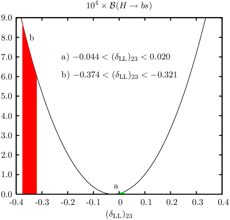
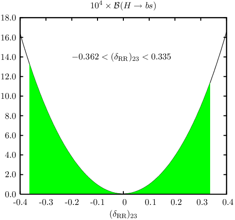
As a first step, we select one possible type of flavour violation in the squark sector, assuming that all the others vanish. The interference between different types of flavour mixing is thus ignored. We found that the flavour-off-diagonal elements are independently constrained to be at most –. As expected [121, 122, 325, 326, 327], the bounds on are the strongest, –. The data from further constrain the parameters and , the others remaining untouched. The allowed intervals for the corresponding flavour-mixing parameters thus obtained are given in [123]. For our reference point (3.78) we find that the largest allowed value of , of or , is induced by or , respectively (see Fig.3.14). These are the flavour-changing parameters least stringently constrained by the data. can reach if induced by or by , the most stringently constrained flavour-changing parameter. Because of the restrictions imposed by , depends very little on and .
Then, we investigate the case when two off-diagonal elements of the squark mass matrix contribute simultaneously. Indeed, we performed the analysis for all possible combinations of two of the four dimensionless parameters (3.77). The full results are given in [123]. Fig. 3.15 displays part of the results for our parameter set (3.78). Contours of constant are drawn for various combinations – of flavour-mixing parameters, which we shall refer to as “– planes” for short in the following. The coloured bands represent regions experimentally allowed by . The red bands are regions disfavoured by . The bounds on , the best constrained for only one non-zero flavour-off-diagonal element, are dramatically relaxed when other flavour-changing parameters contribute simultaneously. Values of are allowed. As shown in Fig. 3.15, large although fine-tuned values of and combined are not excluded by , yielding e.g. . This translates to branching ratios compatible with experimental data of . 44 4 Here we have used the total width of GeV, , for the point (3.78) in the MSSM with MFV. It also occurs for the – case. The combined effects of – lead to leading to .


3.11 Squark/gaugino production and decay
Non-minimal flavour violation (NMFV) arises in the MSSM from a possible misalignment between the rotations diagonalizing the quark and squark sectors. It is conveniently parametrized in the super-CKM basis by non-diagonal entries in the squared squark mass matrices , , and and the trilinear couplings and . Squark mixing is expected to be the largest for the second and third generations due to the large Yukawa couplings involved. In addition, stringent experimental constraints for the first generation are imposed by precise measurements of and mixing. Furthermore, direct searches of flavour violation depend on the possibility of flavour tagging, established experimentally only for heavy flavours. We therefore consider here only mixings of second- and third-generation squarks and follow the conventions of Ref. [116].
3.11.1 Flavour-violating squark- and gaugino-production at the LHC
We impose mSUGRA [, , , , and sgn] parameters at a large (grand unification) scale and use two-loop renormalization group equations and one-loop finite corrections as implemented in the computer program SPheno 2.2.2 [338] to evolve them down to the electroweak scale. At this point, we generalize the squark mass matrices by including non-diagonal terms . The scaling of these terms with the SUSY-breaking scale implies a hierarchy [339]. We therefore take , while and , and assume for simplicity . The squark mass matrices are then diagonalized, and constraints from low-energy and electroweak precision measurements are imposed on the corresponding theoretical observables, calculated with the computer program FeynHiggs 2.5.1 [333].
Flavour-changing neutral-current (FCNC) -decays and mixing arise in the SM only at the one-loop level. These processes are therefore particularly sensitive to non-SM contributions entering at the same order in perturbation theory and have been intensely studied at -factories. The most stringent constraints on SUSY-loop contributions in minimal and non-minimal flavour violation come today from the inclusive decay rate as measured by BaBar, Belle, and CLEO, [340], which affects directly the allowed squark mixing between the second and third generation [123].
Another important consequence of NMFV in the MSSM is the generation of large splittings between squark-mass eigenvalues. The splitting within isospin doublets influences the - and -boson self-energies at zero-momentum in the electroweak -parameter and consequently the -boson mass and the squared sine of the weak mixing angle . The latest combined fits of the -boson mass, width, pole asymmetry, -boson and top-quark mass constrain new physics contributions to to or [340].
A third observable sensitive to SUSY loop-contributions is the anomalous magnetic moment of the muon, for which recent BNL data and the SM prediction disagree by [340]. In our calculation, we take into account the SM and MSSM contributions up to two loops [341, 342].
For cosmological reasons, we require the lightest SUSY particle (LSP) to be electrically neutral. We also calculate, albeit for minimal flavour violation () only, the cold dark matter relic density using the computer program DarkSUSY [343] and impose a limit of at 95% (2) confidence level. This limit has recently been obtained from the three-year data of the WMAP satellite, combined with the SDSS and SNLS survey and Baryon Acoustic Oscillation data and interpreted within a more general (11-parameter) inflationary model [344]. This range is well compatible with the older, independently obtained range of [281].
Typical scans of the mSUGRA parameter space with , and and all experimental limits imposed at the level are shown in Fig. 3.16. Note that is disfavored by


data, while only constrains the parameter space outside the mass regions shown here. In minimal flavour-violation, light SUSY scenarios such as the SPS 1a benchmark point ( GeV, GeV) [244] are favored data. The dependence on the trilinear coupling ( GeV for SPS 1a, GeV in our scenario) is extremely weak.
In Fig. 3.17 we show for our (slightly modified) SPS 1a


benchmark point the dependence of the electroweak precision variables and the lightest SUSY particle masses on the NMFV parameter , indicating by dashed lines the ranges allowed experimentally within two standard deviations. It is interesting to see that for this benchmark point, not only the region close to minimal flavour violation () is allowed, but that there is a second allowed region at .
Next, we study in Fig. 3.18 the chirality and flavour

decomposition of the light (1,2) and heavy (4,6) squarks, which changes mostly in a smooth way, but sometimes dramatically in very small intervals of . In particular, the second allowed region at larger has a quite different flavour and chirality mixture than the one at small .
The main result of our work is the calculation of all electroweak (and strong) squark and gaugino production channels in NMFV SUSY [345]. We show in Fig. 3.19 a small, but representative sample of


these production cross sections: charged squark-antisquark pair production, non-diagonal squark-squark pair production, as well as chargino-squark and neutralino-squark associated production. The two allowed regions ( and ) are indicated by vertical lines. Note that NMFV allows for a top-flavour content to be produced from non-top initial quark densities and for right-handed chirality content to be produced from strong gluon or gluino exchanges. The cross sections shown here are all in the fb range and lead mostly to experimentally identifiable heavy-quark (plus missing transverse-energy) final states.
In conclusion, we have performed a search in the NMFV-extended mSUGRA parameter space for regions allowed by electroweak precision data as well as cosmological constraints. In a benchmark scenario similar to SPS 1a, we find two allowed regions for second- and third-generation squark mixing, and , with distinct flavour and chirality content of the lightest and heaviest up- and down-type squarks. Our calculations of NMFV production cross sections at the LHC demonstrate that the corresponding squark (anti-)squark pair production channels and the associated production of squarks and gauginos are very sensitive to the NMFV parameter . For further details see Ref. [346].
3.11.2 Flavour-violating squark and gluino decays
In the study of squark decays two general scenarios can be distinguished depending on the hierarchy within the SUSY spectrum:
- •
(; ): In this case the gluino will mainly decay according to
(3.79) with and followed by squark decays into neutralino and charginos
(3.80) In addition there can be decays into gauge- and Higgs bosons if kinematically allowed:
(3.81) (3.82) where , , . Due to the fact, that there is left-right mixing in the sfermion mixing, one has flavour changing neutral decays into -bosons at tree-level.
- •
(; ): In this case the squarks decay mainly into a gluino:
(3.83) and the gluino decays via three-body decays and loop-induced two-body decays into charginos and neutralinos
(3.84) with , and . The first two decay modes contain states with quarks of different generations.
Obviously, the flavour mixing final states of the decays listed above are constrained by the fact that all observed phenomena in rare meson decays are consistent with the SM predictions. Nevertheless, one has to check how large the branching ratios for the flavour mixing final states still can be. One also has to study the impact of such final states on discovery of SUSY as well as the determination of the underlying model parameters.
For simplicity we restrict ourselves to the mixing between second and third generation of (s)quarks. We will take the so–called SPA point SPS1a’ [255] as a specific example which is specified by the mSUGRA parameters GeV, GeV, GeV, and . We have checked that main features discussed below are also present in other study points, e.g. and of [347]. At the electroweak scale (1 TeV) one gets the following data with the SPA1a’ point: GeV, GeV, GeV and GeV. We have used the program SPheno [338] for the calculation.
It has been shown, that in Minimal Flavour Violating scenarios the flavour changing decay modes are quite small [196]. To get sizable flavour changing decay branching ratios, we have added the flavour mixing parameters as given in Table 3.7; the resulting up-squark masses in GeV are in ascending order: 315, 488, 505, 506, 523 and 587 [GeV] whereas the resulting down-squark masses are 457, 478, 505, 518, 529, 537 [GeV]. This point is a random, but also typical one out of 20000 points fulfilling the constraints derived from the experimental measurements of the following three key observables of the sector: , and . For the calculation we have used the formula given in [348, 349], for , the formula for given in [350] and the formula for given in [348, 351]. Note, that we have included all contributions mediated by chargino, neutralino and gluino loops as we depart here considerably from Minimal Flavour Violation. The most important branching ratios for gluino and squark decays are given in Table 3.8. In addition the following branching ratios are larger than 1%, namely BR()=8.9% and BR()=1.8%. We have not displayed the branching ratios of the first generation nor the ones of the gluino into first generation.
| -18429 | -37154 | -32906 | 28104 | 16846 | 981 | -853 |
|---|
| 1.4 | 16.8 | 81.1 | |||||||
| 9.1 | 21.0 | 3.6 | 42.9 | 14.3 | 5.3 | 1.3 | |||
| 20.9 | 21.9 | 47.5 | 1.1 | 1.9 | 5.5 | ||||
| 1.5 | 2.7 | 1.6 | 3.7 | 4.0 | 14.1 | 14.2 | 39.2 | 5.2 | |
| 1.4 | 5.7 | 2.7 | 2.8 | 6.5 | 28.1 | 27.3 | |||
| 4.2 | 2.9 | 6.3 | 17.8 | 13.4 | 18.8 | 34.8 | |||
| 1.8 | 23 | 3.7 | 41.5 | 5.8 | 20.0 | ||||
| 77.3 | 15.9 | 4.6 | 3.7 | 2.4 | 2.4 | 7.7 | 5.1 | 40. | |
| 3.4 | 12.8 | 5.5 | 7.5 | 8.2 | 5.8 | 5.1 | 2.1 | 2.2 | |
| 1.2 | 14 | 8.8 | 7.9 | 8.2 | 5.5 |
It is clear from Table 3.8 that all listed particles have large flavour changing decay modes. This clearly has an impact on the discovery strategy of squarks and gluinos as well as on the measurement of the underlying parameters. For example, in mSUGRA points without flavour mixing one finds usually that the left-squarks of the first two generations as well as the right squarks have similar masses. Large flavour mixing implies that there is a considerable mass splitting as can be seen by the numbers above. Therefore, the assumption of nearly equal masses should be reconsidered if sizable flavour changing decays are discovered in squark and gluino decays.
An important part of the decay chains considered for SPS1a’ and nearby points are which are used to determine the gluino mass as well as the sbottom masses or at least their average value if these masses are close. In the analysis the existence of two b-jets has been assumed, which need not to be the case as shown in the example above. Therefore, this class of analysis should be re-done requiring only one b-jet + one additional non b-jet to study the impact of flavour mixing on the determination of these masses.
Similar conclusions hold for the variable defined in [352]. For this variable one considers final states containing . In our example, three u-type squarks contribute with branching ratios larger than 10% in contrast to assumption that only the two stops contribute. The influence of the additional state requires for a sure a detailed Monte Carlo study which should be carried out in the future.
3.12 Top squark production and decay
Supersymmetric scenarios with a particularly light stop have been recently considered as potential candidates to provide a solid explanation of the observed baryon asymmetry of the Universe [353]. Independently of this proposal, measurements of the process of stop-chargino associated production at LHC have been considered as a rather original way of testing the usual assumptions about the Supersymmetric CKM matrix [354]. In a very recent paper [355], the latter associated production process has been studied in some detail for different choices of the SUSY benchmark points, trying to evidentiate and to understand an apparently strong dependence of the production rates. As a general feature of that study, the values of the various rates appeared, typically, below the one size, to be compared with the (much) bigger rates of the stop-antistop process (see e.g. [356]).
3.12.1 Associated stop-chargino production at LHC: A light stop scenario test
Given the possible relevance of an experimental determination, it might be opportune to perform a more detailed study of the production rate size in the special light stop scenario, where one expects that the numerical value is as large as possible. Here we present the results of this study, performed at the simplest Born level given the preliminary nature of the investigation.
The starting point is the expression of the differential cross section, estimated at Born level in the c.m. frame of the incoming pair of the partonic process . Its detailed expression has been derived and discussed in [355]. The associated c.m. energy distribution (at this Born level identical to the final invariant mass distribution) is
| (3.85) |
where and are the parton and total c.m. energies, respectively, , and is the parton process luminosity that we have evaluated using the parton distribution functions from the Heavy quark CTEQ6 set [357]. The rapidity and angular integrations are performed after imposing a cut GeV.
For a preliminary analysis, we have considered the total cross section (for producing the lightest stop-chargino pair), defined as the integration of the distribution from threshold to a final energy left as free variable, generally fixed by experimental considerations. To have a first feeling of the size of this quantity, we have first estimated it for two pairs of sensible MSSM benchmark points. The first pair are the ATLAS Data Challenge-2 points SU1, SU6 whose detailed description can be found in [137]. The second pair are the points LS1, LS2 introduced in [136]. These points are typical light SUSY scenarios and in particular share a rather small threshold energy which appears to be a critical parameter for the observability of the considered process. The main difference between SU1 and SU6 or LS1 and LS2 is the value of (larger in SU6 and LS2). The results are shown in Fig. 3.20. As one sees, the various rates are essentially below the one size, well below the expected stop-antistop values.
In the previous points, no special assumptions about the value of the stop mass were performed, hence keeping a conservative attitude. One sees, as expected, that the bigger rate values correspond to the lighter stop situations (LS1 and LS2). In this spirit, we have therefore considered a different MSSM point where the final stop is particularly light. More precisely, we have concentrated our analysis on the point LST2, introduced and discussed in Section 3.12.2 and characterized by the MSSM parameters (we list the relevant ones at Born level)
| (3.86) |
and consistent with the cosmological experimental bounds on the relic density. Now the threshold energy is even smaller than in the previous examples. The integrated cross section, shown in Fig. 3.21 reaches a maximum of about 2 pb, that might be detected by a dedicated experimental search.
3.12.2 Exploiting gluino-to-stop decays in the light stop scenario
To achieve a strong first-order electroweak phase transition in the MSSM, the lighter of the two stops, , has to be lighter than the top quark [358, 359, 360, 361, 362]. Assuming a stable LSP, there hence exists a very interesting parameter region with a small – mass difference, for which (i) coannihilation with [363, 364] leads to a viable neutralino relic density and (ii) the light stop decays dominantly into [365].
In this case, stop-pair production leads to 2 -jets , a signal which is of very limited use at the LHC. One can, however, exploit [366] gluino-pair production followed by gluino decays into stops and tops: since gluinos are Majorana particles, they can decay either into or ; pair-produced gluinos therefore give same-sign top quarks in half of the gluino-to-stop decays. Here note that in the light stop scenario, (or ) has practically 100% branching ratio. With , , and the ’s decaying leptonically, this leads to a signature of two -jets plus two same-sign leptons plus jets plus missing transverse energy:
| (3.87) |
In [366] we performed a case study for the ‘LST1’ parameter point with GeV, GeV, GeV and showed that the signature Eq. (3.87) is easily extracted from the background. In this contribution, we focus more on the stop coannihilation region and discuss some additional issues.
We define a benchmark point ‘LST2’ in the stop coannihilation region by taking the parameters of LST1 and lowering the stop mass to GeV. We generate signal and background events equivalent to of integrated luminosity and perform a fast simulation of a generic LHC detector as described in [366]. The following cuts are then applied to extract the signature of Eq. (3.87):
- •
require two same-sign leptons ( or ) with GeV;
- •
require two -tagged jets with GeV;
- •
missing transverse energy GeV;
- •
demand two combinations of the two hardest leptons and -jets
that give invariant masses GeV, consistent with a top quark.
This set of cuts emphasizes the role of the same-sign top quarks in our method, and ignores the detectability of the jets initiated by the decay. Table 3.9 shows the effect of the cuts on both the signal and the backgrounds. Detecting in addition the (soft) -jets from the decay, together with the exess in events with 2 -jets from stop-pair production, can be used to strengthen the light stop hypothesis. A reasonable -tagging efficiency would be very helpful in this case.
| Cut | 2lep, 2 | 2 | SS | ||
|---|---|---|---|---|---|
| Signal: | 1091 | 949 | 831 | 413 | |
| Background: | SM | 34224 | 8558 | 8164 | 53 |
| SUSY | 255 | 209 | 174 | 85 |


To demonstrate the robustness of the signal, we show in Fig. 3.22 (left) contours of , and significance55 5 We define significance as , where and are the numbers of signal and background events. in the (, ) plane. For comparison we also show as a dotted line the result of a CMS study [3], which found a reach down to pb in terms of the total cross section for same-sign top production. In Fig. 3.22 (right), we show the decreasing significance for GeV, as the stop–neutralino mass difference goes to zero. To be conservative, both panels in Fig. 3.22 assume that all squarks other than the are beyond the reach of the LHC; and production would increase the signal through decays (provided ) while adding only little to the background; see [366, 367] for more detail.
The usual way to determine SUSY masses in cascade decays is through kinematic endpoints of the invariant-mass distributions of the SM decay products, see e.g. [368, 253, 254, 369]. In our case, there are four possible endpoints: , , and , of which the first simply gives a relationship between the masses of the and the top, and the second and third are linearly dependent, so that we are left with three unknown masses and only two equations. Moreover, because of the information lost with the escaping neutrino the distributions of interest all fall very gradually to zero.
In order to nevertheless get some information on the , and masses, we fit the whole and distributions [366, 370] and not just the endpoints. This requires, of course, the detection of the jets stemming from the decay. For small these are soft, so we demand two jets with GeV in addition to the cuts listed above. The results of the fits for LST2, assuming 20% -tagging efficiency, 66 6 When one or none of the remaining jets are -tagged we pick the -jets as the hardest jets with GeV. are shown in Fig. 3.23. The combined result of the two distributions is , as compared to the nominal value of GeV.

As mentioned above, the gluino-pair production leads to 50% same-sign (SS) and 50% opposite-sign (OS) top-quark pairs, and hence with denoting the number of events. In contrast, in the SM one has . This offers a potential test of the Majorana nature of the gluino. The difficulty is that the number of OS leptons is completely dominated by the background. This can easily be seen from the last two rows of Table 3.9: (0.02) for the signal (backgrounds) as expected; signal and backgrounds combined, however, give . A subtraction of the background as described in Section 3.12.3 may help to extract .
3.12.3 A study on the detection of a light stop squark with the ATLAS detector at the LHC
We present here an exploratory study of a benchmark model in which the stop quark has a mass of 137 GeV, and the two-body decay of the stop squark into a chargino and a quark is open. We address in detail the ability of the ATLAS experiment to separate the stop signal from the dominant Standard Model backgrounds.
For the model under study[166] all the masses of the first two generation squarks and sleptons are set at 10 TeV, and the gaugino masses are related by the usual gaugino mass relation . The remaining parameters are thus defined:
The resulting relevant masses are GeV, GeV, 58 GeV. The decays with 100% BR into , and decays with 100% BR into an off-shell and . The final state signature is therefore similar to the one for production: 2 -jets, and either 2 leptons () (4.8% BR) or 1 lepton and 2 light jets (29% BR).
The signal cross-section, calculated at
NLO with the PROSPINO[356] program is 412 pb.
We analyze here the semi-leptonic channel, where only one of the two
legs has a lepton in the final state.
We apply the standard cuts for the search of the semileptonic top
channel as applied in [1], but with softer requirements
on the kinematics:
- •
One and only one isolated lepton (, ), GeV.
- •
GeV.
- •
At least four jets GeV, GeV.
- •
Exactly two jets in the events must be tagged as -jets, anda congratulacin they both must have GeV. The standard ATLAS b-tagging efficiency of 60% for a rejection factor of 100 on light jets is assumed.
A total of 600k SUSY events were generated using HERWIG 6.5
[307, 371],
1.2M events using PYTHIA 6.2[372].
The only additional background considered for this exploratory
study was the associated production of a W boson with two jets
and two non- jets, with the W decaying into or .
This is the dominant background for top
searches at the LHC. For this process, we generated
60k events using Alpgen[308].
The number of events generated corresponds to fb-1.
The generated events are then passed through ATLFAST,
a parametrized simulation of the ATLAS detector [45].
After the selection cuts the efficiency for the background is
3.3%77
7
The emission of additional hard jets at higher
orders in the QCD interaction can increase the probability that
the events satisfy the requirement of 4 jets. The
cut efficiency is observed to increase by about 20% if MC@NLO is
used to generate the background. We do not expect such an effect
to change the conclusions of the present analysis, but future studies should
take it into account.,
for 3.1%, and for the signal 0.47%, yielding a background
which is 15 times higher than the signal.
An improvement of the signal/background ratio can be obtained using the minimum invariant mass of all the non-b jets with GeV. This distribution peaks near the value of the W mass for the top background, whereas the invariant mass for the signal should be smaller than 54 GeV, which is the mass difference between the and the . Requiring GeV improves the signal/background ratio to 1/10, with a loss of a bit more than half the signal. We show in the left plot of Figure 3.24 after this cut the distributions for the variable , i.e. the invariant mass for the combination a b-tagged jet and the two non-b jets yielding the minimum invariant mass. If the selected jets are from the decay of the stop, this invariant mass should have an end point at 79 GeV, whereas the corresponding end-point should be at 175 GeV for the top background. The presence of the stop signal is therefore visible as a shoulder in the distribution as compared to the pure top contribution. A significant contribution from is present, without a particular structure.


Likewise, the variable has an end point at 66 GeV for the signal and at 175 GeV for the top background, as shown in Figure 3.24, and the same shoulder structure is observable. We need therefore to predict precisely the shape of the distributions for the top background in order to subtract it from the experimental distributions and extract the signal distributions.
The top background distributions can be estimated from the data themselves by exploiting the fact that we select events where one of the from the top decays into two jets and the other decays into lepton neutrino. One can therefore select two pure top samples, with minimal contribution from non-top events by applying separately hard cuts on each of the two legs.
- •
Top sample 1: the best reconstructed invariant mass is within 15 GeV of 175 GeV, and GeV in order to minimize the contribution from the stop signal. The neutrino longitudinal momentum is calculated by applying the mass constraint.
- •
Top sample 2: the best reconstructed mass is within 10 GeV of 175 GeV.
We assume here that we will be able to predict the background through a combination of Monte Carlo and the study of production in the data, and we subtract this background both from the observed distributions and from the Top samples. More work is required to assess the uncertainty on this subtraction. Given the fact that this background is smaller than the signal, and it has a significantly different kinematic distribution, we expect that a 10-20% uncertainty on it will not affect the conclusions of the present analysis.
For Top sample 1, the top selection is performed by applying severe cuts on the lepton leg, it can therefore be expected that the minimum invariant mass distribution, which is built from jets from the decay of the hadronic side be essentially unaffected by the top selection cuts. This has indeed be verified to be the case [166]. The distribution from Top sample 1 is then normalized to the observed distribution in the high mass region, where no signal is expected, and subtracted from it. A similar procedure is followed for the distribution: the top background is estimated using Top sample 2, normalized to the observed distribution in the high-mass region, and subtracted from it.


The results are shown in Figure 3.25, with superimposed the corresponding distributions for the signal. As discussed above, we have subtracted the background from the observed distributions.
For both variables the true and measured distributions for the signal are compatible, showing the goodness of the background subtraction technique, and the expected kinematic structure is observable, even with the very small statistics generated for this analysis, corresponding to little more than one month of data taking at the initial luminosity of cm-1s-1.
Further work, outside the scope of this initial exploration, is needed on the evaluation of the masses of the involved sparticles through kinematic studies of the selected sample
A preliminary detailed analysis of a SUSY model with a stop squark lighter than the top quark decaying into a chargino and a -jet was performed. It was shown that for this specific model after simple kinematic cuts a signal/background ratio of 1/10 can be achieved. A new method, based on the selection of pure top samples to subtract the top background was demonstrated. Through this method it is possible to observe the kinematic structure of the stop decays, and thence to extract a measurement of the model parameters. This analysis can yield a clear signal for physics beyond the SM for just fb-1, and is therefore an excellent candidate for early discovery at the LHC.
3.12.4 Stop decay into right-handed sneutrino LSP
Right-handed neutrinos offer the possibility to accommodate neutrino masses. In supersymmetric models this implies the existence of right-handed sneutrinos. Right-handed sneutrinos are expected to be as light as other supersymmetric particles [373, 374] if the neutrinos are either Dirac fermions or if the lepton-number breaking scale is at (or below) the SUSY breaking scale , assumed to be around the electroweak scale. Depending on the mechanism of SUSY breaking, the lightest right-handed sneutrino may be the lightest supersymmetric particle (LSP). We consider in the following such a scenario focusing on the case where the right-handed stop is the next to lightest SUSY particle assuming -parity conservation. Details on the model and other scenarios can be found in [373, 374].
As the right-handed neutrino has a mass around 100 GeV, the neutrino Yukawa couplings must be very small to accommodate neutrino data: () in the case of Majorana neutrinos (Dirac neutrinos). This has as immediate consequence that if the SUSY breaking sneutrino trilinear “A-term” is also proportional to , the left-handed and right-handed sneutrinos hardly mix independent of neutrino physics because the left-right mixing term is proportional to . Decays into will give tiny decay widths as is the only coupling of . For this reason, all decays of supersymmetric particles are as in the usual MSSM, but for the NLSP whose life-time can be long since it can only decay into the . In the case of a stop NLSP the dominant decay mode is , followed by CKM suppressed ones into and quarks. In the limit where mixing effects for stops and charginos are neglected the corresponding matrix element squared in the rest frame of the stop reads as:
| (3.88) |
where we have assumed that the right-handed stop is the lightest stop and is the Higgsino, () is the energy of the b-quark (lepton), is the angle between the fermions. The complete formula can be found in [374]. The last factor in Eq. (3.88) implies that the -quark and the lepton have a tendency to go in the same direction.
In the following we summarize the results of a Monte Carlo study at the parton level [374] using PYTHIA 6.327 [375]. We have taken 225 GeV, 100 GeV, 250 GeV and resulting in a mean decay length of 10 mm. Note, that the stop will hadronize before decaying. However, we have neglected the related effects in this study. We have only considered direct stop pair production, and neglected stops from cascade decays, e.g. . The signal is . The dominant physics background is top quark pair production: , where the missing energy is due to neutrinos in the final state. We have imposed the following ”Level 1” cuts: (i) fermion rapidities: , (ii) cuts GeV, GeV and (iii) isolation cut .
Figure 3.26 shows various distributions for stop and top decays. Figure 3.26a) depicts the resulting transverse displacement after including the boost of the stop. If it decays before exiting the tracking subsystem, a displaced vertex may be reconstructed through the stop decay products’ 3-momenta meeting away from the primary interaction point. On each side, the -quark itself leads to an additional displaced vertex, and its 3-momentum vector can be reconstructed from its decay products. In combination with the 3-momentum of the lepton, the stop displaced vertex can be determined. In order to reveal the displaced vertex, one must require either the -quark or the charged lepton 3-momentum vector to miss the primary vertex. Since a pair of stops is produced, we would expect to discern two displaced vertices in the event (not counting the displaced vertices due to the b-quarks). Such an event with two displaced vertices, from each of which originates a high and -quark might prove to be the main distinguishing characteristics of such a scenario. A cut on the displaced vertex will be very effective to separate stop events from the top background provided one can efficiently explore such cuts. We anticipate that NLSP stop searches may turn out to be physics-background free in such a case.
If the stop displaced vertex cannot be efficiently resolved, one will have to resort to more conventional analysis methods. In the remainder we explore various kinematical distributions for both the signal ( pair production) and the physics background ( pair production), obtained after imposing the level 1 cuts given above. Figures 3.26b) and c) depict the spectra of the produced fermions. The of the -quark from the GeV stop peaks at a lower value compared to the top quark background, and therefore accepting them at high efficiency for GeV will be very helpful in maximizing the signal acceptance. The signal and background shapes are quite similar and no simple set of cuts can be made in order to significantly separate signal from background.
Fig. 3.26d) depicts the distribution of , the angle between the 3-momenta and , for both the signal and background. It is important to appreciate that, by default, PYTHIA generates stop decays into the 3-body final state according only to phase-space, ignoring the angular dependence of the decay matrix element. We have reweighted PYTHIA events to include the correct angular dependence in the decay matrix element. Consistent with the expectation from Eq. (3.88), we see for the signal that the distribution peaks for the -quark and charged lepton 3-momenta aligned, unlike the background. It is unfortunate that the isolation level 1 cut on the leptons removes more signal events than background events. Relaxing this constraint as much as practical would help in this regard. Additional work will be necessary to include also the effect of spin correlations in top production and top decays so that information from the quantities and can be exploited.
Assuming efficiencies of and for -quark and lepton identification, respectively, it has been shown in [374] that stops with masses up to 500 GeV can be detected at the 5 level for an integrated luminosity of 10 fb-1 if even if the displaced vertex signature is not used. Clearly, the situation will be worse in the case of . Provided one can exploit the displaced vertex information, we expect a considerable improvement as we could not identify any physics background. Further studies are planned to investigate the questions we have touched upon here.
3.13 SUSY Searches at TeV with CMS
This section summarizes the recent results on SUSY searches reported at [57]. In the context of this work we refer to the generalized classification of models of new physics according to how they affect flavour physics:
- •
CMFV: Constrained Minimal Flavour Violation [376] models: in these models the only source of quark flavour violation is the CKM matrix. Examples include minimal supergravity models with low or moderate tan, and models with a universal large extra dimension.
- •
MFV: Minimal Flavour Violation [195] models: a set of CMFV models with some new relevant operators that contribute to flavour transitions. Examples include SUSY models with large tan.
- •
NMFV: Next-to-Minimal Flavour Violation [377] models: they involve third generation quarks and help to solve the flavour problems that appear in frameworks such as Little Higgs, topcolour, and RS models.
- •
GFV: General Flavour Violation [378] models; they provide with new sources of flavour violation. These include most of the MSSM parameter space, and almost any BSM model before flavour constraints are considered.
A useful discussion on these models can be found in [379]. The SUSY searches that are summarized here fall in the category of MFV (mSUGRA specifically) and all results are obtained with the detailed Geant-4 based CMS simulation. In the context of this workshop and in collaboration with the theory community we try to also move towards interpretation within NMVF models (see e.g contributions by R. Cavanaugh and O. Buchmueller in this volume). Note that since the squarks and sleptons can have significant flavour changing vertices and be complex, the connection to collider physics can be subtle indeed, the main implication being that the superpartners cannot be too heavy and that larger tan is favored – with no direct signature in general. For interpretations of recent Tevatron and B-factory results the interested reader can refer for example to [380], [381], [382], [383] and to relevant contributions at this workshop.
The SUSY search path has been described in the past years as a successive approximation of serial steps that move from inclusive to more exclusive measurements as follows:
- •
Discovery: using canonical inclusive searches
- •
Characterization: putting together a picture given the channels that show excess and ratios of the observed objects (e.g. multi-leptons, photons (GMSB), ratio of same sign leptons to opposite ones, ratios of positive pairs to negative, departure from lepton universality, third generation excesses).
- •
Reconstruction: in canonical dark matter LSP SUSY the final state contains two neutralinos hence there is no direct mass peak due to the missing transverse energy in the event. The kinematics of the intermediate decays provide however a multitude of endpoints and edges that might provide mass differences and help orient towards the right mass hierarchy.
- •
Measurement of the underlying theory: the classical SUSY solving strategy involves more mass combinations, more decay chains, mass peaks and once the LSP mass is known the determination of the mass hierarchies, particles’ spins, and eventually the model parameters. An outstanding question remains as to how many simple measurements do we need to “nail” the theory? Remember that we did not need to measure all the Standard Model particles and their properties in order to measure the Standard Model.
In the past three years the “inclusive” and “exclusive” modus quaestio questio have been approached in coincidence and in many works that range in exploitation strategy from statistical methods to fully on-shell description of unknown models and inclusion of cosmological considerations such as in [384], [385], [386], [247] and [387], to mention but a few.
It is rather safe to claim that the program of discovery and characterization will be (much) more convoluted than the one described in the serial steps above. Realistic studies of kinematic edges across even the “simple” mSUGRA parameter space show that this is a difficult job and it will take a lot of work and wisdom to do it right. Endpoint analyses by definition involve particles which are very soft in some reference frame and non trivial issues of acceptance need to be considered.
Some of most recent SUSY searches at CMS [57], proceed in the following channels:
- •
canonical inclusive
- –
multijets+
- –
+jets+
- –
same-sign dimuon +
- –
opposite-sign same flavour dielectron and dimuon +
- –
opposite-sign same flavour hadronic ditau +
- –
trileptons at high
- –
- •
higher reconstructed object inclusive
- –
+
- –
hadronic top +
- –
+
- –
- •
flavour violating
- –
opposite-sign different flavour FV neutralino decays (contributing to this workshop also)
- –
The attempt is to have an as model-independent signature-based search strategy with educated input from theory. The interpretation of the search results are given in the context and parameter space of mSUGRA but re-interpreting them in different models is possible. All of the searches are including detector systematic uncertainties and a scan that provides the 5 reach in the mSUGRA parameter space is derived for 1 and 10 as shown in figure 3.27


The details of the analyses and individual search results can be found at [57].
Chapter 4 Non-supersymmetric Standard Model extensions
J. A. Aguilar Saavedra and G. Ünel
4.1 Introduction
Although the Standard Model (SM) has seemingly survived many stringent tests offered by both precision measurements and direct searches, it has a number of shortcomings. The most unpleasant one is the “instability” of the Higgs boson mass with respect to radiative corrections, known as the hierarchy problem. If the SM is assumed valid up to a high scale of the order of the Planck mass, radiative corrections to from top quark loops are of order , i.e. much larger than which is expected to be of the order of the electroweak scale. The requirement that and are of the same order would imply a cutoff (and hence new physics at) TeV. Some other aspects of the SM that make it unappealing as the ultimate theory of fundamental interactions (excluding gravity) are:
- •
the lack of simplicity of the gauge structure,
- •
the large hierarchy of fermion masses and quark mixings, and the large number of apparently free parameters necessary to describe them,
- •
the source of baryogenesis, which can not be explained by the amount of CP violation present in the SM,
- •
the unknown mechanism behind the neutrino mass generation (neutrinos can have Dirac masses simply with the introduction of right-handed fields, but present limits eV require unnaturally small Yukawa couplings).
Therefore, the SM is believed to be the low-energy limit of a more fundamental theory. Several arguments suggest that this theory may manifest itself at energies not much higher than the electroweak scale, and give support to the hope that LHC will provide signals of new physics beyond the SM.
This chapter deals with non-supersymmetric candidate theories as extensions to the SM. Among the most frequently studied ones, the following ones can be mentioned.
- 1.
Grand unified theories (GUTs). In these models the SM gauge group is embedded into a larger symmetry group, which is recovered at a higher scale. They predict the existence of new fermions (e.g. singlets) and new gauge bosons (especially ), which may be at the reach of LHC.
- 2.
Little Higgs models. They address the hierarchy problem with the introduction of extra gauge symmetries and extra matter which stabilise the Higgs mass up to a higher scale TeV. In particular, the top quark loop contribution to the Higgs mass is partially cancelled with the introduction of a quark singlet .
- 3.
Theories with extra dimensions. The various extra-dimensional models avoid the hierarchy problem by lowering the Planck scale in the higher dimensional theory, and some of them can explain the large hierarchies between fermion masses. The observable effect of the additional dimension is the appearance of “towers” of Kaluza-Klein (KK) excitations of fermions and bosons, with increasing masses. Depending on the model, the lightest modes can have a mass around the TeV scale and thus be produced at LHC.
It should be stressed that these SM extensions, sometimes labelled as “alternative theories” do not exclude supersymmetry (SUSY). In fact, SUSY in its minimal versions does not address some of the open questions of the SM. One example is the motivation behind the apparent gauge coupling unification. The renormalisation-group evolution of the coupling constants strongly suggests that they unify at a very high scale GeV, and that the SM gauge group is a subgroup of a larger one, e.g. , or other possibilities. Thus, SUSY can naturally coexist with GUTs. Another example of complementarity is SUSY + Little Higgs models. If SUSY is broken at the TeV scale or below, it may give dangerous contributions to flavour-changing neutral (FCN) processes and electric dipole moments (EDMs). These contributions must be suppressed with some (well justified or not) assumption, like minimal supergravity (MSUGRA) with real parameters. These problems are alleviated if SUSY is broken at a higher scale and, up to that scale, the Higgs mass is stabilised by another mechanism, as it happens in the Little Higgs theories.
With the forthcoming LHC, theories beyond the SM will be tested directly through the searches of the new particles, and indirectly, with measurements of the deviations from SM precision variables. Instead of studying the different SM extensions and their additional spectrum separately, we follow a phenomenological/experimental approach. Thus, this chapter is organised according to the new particles which are expected to be produced. Section 4.2 reviews the searches for the new quarks and section 4.3 for new heavy neutrinos. Studies for new gauge bosons are collected in sections 4.4 and 4.5, and in section 4.6 some new scalar signals are presented. Detailed information about the SM extensions predicting these new particles is not included in this report for brevity (although the text is as self-contained as possible). Instead, the interested reader is encouraged to refer to the original papers and dedicated reviews (see for instance [388, 389, 390, 391, 392]). The observation of these new particles would prove, or at least provide hints, for the proposed theories. In this case, the identification of the underlying theory might be possible with the measurement of the couplings, production and decay modes of the new particle(s). Alternatively, the non-observation of the predicted signals would disprove the models or impose lower bounds for their mass scales.
4.2 New quarks
At present, additional quarks are not required neither by experimental data nor by the consistency of the SM. But on the other hand they often appear in Grand Unified Theories [59, 393], Little Higgs models [394, 395, 390], Flavour Democracy[396] and models with extra dimensions [397, 24, 392]. Their existence is not experimentally excluded but their mixing, mainly with the lightest SM fermions, is rather constrained. They can lead to various indirect effects at low energies, and their presence could explain experimental deviations eventually found, for instance in asymmetries in decays. They can also enhance flavour-changing processes, especially those involving the top quark. These issues have been dealt with in other chapters of this report. Here we are mainly concerned with their direct production and detection at LHC.
New quarks share the same electromagnetic and strong interactions of standard quarks, and thus they can be produced at LHC by annihilation and gluon fusion in the same way as the top quark, with a cross section which only depends on their mass, plotted in Fig. 4.1. Depending on their electroweak mixing with the SM fermions, they can be produced singly as well [398, 399, 400]. Their decay always takes place through electroweak interactions or interactions with scalars, and the specific decay modes available depend on the particular SM extension considered. Let us consider a SM extension with “standard” chiral generations (left-handed doublets and right-handed singlets under ), plus up-type and down-type singlets under this group.11 1 Anomaly cancellation requires that the number of lepton generations is also . For this implies additional neutrinos heavier than to agree with the invisible width measurement at LEP. On the other hand, quark singlets can be introduced alone, since they do not contribute to anomalies [393]. While (left-handed) doublets couple to the and bosons, singlet fields do not. The Lagrangian in the weak eigenstate basis reads
| (4.1) | |||||
| (4.2) |
where are the doublets under and is the electromagnetic current which includes all (charged) quark fields. The number of mass eigenstates with charges and is , , respectively. The resulting weak interaction Lagrangian in the mass eigenstate basis is
| (4.3) | |||||
| (4.4) |
where , are column vectors of dimensions , , and is the electromagnetic current (including all mass eigenstates). The matrix (not necessarily square) is the generalisation of the CKM matrix. The matrices , have dimensions and , respectively. In case that the up-type mass eigenstates are mixture of weak eigenstates with different isospin, and thus the matrix is not necessarily diagonal. In other words, is not unitary (but its submatrix involving SM quarks is almost unitary), what prevents the GIM mechanism from fully operating. Analogous statements hold for the down sector. Therefore, models with quark singlets can have tree-level flavour-changing neutral (FCN) couplings to the boson. These couplings are suppressed by the mass of the new mass eigenstates, e.g. (with a new charge quark), what forbids dangerous FCN currents in the down sector but allows for observable effects in top physics.

As within the SM, its extensions with extra quarks typically have one Higgs doublet which breaks the electroweak symmetry and originates the fermion masses. The surviving scalar field couples to the chiral fields (through Yukawa couplings) but not to the weak eigenstate isosinglets. In the mass eigenstate basis, the scalar-quark interactions read
| (4.5) |
with , the diagonal mass matrices, of dimensions and . SM extensions with extra quarks usually introduce further scalar fields, e.g. in additional scalar singlets are present, but with VEVs typically much higher than the mass scale of the new quarks and small mixing with . Also, in supersymmetric versions of there are two Higgs doublets, in which case the generalisation of Eq. (4.5) involves two scalar fields and the ratio of their VEVs . However, the main phenomenological features of these models can be described with the minimal scalar sector and Lagrangian in Eq. (4.5). (Of course, this does not preclude that with appropriate but in principle less natural choices of parameters one can build models with a completely different behaviour.) In particular, from Eq. (4.5) it follows that FCN interactions with scalars have the same strength as the ones mediated by the boson, up to mass factors. Note also that Eq. (4.5) does not contradict the fact that new heavy mass eigenstates, which are mainly singlets, have small Yukawa couplings. For example, with an extra singlet the Yukawa coupling of the new mass eigenstate is proportional to (see also section 4.2.1 below).
More general extensions of the SM quark sector include right-handed fields transforming non-trivially under . The simplest of such possibilities is the presence of additional isodoublets . Their interactions are described with the right-handed analogous of the terms in Eqs. (4.4) and a generalisation of Eq. (4.5). From the point of view of collider phenomenology, their production and decay takes place through the same channels as fourth generation or singlet quarks (with additional gauge bosons there would be additional modes). However, the constraints from low energy processes are much more stringent, since mixing with a heavy isodoublet can induce right-handed charged currents among the known quarks, which are absent in the SM. An example of this kind is a interaction, which would give a large contribution to the radiative decay (see chapter 2.2.2.1).
A heavy quark of either charge can decay to a lighter quark via charged currents, or to a lighter quark of the same charge via FCN couplings if they are nonzero. The partial widths for these decays are [401]
| (4.6) |
with
| (4.7) |
a kinematical function. (The superscripts , in the FCN couplings may be dropped when they are clear from the context.) Since QCD and electroweak production processes are the same for generation and exotic quarks, their decays provide the way to distinguish them. For quark singlets the neutral current decays are possible, and kinematically allowed (see below). Moreover, for a doublet of SM quarks of the same generation one has , for . Depending on the Higgs mass, decays may be kinematically allowed as well, with a partial width for much larger than the other masses involved. Both FCN decays, absent for generation heavy quarks,22 2 For generation quarks neutral decays can take place radiatively, and can have sizeable branching ratios if tree-level charged current decays are very suppressed, see section 4.2.4 . provide clean final states in which new quark singlets could be discovered, in addition to the charged current decays present in all cases. If the new quarks mix with the SM sector through right-handed interactions with the SM gauge and Higgs bosons, the decays are the same as in Eq. (4.6) but replacing and by their right-handed analogues. If the new quarks are not too heavy, the chirality of their interactions can be determined by measuring angular or energy distributions of the decay products. For instance, in a decay the charged lepton angular distribution in rest frame (or its energy distribution in rest frame) an be used to probe the interaction (see the discussion after Eq. (4.9) below, and also chapter 2.2.2.1).
Searches at Tevatron have placed the 95% CL limits GeV [340] (in charged current decays, assuming 100% branching ratio), GeV [402] (assuming BR()=1), where is a charge quark. If a priori assumptions on decays are not made, limits can be found on the branching ratios of these two channels [403] (see also [404, 405]). In particular, it is found that for quarks with masses GeV near the LEP kinematical limit there are some windows in parameter space where could have escaped discovery. For a charge quark , the present Tevatron bound is GeV [406] in charged current decays , very close to the kinematical limit where decays are kinematically possible. The prospects for LHC are reviewed in the following.
4.2.1 Singlets: charge
A new up-type singlet is expected to couple preferrably to the third generation, due to the large mass of the top quark. The CKM matrix element is expected to be of order , although for masses at the TeV scale or below the exact relation enters into conflict with latest precision electroweak data. In particular, the most stringent constraint comes from the parameter [23]. The most recent values [340] (for arbitrary), (setting ) imply the 95% CL bounds , , respectively. The resulting limits on are plotted in Fig. 4.2, including for completeness the limit from (plus other correlated observables like , the FB asymmetries and coupling parameters) and the bound on from direct searches. The mixing values obtained from the relation are also displayed, for (continuous line) and (gray band). In this class of models the new contributions to are very small, so it is sensible to use the less restrictive bound . Even in this case, mixing angles seem too large for lighter than 1.7 TeV. Of course, the importance of the bound , and indirect bounds in general, must not be neither overemphasised nor neglected. Additional new particles present in these models also contribute to and can cancel the contribution from the new quark. But this requires fine-tuning for lower masses and/or larger mixings.

The main decays of the new quark are , , , with partial widths given by Eqs. (4.6). Their characteristic features are:
- (i)
: The decays , originate very energetic charged leptons, not only due to the large mass but also to spin effects [407]: for large the charged leptons are emitted more towards the flight direction.
- (ii)
: The leptonic decays produce a very clean final state, although with a small branching ratio.
- (iii)
Discovery potential
In pair production the largest reach is provided by the mode and subsequent semileptonic decay of the pair, plus additional contributions from other decay modes giving the same signature plus additional jets or missing energy [69, 407]
| (4.8) |
These signals are characterised by one energetic charged lepton, two jets and at least two additional jets. Their main backgrounds are top pair and single top production and plus jets. Charged leptons originating from decays are much more energetic than those from , as it has been stressed above. The charged lepton energy distribution in () rest frame reads
| (4.9) | |||||
with the helicity fractions (see chapter 2.2.2.1), which satisfy . For the top quark they are , , , while for with a mass of 1 TeV they are , , . It must be pointed out that for large , even when right-handed interactions are included; thus, the chirality of this vertex cannot be determined from these observables. The maximum and minimum energies depend on the mass of the decaying fermion, and are GeV, GeV for , and GeV, GeV for (with =1 TeV). The resulting energy distributions are presented in Fig. 4.3 (left) for the same mass of 1 TeV. The larger mean energy in the rest frame of the parent quark is reflected in a larger transverse momentum in laboratory frame, as it can be observed in Fig. 4.3 (right). For the second and third decay channels in Eq. (4.8), denoted by and respectively, the tail of the distribution is less pronounced. This is so because the charged lepton originates from only half of the times, and the rest comes from and is less energetic.
 |
 |
 |
 |
Background is suppressed by requiring large transverse momenta of the charged lepton and the jets, and with the heavy quark mass reconstruction. The reconstructed masses of the heavy quarks decaying hadronically () and semileptonically () are shown in Fig. 4.4. For the leading decay mode these distributions have a peak around the true value, taken here as 1 TeV, but for the additional signal contributions the events spread over a wide range. Thus, kinematical cuts on , , considerably reduce the extra signal contributions.
The estimated discovery limits for 300 fb-1 can be summarised in Fig. 4.5. They also include the results from (plus ) production, where the decay (or ) also gives the highest sensitivity for large masses [409]. The reach in production is independent of , but the cross section scales with , and thus the sensitivity of the latter process depends on . masses on the left of the vertical line can be seen with in production. Values of and over the solid curve can be seen in production. The latter discovery limits have been obtained by rescaling the results for TeV in Refs. [409, 410]. The 95% CL bounds from the parameter (for and arbitrary) ares represented by the dashed and dotted lines, respectively. Then, the yellow area (light grey in print) represents the parameter region where the new quark cannot be discovered with , and the orange triangle (dark gray) the parameters for which it can be discovered in single but not in pair production.

Several remarks are in order regarding these results. The limits shown for and only include the channel (with additional signal contributions giving the same final state in the former case). In both analyses the evaluation of backgrounds, e.g. , does not include higher order processes with extra hard jet radiation: , , etc. These higher order contributions may be important in the large transverse momenta region where the new quark signals are searched. Systematic uncertainties in the background are not included either, and they lower the significance with respect to the values presented here. On the other hand, additional decay channels can be included and the event selection could be refined, e.g. by a probabilistic method, so that the limits displayed in Fig. 4.5 are not expected to be significantly degraded when all of these improvements are made in the analysis.
Higgs discovery from decays
Apart from the direct observation of the new quark, another exciting possibility is to discover the Higgs boson from decays [408, 401]. Very recent results from CMS have significantly lowered the expectations for the discovery of a light Higgs boson in production, with . This decrease is due to a more careful calculation of the background, and to the inclusion of systematic uncertainties [57]. As a result, a light Higgs is impossible to see in this process, with a statistical significance of only for 30 fb-1 of luminosity and GeV. But if a new quark exists with a moderate mass, its pair production and decays
| (4.10) |
provide an additional source of Higgs bosons with a large cross section (see Fig. 4.1) and a total branching ratio close to . The final state is the same as in production with semileptonic decay: one charged lepton, four or more -tagged jets and two non-tagged jets. The main backgrounds are production with two mistags and production. The inclusion of higher order () contributions is relevant because of their increasing efficiency for larger (the probability to have two mistags grows with the jet multiplicity). The larger transverse momenta involved for larger also make higher order processes more difficult to suppress with respect to the signal. Lower order contributions () are important as well, due to pile-up. The method followed to evaluate top pair production plus jets is to calculate for with Alpgen [308] and use PYTHIA 6.4 [411] to include soft jet radiation, using the MLM matching prescription [412] to avoid double counting.
 |
 |
 |
 |
Background suppression is challenging because the higher-order backgrounds are less affected by large transverse momentum requirements. Moreover, the signal charged leptons are not so energetic, and cannot be used to discriminate signal and background as efficiently as in the previous final state. Background is suppressed with a likelihood method. Signal and background likelihood functions , can be built. using as variables several transverse momenta and invariant masse, as those shown in Fig. 4.6, as well as angles and rapidities of final state particles. (Additional details can be found in Ref. [401].) Performing cuts on these and other variables greatly improves the signal observability. For a luminosity of 30 fb-1, the statistical significances obtained for the Higgs signals in final states with four, five and six jets are [401]
| (4.11) |
including a 20% uncertainty in the background. Additional backgrounds like electroweak production, (QCD and electroweak) and plus jets are smaller but have also been included. The combined significance is , a factor of 25 larger than in production alone. Then, this process offers a good opportunity to quicky discover a light Higgs boson (approximately with 8 fb-1) in final states containing a charged lepton and four or more quarks. These figures are conservative, since additional signal processes have not been included in the signal evaluation. The decay channels in Eqs. (4.10) also provide the best discovery potential for relatively close to the electroweak scale. For GeV, as assumed here, discovery of the new quark could be possible with 7 fb-1.
4.2.2 Singlets: charge
Down-type iso-singlet quark arise in the GUT models [59]. These models postulate that the group structure of the SM, , originates from the breaking of the GUT scale down to the electroweak scale, and thus extend each SM family by the addition of one isosinglet down type quark.
Following the literature, the new quarks are denoted by letters , , and . The mixings between these and SM down type quarks is responsible for the decays of the new quarks. In this study, the intrafamily mixings of the new quarks are assumed to be dominant with respect to their inter-family mixings. In addition, as for the SM hierarchy, the quark is taken to be the lightest one. The usual CKM mixings, represented by superscript , are taken to be in the up sector for simplicity of calculation (which does not affect the results). Therefore, the Lagrangian relevant for the down type isosinglet quark, , becomes a simplification of equation set 4.4. It can explicitely be written as:
| (4.12) | |||||
The measured values of ,, constrain the and mixing angle to assuming the squared sum of row elements of the new CKM matrix equal unity (see[49] and references therein for CKM matrix related measurements). The total decay width and the contribution by neutral and charged currents were already estimated in [413]. As reported in this work, the quark decays through a boson with a branching ratio of 67% and through a boson with a branching ratio of 33%. If the Higgs boson exists, in addition to these two modes, quark might also decay via the channel which is available due to mixing. The branching ratio of this channel for the case of GeV and is calculated to be about 25%, reducing the branching ratios of the neutral and charged channels to 50% and 25%, respectively [414, 415].
The discovery potential


The discovery potential of the lightest isosinglet quark has been investigated using the pair production channel which is quasi-independent of the mixing angle . The main tree level Feynman diagrams for the pair production of quarks at LHC are gluon fusion, and annihilation. The and vertices are the same as their SM down quark counterparts. The modification to the vertex due to mixing can be neglected due to the small value of .
The Lagrangian in Eq. (4.12) was implemented into tree level event generators, CompHEP 4.3 [416] and MadGraph 2.3 [417]. The impact of uncertainties in parton distribution functions (PDFs) [131], is calculated by using different PDF sets, to be less than 10% for quark mass values from 400 to 1400 GeV. For example at GeV and , the cross section values are 450 fb (CompHEP, CTEQ6L1) and 468 fb (CompHEP, CTEQ5L) versus 449 fb (MadGraph, CTEQ6L1) and 459 fb (MadGraph, CTEQ5L) with an error of about one percent in each calculation. The largest contribution to the total cross section comes from the gluon fusion diagrams for quark masses below 1100 GeV, while for higher quark masses, contributions from -channel annihilation subprocesses becomes dominant. For these computations, are assumed to be only from the first quark family since, the contribution to the total cross section from is about 10 times smaller and the contribution from and are about 100 times smaller. The -channel diagrams mediated by and bosons, which are suppressed by the small value of (for example 0.4 fb at GeV) were also included in the signal generation. The isosinglet quarks being very heavy are expected to immediately decay into SM particles. The cleanest signal can be obtained from both s decaying via a boson. Although it has the smallest branching ratio, the 4 lepton and 2 jet final state offers the possibility of reconstructing the invariant mass of bosons and thus of both quarks. The high transverse momentum of the jets coming from the quark decays can be used to distinguish the signal events from the background.
The quarks in signal events were made to decay in CompHEP into SM particles. The final state particles for both signal and background events were fed into PYTHIA version 6.218 [43] for initial and final state radiation, as well as hadronisation using the CompHEP to PYTHIA and MadGraph to PYTHIA interfaces provided by ATHENA 9.0.3 (the ATLAS offline software framework). To incorporate the detector effects, all event samples were processed through the ATLAS fast simulation tool, ATLFAST [418], and the final analysis has been done using physics objects that it produced. The cases of 4 muons, 4 electrons and 2 electrons plus 2 muons were separately treated to get the best reconstruction efficiency. As an example, table 4.1 gives the selection efficiencies for the mixed lepton case at GeV.
| channel | ||||||
|---|---|---|---|---|---|---|
| cut | =4 | =9020 GeV | GeV | 2 | 100 GeV | |
| Signal | 0.44 | 0.94 | 0.71 | 1 | 0.93 | 0.28 |
| Background | 0.35 | 0.97 | 0.34 | 0.95 | 0.10 | 0.011 |
Using the convention of defining a running accelerator year as seconds, one LHC year at the design luminosity corresponds to 100 fb-1. For one such year worth of data, all the signal events are summed and compared to all SM background events as shown in Fig. 4.7. It is evident that for the lowest of the considered masses, the studied channel gives an easy detection possibility, whereas for the highest mass case (=1200 GeV) the signal to background ratio is of the order of unity. For each quark mass value that was considered, a Gaussian is fitted to the invariant mass distribution around the signal peak and a polynomial to the background invariant mass distribution. The number of accepted signal () and background () events are integrated using the fitted functions in a mass window whose width is equal to around the central value of the fitted Gaussian. The significance is then calculated at each mass value as , using the number of integrated events in the respective mass windows. The expected signal significance for three years of nominal LHC luminosity running is shown in Fig. 4.8 left hand side. The shaded band in the same plot represents the systematic errors originating from the fact that for each signal mass value, a finite number of Monte Carlo events was generated at the start of the analysis and the surviving events were selected from this event pool. For GeV, ATLAS could observe the quark with a significance more than 3 before the end of the first year of low luminosity running (10 fb-1/year) whereas to claim discovery with 5 significance, it would need about 20 fb-1 integrated luminosity. For GeV, about 200 fb-1 integrated luminosity is necessary for a 3 signal observation claim.


The mixing angle to SM quarks
This section addresses the discovery of the isosinglet quarks via their jet associated single production at the LHC and the measurements of the mixing angle between the new and the SM quarks. The current upper limit on is , allowed by the known errors on the CKM matrix elements assuming unitarity of its extended version[419]. However, in this work, a smaller thus a more conservative value, , was considered for the calculation of the cross sections and decay widths. For other values of , both of these two quantities can be scaled with a dependence. For both the signal and the background studies, the contributions from sea quarks were also considered. The used parton distribution function was CTEQ6L1 and the QCD scale was set to be the mass of the quark for both signal and background processes. The cross section for single production of the quark for its mass up to 2 TeV and for various mixing angles is given in Fig. 4.9. The main tree level signal processes are originating from the valance quarks exchanging or bosons via the channel. The remaining processes originating from the sea quarks contribute about 20 percent to the total signal cross section.

Although the work in this section is at the generator level, various parameters of the ATLAS detector [420] such as the barrel calorimeter geometrical acceptance, minimum angular distance for jet separation and minimum transverse momentum for jets[421] were taken into account. Five mass values (400, 800,1200, 1500 and 2000 GeV) were studied to investigate the mass dependence of the discovery potential for this channel. The cuts common to all considered mass values are:
where stands for any parton; is the cone separation angle between two partons; and are pseudorapidities of a parton and boson respectively; and is the parton transverse momentum. For each mass case, the optimal cut value is found by maximizing the significance () and it is used for calculating the effective cross sections presented in Table 4.2. To obtain the actual number of events for each mass value, the and decays of the boson were considered for simplicity of reconstruction. The last 3 rows of the same table contain the expected number of reconstructed events for both signal and background for 100 fb-1 of data taking. Although the lepton identification and reconstruction efficiencies are not considered, one can note that the statistical significance at 1500 GeV, is above 5 after one year of nominal luminosity run.

| (GeV) | 400 | 800 | 1200 | 1500 | 2000 |
|---|---|---|---|---|---|
| (GeV) | 0.064 | 0.51 | 1.73 | 3.40 | 8.03 |
| Signal (fb) | 100.3 | 29.86 | 10.08 | 5.09 | 1.92 |
| Background (fb) | 2020 | 144 | 18.88 | 6.68 | 1.36 |
| optimal cut | 100 | 250 | 450 | 550 | 750 |
| Signal Events | 702 | 209 | 71 | 36 | 13.5 |
| Background Events | 14000 | 1008 | 132 | 47 | 9.5 |
| Signal significance () | 5.9 | 6.6 | 6.1 | 5.2 | 4.37 |
The single production discovery results given in Table 4.2 can be used to investigate the mixing angle. In the event of a discovery in the single production case, the mixing angle can be obtained directly. If no discoveries are made, then the limit on the cross section can be converted to a limit curve in the quark mass vs mixing angle plane. Therefore the angular reach for a 3 signal is calculated by extrapolating to other values. Figure 4.10 gives the mixing angle versus -quark mass plane and the 3 reach curves for different integrated luminosities ranging from 10 fb-1 to 1000 fb-1, which correspond to one year of low luminosity LHC operation and one year of high luminosity super-LHC operation respectively. The hashed region in the same plot is excluded using the current values of the CKM matrix elements. One should note that, this channel allows reducing the current limit on by half in about 100 fb-1 run time. The process of single production of the isosinglet quarks could essentially enhance the discovery potential if exceeds 0.02. For example, with 300 fb-1 integrated luminosity, the 3 discovery limit is GeV, if . It should also be noted that for pair production the 3 discovery limit was found to be about 900 GeV, independent of . If ATLAS discovers an 800 GeV quark via pair production, single production will give the opportunity to confirm the discovery and measure the mixing angle if The FCNC decay channel analysed in this paper is specific for isosinglet down type quarks and gives the opportunity to distinguish it from other models also involving additional down type quarks, for example the fourth SM family.
The impact on the Higgs searches
The origin of the masses of SM particles is explained by using the Higgs Mechanism. The Higgs mechanism can also be preserved in group structure as an effective theory, although other alternatives such as dynamical symmetry breaking are also proposed [422, 423]. On the other hand, the origin of the mass of the new quarks () should be due to another mechanism since these are isosinglets. However, the mixing between and quarks will lead to decays of the latter involving after spontaneous symmetry breaking (SSB). To find these decay channels, the interaction between the Higgs field and both down type quarks of the first family should be considered before SSB. After SSB, the Lagrangian for the interaction between quarks, and the Higgs boson becomes :
| (4.13) | |||||
where and GeV is the vacuum expectation value of the Higgs field. It is seen that the quark has a narrow width and becomes even narrower with decreasing values of since it scales through a dependence. The relative branching ratios for the decay of the quark depend on both the quark and the Higgs mass values. For example, at the values of quark mass around 200 GeV and the Higgs mass around 120 GeV: BR()60%, BR()12%, BR()28%, whereas as the quark mass increases the same ratios asymptotically reach 50%, 25% and 25% respectively. As the Higgs mass increases from 120 GeV, these limit values are reached at higher quark masses.
Depending on the masses of the quark and the Higgs boson itself, the model could boost the overall Higgs production at the LHC. This boost is particularly interesting for the Higgs hunt, one of the main goals of the LHC experiments. For example, if the quark mass is as low as 250 GeV, the pair production cross section at the LHC becomes as high as fb-1, which is enough to compensate for the relatively small Higgs branching ratio of 17%, as can be seen in Fig. 4.11. In the low mass range considered in this section (from 115 up to 135 GeV), the branching ratio is about 70% [420]. Table 4.3 lists the decays involving at least one Higgs boson and the expected final state particles associated with each case. Although the case involving the is more suitable from the event reconstruction point of view, the focus will be on the last row, which has the highest number of expected Higgs events per year.

| BR | #expected Higgs/100fb-1 | expected final state | ||
|---|---|---|---|---|
| 0.029 (0.053) | 0.58 (2.65 ) | |||
| 0.092 (0.120) | 0.92 (3.01) | |||
| 0.190 (0.235) | 1.9 (6.04) |
The full Lagrangian also involving the Higgs interaction has been implemented in a tree level event generator, CompHEP 4.4.3 [416], to investigate the possibility of detecting the Higgs particle and reconstructing it from -jets. Assuming a light Higgs boson of mass 120 GeV, four mass values for the quark have been taken as examples: 250 GeV, 500 GeV, 750 GeV, and 1000 GeV. 10 000 signal events were produced for each mass value under consideration with the final states using the CTEQ6L1 PDF set [131]. The generator level cuts on the partons, guided by the performance of the ATLAS detector, are listed as:
where is the pseudo-rapidity for the partons giving rise to jets; is the transverse momentum of the partons; and is the angular separation between the partons. The imposed maximum value of requires the jets to be in the central region of the calorimeter where the jet energy resolution is optimal. The imposed lower value of ensures that no jets that would eventually go undetected along the beam pipe are generated at all. The imposed lower value of provides good separation between the two jets in the final state. Using the interface provided by CPYTH 2.3 [424], the generated particles are processed with ATHENA 11.0.41, which uses PYTHIA [43] for hadronization and ATLFAST [418] for fast detector response simulation. However, one should note that the reconstructed -jet energy and momenta were re-calibrated like in [420] to have a good match between the mean value of the reconstructed Higgs mass and its parton level value.
As for the background estimations, all the SM interactions giving the final state have been computed in another tree level generator, MadGraph 2.1. [417], using the same parton level cuts and parton distribution functions. The SM background cross section is calculated to be 520 11 pb. The reasons for using two separate event generators, their compatibility, and their relative merits have been discussed elsewhere [419]. The generated 40 000 background events were also processed in the same way using ATLFAST for hadronization and calculation of detector effects.
| cut | signal | background | |
|---|---|---|---|
| N-leptons | =1 | 0.83 | 0.79 |
| N-jets | 0.99 | 0.99 | |
| N-bjets | 0.33 | 0.36 | |
| GeV | 1.00 | 1.00 | |
| lepton | GeV | 0.95 | 0.94 |
| GeV | 0.83 | 0.69 | |
| -0.8 | 0.97 | 0.89 | |
| GeV | 0.99 | 0.65 | |
| GeV | 0.90 | 0.55 | |
| GeV | 0.59 | 0.37 |
The selection cuts for example values for quark mass of 500 GeV, and boson mass of 120 GeV, are given in Table 4.4. The invariant mass distributions after the selection cuts for the same example values are presented in Fig. 4.12 for 30 fb-1 integrated luminosity. The signal window for can be defined as GeV and for as GeV. The number of events for the signal (S) and the background (B) can be summed in their signal windows for both signal and background cases to calculate the statistical significance . For this set of parameters, it is found that the quark can be observed with a significance of 13.2 and at the same time the Higgs boson with a significance of about 9.5. One should note that, in the SM Higgs searches, such a high statistical significance can only be reached with more than 3 times more data: with about 100 fb-1 integrated luminosity.

An analysis similar to the above one was performed for the other three quark masses: 250, 750 and 1000 GeV. For each mass, the cut values were re-optimised to get the best statistical significance in the Higgs boson search. Figure 4.13 contains the 3 and the 5 signal significance reaches of the Higgs boson and the quark as a function of their masses. It can be seen that, a light Higgs boson could be discovered with a 5 statistical significance using the channel within the first year of low luminosity data taking (integrated luminosity of 10 fb-1) if GeV. Under the same conditions but with one year of design luminosity (integrated luminosity of 100 fb, the 5 Higgs discovery can be reached if GeV. This is to be compared with the studies from the ATLAS Technical Design Report, where the most efficient channel to discover such a light Higgs is the decay. This search yields about 8 signal significance with 100 fb-1 integrated luminosity. The presently discussed model could give the same significance (or more) with the same integrated luminosity if GeV. Therefore, if the isosinglet quarks exist and their masses are suitable, they will provide a considerable improvement for the Higgs discovery potential.

4.2.3 Quarks from extra dimensions: charges and
Heavy quarks of charges (-1/3, 2/3, 5/3) (denoted ) are well-motivated in Randall-Sundrum (RS) models with custodial symmetry [425, 426, 427, 428, 429]. They are partners of the SM right-handed top quark and have a mass between 500 and 1500 GeV. Their presence can be attributed to the heaviness of the top quark. This section studies the pair-production of heavy and quarks, which takes place through standard QCD interactions with a cross section pb for masses of several hundreds of GeV. The focus is on the 4- events, which are characteristic of the decay of new charge singlets coupling to the doublet, in contrast with the preceding section in which the singlet is assumed to couple to the quark. The process considered is . A straightforward trigger criterion for these events is that of a single, isolated lepton with missing originating from the leptonic decay of one of the bosons. The remaining bosons can be reconstructed using dijet pairs. The goal in this analysis is to investigate the feasibility of multi- reconstruction and therefore identify at the LHC. A simulation of this signal and its main background has been performed, and an analysis strategy outlined which distinguishes the signal from the sizable SM backgrounds [430].
There can be several -type KK quarks in the class of composite Higgs models under consideration, leading to the same signature. Typically, in the minimal models, there is one heavy quark with electric charge as well as a quark, decaying into and respectively, both with branching ratio essentially equal to 1. In addition, there is another bottom-type quark with branching ratio . All these quarks are almost degenerate in mass. For the present model analysis, the mass of is taken as GeV. The Lagrangian of the model [430] has been implemented into CalcHep 2.4.3 [431] for the simulation of pair production and decay through the channel. The actual number of events coming from the pair production and decay of the other KK quarks, in a typical model, is taken into account by a multiplying factor.
events from pair production are generated with CalcHep, and are further processed with PYTHIA 6.401 [411]. The following “trigger”, applied to the generated events, is based on the lepton criteria for selecting events: at least one electron or muon with must be found within the pseudorapidity range ; then, the “missing ”, calculated by adding all the neutrino momenta in the event and taking the component transverse to the collision axis, must exceed 20 GeV. Hadronic jets are reconstructed as they might be observed in a detector: stable charged and neutral particles within (the range of the ATLAS hadronic calorimeter), excluding neutrinos, are first ranked in order. Jets are seeded starting with the highest tracks, with ; softer tracks are added to the nearest existing jet, as long as they are within of the jet centroid, where . The number of jets with is shown in Figure 4.14a. The signal is peaked around 8 jets.
The two main backgrounds considered come from and production. leads to 2 ’s 2 ’s, with four extra jets misinterpreted as coming from hadronic decays. however, can lead exactly to ’s and ’s when the Higgs mass is large enough. In this work, the Higgs mass is taken as GeV . The background sample is dominated by events generated using TopReX (version 4.11) [42] and PYTHIA 6.403, with CTEQ6L parton distribution functions. The small contribution to the background has been modeled with PYTHIA. As expected, the background has fewer high- jets than the signal, peaking around 5 jets.
The number of candidates () is counted, ensuring that jets are used only once in each event. In the heavy Higgs case with a mass of 500 GeV, the following sources dominate:
| : SM processes | : SM single h, , | |
|---|---|---|
| : | : |


In order to suppress the most common () SM background, the single hadronic is eliminated by searching for a combination of two high jets whose mass falls between 70 and 90 GeV. The jets are combined in order of decreasing . If a pair is found, it and the preceding pairs are removed; the dijet mass combinations of the subsequent pairs are shown in Figure 4.14d. This procedure has been tested on W+jet simulation to ensure that it does not sculpt the combinatorial background distribution. Detailed results of the reconstructions and consequences for identification are presented in [430]. The peak obtained in the dijet mass distribution suggests that it is possible to reach a signal significance beyond the level. Further investigation with more detailed simulation is required to map the discovery potential for this signal at an LHC experiment such as ATLAS, or at the ILC, and to connect the observable signal to the production cross section.
4.2.4 Fourth sequential generation
The measurement of the invisible width implies well known constraints on the number of SM families with light neutrinos. However the discoveries of neutrino masses and mixings show that the lepton sector is richer than the traditional SM. Moreover, some recent hints for new physics, mainly in violation effects in transitions, might be accommodated with a fourth standard model family [34]. A phenomenological motivation for the existence of a fourth SM family might be attributed to the non-naturalness of the SM Yukawa couplings which vary by orders of magnitude even among the same type fermions. This consideration hints in the direction of accepting the SM as an effective theory of fundamental interactions rather than of fundamental particles. However, the electroweak theory (or SM before spontaneous symmetry breaking) itself is a theory of massless fermions where fermions with the same quantum numbers are indistinguishable. Therefore there is no particular reason why the Yukawa couplings of a given type (=u,d,l,) should be different across families. If one starts with such a unique coupling coefficient per type , for a case of families the resulting spectrum becomes massless families and a single family where all particles are massive with where is the vacuum expectation value of the Higgs field. In the most simple model, where all fermions acquire mass due to a Higgs doublet, it is natural to also assume that the Yukawa couplings (therefore the masses) for different types should be comparable to each other and lie somewhere between the other couplings of EW unification:
The measured fermion spectrum gives us a consistency check, quickly proving that the 3rd SM family can not be the singled out heavy family since . Therefore if the above presented naturalness assumptions are true, not only the reason behind the total number of families and the lightness of the SM neutrinos is obtained but also a set of predictions for the masses and mixings of the heavy fourth family are made through the parameterisations and fits to the extended (4x4) CKM matrix elements.
Search Scenarios
A recent detailed study [432] of and decay has updated old results done almost 20 years ago [433, 434, 435, 436]. It was found that, the fourth generation while greatly enhancing FCNC top decays (see section 4.2.1 for heavy top searches), especially and , can only bring these into the borderline (–) of observability at the LHC. But the direct search for and looks far more interesting. Since always dominates decay (unless – mass difference is large), hence it can be straightforwardly discovered by a “heavy top” search, the focus will be on . The search scenarios are roughly separated by kinematics, i.e. whether is allowed, and by pattern of quark mixing, i.e. whether is suppressed with respect to the neutral decay mode.
Case
With kinematically forbidden, it was pointed out long ago that the phenomenology is rather rich [433, 434], with the possibility of FCNC decay dominance, as well as the bonus that a light Higgs could be discovered via [435, 436]. This can happen for light enough when is small enough, and has been searched for at the Tevatron. However, if the CP violation indications are taken seriously, then [437] is not small. Therefore the channel should be kept open. In this case, one has 3 scenarios:
- 1.
dominance — signature of
For sizable, the lack of “charm-tagging” methods that also reject makes this rather difficult.
- 2.
, (and ) comparable — signature of (and , )
This can occur for . The measurements on the and neutral decays [403] can motivate this choice for the CKM matrix elements ratio. The signature of has never been properly studied, but shouldn’t be difficult at the LHC so long that branching ratio is not overly suppressed. The possible bonus of finding the Higgs makes this scenario quite attractive.
- 3.
and , (and ) comparable
cannot be ignored above 230 GeV or so. This scenario is the most complicated, but the signature of is still quite tantalising. Again, one could also expect an enhancement to Higgs searches. One should not forget that should also be considered.
Scenarios 1 and 2 form a continuum, depending on BR.
Case
The should dominate over all other modes, except when one is still somewhat restricted by kinematics while is very sizable. Therefore the two available scenarios are:
4. — with a signature of ,
or
With four bosons plus two -jets, the signature could be striking.
5. — with
signature of
The undistinguishability of the first and second family
quarks in the light jets makes this signature benefit from the full branching ratio.
Such a case is investigated in the following subsection.
It should be stressed that the standard sequential generation is considered, hence and masses should be below 800 GeV from partial wave unitarity constraints, and the mass difference between the two should be smaller or comparable to . Scenario 4 and 5 , together with the top-like decay, could certainly be studied beyond 500 GeV. With such high masses, one starts to probe strong couplings. Whether there is an all-new level of strong dynamics [68] related to the Higgs sector and what the Yukawa couplings would be is also a rather interesting and different subject.
A Case Study
If the fourth family is primarily mixing with the first two families, the dominant decay channels will be and . In this case, since the light quark jets are indistinguishable, the signature will be for both and pair production. According to flavour democracy, the masses of the new quarks have to be within few GeV of each other. This is also experimentally hinted by the value of the parameter’s value which is close to unity [49]. For such a mixing, both up and down type new quarks should be considered together since distinguishing between and quarks with quasi-degenerate masses in a hadron collider seems to be a difficult task. Moreover, the tree level pair production and decay diagrams of the new quarks are also valid for the quark, provided is replaced by . As the model is not able to predict the masses of the new quarks, three mass values (250, 500 and 750 GeV) are considered as a mass scan. The widths of the and quarks are proportional to and respectively. Current upper limits for corresponding CKM matrix elements are , , and . For the present case study, the common value 0.001 is used for all four elements. As the widths of the new quarks are much smaller than 1 GeV, this selection of the new CKM elements has no impact on the calculated cross sections. Table 4.5 gives the cross section for the or production processes which are within 1s% of each other as expected. For this reason, from this point on, will be considered and the results will be multiplied by two to cover both and cases. Therefore in the final plots, the notation is used to cover both and .
| 250 | 500 | 750 | |
|---|---|---|---|
| (GeV) | 1.00 | 8.25 | 2.79 |
| (pb) | 99.8 |
To estimate the discovery possibility of the fourth family quarks, the model was implemented into a well known tree-level generator, CompHEP 4.3.3[416]. This tool was used to simulate the pair production of the quarks at the LHC and their subsequent decay into SM particles. The QCD scale was set to the mass of the quark under study and the parton distribution function was chosen as CTEQ6L1 [131]. The generated events were fed into the ATLAS detector simulation and event reconstruction framework, ATHENA 11.0.41, using the interface program CPYTH 2.0.1 [424]. The partons were hadronised by PYTHIA 6.23 [43] and the detector response was simulated by the fast simulation software, ATLFAST [418]. The decay of the pair produced quarks result in two light jets (originating from the quarks and/or anti-quarks of the first two SM families) and two bosons. For the final state particles, the hadronic decay of one boson and the leptonic (, ) decays of the other one are considered to ease the reconstruction.
The direct background to the signal is from SM events yielding the same final state particles. These can originate from all the SM processes which give two s and two non b-tagged jets. The contributions from same sign bosons were calculated to be substantially small. Some of the indirect backgrounds are also taken into account. These mainly included the pair production where the jets from the decay of the top quark could be mistagged as a light jet. Similarly the jet associated top quark pair production ( ) substantially contributes to the background events as the production cross section is comparable to the pair production and only one mistagged jet would be sufficient to fake the signal events. The cross section of the next order process, namely , was also calculated and has been found to be four times smaller than case: therefore it was not further investigated.
The first step of the event selection was the requirement of a single isolated lepton ( or ) of transverse momentum above GeV, and at least four jets with transverse momenta above 20 GeV. The leptonically decaying boson was reconstructed by attributing the total missing transverse momentum in the event to the lost neutrino, and using the nominal mass of the as a constraint. The two-fold ambiguity in the longitudinal direction of the neutrino was resolved by choosing the solution with the lower neutrino energy. The four-momenta of the third and fourth most energetic jets in the event were combined to reconstruct the hadronically decaying boson. The invariant mass of the combination of these jets was required to be less than GeV. The summary of the event selection cuts and their efficiencies for both signal and background events are listed in Table 4.6 for a quark mass of GeV.
| Criterion | -Signal (%) | -Background (%) |
|---|---|---|
| Single , GeV | 32 | 29.1 |
| At least 4 jets, GeV | 88.3 | 94.2 |
| Possible neutrino solution | 71.3 | 73.7 |
| 200 GeV | 63.5 | 76.0 |
The surviving events were used to obtain the invariant mass of the new quark. The -jet association ambiguity was resolved by selecting the combination giving the smallest mass difference between the two reconstructed quarks in the same event. The results of the reconstruction for quark masses of 500 GeV and 750 GeV are shown in Fig. 4.15 together with various backgrounds for integrated luminosities of 5 and 10 fb-1 respectively. The bulk of the background in both cases is due to events as discussed before.
In order to extract the signal significance, an analytical function consisting of an exponential term to represent the background and a Breit-Wigner term to represent the signal resonance was fitted to the total number of events in the invariant plots of Fig. 4.15. In both cases, the fitted function is shown with the solid line, whereas the background and signal components are plotted with dashed blue and red lines, respectively. For the case of =500 GeV, it can be noticed that the signal function extracted from the fit slightly underestimates the true distribution. However, using the same fit functions and with 5 fb-1 of data, the signal significance is found to be 4.7. The significance is calculated after the subtraction of the estimated background: the integral area around the Breit-Wigner peak and its error are a measure of the expected number of signal events, thus the signal significance. A similar study with the higher mass value of 750 GeV, and with 10 fb-1 of data gives results with a significance of 9.4 . This analysis has shown that the fourth family quarks with the studied mass values can be observed at the LHC with an integrated luminosity of 10 fb-1. Although these results were obtained with a fast simulation, the simplistic approach in the analysis should enhance their validity.


Other possible Studies
The study of is a relatively easy one. Due to the cleanness of the signature, one does not need to face -jet tagging issues, and one can either have or . For the latter, the offshoot is to search for by a scan with as standard candle. A second effort would be , with similar approach as above. Once experience is gained in facing as well as (relatively soft leptons or jets, or missing ), one could also consider , before moving onto the challenge of . If -jet tagging tools could be developed, it could become of general use. The search for heavy could also be pursued.
4.3 New Leptons: heavy neutrinos
Models with extended matter multiplets predict additional leptons, both charged and neutral. While heavy neutral leptons (neutrinos) can be introduced to explain the smallness of the light neutrino masses in a natural way and the observed baryon asymmetry in the universe, the charged ones are not required by experiment. Here we concentrate on the neutral ones.
Heavy neutrinos with masses appear in theories with extra dimensions near the TeV scale and little Higgs models, in much the same way as vector-like quarks, and in left-right models. For example, in the simplest Little Higgs models [438], the matter content belongs to multiplets, and the SM lepton doublets must be enlarged with one extra neutrino per family. These extra neutrinos can get a large Dirac mass of the order of the new scale TeV if the model also includes right-handed neutrinos transforming as singlets [439]. This mechanism provides a natural way of giving masses to the SM neutrinos, and in this framework the mixing between the light leptons and the heavy neutrinos is of order , with GeV the electroweak VEV. But besides their appearance in several specific models, heavy Majorana neutrinos are often introduced to explain light neutrino masses via the seesaw mechanism [440, 441, 442, 443].33 3 This mechanism, with heavy neutrino singlets under the SM gauge group, is often referred to as seesaw type I. Other possibilities to generate light neutrino masses are to introduce a scalar triplet (type II seesaw, see section 4.6) or a lepton triplet (type III). In this section, heavy neutrinos are always assumed to be SM singlets. They give contributions to light neutrino masses of the order , where is a Yukawa coupling. In the minimal seesaw realization this is the only source for light neutrino masses, and the Yukawa couplings are assumed of order unity without any particular symmetry. Therefore, having requires heavy masses GeV to reproduce the observed light neutrino spectrum. Additionally, the light-heavy mixing is predicted to be . These ultra-heavy particles are unobservable, and thus the seesaw mechanism is not directly testable. Nevertheless, non-minimal seesaw models can be built, with TeV or smaller, if some approximate flavour symmetry suppresses the contribution from seesaw [444, 445, 446]. These models can also provide a successful leptogenesis (see, for instance Refs. [447, 448, 449, 450]). Heavy neutrinos with masses near the electroweak scale can be produced at the next generation of colliders (see Ref. [451] for a review) if their coupling to the SM fermions and gauge bosons is not too small, or through new non-standard interactions. The most conservative point of view is to assume that heavy neutrinos are singlets under the SM gauge group and no new interactions exist, which constitutes a “minimal” scenario in this sense. On the other hand, with an extended gauge structure, for example in models with left-right symmetry, additional production processes are possible, mediated by the new and/or gauge bosons. We will discuss these possibilities in turn.
4.3.1 Production of heavy neutrino singlets
Heavy neutrino singlets couple to the SM fields through their mixing with the SM neutrino weak eigenstates. The Lagrangian terms describing the interactions of the lightest heavy neutrino (in the mass eigenstate basis) are
| (4.14) |
with the heavy neutrino mass eigenstate and the extended MNS matrix. For Majorana , the last terms in the and interactions can be rewritten in terms of the conjugate fields. These interactions determine the production processes, as well as its decays. The latter can happen in the channels , , . The partial widths can be straightforwardly obtained from Eqs. (4.6) neglecting charged lepton and light neutrino masses,
| (4.15) |
The subscripts , refer to Majorana and Dirac heavy neutrinos, respectively, and the lepton number violating (LNV) decay is only possible for a Majorana .
In the minimal seesaw the mixing angles are of order (and then of order or smaller for ), but in models with additional symmetries the light-heavy mixing can be decoupled from mass ratios [452]. Nevertheless, are experimentally constrained to be small (this fact has already been used in order to simplify the Lagrangian above). Defining the quantities
| (4.16) |
(assuming three heavy neutrinos), limits from universality and the invisible width imply [453, 454]
| (4.17) |
with a 90% confidence level (CL). In the limit of heavy neutrino masses in the TeV range, limits from lepton flavour violating (LFV) processes require [452]
| (4.18) |
Additionally, for heavy Majorana neutrinos there are constraints on from the non-observation of neutrinoless double beta decay. These, however, may be evaded e.g. if two nearly-degenerate Majorana neutrinos with opposite CP parities form a quasi-Dirac neutrino.
Heavy Dirac or Majorana neutrinos with a significant coupling to the electron can be best produced and seen at colliders in , which has a large cross section and whose backgrounds have moderate size [455, 456, 457, 458]. On the other hand, a Majorana mainly coupled to the muon or tau leptons is easier to discover at a hadronic machine like LHC, in the process (plus the charge conjugate), with subsequent decay . (Other final states, for instance with decays , , or in the production process have backgrounds much larger.) Concentrating ourselves on production with , it is useful to classify the possible signals according to the mixing and character of the lightest heavy neutrino:
- 1.
For a Dirac mixing with only one lepton flavour, the decay yields a final state, with a huge SM background.
- 2.
For a Dirac coupled to more than one charged lepton we can also have with , giving the LFV signal , which has much smaller backgrounds.
- 3.
For a Majorana , in addition to LNC signals we have LNV ones arising from the decay , which have small backgrounds too.
In the following we concentrate on the case of a Majorana coupling to the muon, which is the situation in which LHC has better discovery prospects than ILC. The most interesting signal is [459, 460, 461, 462]
| (4.19) |
with two same-sign muons in the final state, and at least two jets. SM backgrounds to this LNV signal involve the production of additional leptons, either neutrinos or charged leptons (which may be missed by the detector, thus giving the final state in Eq. (4.19)). The main ones are and , where stands for additional jets (processes with are also backgrounds due to the appearance of extra jets from pile-up). The largest reducible backgrounds are , with semileptonic decay of the pair, and , with leptonic decay. In these cases, the additional same-sign muon results from the decay of a or quark. Only a tiny fraction of such decays produce isolated muons with sufficiently high transverse momentum but, since the and cross sections are so large, these backgrounds are much larger than the two previous ones. An important remark here is that the corresponding backgrounds are one order of magnitude larger than the ones involving muons. The reason is that decays produce “apparently isolated” electrons more often than muons, due to detector effects. A reliable evaluation of the background resulting from these processes seems to require a full simulation of the detector. Other backgrounds like and are negligible, with cross sections much smaller than the ones considered, , , , which give the same final states. Note also that for this heavy neutrino mass , which is huge, has very different kinematics and can be eliminated. However, for the heavy neutrino signal and are much alike, and thus this background is the largest and most difficult to reduce. Further details can be found in Ref. [462].
Signals and backgrounds have been generated using Alpgen (the implementation in Alpgen of heavy neutrino production is discussed in the Tools chapter). Events are passed through PYTHIA 6.4 (using the MLM prescription for jet-parton matching [412] to avoid double counting of jet radiation) and a fast simulation of the ATLAS detector. The pre-selection criteria used are: (i) two same-sign isolated muons with pseudorapidity and transverse momentum larger than 10 GeV; (ii) no additional isolated charged leptons nor non-isolated muons; (iii) two jets with and GeV. It should be noted that requiring the absence of non-isolated muons reduces backgrounds involving bosons almost by a factor of two.
It must be emphasised that SM backgrounds are about two orders of magnitude larger than in previous estimations in the literature [461]. Backgrounds cannot be significantly suppressed with respect to the heavy neutrino signal using simple cuts on missing energy and muon-jet separation. Instead, a likelihood analysis has been performed [462]. Several variables are crucial in order to distinguish the signal from the backgrounds:
- •
The missing momentum (the signal does not have neutrinos in the final state).
- •
The separation between the second muon and the closest jet, . For backgrounds involving quarks this separation is rather small.
- •
The transverse momentum of the two muons , , ordered from higher () to lower () . Backgrounds involving quarks have one muon with small .
- •
The tag multiplicity (backgrounds involving quarks often have -tagged jets).
- •
The invariant mass of and the two jets which best reconstruct a boson, .
The distribution of these variables is presented in Fig. 4.16, distinguishing three likelihood classes: the signal, backgrounds with one muon from decays and backgrounds with both muons from decays. The background can be suppressed for GeV, and it is not shown. Additional variables like jet transverse momenta, the invariant mass, etc. are useful, and included in the analysis. Assuming a 20% systematic uncertainty in the backgrounds (which still has to be precisely evaluated), and taking the maximum allowed mixing by low energy data, the following discovery limits are found: (i) A heavy neutrino coupling only to the muon with can be discovered up to masses GeV; (ii) A heavy neutrino coupling only to the muon with can be discovered up to masses GeV. Limits for other masses and mixing scenarios can be found in Ref. [462].
 |
 |
 |
 |
 |
 |
4.3.2 Heavy neutrino production from decays
Models with left-right symmetry have an extended gauge structure and, in addition to three new gauge bosons , (see sections 4.4 and 4.5) they introduce three right-handed neutrinos as partners of the charged leptons in doublets . The minimal scalar sector consists of a bi-doublet and two triplets. The measurement of the parameter and present lower bounds on the masses of the new bosons and their mixing with the and imply the hierarchy among the VEVs of the bi-doublet and the triplets . In this situation the neutrino mass matrix exhibits a seesaw structure, heavy neutrino eigenstates are mostly right-handed and the following hierarchy is found among the couplings of the light and heavy neutrinos to the gauge bosons:
- (i)
and are of order unity; and are suppressed.
- (ii)
and are of order unity; , , and are suppressed.
At hadron colliders the process [463] involves mixing angles of order unity and only one heavy particle in the final state. The best situation happens where is lighter than , so that can be on its mass shell and the cross section is not suppressed by an -channel propagator either. This is in sharp contrast with the analysis in the previous subsection, in which the process is suppressed by mixings and the off-shell propagator.
Heavy neutrino production from on-shell decays has been previously described in Ref. [464], and studied in detail for the ATLAS detector in Ref. [465]. Here we summarise the expectations for the CMS detector [466, 467]. Production cross sections and decay branching ratios depend on several parameters of the model. The new coupling constant of is chosen to be equal to , as it happens e.g. in models with spontaneous parity breaking. Mixing between gauge bosons can be safely neglected. An additional hypothesis is that the right-handed CKM matrix equals the left-handed one. The heavy neutrino is assumed to be lighter than (the other two are assumed heavier) and coupling only to the electron, with a mixing angle of order unity.
For the signal event generation and calculation of cross sections, PYTHIA 6.227 is used with CTEQ5L parton distribution functions, and the model assumptions mentioned above. The analysis is focused on the mass region above 1 TeV. The signal cross section, defined as the product of the total production cross section times the branching ratio of decay into , is shown in Fig. 4.17 as a function of , for several masses. For the value TeV, the dashed line illustrates the decrease of the total cross section (due to the smaller branching ratio for ) for the case of three degenerated heavy neutrinos , mixing with , , respectively. The values TeV, GeV are selected as a reference point for the detailed analysis.

The detection of signal events is studied using the full CMS detector simulation and reconstruction chain. For details see Ref. [467]. The analysis proceeds through the following steps:
- •
Events with 2 isolated electrons are selected (standard isolation in the tracker is required).
- •
Events with at least 2 jets are selected. From these jets, the two ones with the maximum are chosen.
- •
Using the 4-momenta of the signal jet pair and the 4-momentum of a lepton, the invariant mass is calculated. Since there are two electrons, the two combinations are considered. This distribution is plotted in Fig. 4.18. The tail above 500 GeV corresponds to a wrong choice of the electron.
- •
From the 4-momenta of the jet pair and the electrons, the invariant mass is calculated.

Background is constituted by SM processes giving a lepton pair plus jets. The production of a boson plus jets has a large cross section, about 5 orders of magnitude larger than the signal. In a first approximation, this process can be simulated with PYTHIA. This background is suppressed by a cut on the lepton pair invariant mass GeV. In order to reduce the number of simulated events, it is required that the transverse momentum is larger than 20 GeV during the simulation, and events with sufficiently high are pre-selected at the generator level. Another background is production with dileptonic decay. It has been checked that other decay modes do not contribute significantly. Its cross section is about two orders of magnitude larger than the signal. It must be pointed out that the Majorana nature of the heavy neutrino allows to single out the LNV final state with two like-sign leptons. This does not improve the sensitivity because, although backgrounds are smaller in this case, the signal is reduced to one half. However, in case of discovery comparing events with leptons having the same and opposite charges will be an excellent cross check.
For the values TeV, GeV selected the reconstructed mass peak is well visible, though the background is significant (comparable to the peak height). However, if an invariant mass TeV is required, the background under the heavy neutrino peak drops dramatically, resulting in the mass distribution shown in Fig. 4.19 (left). The reconstructed mass peak is shown in Fig. 4.19 (right).
 |
 |
The discovery potential is calculated using the criterion [296]
| (4.20) |
where and are the numbers of signal and background events respectively. The discovery limits in the plane are shown in Figure 4.20, for luminosities of 1, 10 and 30 fb-1. After three years of running at low luminosity (30 fb-1) this process would allow to discover and with masses up to 3.5 TeV and 2.3 TeV, respectively. For TeV and GeV discovery could be possible already after one month of running at low luminosity.

The influence of background uncertainties in these results is small since the background itself is rather small and the discovery region is usually limited by the fast drop of the signal cross section at high ratios or by the fast drop of efficiency at small . Signal cross section uncertainties from PDFs have been estimated by taking different PDF sets, finding changes of about 6% in the discovery region. No change of acceptance has been observed. Assuming a rather pessimistic value of 6% as the PDF uncertainty, it is easy to estimate from Fig. 4.17 that the uncertainty for the upper boundary of the discovery region is of %, and for the lower boundary of %.
4.3.3 Heavy neutrino pair production
New heavy neutrinos can be produced in pairs by the exchange of an -channel neutral gauge boson. Since couplings are quadratically suppressed, production is only relevant when mediated by an extra boson. For example, in grand unification both new bosons and heavy neutrinos appear. If , like-sign dilepton signals from production and subsequent decay can be sizeable. As it has been remarked before, like-sign dilepton signals have moderate (although not negligible) backgrounds. These are further reduced for heavier neutrino masses, when the charged leptons from the signal are more energetic and background can be suppressed demanding a high transverse momentum for both leptons.
A striking possibility happens when the new boson is leptophobic (see also the next section). If the new does not couple to light charged leptons the direct limits from searches at Tevatron do not apply, and the could be relatively light, GeV. A new leptophobic boson in this mass range could lead to like-sign dilepton signals observable already at Tevatron. For LHC, the sensitivity reaches TeV, GeV for a luminosity of 30 fb-1 [468].
To conclude this section a final comment is in order. In the three heavy neutrino production processes examined we have considered heavy Majorana neutrinos which are singlets under the SM group (seesaw type I), produced through standard or new interactions. Majorana neutrinos lead to the relatively clean LNV signature of two like-sign dileptons, but it should be pointed out that like-sign dilepton signals arise also in the other seesaw scenarios: from the single production of doubly charged scalar triplets (seesaw type II) [277], and in pair production of lepton triplets (seesaw type III) [469]. For this reason, like-sign dileptons constitute an interesting final state in which to test seesaw at LHC. Of course, additional multi-lepton signatures are characteristic of type II (see section 4.6 for a discussion on scalar triplets) and type III seesaw, and they might help reveal the nature of seesaw at LHC.
4.4 New neutral gauge bosons
Many models beyond the SM introduce new neutral gauge bosons, generically denoted by . GUTs with groups larger than always predict the existence of at least one boson. Their mass is not necessarily of the order of the unification scale GeV, but on the contrary, one (or some) of these extra bosons can be “light”, that is, at the TeV scale or below. Well-known examples are grand unification [59] and left-right models [470] (for reviews see also [471, 340]). Theories with extra dimensions with gauge bosons propagating in the bulk predict an infinite tower of KK excitations , The lightest ones , , can have a mass at the TeV scale, and a phenomenology similar to gauge bosons [472, 473]. Little Higgs models enlarge the symmetry and introduce new gauge bosons as well, e.g. in the littlest Higgs models based on two new bosons , appear, with masses expected in the TeV range.
The production mechanisms and decay modes of bosons depend on their coupling to SM fermions.44 4 Decays to new fermions and bosons, if any, are also possible but usually ignored in most analyses. When included they decrease the branching ratio to SM fermions, and then they lower the signal cross sections and discovery potential in the standard modes. These couplings are not fixed even within a class of models. For example, depending on the breaking pattern of down to the SM, the lightest has different couplings to quarks and leptons or, in other words, quarks and leptons have different hypercharges. Three common breaking patterns are labeled as , and , and the corresponding “light” as , , . Thus, the constraints on bosons, as well as the discovery potential for future colliders refer to particular models.
Present limits on bosons result from precise measurements at the pole and above at LEP, and from the non-observation at Tevatron. pole measurements constrain the mixing, which would induce deviations in the fermion couplings to the . For most popular models the mixing is required to be of order of few [340] (as emphasised above, limits depend on the values assumed for the couplings). Measurements above the pole in fermion pair and production set constraints on the mass and mixing of the . The non-observation at Tevatron in sets lower bounds on . For most common models they are of the order of GeV [474], with an obvious dependence on the values assumed for the coupling to , quarks and charged leptons. LHC will explore the multi-TeV mass region and might discover a with very small luminosity, for masses of the order of 1 TeV. Below we summarise the prospects for “generic” bosons (for example those arising in and left-right models), which couple to quarks and leptons without any particular suppression. In this case, gives very clean signals and has an excellent sensitivity to search for bosons [475, 476, 477, 478]. Then we examine the situation when lepton couplings are suppressed, in which case other decay channels must be explored.
4.4.1 bosons in the dilepton channel
Discovery potential
The dilepton decay channel provides a clean signature of a boson. The presence of this heavy particle would be detected by the observation of a resonance peak in the dilepton mass spectrum over the SM background, the largest one coming from the Drell-Yan process . Reducible backgrounds like QCD jets and -jets can be suppressed mainly by applying isolation cuts and requirements on the energy deposited in the hadronic calorimeter. This is illustrated in Fig. 4.21 for KK excitations of the and a “reference” (sometimes denoted as as well) with the same couplings as the , in the decay channel. These distributions have been obtained with a full simulation of the CMS detector. More details of the analyses can be found in Ref. [479] for the channel and in Refs. [480, 481] for the channel.
 |
 |
The discovery potential is obtained using likelihood estimators [298] suited for small event samples. The and channels provide similar results, with some advantage for at lower masses. A comparison between both is given in Fig. 4.22 for the and the reference . For masses of 1 TeV, a luminosity of 0.1 fb-1 would suffice to discover the bosons in most commonly used scenarios, such as , , mentioned above, left-right models and KK . For a luminosity of 30 fb-1, significance in the channel can be achieved for masses ranging up to TeV () and 5.5 TeV (). ATLAS studies obtain a similar sensitivity [482]. Theoretical uncertainties result from the poor knowledge of PDFs in the high and high domain, and from higher-order QCD and EW corrections (K factors), and they amount to %. Nevertheless, measurements of real data outside the mass peak regions will reduce this uncertainty to a large extent.

and implications on new physics
Once a new resonance decaying to () is found, information about the underlying theory can be extracted with the study of angular distributions and asymmetries. The first step is the determination of the particle spin, what can be done with the help of the distribution in the rest frame [483]. Let us denote by the angle between the final and the initial quark.55 5 In collisions the quark direction is experimentally ambiguous because the quark can originate from either proton with equal probability. The sign ambiguity in can be resolved assuming that the overall motion of the system is in the direction of the initial quark (what gives a good estimation because the fraction of proton momentum carried by quarks is larger in average) and taking into account the probability for a “wrong” choice. Additionally, the transverse momenta of the incoming partons is not known, and it is generally believed that optimal results are achieved by using the Collins-Soper angle [484] as the estimation for . The distribution is obviously flat for a scalar particle. For a spin-1 particle (, or ) it is given by
| (4.21) |
where the coefficient of the term depends on the couplings to quarks and leptons. (The forward-backward asymmetry is equal to this coefficient, hence our choice of notation.) For a spin-2 graviton the corresponding distribution is
| (4.22) |
The constants and are the relative contributions of the two processes in which gravitons can be produced, and , which are fixed for a given mass and depend on the PDFs. The method in Ref. [483] uses only the even terms in the distribution (thus avoiding the dependence on the model and the sign ambiguity). It has been applied to the dimuon decay channel in Ref. [485]. Figure 4.23 shows the distributions for a 3 TeV graviton and . Both distributions are rather different, and the two spin hypotheses can be distinguished already with a relative small number of events. Table 4.7 contains, for different masses and coupling parameters (cross sections are proportional to ), the integrated luminosity required to discriminate at the level between the spin-1 and spin-2 hypotheses. The cross sections for bosons are assumed to be equal to the ones for gravitons with the given masses and values. In the five cases the required signal is in the range events, and larger for a larger number of background events as one may expect. Since the production cross sections fall steeply with the mass, the integrated luminosity required for spin discrimination increases with (and decreases for larger ). Distinguishing from the spin-0 hypothesis (a flat distribution) is harder, and requires significantly more events than discriminating spin 2 from spin 1, as discussed in Ref. [483].

| (TeV) | L (fb-1) | |||
|---|---|---|---|---|
| 1.0 | 0.01 | 50 | 200 | 87 |
| 1.0 | 0.02 | 10 | 146 | 16 |
| 1.5 | 0.02 | 90 | 174 | 41 |
| 3.0 | 0.05 | 1200 | 154 | 22 |
| 3.0 | 0.10 | 290 | 154 | 22 |
It should be remarked that, apart from the direct spin determination, a and a graviton can be distinguished by their decay modes. Indeed, the latter can decay to , and the discovery significance in this final state is equal or better than in the electron and muon channels. On the contrary, does not happen at the tree level.
The various models are characterised by different parity-violating couplings to quarks and leptons, reflected in different coefficients of the linear term in Eq. (4.21). This coefficient can be measured with a technique described in Ref. [481] for the dimuon decay channel. is extracted using an unbinned maximum likelihood fit to events in a suitable window around the invariant mass peak. The fit is based on a probability density function built from several observables, including (as an estimation of the true ). The values obtained for are shown in Fig. 4.24 for six different models: the , and from unification, a left-right model (LRM) [470], an “alternative left-right model” (ALRM) [486] and the “benchmark” . With an integrated luminosity of 400 fb-1 at CMS, one can distinguish between either a or and one of the four other models with a significance level above 3 up to a mass between 2 and 2.7 TeV. One can distinguish among the four other models up to TeV, whereas and are indistinguishable for TeV.
 |
 |
Additional observables, like rapidity distributions [487] or the off-peak asymmetries [488] can be used to further discriminate between models. We finally point out that in specific models the boson may have other characteristic decay channels, which would then identify the underlying theory or provide hints towards it. One such example is the decay in little Higgs models [489], which could be observable [409]. Contrarily, in models from GUTs this decay would be generically suppressed by the small mixing, and is unlikely to happen.
and fermion masses
In models which address fermion mass generation, one can go a step further and try to relate fermion masses with other model parameters. This is the case, for instance, of extensions of the RS [138] scenario, where the SM fields (except the Higgs boson) are promoted to bulk fields. If the SM fermions acquire various localisations along the extra dimension, they provide an interpretation for the large mass hierarchies among the different flavours. Within the framework of the RS model with bulk matter, collider phenomenology and flavour physics are interestingly connected: the effective 4-dimensional couplings between KK gauge boson modes and SM fermions depend on fermion localisations along the extra dimension, which are fixed (non-uniquely) by fermion masses.66 6 Fermion masses are determined up to a global factor by the fermion localisations (which generate the large hierarchies) as well as by matrices in flavour space with entries of order unity. Then, the relation between masses and couplings is not unique, but involves additional parameters (four matrices). Here we test the observability of KK excitations of the photon and boson at LHC in the electron channel, . Previous estimations for RS models are given in Ref. [145], under the simplificating assumption of a universal fermion location.
The fit of EW precision data typically imposes the bound TeV [145, 148]. However, if the EW gauge symmetry is enlarged to [425], agreement of the S, T parameters is possible for TeV. The localisation of the doublet towards the TeV brane (necessary to generate the large top quark mass) in principle generates deviations in the coupling (see also the next subsection), what can be avoided with a custodial symmetry [428]. In the example presented here, the SM quark doublets are embedded in bidoublets under the above EW symmetry, as proposed in [428] and in contrast with Ref. [425]. Motivated by having gauge representations symmetric between the quark and lepton sector, the lepton doublets are embedded into bidoublets . This guarantees that there are no modifications of the couplings.
The simulation of production [490] is obtained after implementing the new processes in PYTHIA. Only are considered, since the contributions of KK excitations with are not significant. The cross section depends on the fermion localisations which are clearly model-dependent. In Fig. 4.25 we show the invariant mass distribution for two different fermion localisation scenarios labelled as A and B (see Ref. [491]), both with TeV. These scenarios are in agreement with all present data on quark and lepton masses and mixings [491], in the minimal SM extension where neutrinos have Dirac masses. Furthermore, for both sets FCN processes are below the experimental limit if TeV. In Fig. 4.25 we observe that the signal can be easily extracted from the physical SM background, as an excess of Drell-Yan events compared to the SM expectation.

4.4.2 in hadronic channels
bosons with suppressed coupling to leptons (“leptophobic” or “hadrophilic”) have theoretical interest on their own. They were first introduced some time ago [492, 493, 494] on a purely phenomenological basis, in an attempt to explain reported and deviations in and , respectively, observed by the LEP experiments at the pole. In order to accommodate these deviations without spoiling the good agreement for the leptonic sector, the couplings to , were required to be much larger than those to charged leptons, so that the deviations in the , couplings induced by a small mixing were significant for quarks but not for charged leptons. As a bonus, the introduction of leptophobic bosons seemed to explain an apparent excess of jet events at large transverse momenta measured by CDF.
With more statistics available the deviations in , have disappeared, and SM predictions are now in good agreement with experiment. Nevertheless, a discrepancy in has remained until now. This deviation might well be due to some uncontrolled systematic error. But, if one accepts the measurement, explaining it with new physics contributions while keeping the good agreement for is quite hard. One possibility has recently arised in the context of RS models, where the introduction of a custodial symmetry [428] protects the coupling from corrections due to mixing with the . , is allowed to receive a new contribution from mixing, which could explain the anomaly in . Alternatively, one may allow deviations in and , chosen so as to fit the experimental values of and [495]. The new state has a mass of TeV and suppressed couplings to charged leptons. Hence, it can be produced at LHC but mainly decays to quark-antiquark pairs. Leptophobic bosons can also appear in grand unified theories as [496, 476].
Studies of the CMS sensitivity to narrow resonances in the dijet final states have been performed [497]. Experimental searches in the dijet channel are challenging because of the large QCD background and the limited dijet mass resolution. All new particles with a natural width significantly smaller than the measured dijet mass resolution should all appear as a dijet mass resonance of the same line shape in the detector. Thus, a generic analysis search has been developed to extract cross section sensitivities, which are compared to the expected cross sections from different models (excited quarks, axigluons, colorons, diquarks, color octet technirhos, , , and RS gravitons), to determine the mass range for which we expect to be able to discover or exclude these models of dijet resonances. The size of the cross section is a determining factor in whether the model can be discovered, as illustrated in Fig. 4.26 for a sequential and other new states. For a luminosity of 10 fb-1 the signal is about one order of magnitude below the discovery limit for all the mass range, and a discovery is not possible. Conversely, if agreement is found with the SM expectation, masses between 2.1 and 2.5 TeV can be excluded (see Fig. 4.26).

For resonances decaying to preliminary studies have been performed in Ref. [498]. With 300 fb-1, a 500 GeV resonance could be discovered for a cross section (including branching ratio to ) of 1.5 pb. For masses of 1 TeV and 3 TeV, the necessary signal cross sections are 650 and 11 fb, respectively.
4.5 New charged gauge bosons
Extensions of the SM gauge group including an additional factor imply the existence of new bosons (as well as an extra boson, whose phenomenology has been described in the previous section). Two well-known examples are left-right models, in which the electroweak gauge group is , and littlest Higgs models (those with group ). As for the neutral case, the interactions of new bosons depend on the specific model considered. For example, in left-right models the new charged bosons (commonly denoted as ) have purely right-handed couplings to fermions, whereas in littlest Higgs models they are purely left-handed, as the ordinary boson. Low-energy limits are correspondingly different. In the former case the kaon mass difference sets a limit on the mass of the order of two TeV [499]. This stringent limit is due to an enhancement of the “LR” box diagram contribution involving and exchange [500], compared to the “LL” exchange of two charged bosons with left-handed couplings. On the other hand, in little Higgs models (especially in its minimal versions like the littlest Higgs model) precision electroweak data are quite constraining, and require the masses to be of the order of several TeV [501, 502].
4.5.1 Discovery potential
Most studies for discovery potential have focused on a boson with SM-like couplings to fermions and , decays suppressed. The present direct limit from Tevatron is GeV with 95% CL [503]. Previous ATLAS studies have shown that a boson could be observed in the leptonic decay channel , , if it has a mass up to 6 TeV with 100 fb-1 of integrated luminosity [504]. For CMS the expectations are similar [505]. Here the possible detection of a signal in the muon decay channel is investigated, focusing on masses in the range TeV and using the full simulation of the ATLAS detector. The signal has been generated with PYTHIA using CTEQ6L structure functions. The resulting cross sections times branching ratio, as well as the width for various masses, are given in Table 4.8 (left). The can be identified as a smeared Jacobian peak in the transverse mass distribution, built with the muon transverse momentum and the transverse missing energy . Figure 4.27 shows the smearing of the edge after full simulation of the ATLAS detector.
|
| |||||||||||||||||||||||||||||||||

In addition to the signal, there are contributions from the various SM backgrounds originating from the processes given in Table 4.8 (right). The background is irreducible, but all the other backgrounds can be reduced applying the appropriate selections. In Table 4.9 the selection cuts used for the background rejection are shown.
The main signature of the signal is the presence of an energetic muon together with a significant missing transverse momentum in the event. When searching for a with mass of 1 TeV or heavier, events that contain at least one reconstructed muon with GeV and missing transverse momentum GeV are selected. These cuts mainly eliminate the background, which tends to have less energetic muons, and production, which in general does not have significant missing energy. Muons coming from decays are isolated, i.e. they do not belong to a jet. Isolated muons are identified by requiring that the calorimetric energy deposited inside the difference of a small and a bigger cone around the muon track is less than GeV, where the cones ‘01’ and ‘02’ are determined, respectively, as the ones which have . This double cone strategy is adopted because muons from decays are very energetic and therefore can have significant, almost collinear radiation. Figure 4.28 shows the distribution of calorimetric energy contained in the difference of the two cones for both signal and background. It is evident that the above cut reduces mainly the background. Events with exactly one isolated muon are selected. background events contain mostly two isolated muons, except for the cases where one of the muons lies in a region outside the muon spectrometer () or is not reconstructed. These cases account for about the of the high mass events and remain as irreducible background. QCD and backgrounds contain in most cases non-isolated muons coming from jets. In order to eliminate the QCD di-jet background, which contains one jet misidentified as a muon, events with additional high energy jets, with GeV, are rejected (JetVeto). The background is further reduced by applying a -jet veto cut (in ATLAS the jet tagging is done for jets with GeV). Muons coming from cosmic rays and -decays are rejected with track quality criteria, what ensures that the muon track is well reconstructed. Specifically, cuts are applied on the probability over the number of degrees of freedom and the transverse and longitudinal perigee parameters: , , mm.
| 1 TeV | 2 TeV | (off-shell) | (off-shell) | |||||||
|---|---|---|---|---|---|---|---|---|---|---|
| cut | (pb) | eff (%) | (pb) | eff (%) | (pb) | eff (%) | (pb) | eff (%) | (pb) | eff (%) |
| 1 | 2.52 | 82.8 | 0.126 | 84.0 | 2.04 | 74.4 | 8.878 | 1.93 | 0.251 | 9.89 |
| 2 | 2.45 | 80.7 | 0.122 | 81.4 | 1.99 | 72.8 | 1.610 | 0.35 | 0.244 | 9.62 |
| 3 | 2.23 | 73.3 | 0.104 | 69.4 | 1.95 | 71.1 | 0.966 | 0.21 | 0.237 | 9.34 |
| 4 | 2.18 | 71.6 | 0.101 | 67.3 | 1.91 | 69.8 | 0.736 | 0.16 | 0.232 | 9.15 |

After the application of all the signal separation requirements the transverse mass distribution, shown in Fig. 4.29, has been statistically analysed to determine the significance of the discovery. First, for each mass the transverse mass interval which gives the best discovery significance is determined. The corresponding number of signal and background events for 10 fb-1 are presented in Table 4.10. The minimum luminosity to have a significant discovery is also calculated and shown in Table 4.11. The significance is calculated assuming Poisson statistics. The errors in the luminosity correspond to a systematic uncertainty in the signal (mainly due to the variation of PDF’s) and a systematic uncertainty in the background (due to several different contributions). The uncertainties in the NLO corrections ( factors) are expected to influence both the signal and the background in a similar way. The experimental systematic uncertainties are expected to be reduced only after the first data taking using the control samples of and events. A control sample will also be formed in the transverse mass region between 200 and 400 GeV, which will provide the final check for the systematic uncertainties collectively, concerning the scale as well as the shape of the background.

| 1.0 TeV | 1.5 TeV | 2.0TeV | 2.5TeV | |
|---|---|---|---|---|
| (TeV) | ||||
| Signal Events | ||||
| SM Background Events |
| (TeV) | Luminosity (pb-1) | ||
|---|---|---|---|
| 1.0 | 4.7 | 0.14 | |
| 1.5 | 4.5 | 0.11 | |
| 2.0 | 5.1 | 0.18 | |
| 2.5 | 6.4 | 0.42 |
A new boson with SM-like couplings to fermions can be discovered with low integrated luminosity during the initial LHC running. With 0.3 fb-1 integrated luminosity, a can be discovered in the ATLAS experiment with a mass up to 2.5 TeV. Imposing the additional requirement of observing at least 10 candidate signal events would rise the minimum luminosity to 0.5 fb-1.
The present study so far has been performed without pile-up and cavern background conditions. Both these conditions are not expected to affect much the results since the initial run will be at very low luminosity and moreover the majority of the muons of the signal concentrate in the barrel region. Nevertheless, studies for the fake reconstruction with both kinds of background are under way.
Finally, we point out that the experimental resolution for muons with ranging from 0.5 to 1 TeV is about , giving an experimental width larger than the intrinsic width, shown in Table 4.8 (left). Therefore no further attempt has been made for discriminating the underlying theory based on the width. However, following the discovery, the muonic decay channel could provide valuable information concerning the FB asymmetry, which in turn could be used to discriminate between various theoretical models.
4.6 New scalars
Additional scalars appear in theories beyond the SM to solve some of the problems presented in the introduction. A selection of these models and their goals are:
- •
2 Higgs Doublet models: explain the origins of the CP asymmetry
- •
Little Higgs models: solve the hierarchy problem
- •
Babu-Zee model: explain the sources of the neutrino mass differences
The 2 Higgs Doublet Model (2HDM) contains two Higgs fields, one to give mass to SM gauge bosons and the other one remaining with CP violating terms [506]. The additional 2 neutral Higgs particles aim to solve the strong CP problem and explain the observed baryon asymmetry of the universe with minimum impact to the SM. Such a model can be easily investigated at LHC via either direct observation of the non-SM Higgs particles or indirectly via the enhancement to the FCNC Higgs decays involving the top quark. The details of such a discovery and of possible discrimination between the models can be found in chapter 2.2.3.2.
Little Higgs models [394, 395, 390] aim to solve the hierarchy problem arising from the rather large loop corrections to the tree level Higgs mass, without imposing a symmetry between fermions and bosons. Instead, the unwanted contributions from the loops are removed via the same spin counterparts of the involved SM particles: top quark, W and Z bosons and the Higgs itself. The coupling coefficients of these predicted particles are connected to their SM counterparts via the symmetries of the larger group embedding the SM gauge group. Depending on the selection of the embedding group, these models predict a variety of new particles. Additional charge +2/3 quarks (studied in subsection 4.2.1), a number of spin 1 bosons and a number of scalars, with masses less than 2, 5 and 10 TeV respectively. The smallest of these symmetry groups defines the Littlest Higgs model which predicts three nearly degenerate scalar particles with charges 2, 1 and 0. Experimentally, the doubly charged scalar is the most appealing one, since its manifestation would be two like-sign leptons or bosons when produced singly [277, 507, 409], or two like-sign lepton pairs with equal invariant mass when produced in pairs [279, 409, 508]. More generally, scalar triplets appear in various type II seesaw models. For scalar triplets in supersymmetric models see chapter 3.3.5.
The Babu-Zee model, independently proposed by Zee [509] and Babu [510], proposes a particular radiative mass generation mechanism. This mechanism might help understanding the origin of neutrino masses and mixing angles which are firmly established by the neutrino oscillation experiments [511, 512, 513, 514]. The model introduces two new charged scalars and , both singlets under , which couple only to leptons. Neutrino masses in this model arise at the two-loop level. Since present experimental neutrino data requires at least one neutrino to have a mass of the order of eV [200] an estimation for the value of neutrino masses in the model indicates that for couplings and of order (see Eq. (4.32)) the new scalars should have masses in the range TeV (see ref. [515]). The model is therefore potentially testable at the LHC.
4.6.1 Scalar triplet seesaw models
An important open issue to be addressed in the context of little Higgs models [394, 395, 390] is the origin of neutrino masses [516, 439, 517]. A neutrino mass generation mechanism which naturally occurs in these models is type II seesaw [518, 272, 519], which employs a scalar with the quantum numbers . The existence of such a multiplet in some little Higgs models [395, 520] is a direct consequence of the global symmetry breaking which makes the SM Higgs light. Although is predicted to be heavier than the SM Higgs boson, the little Higgs philosophy implies that its mass could be of order TeV. Due to its specific quantum numbers the triplet Higgs boson only couples to the left-chiral lepton doublets , , via Yukawa interactions given by
| (4.23) |
where are Majorana Yukawa couplings. The interactions in Eq. (4.23) induce LFV decays of charged leptons which have not been observed. The most stringent constraint on the Yukawa couplings comes from the upper limit on the tree-level decay [277, 521]
| (4.24) |
with the mass of the doubly charged scalar, constrained by direct Tevatron searches to be GeV [522, 523]. Experimental bounds on the tau Yukawa couplings are much less stringent.
According to Eq. (4.23), the neutral component of the triplet Higgs boson couples to left-handed neutrinos. When it aquires a VEV , it induces nonzero neutrino masses given by the mass matrix
| (4.25) |
We assume that the smallness of neutrino masses is due to the smallness of In this work the tau Yukawa coupling is taken to be , and the rest of couplings are scaled accordingly. In particular, hierarchical neutrino masses imply , consistent with present experimental bounds.
In this framework there is a possibility to perform direct tests of the neutrino mass generation mechanism at LHC, via pair production and subsequent decays of scalar triplets. Here the Drell-Yan pair production of the doubly charged component
| (4.26) |
is studied, followed by leptonic decays [524, 277, 525, 279, 526, 508, 527]. Notice that in this process (i) the production cross section only depends on and known SM parameters; (ii) the smallness of in this scenario, due to the smallness of neutrino masses, implies that decays are negligible; (iii) the leptonic decay branching fractions do not depend on the size of the Yukawa couplings but only on their ratios, which are known from neutrino oscillation experiments. For normal hierarchy of neutrino masses and a very small value of the lightest neutrino mass, the triplet seesaw model predicts . This scenario is testable at LHC experiments.
The production of the doubly-charged scalar has been implemented in the PYTHIA Monte Carlo generator [43]. Final and initial state interactions and hadronisation have been taken into account. Four-lepton backgrounds with high leptons arise from three SM processes: , and production. PYTHIA has been used to generate and background, while CompHEP was used to generate the background via its PYTHIA interface [416, 424]. CTEQ5L parton distribution functions have been used. Additional four-lepton backgrounds exist involving -quarks in the final state, for example, production. Charged leptons from such processes are very soft, and these backgrounds can be eliminated [57]. Possible background processes from physics beyond the SM are not considered.
A clear experimental signature is obtained from the peak in the invariant mass of two like-sign muons and/or tau leptons:
| (4.27) |
where are the four-momenta of two like-sign leptons , . Since like-sign leptons originate from decay of a doubly charged Higgs boson, their invariant mass peaks around in the case of the signal. The four-muon final state allows to obtain invariant masses directly from Eq. (4.27). In channels involving one or several tau leptons, which are seen as -jets or secondary muons (marked as below), the momenta of the latter has to be corrected according to the equation system
| (4.28) | |||||
| (4.29) | |||||
| (4.30) |
where counts leptons, is the vector of transverse momentum of the produced neutrinos, is the vector of missing transverse momentum (measured by the detector) and are positive constants. Eq. (4.28) describes the standard approximation that the the decay products of a highly boosted are collinear. Eq. (4.29) assumes missing transverse energy only to be comprised of neutrinos from decays. In general, it is not a high-handed simplification, because the other neutrinos in the event are much less energetic and the detector error in missing energy is order of magnitude smaller [3]. Using the first two equations it is possible to reconstruct up to two leptons per event. The additional requirement of Eq. (4.30) allows to reconstruct a third , although very small measurement errors are needed.
A clear signal extraction from the SM background can be achieved using a set of selection rules imposed on a reconstructed event in the following order:
- •
S1: events with at least two positive and two negative muons or jets which have and GeV are selected.
- •
S2: The scalar sum of transverse momenta of the two most energetic muons or jets has to be larger than a certain value (depending on the mass range studied).
- •
S3: If the invariant mass of a pair of opposite charge muons or jets is close to the boson mass ( GeV), then the particles are eliminated from the analysis.
- •
S4: as are produced in pairs, their reconstructed invariant masses have to be equal (in each event). The condition
(4.31) has been used. If the invariant masses are in this range then they are included in the histograms, otherwise it is assumed that some muon may originate from decay, and it is attempted to find corrections to their momenta according to the method described above.
An example of invariant mass distribution after applying selection rules is shown in Fig. 4.30 for GeV. A tabulated example is given for , 500 and 800 GeV in Table 4.12, corresponding to a luminosity fb-1. The strength of the S2 cut is clearly visible: almost no decrease in signal while the number of the background events descends close to its final minimum value. A peculiar behavior of S4 — reducing the background, while also increasing the signal in its peak — is the effect of applying the correction method described above.


| Process | N of like-sign pairs | ||||
|---|---|---|---|---|---|
| N of | S1 | S2 | S3 | S4 | |
| Energy range GeV | |||||
| =200 GeV | 4670 | 1534 | 1488 | 1465 | 1539 |
| - | 1222 (168) | 172 (8.5) | 134 (6.9) | 17.6 (3.7) | |
| - | 21.3 (4.0) | 15.5 (1.0) | 6.3 (1.2) | 2.2 (1.1) | |
| - | 95.0 (12.0) | 22.5 (0.7) | 9.8 (0.5) | 1.7 (0.2) | |
| Energy range GeV | |||||
| =500 GeV | 119.2 | 48.4 | 47.5 | 46.8 | 49.5 |
| - | 178 (28) | 2.1 (0.9) | 1.65 (0.87) | 0.10 (0.35) | |
| - | 6.6 (1.7) | 2.3 (1.0) | 1.0 (1.0) | 0.00 (0.1) | |
| - | 9.4 (2.9) | 1.4 (0.2) | 0.68 (0.19) | 0.08 (0.09) | |
| Energy range GeV | |||||
| =800 GeV | 11.67 | 5.05 | 5.00 | 4.92 | 5.21 |
| - | 77 (12) | 0.00 (0.22) | 0.00 (0.22) | 0.00 (0.07) | |
| - | 2.6 (1.2) | 0.39 (0.4) | 0.39 (0.4) | 0.00 (0.1) | |
| - | 2.5 (0.8) | 0.34 (0.16) | 0.17 (0.09) | 0.00 (0.02) | |
As it is seen in Table 4.12, the SM background can be practically eliminated. In such an unusual situation the log-likelihood ratio (LLR) statistical method [127, 528] has been used to determine the discovery potential, demanding a significance larger than in 95% of “hypothetical experiments”, generated using a Poisson distribution. With this criterion, up to 300 GeV can be discovered in the first year of LHC ( fb-1) and up to 800 GeV can be discovered for the integrated luminosity fb-1. Therefore the origin of neutrino mass can possibly be directly tested at LHC.
4.6.2 The discovery potential of the Babu-Zee model
The new charged scalars of the model introduce new gauge invariant Yukawa interactions, namely
| (4.32) |
Here, are the standard model (left-handed) lepton doublets, the charged lepton singlets, are generation indices and is the completely antisymmetric tensor. Note that is antisymmetric while is symmetric. Assigning to and , eq. (4.32) conserves lepton number. Lepton number violation in the model resides only in the following term in the scalar potential
| (4.33) |
Vacuum stability arguments can be used to derive an upper bound for the lepton number violating coupling [529], namely, . The structure of Eq. (4.32) and Eq. (4.33) generates Majorana neutrino masses at the two-loop level (see ref. [515] and [529] for details).
Constraints on the parameter space of the model come from neutrino physics experimental data and from the experimental upper bounds on lepton flavour violation (LFV) processes. Constraints on the antisymmetric couplings are entirely determined by neutrino mixing angles and depend on the hierarchy of the neutrino mass spectrum, which in this model can be normal or inverse. Analytical expressions, as well as numerical upper and lower bounds, for the ratios and were calculated in references [529] and [515].
The requirement of having a large atmospheric mixing angle indicates that the symmetric Yukawa couplings () must follow the hierarchy . The couplings , and are constrained by LFV of the type and have to be smaller than , and [529]. The most relevant constraint on come from the LFV processes while for is derived from . Lower bounds for both scalar masses can be found (see ref. [515]), the results are GeV, GeV (normal hierarchy case) and GeV (inverse hierarachy case).


In [529] it has been estimated that at the LHC discovery of might be possible up to masses of TeV approximately. In the following it will therefore be assumed that TeV and, in addition, TeV. The notation and will be used. decays are governed by the parameters and . Using the current 3 range for neutrino mixing angles [200] it is possible to predict
| (4.34) | |||
| (4.35) |
For normal hierarchy (eq. (4.34)) or inverse hierarchy (eq. (4.35)).
The doubly charged scalar decay either to two same-sign leptons or to two final states. Lepton pair final states decays are controlled by the Yukawa couplings while the lepton flavour violating decay is governed by the parameter (see Eq. (4.33)). The hierarchy among the couplings and result in the prediction
| (4.36) |
Thus, the leptonic final states of decays are mainly like-sign muon pairs.
Here it is important to remark that in general the decays () are strongly suppressed due to the LVF constraints on the parameters. However, if the Yukawa coupling saturates its upper limit then electron pair final states can be possibly observed.
The branching ratio for the process reads
| (4.37) |
Here is the usual phase space suppression factor. From eq. (4.37) it can be noted that if the process is kinematically allowed the lepton violating coupling can be measured by measuring this branching ratio. Here it should be stressed that for the current limit on BR rules out all TeV, thus this measurement is possible only for . Note that smaller values of lead to smaller neutrino masses, thus upper bounds on the branching ratio for can be interpreted as upper limit on the neutrino mass in this model. Figure 4.31 shows the resulting branching ratios for 2 values of .
Chapter 5 Tools
F. Krauss, F. Moortgat, G. Polesello
5.1 Introduction
In the following, contributions highlighting the treatment of flavour aspects in publicly available calculational tools used in New Physics studies at colliders will be listed. Such tools cover a wide range of applications; roughly speaking there are a wide variety of computer programs discussed here:
- •
Analytical precision calculations:
There, the results of analytical precision calculations for specific observables, often at loop level, are coded and thus made available for the public. These observables usually are sets of single numbers, such as cross sections, decay widths, brancing ratios etc., calculated for a specific point in the respective models parameter space. Examples for such tools covered here are HDECAY, SDECAY, FchDecay and FeynHiggs. - •
Tools helping in or performing (mostly) analytical calculations:
The best-known example for such a tool, the combinatin of FeynArts and FormCalc and its treatment of flavour aspects is discussed here. In principle, FeynArts allows for a automated construction of Feynman diagrams, including higher-order effects, and the corresponding amplitude. FormCalc can then be used to evaluate the loop integrals in a semi-automated fashion. - •
RGE codes:
There, the renormalisation group equation is solved numerically in order to obtain from high-energy inputs the SUSY parameters at lower, physical scales. These parameters usually are coupling constants, particle masses and widths and mixing matrices. For this purpose, a number of codes exist, here SPheno and SuSpect are presented. It should be noted that many of these RGE codes also embed a number of relevant cross sections, branching ratios etc.. - •
Matrix element generators/Parton level generators:
These codes calculate, in a automated fashion, cross sections for multi-leg tree-level processes. Usually, they are capable of generating weighted or unweighted events at the parton level, i.e. without showering or hadronisation. This task is usually left for other programs, the neccessary information is passed by some standardised interface format [530]. Examples for this type of code include CalcHep and HvyN. - •
Full-fledged event generators:
These programs provide fully showered and hadronised events. Primary examples include PYTHIA, HERWIG, and Sherpa.
In addition interfaces are necessary to transfer data between the various programs as will be discussed in the next section.
5.2 A Brief Summary of The SUSY Les Houches Accord 2
The states and couplings appearing in the general minimal supersymmetric standard model (MSSM) can be defined in a number of ways. Indeed, it is often advantageous to use different choices for different applications and hence no unique set of conventions prevails at present. In principle, this is not a problem; translations between different conventions can usually be carried out without ambiguity. From the point of view of practical application, however, such translations are, at best, tedious, and at worst they introduce an unnecessary possibility for error.
To deal with this problem, and to create a more transparent situation for non-experts, the original SUSY Les Houches Accord (SLHA1) was proposed [531]. This accord uniquely defines a set of conventions for supersymmetric models together with a common interface between codes. However, SLHA1 was designed exclusively with the MSSM with real parameters and R-parity conservation in mind. Some recent public codes [532, 533, 534, 535, 338, 536, 537, 538, 321] are either implementing extensions to this base model or are anticipating such extensions. We therefore here present extensions of the SLHA1 relevant for R-parity violation (RPV), flavour violation, and CP-violation (CPV) in the minimal supersymmetric standard model (MSSM). We also consider next-to-minimal models which we shall collectively label by the acronym NMSSM. Full details of the SLHA2 agreement can be found in [539].
For simplicity, we still limit the scope of the SLHA2 in two regards: for the MSSM, we restrict our attention to either CPV or RPV, but not both. For the NMSSM, we define one catch-all model and extend the SLHA1 mixing only to include the new states, with CP, R-parity, and flavour still assumed conserved.
The conventions described here are a superset of those of the original SLHA1, unless explicitly stated otherwise. We use ASCII text for input and output, all dimensionful parameters are taken to be in appropriate powers of GeV, and the output formats for SLHA2 data BLOCKs follow those of SLHA1. All angles are in radians. In a few cases it has been necessary to replace the original conventions. This is clearly remarked upon in all places where it occurs, and the SLHA2 conventions then supersede the SLHA1 ones.
5.2.1 The SLHA2 Conventions
Flavour Violation
The CKM basis is defined to be the one in which the quark mass matrix is diagonal. In the super-CKM basis [170] the squarks are rotated by exactly the same amount as their respective quark superpartners, regardless of whether this makes them (that is, the squarks) diagonal or not. Misalignment between the quark and squark sectors thus results in flavour off-diagonal terms remaining in the squark sector.
In this basis, the squark mass matrices are defined as
| (5.1) |
where and . We diagonalise the squark mass matrices via unitary matrices , such that are diagonal matrices with increasing mass squared values. We re-define the existing PDG codes for squarks to enumerate the mass eigenstates in ascending order:
= (1000001, 1000003, 1000005, 2000001, 2000003, 2000005),
= (1000002, 1000004, 1000006, 2000002, 2000004, 2000006).
The flavour violating parameters of the model are specified in terms of the CKM matrix together with five matrices of soft SUSY-breaking parameters given in the super-CKM basis
| (5.2) |
Analogous rotations and definitions are used for the lepton flavour violating parameters, in this case using the super-PMNS basis. This will be further elaborated on in the journal version of this report. Below, we refer to the combined basis as the super-CKM/PMNS basis.
R-parity Violation
We write the R-parity violating superpotential as
| (5.3) | |||||
where are fundamental SU(3)C indices and is the totally antisymmetric tensor in 3 dimensions with . In eq. (5.3), and break lepton number, whereas violate baryon number. As in the previous section, all quantities are given in the super-CKM/super-PMNS basis. Note, that in the R-parity violating case, the PMNS is an output once lepton number is violated.
The trilinear R-parity violating terms in the soft SUSY-breaking potential are
| (5.4) | |||||
Note that we do not factor out the couplings (e.g. as in ).
When lepton number is broken, additional bilinear soft SUSY-breaking potential terms can appear,
| (5.5) |
and the sneutrinos may acquire vacuum expectation values (VEVs) . The SLHA1 defined the tree-level VEV to be equal to GeV; this is now generalised to
| (5.6) |
For we maintain the SLHA1 definition, .
The Lagrangian contains the (symmetric) neutrino/neutralino mass matrix as
| (5.7) |
in the basis of 2–component spinors . We define the unitary neutrino/neutralino mixing matrix (block RVNMIX), such that:
| (5.8) |
where the 7 (2–component) neutral leptons are defined strictly mass-ordered, i.e. with the 1st,2nd,3rd lightest corresponding to the mass entries for the PDG codes 12, 14, and 16, and the four heaviest to the PDG codes 1000022, 1000023, 1000025, 1000035.
Charginos and charged leptons may also mix in the case of -violation. The Lagrangian contains
| (5.9) |
in the basis of 2–component spinors , where . We define the unitary charged fermion mixing matrices , blocks RVUMIX, RVVMIX, such that:
| (5.10) |
where the generalised charged leptons are defined as strictly mass ordered, i.e. with the 3 lightest states corresponding to the PDG codes 11, 13, and 15, and the two heaviest to the codes 1000024, 1000037. For historical reasons, codes 11, 13, and 15 pertain to the negatively charged field while codes 1000024 and 1000037 pertain to the opposite charge. The components of in “PDG notation” would thus be (-11,-13,-15,1000024,1000037). In the limit of CP conservation, and are chosen to be real.
R-parity violation via lepton number violation implies that the sneutrinos can mix with the Higgs bosons. In the limit of CP conservation the CP-even (-odd) Higgs bosons mix with real (imaginary) parts of the sneutrinos. We write the neutral scalars as , with the mass term
| (5.11) |
where is a symmetric mass matrix. We define the orthogonal mixing matrix (block RVHMIX) by
| (5.12) |
where are the neutral scalar mass eigenstates in strictly increasing mass order The states are numbered sequentially by the PDG codes (25,35,1000012,1000014,1000016), regardless of flavour content.
We write the neutral pseudoscalars as , with the mass term
| (5.13) |
where is a symmetric mass matrix. We define the mixing matrix (block RVAMIX) by
| (5.14) |
where are the pseudoscalar mass eigenstates in increasing mass order. The states are numbered sequentially by the PDG codes (36,1000017, 1000018,1000019), regardless of flavour composition. The Goldstone boson has been explicitly left out and the 4 rows of form a set of orthonormal vectors.
If the blocks RVHMIX, RVAMIX are present, they supersede the SLHA1 ALPHA variable/block.
The charged sleptons and charged Higgs bosons also mix in the mass squared matrix , which we diagonalise by a matrix (block RVLMIX):
where , and are the charged scalar mass eigenstates arranged in increasing mass order. These states are numbered sequentially by the PDG codes (37,1000011,1000013,1000015, 2000011,2000013,2000015), regardless of flavour composition. The Goldstone boson has been explicitly left out and the 7 rows of form a set of orthonormal vectors.
CP Violation
When CP symmetry is broken, quantum corrections cause mixing between the CP-even and CP-odd Higgs states. Writing the neutral scalar interaction eigenstates as we define the mixing matrix (block CVHMIX) by
| (5.20) |
where are the mass eigenstates arranged in ascending mass order; these states are numbered sequentially by the PDG codes (25,35,36), regardless of flavour composition.
For the neutralino and chargino mixing matrices, the default convention in SLHA1 is that they be real matrices. One or more mass eigenvalues may then have an apparent negative sign, which can be removed by a phase transformation on as explained in SLHA1 [531]. When going to CPV, the reason for introducing the negative-mass convention in the first place, namely maintaining the mixing matrices strictly real, disappears. We therefore here take all masses real and positive, with , , and complex. This does lead to a nominal dissimilarity with SLHA1 in the limit of vanishing CP violation, but we note that the explicit CPV switch in MODSEL can be used to decide unambiguously which convention to follow.
For the remaining MSSM parameters we use straightforward generalisations to the complex case, see section 5.2.
NMSSM
We shall here define the next-to-minimal case as having exactly the field content of the MSSM with the addition of one gauge singlet chiral superfield. As to couplings and parameterisations, rather than adopting a particular choice, or treating each special case separately, below we choose instead to work at the most general level. Any particular special case can then be obtained by setting different combinations of couplings to zero. However, we do specialise to the SLHA1-like case without CP violation, R-parity violation, or flavour violation. Below, we shall use the acronym NMSSM for this class of models, but we emphasise that we understand it to relate to field content only, and not to the presence or absence of specific couplings.
In addition to the MSSM terms, the most general CP conserving NMSSM superpotential is (extending the notation of SLHA1):
| (5.21) |
where is the MSSM superpotential, in the conventions of ref. [531, eq. (3)]. A non-zero in combination with a VEV of the singlet generates a contribution to the effective term , where the MSSM term is normally assumed to be zero, yielding . The remaining terms represent a general cubic potential for the singlet; is dimensionless, has dimension of mass, and has dimension of mass squared. The soft SUSY-breaking terms relevant to the NMSSM are
| (5.22) |
where are the MSSM soft terms, in the conventions of ref. [531, eqs. (5) and (7)].
At tree level, there are thus 15 parameters (in addition to which fixes the sum of the squared Higgs VEVs) that are relevant for the Higgs sector:
| (5.23) |
The minimisation of the effective potential imposes 3 conditions on these parameters, such that only 12 of them can be considered independent. For the time being, we leave it up to each spectrum calculator to decide on which combinations to accept. For the purpose of this accord, we note only that to specify a general model exactly 12 parameters from eq. (5.23) should be provided in the input, including explicit zeroes for parameters desired “switched off”. However, since in the majority of phenomenological constructions, for convenience we also allow for a six-parameter specification in terms of the reduced parameter list:
| (5.24) |
To summarise, in addition to , the input to the accord should contain either 12 parameters from the list given in eq. (5.23), including zeroes for parameters not present in the desired model, or it should contain 6 parameters from the list in eq. (5.24), in which case the remaining 6 “non-standard” parameters, , , , , , and , will be assumed to be zero; in both cases the 3 unspecified parameters (as, e.g., , , and ) are assumed to be determined by the minimisation of the effective potential.
The CP-even neutral scalar interaction eigenstates are . We define the orthogonal mixing matrix (block NMHMIX) by
| (5.25) |
where are the mass eigenstates ordered in mass. These states are numbered sequentially by the PDG codes (25,35,45). The format of BLOCK NMHMIX is the same as for the mixing matrices in SLHA1.
The CP-odd sector interaction eigenstates are . We define the mixing matrix (block NMAMIX) by
| (5.26) |
where are the mass eigenstates ordered in mass. These states are numbered sequentially by the PDG codes (36,46). The Goldstone boson has been explicitly left out and the 2 rows of form a set of orthonormal vectors.
If NMHMIX, NMAMIX blocks are present, they supersede the SLHA1 ALPHA variable/block.
The Lagrangian contains the (symmetric) neutralino mass matrix as
| (5.27) |
in the basis of 2–component spinors . We define the unitary neutralino mixing matrix (block NMNMIX), such that:
| (5.28) |
where the 5 (2–component) neutralinos are defined such that the absolute value of their masses increase with , cf. SLHA1 [531]. These states are numbered sequentially by the PDG codes (1000022, 1000023,1000025,1000035,1000045).
5.2.2 Explicit Proposals for SLHA2
As in the SLHA1 [531], for all running parameters in the output of the spectrum file, we propose to use definitions in the modified dimensional reduction () scheme.
To define the general properties of the model, we propose to introduce global switches in the SLHA1 model definition block MODSEL, as follows. Note that the switches defined here are in addition to the ones in [531].
Model Selection
BLOCK MODSEL
Switches and options for model selection. The entries in this block
should consist of an index, identifying the particular switch in the
listing below, followed by another integer or real number, specifying
the option or value chosen:
3
:
(Default=0) Choice of particle content.
Switches defined are:
0
:
MSSM. This corresponds to SLHA1.
1
:
NMSSM. As defined here.
4
:
(Default=0) R-parity violation. Switches defined are:
0
:
R-parity conserved. This corresponds to the SLHA1.
1
:
R-parity violated.
5
:
(Default=0) CP violation. Switches defined are:
0
:
CP is conserved. No information even on the CKM phase
is used. This corresponds to the SLHA1.
1
:
CP is violated, but only by the standard CKM
phase. All other phases assumed zero.
2
:
CP is violated. Completely general CP phases
allowed.
6
:
(Default=0) Flavour violation. Switches defined are:
0
:
No (SUSY) flavour violation. This corresponds to the
SLHA1.
1
:
Quark flavour is violated.
2
:
Lepton flavour is violated.
3
:
Lepton and quark flavour is violated.
Flavour Violation
- •
All input SUSY parameters are given at the scale as defined in the SLHA1 block EXTPAR, except for EXTPAR 26, which, if present, is the pole pseudoscalar Higgs mass, and EXTPAR 27, which, if present, is the pole mass of the charged Higgs boson. If no is present, the GUT scale is used.
- •
For the SM input parameters, we take the Particle Data Group (PDG) definition: lepton masses are all on-shell. The light quark masses are given at 2 GeV in the scheme, and the heavy quark masses are given as , and . The latter two quantities are already in the SLHA1. The others are added to SMINPUTS in the following manner:
8 : , pole mass.
11 : , pole mass.
12 : , pole mass.
13 : , pole mass.
14 : , pole mass.
21 : . quark running mass in the scheme.
22 : . quark running mass in the scheme.
23 : . quark running mass in the scheme.
24 : . quark running mass in the scheme.
The FORTRAN format is the same as that of SMINPUTS in SLHA1 [531]. - •
: the input CKM matrix, in the block VCKMIN in terms of the Wolfenstein parameterisation:
1 :
2 :
3 :
4 :
The FORTRAN format is the same as that of SMINPUTS above. - •
: the input PMNS matrix, in the block UPMNSIN. It should have the PDG parameterisation in terms of rotation angles [340] (all in radians):
1 : (the solar angle)
2 : (the atmospheric mixing angle)
3 : (currently only has an upper bound)
4 : (the Dirac CP-violating phase)
5 : (the first Majorana CP-violating phase)
6 : (the second CP-violating Majorana phase)
The FORTRAN format is the same as that of SMINPUTS above. - •
, , , , : the squark and slepton soft SUSY-breaking masses at the input scale in the super-CKM/PMNS basis, as defined above. They will be given in the new blocks MSQ2IN, MSU2IN, MSD2IN, MSL2IN, MSE2IN, with the same format as matrices in SLHA1. Only the “upper triangle” of these matrices should be given. If diagonal entries are present, these supersede the parameters in the SLHA1 block EXTPAR.
- •
, , and : the squark and slepton soft SUSY-breaking trilinear couplings at the input scale in the super-CKM/PMNS basis. They will be given in the new blocks TUIN, TDIN, TEIN, in the same format as matrices in SLHA1. If diagonal entries are present these supersede the parameters specified in the SLHA1 block EXTPAR [531].
For the output, the pole masses are given in block MASS as in SLHA1, and the and mixing parameters as follows:
- •
, , , , : the squark and slepton soft SUSY-breaking masses at scale in the super-CKM/PMNS basis. Will be given in the new blocks MSQ2 Q=..., MSU2 Q=..., MSD2 Q=..., MSL2 Q=..., MSE2 Q=..., with formats as the corresponding input blocks MSX2IN above.
- •
, , and : The squark and slepton soft SUSY-breaking trilinear couplings in the super-CKM/PMNS basis. Given in the new blocks TU Q=..., TD Q=..., TE Q=..., which supersede the SLHA1 blocks AD, AU, and AE, see [531].
- •
, , : the diagonal Yukawas in the super-CKM/PMNS basis, at the scale . Given in the SLHA1 blocks YU Q=..., YD Q=..., YE Q=..., see [531]. Note that although the SLHA1 blocks provide for off-diagonal elements, only the diagonal ones will be relevant here, due to the CKM rotation.
- •
The CKM matrix at the scale . Will be given in the new block(s) VCKM Q=..., with entries defined as for the input block VCKMIN above.
- •
The new blocks USQMIX DSQMIX, SELMIX, and SNUMIX connect the particle codes (=mass-ordered basis) with the super-CKM/PMNS basis according to the following definitions:
(5.29) (5.30) (5.31) (5.32) Note! A potential for inconsistency arises if the masses and mixings are not calculated in the same way, e.g. if radiatively corrected masses are used with tree-level mixing matrices. In this case, it is possible that the radiative corrections to the masses shift the mass ordering relative to the tree-level. This is especially relevant when near-degenerate masses occur in the spectrum and/or when the radiative corrections are large. In these cases, explicit care must be taken especially by the program writing the spectrum, but also by the one reading it, to properly arrange the rows in the order of the mass spectrum actually used.
R-Parity Violation
The naming convention for input blocks is BLOCK RV#IN, where the ’#’ character represents the name of the relevant output block given below. Default inputs for all R-parity violating couplings are zero. The inputs are given at scale , as described in SLHA1 (default is the GUT scale) and follow the output format given below (with the omission of Q= ...). In addition, the known fermion masses should be given in SMINPUTS as defined above.
- •
The dimensionless couplings , , and are given in BLOCK RVLAMLLE, RVLAMLQD, RVLAMUDD Q= ... respectively. The output standard should correspond to the FORTRAN format
(1x,I2,1x,I2,1x,I2,3x,1P,E16.8,0P,3x,’#’,1x,A) .
where the first three integers in the format correspond to , , and and the double precision number is the coupling.
- •
The soft SUSY-breaking couplings , , and should be given in BLOCK RVTLLE, RVTLQD, RVTUDD Q= ..., in the same format as the couplings above.
- •
The bilinear superpotential and soft SUSY-breaking terms , , and and the sneutrino VEVs are given in BLOCK RVKAPPA, RVD, RVM2LH1, RVSNVEV Q= ... respectively, in the same format as real-valued vectors in the SLHA1.
- •
The input/output blocks for R-parity violating couplings are summarised in Tab. 5.1.
- •
The new mixing matrices that appear are described in section 5.2.1.
| Input block | Output block | data |
| RVLAMLLEIN | RVLAMLLE | |
| RVLAMLQDIN | RVLAMLQD | |
| RVLAMUDDIN | RVLAMUDD | |
| RVTLLEIN | RVTLLE | |
| RVTLQDIN | RVTLQD | |
| RVTUDDIN | RVTUDD | |
| NB: One of the following RV...IN blocks must be left out: | ||
| (which one up to user and RGE code) | ||
| RVKAPPAIN | RVKAPPA | |
| RVDIN | RVD | |
| RVSNVEVIN | RVSNVEV | |
| RVM2LH1IN | RVM2LH1 | |
As for the R-conserving MSSM, the bilinear terms (both SUSY-breaking and SUSY-respecting ones, including ) and the VEVs are not independent parameters. They become related by the condition of electroweak symmetry breaking. This carries over to the RPV case, where not all the parameters in the input blocks RV...IN in Tab. 5.1 can be given simultaneously. Specifically, of the last 4 blocks only 3 are independent. One block is determined by minimising the Higgs-sneutrino potential. We do not here insist on a particular choice for which of RVKAPPAIN, RVDIN, RVSNVEVIN, and RVM2LH1IN to leave out, but leave it up to the spectrum calculators to accept one or more combinations.
CP Violation
When adding CP violation to the MSSM model parameters and mixing matrices, the SLHA1 blocks are understood to contain the real parts of the relevant parameters. The imaginary parts should be provided with exactly the same format, in a separate block of the same name but prefaced by IM. The defaults for all imaginary parameters will be zero.
One special case is the parameter. When the real part of is given in EXTPAR 23, the imaginary part should be given in IMEXTPAR 23, as above. However, when is determined by the conditions for electroweak symmetry breaking, only the phase is taken as an input parameter. In this case, SLHA2 generalises the entry MINPAR 4 to contain the cosine of the phase (as opposed to just in SLHA1), and we further introduce a new block IMMINPAR whose entry 4 gives the sine of the phase, that is:
BLOCK MINPAR
4
:
CP conserved: .
CP violated:
.
BLOCK IMMINPAR
4
:
CP conserved: n/a.
CP violated:
.
Note that coincides with
in the CP-conserving cases.
The new block CVHMIX connects the particle codes (=mass-ordered basis) with the interaction basis according to the following definition:
| (5.33) |
In order to translate between and other conventions, the tree-level angle may be needed. This should be given in the SLHA1 output BLOCK ALPHA:
BLOCK ALPHA
CP conserved: ; precise definition up to spectrum
calculator, see SLHA1.
CP violated:
. Must be accompanied by the matrix , as
described above, in the block CVHMIX.
NMSSM
Firstly, as described above, BLOCK MODSEL should contain the switch 3 with value 1, corresponding to the choice of the NMSSM particle content.
Secondly, for the parameters that are also present in the MSSM, we re-use the corresponding SLHA1 entries. That is, should be given in SMINPUTS entry 4 and can be given in the EXTPAR entries 21 and 22. should either be given in MINPAR entry 3 (default) or EXTPAR entry 25 (user-defined input scale), as in SLHA1. If should be desired non-zero, it can be given in EXTPAR entry 23. The corresponding soft parameter can be given in EXTPAR entry 24, in the form , see [531].
Further, new entries in BLOCK EXTPAR have been defined for the NMSSM specific input parameters, as follows. As in the SLHA1, these parameters are all given at the common scale , which can either be left up to the spectrum calculator or given explicitly using EXTPAR 0 (see [531]):
BLOCK EXTPAR
Input parameters specific to the NMSSM (i.e., in addition to the entries defined in [531])
61
:
. Superpotential trilinear Higgs coupling.
62
:
. Superpotential cubic coupling.
63
:
. Soft trilinear Higgs coupling.
64
:
. Soft cubic coupling.
65
:
. Vacuum expectation value of
the singlet (scaled by ).
66
:
. Superpotential linear coupling.
67
:
. Soft linear coupling.
68
:
. Superpotential quadratic coupling.
69
:
. Soft quadratic coupling (sometimes
denoted ).
70
:
. Soft singlet mass squared.
Important note: only 12 of the parameters listed in eq. (5.23) should be given as input at any one time (including explicit zeroes for parameters desired “switched off”), the remaining ones being determined by the minimisation of the effective potential. Which combinations to accept is left up to the individual spectrum calculator programs. Alternatively, for minimal models, 6 parameters of those listed in eq. (5.24) should be given.
In the spectrum output, running NMSSM parameters corresponding to the EXTPAR entries above can be given in the block NMSSMRUN Q=...:
BLOCK NMSSMRUN Q=...
Output parameters specific to the NMSSM, given in the scheme, at the
scale . As in the SLHA1, several of these blocks may be given
simultaneously in the output, each then corresponding to a specific
scale, but at least one should always be present. See
corresponding entries in EXTPAR above for definitions.
1
:
.
2
:
.
3
:
.
4
:
.
5
:
.
6
:
.
7
:
.
8
:
.
9
:
.
10
:
.
The new block NMHMIX connects the particle codes (=mass-ordered basis) for the CP-even Higgs bosons with the interaction basis according to the following definition:
| (5.34) |
The new block NMAMIX connects the particle codes (=mass-ordered basis) for the CP-odd Higgs bosons with the interaction basis according to the following definition:
| (5.35) |
Finally, the new block NMNMIX gives the neutralino mixing matrix, with the fifth mass eigenstate labelled 1000045 and the fifth interaction eigenstate being the singlino, .
5.3 SuSpect, HDECAY, SDECAY and SUSY-HIT
5.3.1 SuSpect
The Fortran code SuSpect calculates the supersymmetric and Higgs particle spectrum in the MSSM. It deals with the “phenomenological MSSM” with 22 free parameters defined either at a low or high energy scale, with the possibility of renormalization group evolution (RGE) to arbritary scales, and with constrained models with universal boundary conditions at high scales. These are the minimal supergravity (mSUGRA), the anomaly mediated SUSY breaking (AMSB) and the gauge mediated SUSY breaking (GMSB) models. The basic assumptions of the most general possible MSSM scenario are (a) minimal gauge group, (b) minimal particle content, (c) minimal Yukawa interactions and R-parity conservation, (d) minimal set of soft SUSY breaking terms. Furthermore, (i) all soft SUSY breaking parameters are real (no CP-violation); (ii) the matrices for sfermion masses and trilinear couplings are diagonal; (iii) first and second sfermion generation universality is assumed. Here and in the following we refer the reader for more details to the user’s manual [540] .
As for the calculation of the SUSY particle spectrum in constrained MSSMs, in addition to the choice of the input parameters, the general algorithm contains three main steps. These are (i) the RGE of parameters back and forth between the low energy scales, such as and the electroweak symmetry breaking (EWSB) scale, and the high-energy scale characteristic for the various models; (ii) the consistent implementation of (radiative) EWSB; (iii) the calculation of the pole masses of the Higgs bosons and the SUSY particles, including the mixing between the current eigenstates and the radiative corrections when they are important. Here the program mainly follows the content and notations of [541], and for the leading two-loop corrections to the Higgs masses the results summrized in [542] are taken.
The necessary files for the use in SuSpect are the input file suspect2.in, the main routine suspect2.f, the routine twoloophiggs.f, which calculates the Higgs masses, as well as bsg.f for the calculation of the branching ratio. The latter is needed in order to check if the results are in agreement with the experimental measurments. In the input file one can select the model to be investigated, the accuracy of the algorithm and the input data (Standard Model fermion masses and gauge couplings). At each run SuSpect generates two output files: one easy to read, suspect2.out, and the other in the SLHA format [531].
5.3.2 HDECAY
The Fortran code HDECAY [543] calculates the decay widths and branching ratios of the Standard Model Higgs boson, and of the neutral and charged Higgs particles of the MSSM according to the current theoretical knowledge (for reviews see refs. [544, 545, 546, 112]). It includes:
- -
All kinematically allowed decay channels with branching ratios larger than ; apart from the 2-body decays also the loop- mediated, the most important 3-body decay modes, and in the MSSM the cascade and SUSY decay channels.
- -
All relevant higher-order QCD corrections to the decays into quark pairs and to the quark loop mediated decays into gluons are incorporated.
- -
Double off-shell decays of the CP-even Higgs bosons into massive gauge bosons, subsequently decaying into four massless fermions.
- -
All important 3–body decays: with off-shell heavy top quarks; with one off-shell gauge boson as well as heavy neutral Higgs decays with one off-shell Higgs boson.
- -
- -
In the MSSM, all decays into SUSY particles when kinematically allowed.
- -
In the MSSM, all SUSY particles are included in the loop mediated and decay channels. In the gluonic decay modes the large QCD corrections for quark and squark loops are also included.
HDECAY has recently undergone a major upgrade. We have
implemented the
SLHA format, so that the program can now read in any input
file in the SLHA format and also give out the Higgs decay widths and
branching
ratios in this accord. So, the program can now be easily linked to any
spectrum or decay calculator. Two remarks are in order:
1)
HDECAY calculates the higher order corrections to the Higgs boson
decays in the scheme whereas all scale dependent
parameters read in from an SLHA input file provided by a spectrum
calculator
are given in the scheme. Therefore, HDECAY
translates the input parameters from the SLHA file into the
scheme where needed.
2)
The SLHA parameter input file only includes the MSSM Higgs boson mass
values, but not the Higgs self-interactions, which are needed in HDECAY.
For the time being, HDECAY calculates the missing interactions
internally within the effective potential approach. This is not
completely
consistent with the values for the Higgs masses, since the spectrum
calculator does not necessarily do it with the same method and level of
accuracy as HDECAY. The difference is of higher order, though.
5.3.3 SDECAY
The Fortran code SDECAY [549], which has implemented the MSSM in the same way as it is done in SuSpect, calculates the decay widths and branching ratios of all SUSY particles in the MSSM, including the most important higher order effects [550, 551, 552]:
- •
The usual 2-body decays for sfermions and gauginos are calculated at tree level.
- •
A unique feature is the possibility of calculating the SUSY-QCD corrections to the decays involving coloured particles. They can amount up to several tens of per-cents in some cases. The bulk of the EW corrections has been accounted for by taking running parameters where appropriate.
- •
In GMSB models the 2-body decays into the lightest SUSY particle, the gravitino, have been implemented.
- •
If the 2-body decays are closed, multibody decays will be dominant. SDECAY calculates the 3-body decays of the gauginos, the gluino, the stops and sbottoms.
- •
Moreover, loop-induced decays of the lightest stop, the next-to-lightest neutralino and the gluino are included.
- •
If the 3-body decays are kinematically forbidden, 4-body decays of the lightest stop can compete with the loop-induced decay and have therefore been implemented.
- •
Finally, the top decays within the MSSM have been programmed.
Recently, SDECAY has been updated with some major changes being (other changes related to SUSY-HIT are listed below): ) For reasons of shortening the output file, only non-zero branching ratios are written out in the new version. We have created common blocks for the branching ratios and total widths of the various SUSY particles.
5.3.4 SUSY-HIT
The previous three programs have been linked together in a program
called SUSY-HIT [553]. Including higher order
effects in the calculations, the package allows the consistent
calculation of MSSM particle decays with the presently highest level
of precision. The following files are needed to run SUSY-HIT:
Spectrum files: The spectrum can either be taken from any
input
file in the SLHA format or from SuSpect. In the first case,
SUSY-HIT needs an SLHA input file which has to be named
slhaspectrum.in. In the latter case, we need the necessary SuSpect
routines: suspect2.in, suspect2.f, twoloophiggs.f and
bsg.f.
Decay files: SDECAY is the main program and now
reads in
susyhit.in and calls HDECAY which is now a subroutine and,
in order to keep the package as small as possible, only one routine
calculating the Higgs boson
masses and Higgs self-couplings has been retained in HDECAY to
extract
the Higgs self-interaction strengths not provided by the spectrum
calculators;
also, HDECAY does not create any output file within the package.
SDECAY passes the necessary parameters from susyhit.in to
HDECAY via a newly created common block called SUSYHITIN. As
before, it calls SuSpect in case the spectrum is taken from
there. The
SLHA parameter and spectrum input file slhaspectrum.in is read
in by
both HDECAY and SDECAY. The output file created by SDECAY at
each run is called susyhit_slha.out if it is in the SLHA
format or
simply susyhit.out if it is in an output format easy to read.
Input file:
The HDECAY and SDECAY input files have been merged into
one input
file susyhit.in. Here, first of all the user can choose among two
SUSY-HIT related options:
1. The three programs SuSpect, HDECAY, SDECAY are
linked and hence SuSpect provides the spectrum and the soft SUSY
breaking parameters at the EWSB scale.
2. The two programs HDECAY and SDECAY are linked. The
necessary input parameters are taken from a file in the SLHA format
provided by any spectrum calculator.
Furthermore, various options for running the SDECAY program can be
chosen, such as whether or not to include QCD corrections to 2-body
decays,
the multibody and/or loop decays, the GMSB decays and the top decays.
The
scale and number of loops of the running couplings can be fixed.
Finally,
some parameters related to HDECAY can be set, like the charm and
strange quark masses, the total widths, some CKM matrix
elements etc.
All other necessary parameters are read in from the slhaspectrum.in
input file.
Changes and how the package works:
SuSpect, HDECAY and SDECAY are linked via the
SLHA format.
Therefore, the name of the output file provided by SuSpect has
to be the
same as the SLHA input file read in by HDECAY and SDECAY. We
called it slhaspectrum.in. This is one of the changes made in the
programs with respect to their original version. Further major
changes have been made. For the complete list of changes please refer
to the
web page given below.
Web page: We have created a web page at the
following
url address:
http://lappweb.in2p3.fr/muehlleitner/SUSY-HIT/
There the user can download all files necessary for the program package as well as a makefile for compiling the programs. We use the newest versions of the various programs which will be updated regularly. Short instructions are given how to use the programs. A file with updates and changes is provided. Finally, some examples of output files are given.
5.4 FeynHiggs
FeynHiggs is a program for computing Higgs-boson masses and related observables in the (NMFV) MSSM with real or complex parameters. The observables comprise mixing angles, branching ratios, and couplings, including state-of-the-art higher-order contributions. The centerpiece is a Fortran library for use with Fortran and C/C++. Alternatively, FeynHiggs has a command-line, Mathematica, and Web interface. FeynHiggs is available from www.feynhiggs.de.
FeynHiggs [333, 334, 554, 332] is a Fortran code for the evaluation of the masses, decays and production processes of Higgs bosons in the (NMFV) MSSM with real or complex parameters. The calculation of the higher-order corrections is based on the Feynman-diagrammatic (FD) approach [555, 556, 334, 557]. At the one-loop level, it consists of a complete evaluation, including the full momentum and phase dependence, and as a further option the full non-minimal flavor violation (NMFV) contributions [116, 123]. At the two-loop level all available corrections from the real MSSM have been included. They are supplemented by the resummation of the leading effects from the (scalar) sector including the full complex phase dependence.
In addition to the Higgs-boson masses, the program also provides results for the effective couplings and the wave function normalization factors for external Higgs bosons [558], taking into account NMFV effects from the Higgs-boson self-energies. Besides the computation of the Higgs-boson masses, effective couplings and wave function normalization factors, the program also evaluates an estimate for the theory uncertainties of these quantities due to unknown higher-order corrections.
Furthermore FeynHiggs contains the evaluation of all relevant Higgs-boson decay widths11 1 The inclusion of flavor changing decays is work in progress. . In particular, the following quantities are calculated:
- •
the total width for the neutral and charged Higgs bosons,
- •
the branching ratios and effective couplings of the three neutral Higgs bosons to
- –
SM fermions (see also Ref. [559]), ,
- –
SM gauge bosons (possibly off-shell), ,
- –
gauge and Higgs bosons, , ,
- –
scalar fermions, ,
- –
gauginos, , ,
- –
- •
the branching ratios and effective couplings of the charged Higgs boson to
- –
SM fermions, ,
- –
a gauge and Higgs boson, ,
- –
scalar fermions, ,
- –
gauginos, .
- –
- •
the production cross sections of the neutral Higgs bosons at the Tevatron and the LHC in the approximation where the corresponding SM cross section is rescaled by the ratios of the corresponding partial widths in the MSSM and the SM or by the wave function normalization factors for external Higgs bosons, see Ref. [560] for further details.
For comparisons with the SM, the following quantities are also evaluated for SM Higgs bosons with the same mass as the three neutral MSSM Higgs bosons:
- •
the total decay width,
- •
the couplings and branching ratios of a SM Higgs boson to SM fermions,
- •
the couplings and branching ratios of a SM Higgs boson to SM gauge bosons (possibly off-shell).
- •
the production cross sections at the Tevatron and the LHC [560].
FeynHiggs furthermore provides results for electroweak precision observables that give rise to constraints on the SUSY parameter space (see Ref. [557] and references therein):
- •
the quantity up to the two-loop level that can be used to indicate disfavored scalar top and bottom mass combinations,
- •
- •
the anomalous magnetic moment of the muon, including a full one-loop calculation as well as leading and subleading two-loop corrections,
- •
the evaluation of including NMFV effects [123].
Finally, FeynHiggs possesses some further features:
- •
Transformation of the input parameters from the to the on-shell scheme (for the scalar top and bottom parameters), including the full and corrections.
- •
- •
- •
Detailed information about all the features of FeynHiggs are provided in man pages.
FeynHiggs is available from www.feynhiggs.de.
5.5 FchDecay
FchDecay is a computer program to compute the Flavor Changing Neutral Current (FCNC) decay branching ratios and in the flavor violating Minimal Supersymmetric Standard Model (MSSM). The input/output is performed in the SUSY Les Houches Accord II (SLHA)[531, 166, 563] convention (using an extension of SLHALib [561]). This program is based on the work and results of Refs. [102, 312, 103, 105, 124].
The approximations used in the computation are:
- •
The full one-loop SUSY-QCD contributions to the FCNC partial decay widths is included;
- •
The Higgs sector parameters (masses and CP-even mixing angle ) have been treated using the leading and approximation to the one-loop result;
- •
The Higgs bosons total decay widths are computed at leading order, including all the relevant channels;
- •
A Leading Order computation of (for checking the parameter space) is also included.
The code implements the flavor violating MSSM, it allows complete intergenerational mixing in the Left-Left and Right-Right squark sector (but it does not allow for intergenerational mixing in the Left-Right sector).
The program includes a (simplified) computation of the Higgs boson masses and total decay widths, and it will write them to the output file. However:
- •
If the input file contains the Higgs sector parameters (masses and CP-even mixing angle ) it will use those values instead;
- •
If the input file contains Higgs boson decay tables, it will just add the FCNC decays to that table (instead of computing the full table).
This setup allows to use the computations of more sophisticated programs for the Higgs boson parameters and/or total decay widths, and then run the FchDecay program on the resulting output file to obtain the FCNC partial decay widths.
The program is available from the web page, http://fchdecay.googlepages.com, and comes with a complete manual (detailing the included physics models, and running instructions). The authors can be reached at fchdecay@gmail.com.
5.6 MSSM NMFV in FeynArts and FormCalc
In the presence of non-minimal flavour violation (NMFV) the mixing of the squark within each family is enlarged to a full mixing among all three generations, such that the mixed states are
| (5.36) | |||
The matrices diagonalize the mass matrices
| (5.37) | ||||
where , for the up- and for the down-squark mass matrix and
| (5.38) |
The actual dimensionless input quantities are
| (5.39) | ||||
The new FeynArts model file FVMSSM.mod generalizes the squark couplings in MSSM.mod to the NMFV case. It contains the new objects
| UASf[,,] | the squark mixing matrix |
| MASf[,] | the squark masses, |
with
The initialization of MASf and UASf is already built into FormCalc’s
model_mssm.F but needs to be turned on by defining a preprocessor flag in run.F:
#define FLAVOUR_VIOLATION
The NMFV parameters are represented by the deltaSf array:
| double complex deltaSf(,,) |
Since is a Hermitian matrix, only the entries on and above the diagonal need to be filled. For convenience, the following abbreviations can be used for individual matrix elements:
and analogous entries for the down sector.
Note the special treatment of the elements: One has to provide the complex conjugate of the element. The original lies below the diagonal and would be ignored by the eigenvalue routine.
The off-diagonal trilinear couplings acquire non-zero entries through the relations
| (5.40) |
In summary: NMFV effects (see [123]) can be computed with FeynArts [108, 330, 331] and FormCalc [109]. These packages provide a high level of automation for perturbative calculations up to one loop. Compared to calculations with the MFV MSSM, only three minor changes are required:
- •
choosing FVMSSM.mod instead of MSSM.mod,
- •
setting
FLAVOUR_VIOLATIONin run.F, - •
providing values for the deltaSf matrix.
These changes are contained in FeynArts and FormCalc, available from www.feynarts.de.
5.7 SPheno
SPheno is a program to calculate the spectrum of superymmetric models, the decays of supersymmetric particles and Higgs bosons as well as the production cross sections of these particles in annihilation. Details of the algorithm used for the MSSM with real parameters and neglecting mixing between the (s)fermion generations can be found in [338]. This version can be found and downloaded from
http://theorie.physik.uni-wuerzburg.de/~porod/SPheno.html
In this contribution the model extensions regarding flavour aspects are described. In the context of the MSSM the most general flavour structure as well as all CP-phases are included in the RGE running and in the computation of SUSY masses at tree-level as well as at the one-loop level. In the Higgs sector, the complete flavour structure is included for the calculation of the masses at the one-loop level. At the 2-loop level there is still the approximation used that the 3rd generation does not mix with the other ones. With respect to CP-phases, the induced mixing between scalar and pseudoscalar Higgs bosons is not yet taken into account. For the decays of supersymmetric particles and Higgs bosons, the complete flavour structure is taken into account at tree-level using running couplings to take into account the most important loop corrections. A few examples are
| (5.41) | |||||
| (5.42) |
The complete list is given in the manual. Also in the case of production in annihilation all flavour-off diagonal channels are available. Flavour and violating terms are already constrained by several experimental data. For these reason, the following observables are calculated taking into account all parameters: anomalous magnetic and electric dipolements of leptons, the most important ones being and ; the rare decays of leptons: , ; rare decays of the -boson: ; , , , , and .
This version of SPheno also includes extended SUSY models: (a) the NMSSM and (b) lepton number violation and thus R-parity violation. In both model classes the masses are calculated at tree-level except for the Higgs sector where radiative corrections are taken into account. In both cases the complete flavour structure is taken into account in the calculation of the masses, the decays of supersymmetric particles and Higgs bosons as well as in the production of these particles in annihilation. The low energy observables are not yet calculated in these models but the extension of the corresponding routines to included these models is foreseen for the near future.
Concerning input and output the current version of the SLHA2 accord is
implemented as described in section 5.2
and in [166]. The version described
here is currently under heavy testing and the write-up of the
corresponding manual has just started. As soon as the manual is in a useful
stage, the program can be found on the web page given above. In the meantime
a copy can be obtained be sending an email to
porod@physik.uni-wuerzburg.de.
5.8 SOFTSUSY
SOFTSUSY [534] provides a SUSY spectrum in the MSSM consistent with input low energy data, and a user supplied high-energy constraint. It is written in C++ with an emphasis on easy generalisability. It can produce SUSY Les Houches Accord compliant output [531], and therefore link to Monte-Carlos (e.g. HERWIG [564]) or programs that calculate sparticle decays such as SDecay [549]. SOFTSUSY can be obtained from URL
http://projects.hepforge.org/softsusy
SOFTSUSY currently incorporates 3 family mixing in the limit of CP conservation. The high-energy constraint in SOFTSUSY upon the supersymmetry breaking terms may be completely non-universal, i.e. can have 3 by three-family mixing incorporated within them. All of the renormalisation group equations (RGEs) used to evolve the MSSM between high-energy scales and the weak scale have the full three-family mixing effects incorporated at one loop in all MSSM parameters. Two-loop terms in the RGEs are included in the dominant third family approximation for speed of computation and so mixing is neglected in the two-loop terms. Currently, the smaller one-loop weak-scale threshold corrections to sparticle masses are also calculated in the dominant third-family Yukawa approximation, and so family mixing is neglected within them.
The user may request that, at the weak scale, all of the quark mixing is incorporated within a symmetric up quark Yukawa matrix , or alternatively within a symmetric down quark Yukawa matrix . These are then related (via the SOFTSUSY conventions [534] for the Lagrangian) to the mass-basis Yukawa matrices via
| (5.43) |
where by default contains the CKM matrix in the standard parameterisation with central empirical values of the input angles except for the complex phase, which is set to zero. Even if one starts at a high-energy scale with a completely family-universal model (for example, mSUGRA), the off-diagonal quark Yukawa matrices induce squark mixing through RGE effects.
The second SUSY Les Houches Accord (SLHA2) has been completed recently, see section 5.2. The flavour mixing aspects will be incorporated into SOFTSUSY as fast as possible, allowing input and output of flavour mixing parameters in a common format to other programs.
5.9 CalcHep for beyond Standard Model Physics
CalcHep is a package for the computation of Feynman diagrams at tree-level, integration over multi-particle phase space, and partonic level event generation. The main idea of CalcHep is to make publicly available the passing on from Lagrangians to final distributions. This is done effectively with a high level of automation. CalcHep is a menu-driven system with help facilities, but it also can be used in a non-interactive batch mode.
In principle, CalcHep is restricted by tree level calculations but there it can be applied to any model of particle interaction. CalcHep is based on the symbolic calculation of squared diagrams. To perform such a calculation it contains a built-in symbolic calculator. Calculated diagrams are transformed into a C-code for further numerical evaluations. Because of the factorial increase of the number of diagrams with the number of external legs, CalcHep is restricted to processes.
The Implementation of new models for CalcHep is rather simple and can be done with help of the LanHep package. Currently, there are publicly available realizations of the Standard Model, MSSM, NMSSM, CPVMSSM, and Lepto-quark model. Also there are private realizations of models with extra dimensions and the Little Higgs model. Models with flavour violation can also be implemented in CalcHep.
WWW destination:
http://theory.sinp.msu.ru/~pukhov/calchep.html
5.10 HvyN
The Monte Carlo program HvyN allows to study heavy neutrino production processes at hadron colliders. It can be downloaded from
http://www.to.infn.it/~pittau/ALPGEN_BSM.tar.gz
or
http://mlm.home.cern.ch/m/mlm/www/alpgen/
and it is based on the Alpgen package [308], from which inherits the main features and the interface facilities.
The code allows to study the following three processes, where a heavy Neutrino (of Dirac or Majorana nature) is produced in association with a charged lepton
- 1)
;
- 2)
;
- 3)
.
The full matrix element for the complete decay chain is implemented, so that spin correlations and finite width effects are correctly taken into account. The only relevant subprocess is
| (5.44) |
followed by the full decay chain. The appropriate Lagrangian can be found in [451].
The above three processes are selected by setting an input variable (indec) to 1, 2 or 3, respectively. The flavour of the outgoing leptons, not coming from the boson decay, is controlled by 2 other variables il1 and il2 (the values 1, 2, 3 correspond to the fist, second and third lepton family). In addition, the variable ilnv should be set to 0 (1) if a lepton number conserving (violating) process is considered. Furthermore the variable ima should be given the value 0 (1) in case of Dirac (Majorana) heavy neutrinos.
When indec= 1 and imode= 0,1 the decays into and . Other decay options can be implemented at the unweighting stage according to the following options
When indec= 2 the decay mode of the boson should be selected at the event generation level by setting the variable idf to the following values
When indec= 3 the following decay modes of the boson can be selected, at the generation level, by setting the variable idf according to the following scheme
5.11 PYTHIA for Flavour Physics at the LHC
PYTHIA [411] is a general-purpose event generator for hadronic events in , , and collisions (where is any hadron or photon). The current version is always available from the PYTHIA web page, where also update notes and a number of useful example main programs can be found. For recent brief overviews relating to SM, BSM, and Higgs physics, see [565], [566], and [567], respectively. For flavour physics at the LHC, the most relevant processes in PYTHIA can be categorised as follows:
- •
SUSY with trilinear -parity violation [533, 535]:
PYTHIA includes all massive tree-level matrix elements [532] for 2-body sfermion decays and 3-body gaugino/higgsino decays. (Note: RPV production cross sections are not included.) Also, the Lund string fragmentation model has been extended to handle antisymmetric colour topologies [535], allowing a more correct treatment of baryon number flow when baryon number is violated. - •
Other BSM:
Production and decay/hadronization of 1) Charged Higgs in 2HDM and SUSY models via , , (including the possibility of a contribution with full interference), , and , 2) a (without interference with the SM ), 3) a horizontal (FCNC) gauge boson coupling between generations, e.g. , 4) Leptoquarks via and . 5) compositeness (e.g. ), 6) doubly charged Higgs bosons from L-R symmetry, 7) warped extra dimensions, and 8) a strawman technicolor model. See [411], Sections 8.5-8.7 for details. - •
Open heavy-flavour production ():
Massive matrix elements for QCD and resonant (and ) heavy flavour production. Also includes flavour excitation and gluon splitting to massive quarks in the shower evolution, see [568]. - •
Closed heavy-flavour production (, , ):
PYTHIA includes a substantial number of colour singlet and (more recently) NRQCD colour octet mechanisms. For details, see [411], Section 8.2.3. - •
Hadron decays:
A large number of and hadron (including -onia) decays are implemented. In both cases, most channels for which exclusive branching fractions are known are explicitly listed. For the remaining channels, either educated guesses or a fragmentation-like process determines the flavour composition of the decay products. With few exceptions, hadronic decays are then distributed according to phase space, while semileptonic ones incoporate a simple structure in the limit of massless decay procucts. See [411], Section 13.3 for more details.
Additional user-defined production processes can be interfaced via the routines UPINIT and UPEVNT (see [411], Section 9.9), using the common Les Houches standard [530]. Flavour violating resonance decays can also be introduced ad hoc via the routine PYSLHA, using SUSY Les Houches Accord decay tables [531].
5.12 Sherpa for Flavour Physics
Sherpa [569] is a multi-purpose Monte Carlo
event generator that can simulate high energetic collisions at lepton
and hadron colliders. Sherpa is publicly available and the
source code, potential bug-fixes, documentation material and also a
Sherpa related WIKI can be found under:
http://www.sherpa-mc.de
The ingredients of Sherpa especially relevant for flavour physics at the LHC are the matrix elements for corresponding hard production processes and the hadronization and decay of flavours produced:
- •
The matrix elements for the hard production and decay processes within Sherpa are delivered by its built-in matrix element generator Amegic++ [570]. At present, Amegic++ provides tree-level matrix elements with up-to ten final state particles in the framework of the SM [571], the THDM, the MSSM [572] and the ADD model [573]. In general, the program allows all coupling constants to be complex.
The Standard Model interactions implemented allow for the full CKM mixing of quark generations including the complex phase. The implemented set of Feynman rules for the MSSM [574, 575] also considers CKM mixing in the supersymmetrized versions of the SM weak interactions, and the interactions with charged Higgs bosons. A priori, Amegic++ allows for a fully general inter-generational mixing of squarks, sleptons and sneutrinos, therefore allowing for various flavour changing interactions. However, the MSSM input parameters being obtained from the SLHA-conform files [531], only the mixing of the third generation scalar fermions is considered per default. An extension of the SLHA inputs is straightforward and should also allow to consider complex mixing parameters. The implementation of bilinear R-parity violating supersymmetric interactions, triggering flavour violation effects as well, has currently being started.
Within Sherpa the multi-leg matrix elements of Amegic++ are attached with the Apacic++ initial- and final-state parton showers [576] according to the merging algorithm of [577, 578, 579, 580]. This procedure allows for the incorporation of parton showering and, ultimately, hadronization and hadron decay models, independent of the energy scale of the hard process.
- •
Hadronization within Sherpa is performed through an interface to PYTHIA’s string fragmentation [372], the emerging unstable hadrons can then be treated by Sherpa’s built-in hadron decay module Hadrons++. The current release, Sherpa-1.0.9, includes an early development stage, which already features complete -lepton decays, whereas the version currently under development includes decay tables of approximately 100 particles. Many of their decay channels, especially in the flavour-relevant , and decays, contain matrix elements and form factor models, while the rest are decayed isotropically according to phase space. Throughout the event chain of Sherpa spin correlations between subsequent decays are included. A proper treatment of neutral meson mixing phenomena is also being implemented.
The structure of Sherpa and its hadron decay module Hadrons++ allows for an easy incorporation of additional or customized decay matrix elements. In addition, parameters like branching ratios or form factor parametrizations can be modified by the user.
Acknowledgments
We thank A. Deandrea, J. D’Hondt, A. Gruzza, I. Hinchliffe, M.M. Najafabadi, S. Paktinat, M. Spiropulu and Z. Was for their presentatios in the WG1 sessions.
This work has been supported by the EU under the MRTN-CT-2004-503369 and MRTN-CT-2006-035505 network programmes. A. Bartl, K. Hohenwarter-Sodek, T. Kernreiter, and W. Majerotto have been supported by the ’Fonds zur Förderung der wissenschaftlichen Forschung’ (FWF) of Austria, project. No. P18959-N16, K. Hidaka has been supported by RFBR grant No 07-02-00256. The work of N. Castro and F. Veloso has supported by Fundação para a Ciência e Tecnologia (FCT) through the grants SFRH/BD/13936/2003 and SFRH/BD/18762/2004. The work of P. M. Fereira and R. Santos is supported by FCT under contract POCI/FIS/59741/2004. P. M. Fereira is supported by FCT under contract SFRH/BPD/5575/2001. R. Santos is supported by FCT under contract SFRH/BPD/23427/2005. J. Guasch and J. Solà have been supported in part by MEC and FEDER under project 2004-04582-C02-01 and by DURSI Generalitat de Catalunya under project 2005SGR00564. The work of S. Penaranda has been partially supported by the European Union under contract No. MEIF-CT-2003-500030, and by the I3P Contract 2005 of IFIC, CSIC. J.I. Illana acknowledges the financial support by the EU (HPRN-CT-2000-149), the Spanish MCYT (FPA2003-09298-C02-01) and Junta de Andalucía (FQM-101). The work of S. Béjar has been supported by CICYT (FPA2002-00648), by the EU (HPRN-CT-2000-00152), and by DURSI (2001SGR-00188). S. Kraml is supported by an APART (Austrian Programme of Advanced Research and Technology) grant of the Austrian Academy of Sciences. A.R. Raklev acknowledges support from the European Community through a Marie Curie Fellowship for Early Stage Researchers Training and the Norwegian Research Council. J. A. Aguilar-Saavedra acknowledges support by a MEC Ramón y Cajal contract. P. Skands has been partially supported by STFC and by Fermi Research Alliance, LLC, under Contract No. DE-AC02-07CH11359 with the United States Department of Energy. M. Misiak acknowledges support from the EU Contract MRTN-CT-2006-035482, FLAVIAnet.”
The material in chapter 3.3.6 has been presented by by I. Borjanović for the ATLAS collaboration. J.A. Aguilar-Saavedra, J. Carvalho, N. Castro, A. Onofre, F. Veloso, T. Lari and G. Polesello thank members of the ATLAS Collaboration for helpful discussions. They have made use of ATLAS physics analysis and simulation tools which are the result of collaboration-wide efforts
References
- [1] ATLAS Collaboration, ATLAS detector and physics performanceTechnical Design Report, 2. CERN, Geneva, 1999. CERN/LHCC 99-14/15.
- [2] M. Heldmann and D. Cavalli, ATLAS Note ATL-PHYS-PUB-2006-008 (2006).
- [3] CMS Collaboration, CMS Physics Technical Design Report, vol. 1. CERN, Geneva, 2006. CMS Note CERN/LHCC 2006-001.
- [4] S. L. Glashow, J. Iliopoulos, and L. Maiani, Phys. Rev. D2 (1970) 1285–1292.
- [5] J. J. Liu, C. S. Li, L. L. Yang, and L. G. Jin, Phys. Lett. B599 (2004) 92–101, [hep-ph/0406155].
- [6] C. S. Li, R. J. Oakes, and J. M. Yang, Phys. Rev. D49 (1994) 4587–4594.
- [7] G. Eilam, A. Gemintern, T. Han, J. M. Yang, and X. Zhang, Phys. Lett. B510 (2001) 227–235, [hep-ph/0102037].
- [8] T. Huang, J.-M. Yang, B.-L. Young, and X.-M. Zhang, Phys. Rev. D58 (1998) 073007, [hep-ph/9803334].
- [9] J. L. Lopez, D. V. Nanopoulos, and R. Rangarajan, Phys. Rev. D56 (1997) 3100–3106, [hep-ph/9702350].
- [10] G. M. de Divitiis, R. Petronzio, and L. Silvestrini, Nucl. Phys. B504 (1997) 45–60, [hep-ph/9704244].
- [11] J. A. Aguilar-Saavedra, Acta Phys. Polon. B35 (2004) 2695–2710, [hep-ph/0409342].
- [12] B. Grzadkowski, J. F. Gunion, and P. Krawczyk, Phys. Lett. B268 (1991) 106–111.
- [13] S. Béjar, J. Guasch, and J. Solà, Nucl. Phys. B600 (2001) 21–38, [hep-ph/0011091].
- [14] D. Atwood, L. Reina, and A. Soni, Phys. Rev. D53 (1996) 1199–1201, [hep-ph/9506243].
- [15] J. A. Aguilar-Saavedra and B. M. Nobre, Phys. Lett. B553 (2003) 251–260, [hep-ph/0210360].
- [16] F. del Aguila, J. A. Aguilar-Saavedra, and R. Miquel, Phys. Rev. Lett. 82 (1999) 1628–1631, [hep-ph/9808400].
- [17] M. Beneke et. al., hep-ph/0003033.
- [18] T. Stelzer, Z. Sullivan, and S. Willenbrock, Phys. Rev. D58 (1998) 094021, [hep-ph/9807340].
- [19] A. S. Belyaev, E. E. Boos, and L. V. Dudko, Phys. Rev. D59 (1999) 075001, [hep-ph/9806332].
- [20] T. Tait and C. P. Yuan, Phys. Rev. D63 (2001) 014018, [hep-ph/0007298].
- [21] Z. Sullivan, Phys. Rev. D70 (2004) 114012, [hep-ph/0408049].
- [22] J. Campbell and F. Tramontano, Nucl. Phys. B726 (2005) 109–130, [hep-ph/0506289].
- [23] J. A. Aguilar-Saavedra, Phys. Rev. D67 (2003) 035003, [hep-ph/0210112].
- [24] F. Del Aguila and J. Santiago, JHEP 03 (2002) 010, [hep-ph/0111047].
- [25] J.-J. Cao, R. J. Oakes, F. Wang, and J. M. Yang, Phys. Rev. D68 (2003) 054019, [hep-ph/0306278].
- [26] X.-L. Wang, Q.-L. Zhang, and Q.-P. Qiao, Phys. Rev. D71 (2005) 014035, [hep-ph/0501145].
- [27] F. del Aguila and J. A. Aguilar-Saavedra, Phys. Rev. D67 (2003) 014009, [hep-ph/0208171].
- [28] H. S. Do, S. Groote, J. G. Korner, and M. C. Mauser, Phys. Rev. D67 (2003) 091501, [hep-ph/0209185].
- [29] P. L. Cho and M. Misiak, Phys. Rev. D49 (1994) 5894–5903, [hep-ph/9310332].
- [30] K. Fujikawa and A. Yamada, Phys. Rev. D49 (1994) 5890–5893.
- [31] W. Buchmuller and D. Wyler, Nucl. Phys. B268 (1986) 621.
- [32] M. Misiak and M. Steinhauser, Nucl. Phys. B764 (2007) 62–82, [hep-ph/0609241].
- [33] G. Burdman, M. C. Gonzalez-Garcia, and S. F. Novaes, Phys. Rev. D61 (2000) 114016, [hep-ph/9906329].
- [34] E. Barberio et. al., Heavy Flavor Averaging Group (HFAG) Collaboration, arXiv:0704.3575 [hep-ex].
- [35] K. Y. Lee and W. Y. Song, Phys. Rev. D66 (2002) 057901, [hep-ph/0204303].
- [36] J.-P. Lee and K. Y. Lee, Eur. Phys. J. C29 (2003) 373–381, [hep-ph/0209290].
- [37] K. Y. Lee, Phys. Lett. B632 (2006) 99–104.
- [38] G. L. Kane, G. A. Ladinsky, and C. P. Yuan, Phys. Rev. D45 (1992) 124–141.
- [39] J. A. Aguilar-Saavedra, J. Carvalho, N. Castro, A. Onofre, and F. Veloso, Eur. Phys. J. C50 (2007) 519–533, [hep-ph/0605190].
- [40] R. H. Dalitz and G. R. Goldstein, Phys. Rev. D45 (1992) 1531–1543.
- [41] B. Lampe, Nucl. Phys. B454 (1995) 506–526.
- [42] S. R. Slabospitsky and L. Sonnenschein, Comput. Phys. Commun. 148 (2002) 87–102, [hep-ph/0201292].
- [43] T. Sjostrand et. al., Comput. Phys. Commun. 135 (2001) 238–259, [hep-ph/0010017].
- [44] H. L. Lai et. al.,, CTEQ Collaboration Eur. Phys. J. C12 (2000) 375–392, [hep-ph/9903282].
- [45] E. Richter-Was, D. Froidevaux, and L. Poggioli, ATLAS note ATL-PHYS-98-131 (Nov, 1998).
- [46] J. A. Aguilar-Saavedra, J. Carvalho, N. Castro, A. Onofre, and F. Veloso, ATLAS note ATL-PHYS-PUB-2006-018 (2006).
- [47] J. A. Aguilar-Saavedra, J. Carvalho, N. Castro, A. Onofre, and F. Veloso, ATLAS scientific note SN-ATLAS-2007-064, submitted to Eur. Phys. J. C (2007) [arXiv:0705.3041 [hep-ph]].
- [48] G. Cowan,, Statistical data analysis. Oxford, UK: Clarendon, 1998.
- [49] S. Eidelman et. al., Particle Data Group Collaboration, Phys. Lett. B592 (2004) 1.
- [50] D. Acosta et. al., CDF Collaboration, Phys. Rev. Lett. 95 (2005) 102002, [hep-ex/0505091].
- [51] V. M. Abazov et. al., D0 Collaboration, Phys. Lett. B639 (2006) 616–622, [hep-ex/0603002].
- [52] V. M. Abazov, D0 Collaboration, hep-ex/0612052.
- [53] J. Alwall et. al., Eur. Phys. J. C49 (2007) 791–801, [hep-ph/0607115].
- [54] CDF Collaboration CDF Note 8585 (2006).
- [55] M. C. Smith and S. Willenbrock, Phys. Rev. D54 (1996) 6696–6702, [hep-ph/9604223].
- [56] T. Stelzer, Z. Sullivan, and S. Willenbrock, Phys. Rev. D56 (1997) 5919–5927, [hep-ph/9705398].
- [57] CMS Collaboration, CMS physics: Technical Design Report. CERN, Geneva, 2006. Volume II: Physics Performance.
- [58] P. Candelas, G. T. Horowitz, A. Strominger, and E. Witten, Nucl. Phys. B258 (1985) 46–74.
- [59] J. L. Hewett and T. G. Rizzo, Phys. Rept. 183 (1989) 193.
- [60] N. Arkani-Hamed et. al., JHEP 08 (2002) 021, [hep-ph/0206020].
- [61] D. Choudhury, T. M. P. Tait, and C. E. M. Wagner, Phys. Rev. D65 (2002) 053002, [hep-ph/0109097].
- [62] M. S. Carena, E. Ponton, J. Santiago, and C. E. M. Wagner, Phys. Rev. D76 (2007) 035006, [hep-ph/0701055].
- [63] CDF Collaboration CDF Note 8495 (2006).
- [64] M. E. Peskin and T. Takeuchi, Phys. Rev. Lett. 65 (1990) 964–967.
- [65] M. E. Peskin and T. Takeuchi, Phys. Rev. D46 (1992) 381–409.
- [66] V. A. Novikov, L. B. Okun, A. N. Rozanov, and M. I. Vysotsky, JETP Lett. 76 (2002) 127–130, [hep-ph/0203132].
- [67] H.-J. He, N. Polonsky, and S.-F. Su, Phys. Rev. D64 (2001) 053004, [hep-ph/0102144].
- [68] B. Holdom, hep-ph/0606146.
- [69] J. A. Aguilar-Saavedra, Phys. Lett. B625 (2005) 234–244, [hep-ph/0506187].
- [70] LEP EXOTICA Working Group Collaboration LEP-Exotica-WG-2001-01 (2001).
- [71] S. Chekanov et. al., ZEUS Collaboration, Phys. Lett. B559 (2003) 153–170, [hep-ex/0302010]. Results on the Branching Ratios: private comunication by L. Bellagamba.
- [72] A. Aktas et. al., H1 Collaboration, Eur. Phys. J. C33 (2004) 9–22, [hep-ex/0310032].
- [73] F. Abe et. al., CDF Collaboration, Phys. Rev. Lett. 80 (1998) 2525–2530.
- [74] A. A. Ashimova and S. R. Slabospitsky, hep-ph/0604119.
- [75] F. del Aguila, J. A. Aguilar-Saavedra, and L. Ametller, Phys. Lett. B462 (1999) 310–318, [hep-ph/9906462].
- [76] F. del Aguila and J. A. Aguilar-Saavedra, Nucl. Phys. B576 (2000) 56–84, [hep-ph/9909222].
- [77] P. J. Fox, Z. Ligeti, M. Papucci, G. Perez, and M. D. Schwartz, arXiv:0704.1482 [hep-ph].
- [78] J. A. Aguilar-Saavedra and G. C. Branco, Phys. Lett. B495 (2000) 347–356, [hep-ph/0004190].
- [79] J. L. Diaz-Cruz, R. Martinez, M. A. Perez, and A. Rosado, Phys. Rev. D41 (1990) 891–894.
- [80] G. Eilam, J. L. Hewett, and A. Soni, Phys. Rev. D44 (1991) 1473–1484.
- [81] B. Mele, S. Petrarca, and A. Soddu, Phys. Lett. B435 (1998) 401, [hep-ph/9805498].
- [82] C.-S. Huang, X.-H. Wu, and S.-H. Zhu, Phys. Lett. B452 (1999) 143–149, [hep-ph/9901369].
- [83] C. T. Hill, Phys. Lett. B345 (1995) 483–489, [hep-ph/9411426].
- [84] G. Buchalla, G. Burdman, C. T. Hill, and D. Kominis, Phys. Rev. D53 (1996) 5185–5200, [hep-ph/9510376].
- [85] G. Burdman, Phys. Rev. Lett. 83 (1999) 2888–2891, [hep-ph/9905347].
- [86] E. Malkawi and T. Tait, Phys. Rev. D54 (1996) 5758–5762, [hep-ph/9511337].
- [87] T. Han, K. Whisnant, B. L. Young, and X. Zhang, Phys. Lett. B385 (1996) 311–316, [hep-ph/9606231].
- [88] T. Han, K. Whisnant, B. L. Young, and X. Zhang, Phys. Rev. D55 (1997) 7241–7248, [hep-ph/9603247].
- [89] K. Whisnant, J.-M. Yang, B.-L. Young, and X. Zhang, Phys. Rev. D56 (1997) 467–478, [hep-ph/9702305].
- [90] M. Hosch, K. Whisnant, and B. L. Young, Phys. Rev. D56 (1997) 5725–5730, [hep-ph/9703450].
- [91] T. Han, M. Hosch, K. Whisnant, B.-L. Young, and X. Zhang, Phys. Rev. D58 (1998) 073008, [hep-ph/9806486].
- [92] T. G. Rizzo, Phys. Rev. D53 (1996) 6218–6225, [hep-ph/9506351].
- [93] T. Tait and C. P. Yuan, Phys. Rev. D55 (1997) 7300–7301, [hep-ph/9611244].
- [94] E. Boos, L. Dudko, and T. Ohl, Eur. Phys. J. C11 (1999) 473–484, [hep-ph/9903215].
- [95] D. Espriu and J. Manzano, Phys. Rev. D65 (2002) 073005, [hep-ph/0107112].
- [96] J. Guasch, W. Hollik, S. Penaranda, and J. Sola, Nucl. Phys. Proc. Suppl. 157 (2006) 152–156, [hep-ph/0601218].
- [97] A. Arhrib, K. Cheung, C.-W. Chiang, and T.-C. Yuan, Phys. Rev. D73 (2006) 075015, [hep-ph/0602175].
- [98] P. M. Ferreira, O. Oliveira, and R. Santos, Phys. Rev. D73 (2006) 034011, [hep-ph/0510087].
- [99] P. M. Ferreira and R. Santos, Phys. Rev. D73 (2006) 054025, [hep-ph/0601078].
- [100] P. M. Ferreira and R. Santos, Phys. Rev. D74 (2006) 014006, [hep-ph/0604144].
- [101] J. F. Gunion, H. E. Haber, G. L. Kane, and S. Dawson, The Higgs Hunter’s Guide, Addison-Wesley, Menlo-Park, 1990.
- [102] J. Guasch and J. Solà, Nucl. Phys. B562 (1999) 3–28, [hep-ph/9906268].
- [103] S. Béjar, F. Dilmé, J. Guasch, and J. Solà, JHEP 08 (2004) 018, [hep-ph/0402188].
- [104] J. Guasch, hep-ph/9710267 (1997).
- [105] S. Béjar, J. Guasch, and J. Solà, JHEP 10 (2005) 113, [hep-ph/0508043].
- [106] P. Gambino and M. Misiak, Nucl. Phys. B611 (2001) 338–366, [hep-ph/0104034].
- [107] S. Béjar, J. Guasch, and J. Solà, Nucl. Phys. B675 (2003) 270–288, [hep-ph/0307144].
- [108] J. Küblbeck, M. Böhm, and A. Denner, Comput. Phys. Commun. 60 (1990) 165–180.
- [109] T. Hahn and M. Pérez-Victoria, Comput. Phys. Commun. 118 (1999) 153, [hep-ph/9807565].
- [110] T. Hahn, “FeynArts 2.2, FormCalc and LoopTools user’s guides.” \urlhttp://www.feynarts.de.
- [111] M. Spira, hep-ph/9711407 (1997).
- [112] M. Spira, Fortsch. Phys. 46 (1998) 203–284, [hep-ph/9705337]. and references therein.
- [113] A. M. Curiel, M. J. Herrero, and D. Temes, Phys. Rev. D67 (2003) 075008, [hep-ph/0210335].
- [114] D. A. Demir, Phys. Lett. B571 (2003) 193–208, [hep-ph/0303249].
- [115] A. M. Curiel, M. J. Herrero, W. Hollik, F. Merz, and S. Peñaranda, Phys. Rev. D69 (2004) 075009, [hep-ph/0312135].
- [116] S. Heinemeyer, W. Hollik, F. Merz, and S. Peñaranda, Eur. Phys. J. C37 (2004) 481–493, [hep-ph/0403228].
- [117] G. Eilam, M. Frank, and I. Turan, hep-ph/0601253 (2006).
- [118] J. J. Liu, C. S. Li, L. L. Yang, and L. G. Jin, Nucl. Phys. B705 (2005) 3–32, [hep-ph/0404099].
- [119] M. J. Duncan, Nucl. Phys. B221 (1983) 285.
- [120] M. J. Duncan, Phys. Rev. D31 (1985) 1139.
- [121] F. Gabbiani, E. Gabrielli, A. Masiero, and L. Silvestrini, Nucl. Phys. B477 (1996) 321–352, [hep-ph/9604387].
- [122] M. Misiak, S. Pokorski, and J. Rosiek, Adv. Ser. Direct. High Energy Phys. 15 (1998) 795–828, [hep-ph/9703442].
- [123] T. Hahn, W. Hollik, J. I. Illana, and S. Peñaranda, hep-ph/0512315 (2005).
- [124] S. Béjar, J. Guasch, and J. Solà, Nucl. Phys. Proc. Suppl. 157 (2006) 147–151, [hep-ph/0601191].
- [125] J. Carvalho, N. Castro, L. D. Chikovani, T. Djobava, J. Dodd, S. McGrath, A. Onofre, J. Parsons, and F. Veloso, Eur. Phys. J. C52 (2007) 999–1019, [SN-ATLAS-2007-059].
- [126] L. Benucci, A. Kyriakis, et. al., CMS NOTE-2006/093 (2006).
- [127] A. L. Read, CERN-OPEN-2000-205 (2000). Prepared for Workshop on Confidence Limits, Geneva, Switzerland, 17-18 Jan 2000.
- [128] CDF Collaboration CDF Note 8888 (2007).
- [129] LEP Electroweak Working Group, hep-ex/0312023. \urlhttp://lepewwg.web.cern.ch/LEPEWWG/Welcome.html.
- [130] A. Juste, PoS TOP2006 (2006) 007, [hep-ex/0603007].
- [131] J. Pumplin et. al., JHEP 0207 (2002) 012, [hep-ph/0201195].
- [132] G. Mahlon and S. J. Parke, Phys. Lett. B476 (2000) 323–330, [hep-ph/9912458].
- [133] J. J. Zhang, C. S. Li, Z. Li, and L. L. Yang, hep-ph/0610087.
- [134] J. Campbell, R. K. Ellis, and F. Tramontano, Phys. Rev. D70 (2004) 094012, [hep-ph/0408158].
- [135] M. Beccaria, G. Macorini, F. M. Renard, and C. Verzegnassi, hep-ph/0609189.
- [136] M. Beccaria, G. Macorini, F. M. Renard, and C. Verzegnassi, Phys. Rev. D73 (2006) 093001, [hep-ph/0601175].
- [137] ATLAS Collaboration, “ATLAS Collaboration Data Challenge 2 (DC2) points.” \urlhttp://paige.home.cern.ch/paige/fullsusy/romeindex.html.
- [138] L. Randall and R. Sundrum, Phys. Rev. Lett. 83 (1999) 3370–3373, [hep-ph/9905221].
- [139] W. D. Goldberger and M. B. Wise, Phys. Rev. D60 (1999) 107505, [hep-ph/9907218].
- [140] A. Pomarol, Phys. Lett. B486 (2000) 153–157, [hep-ph/9911294].
- [141] S. Chang, J. Hisano, H. Nakano, N. Okada, and M. Yamaguchi, Phys. Rev. D62 (2000) 084025, [hep-ph/9912498].
- [142] Y. Grossman and M. Neubert, Phys. Lett. B474 (2000) 361–371, [hep-ph/9912408].
- [143] T. Gherghetta and A. Pomarol, Nucl. Phys. B586 (2000) 141–162, [hep-ph/0003129].
- [144] S. J. Huber and Q. Shafi, Phys. Lett. B498 (2001) 256–262, [hep-ph/0010195].
- [145] H. Davoudiasl, J. L. Hewett, and T. G. Rizzo, Phys. Rev. D63 (2001) 075004, [hep-ph/0006041].
- [146] J. L. Hewett, F. J. Petriello, and T. G. Rizzo, JHEP 09 (2002) 030, [hep-ph/0203091].
- [147] P. M. Aquino, G. Burdman, and O. J. P. Eboli, Phys. Rev. Lett. 98 (2007) 131601, [hep-ph/0612055].
- [148] G. Burdman, Phys. Rev. D66 (2002) 076003, [hep-ph/0205329].
- [149] G. Burdman, Phys. Lett. B590 (2004) 86–94, [hep-ph/0310144].
- [150] K. Agashe, G. Perez, and A. Soni, Phys. Rev. Lett. 93 (2004) 201804, [hep-ph/0406101].
- [151] M. Jezabek, Nucl. Phys. Proc. Suppl. 37B (1994) 197, [hep-ph/9406411].
- [152] A. Czarnecki, M. Jezabek, and J. H. Kuhn, Nucl. Phys. B351 (1991) 70–80.
- [153] A. Brandenburg, Z. G. Si, and P. Uwer, Phys. Lett. B539 (2002) 235–241, [hep-ph/0205023].
- [154] W. Bernreuther, A. Brandenburg, Z. G. Si, and P. Uwer, Nucl. Phys. B690 (2004) 81–137, [hep-ph/0403035].
- [155] T. Stelzer and S. Willenbrock, Phys. Lett. B374 (1996) 169–172, [hep-ph/9512292].
- [156] M. Jezabek and J. H. Kuhn, Phys. Lett. B329 (1994) 317–324, [hep-ph/9403366].
- [157] G. Mahlon and S. J. Parke, Phys. Rev. D53 (1996) 4886–4896, [hep-ph/9512264].
- [158] F. Hubaut, E. Monnier, P. Pralavorio, K. Smolek, and V. Simak, Eur. Phys. J. C44S2 (2005) 13–33, [hep-ex/0508061].
- [159] S. P. Martin, hep-ph/9709356.
- [160] S. Weinberg, Phys. Rev. D26 (1982) 287.
- [161] N. Sakai and T. Yanagida, Nucl. Phys. B197 (1982) 533.
- [162] G. R. Farrar and P. Fayet, Phys. Lett. B76 (1978) 575–579.
- [163] L. E. Ibanez and G. G. Ross, Phys. Lett. B260 (1991) 291–295.
- [164] H. K. Dreiner, C. Luhn, and M. Thormeier, Phys. Rev. D73 (2006) 075007, [hep-ph/0512163].
- [165] H. K. Dreiner, C. Luhn, H. Murayama, and M. Thormeier, hep-ph/0610026.
- [166] B. C. Allanach et. al., hep-ph/0602198.
- [167] D. J. H. Chung et. al., Phys. Rept. 407 (2005) 1–203, [hep-ph/0312378].
- [168] J. Hisano, T. Moroi, K. Tobe, and M. Yamaguchi, Phys. Rev. D53 (1996) 2442–2459, [hep-ph/9510309].
- [169] J. F. Donoghue, H. P. Nilles, and D. Wyler, Phys. Lett. B128 (1983) 55.
- [170] L. J. Hall, V. A. Kostelecky, and S. Raby, Nucl. Phys. B267 (1986) 415.
- [171] F. Borzumati and A. Masiero, Phys. Rev. Lett. 57 (1986) 961.
- [172] F. Gabbiani and A. Masiero, Phys. Lett. B209 (1988) 289–294.
- [173] J. S. Hagelin, S. Kelley, and T. Tanaka, Nucl. Phys. B415 (1994) 293–331.
- [174] R. Barbieri and L. J. Hall, Phys. Lett. B338 (1994) 212–218, [hep-ph/9408406].
- [175] J. Hisano, T. Moroi, K. Tobe, and M. Yamaguchi, Phys. Lett. B391 (1997) 341–350, [hep-ph/9605296].
- [176] J. Hisano, D. Nomura, and T. Yanagida, Phys. Lett. B437 (1998) 351–358, [hep-ph/9711348].
- [177] N. V. Krasnikov, Phys. Lett. B388 (1996) 783–787, [hep-ph/9511464].
- [178] J. Hisano, M. M. Nojiri, Y. Shimizu, and M. Tanaka, Phys. Rev. D60 (1999) 055008, [hep-ph/9808410].
- [179] D. Nomura, Phys. Rev. D64 (2001) 075001, [hep-ph/0004256].
- [180] M. Guchait, J. Kalinowski, and P. Roy, Eur. Phys. J. C21 (2001) 163–169, [hep-ph/0103161].
- [181] W. Porod and W. Majerotto, Phys. Rev. D66 (2002) 015003, [hep-ph/0201284].
- [182] D. F. Carvalho, J. R. Ellis, M. E. Gomez, S. Lola, and J. C. Romao, Phys. Lett. B618 (2005) 162–170, [hep-ph/0206148].
- [183] W. Porod, Czech. J. Phys. 55 (2005) B233–B240, [hep-ph/0410318].
- [184] F. Deppisch, H. Pas, A. Redelbach, R. Ruckl, and Y. Shimizu, Phys. Rev. D69 (2004) 054014, [hep-ph/0310053].
- [185] K. Hamaguchi and A. Ibarra, JHEP 02 (2005) 028, [hep-ph/0412229].
- [186] N. Oshimo, Eur. Phys. J. C39 (2005) 383–388, [hep-ph/0409018].
- [187] P. Paradisi, JHEP 10 (2005) 006, [hep-ph/0505046].
- [188] N. Arkani-Hamed, H.-C. Cheng, J. L. Feng, and L. J. Hall, Phys. Rev. Lett. 77 (1996) 1937–1940, [hep-ph/9603431].
- [189] N. Arkani-Hamed, J. L. Feng, L. J. Hall, and H.-C. Cheng, Nucl. Phys. B505 (1997) 3–39, [hep-ph/9704205].
- [190] A. Bartl et. al., arXiv:0709.1157 [hep-ph].
- [191] K. Agashe and M. Graesser, Phys. Rev. D61 (2000) 075008, [hep-ph/9904422].
- [192] I. Hinchliffe and F. E. Paige, Phys. Rev. D63 (2001) 115006, [hep-ph/0010086].
- [193] J. Hisano, R. Kitano, and M. M. Nojiri, Phys. Rev. D65 (2002) 116002, [hep-ph/0202129].
- [194] T. Hurth and W. Porod, Eur. Phys. J. C33 (2004) s764–s766, [hep-ph/0311075].
- [195] G. D’Ambrosio, G. F. Giudice, G. Isidori, and A. Strumia, Nucl. Phys. B645 (2002) 155–187, [hep-ph/0207036].
- [196] E. Lunghi, W. Porod, and O. Vives, Phys. Rev. D74 (2006) 075003, [hep-ph/0605177].
- [197] V. Cirigliano, B. Grinstein, G. Isidori, and M. B. Wise, Nucl. Phys. B728 (2005) 121–134, [hep-ph/0507001].
- [198] S. Davidson and F. Palorini, Phys. Lett. B642 (2006) 72–80, [hep-ph/0607329].
- [199] F. Deppisch, J. Kalinowski, H. Pas, A. Redelbach, and R. Ruckl, hep-ph/0401243.
- [200] M. Maltoni, T. Schwetz, M. A. Tortola, and J. W. F. Valle, New J. Phys. 6 (2004) 122, [hep-ph/0405172].
- [201] L. J. Hall and M. Suzuki, Nucl. Phys. B231 (1984) 419.
- [202] B. C. Allanach, A. Dedes, and H. K. Dreiner, Phys. Rev. D69 (2004) 115002, [hep-ph/0309196].
- [203] B. de Carlos and P. L. White, Phys. Rev. D54 (1996) 3427–3446, [hep-ph/9602381].
- [204] E. Nardi, Phys. Rev. D55 (1997) 5772–5779, [hep-ph/9610540].
- [205] R. Hempfling, Nucl. Phys. B478 (1996) 3–30, [hep-ph/9511288].
- [206] H.-P. Nilles and N. Polonsky, Nucl. Phys. B484 (1997) 33–62, [hep-ph/9606388].
- [207] M. Hirsch, M. A. Diaz, W. Porod, J. C. Romao, and J. W. F. Valle, Phys. Rev. D62 (2000) 113008, [hep-ph/0004115].
- [208] H. K. Dreiner and M. Thormeier, Phys. Rev. D69 (2004) 053002, [hep-ph/0305270].
- [209] D. Aristizabal Sierra, M. Hirsch, and W. Porod, JHEP 09 (2005) 033, [hep-ph/0409241].
- [210] B. C. Allanach, A. Dedes, and H. K. Dreiner, Phys. Rev. D60 (1999) 075014, [hep-ph/9906209].
- [211] Y. Ashie et. al., Super-Kamiokande Collaboration, Phys. Rev. D71 (2005) 112005, [hep-ex/0501064].
- [212] B. Aharmim et. al., SNO Collaboration, Phys. Rev. C72 (2005) 055502, [nucl-ex/0502021].
- [213] T. Araki et. al., KamLAND Collaboration, Phys. Rev. Lett. 94 (2005) 081801, [hep-ex/0406035].
- [214] A. Abada and M. Losada, Phys. Lett. B492 (2000) 310–320, [hep-ph/0007041].
- [215] F. Borzumati and J. S. Lee, Phys. Rev. D66 (2002) 115012, [hep-ph/0207184].
- [216] M. C. Gonzalez-Garcia, J. C. Romao, and J. W. F. Valle, Nucl. Phys. B391 (1993) 100–126.
- [217] H. K. Dreiner and G. G. Ross, Nucl. Phys. B365 (1991) 597–613.
- [218] H. K. Dreiner, M. Guchait, and D. P. Roy, Phys. Rev. D49 (1994) 3270–3282, [hep-ph/9310291].
- [219] H. Baer, C.-h. Chen, and X. Tata, Phys. Rev. D55 (1997) 1466–1470, [hep-ph/9608221].
- [220] A. Bartl et. al., Nucl. Phys. B502 (1997) 19–36, [hep-ph/9612436].
- [221] H. K. Dreiner, P. Richardson, and M. H. Seymour, Phys. Rev. D63 (2001) 055008, [hep-ph/0007228].
- [222] X. Yin, W.-G. Ma, L.-H. Wan, and Y. Jiang, Phys. Rev. D64 (2001) 076006, [hep-ph/0107006].
- [223] S. Borgani, A. Masiero, and M. Yamaguchi, Phys. Lett. B386 (1996) 189–197, [hep-ph/9605222].
- [224] F. Takayama and M. Yamaguchi, Phys. Lett. B485 (2000) 388–392, [hep-ph/0005214].
- [225] M. Hirsch, W. Porod, and D. Restrepo, JHEP 03 (2005) 062, [hep-ph/0503059].
- [226] W. Buchmuller, L. Covi, K. Hamaguchi, A. Ibarra, and T. Yanagida, JHEP 03 (2007) 037, [hep-ph/0702184].
- [227] D. E. Lopez-Fogliani and C. Munoz, Phys. Rev. Lett. 97 (2006) 041801, [hep-ph/0508297].
- [228] H. P. Nilles, M. Srednicki, and D. Wyler, Phys. Lett. B120 (1983) 346.
- [229] J. M. Frere, D. R. T. Jones, and S. Raby, Nucl. Phys. B222 (1983) 11.
- [230] J. P. Derendinger and C. A. Savoy, Nucl. Phys. B237 (1984) 307.
- [231] A. I. Veselov, M. I. Vysotsky, and K. A. Ter-Martirosian, Sov. Phys. JETP 63 (1986) 489.
- [232] C. S. Aulakh and R. N. Mohapatra, Phys. Lett. B119 (1982) 136.
- [233] G. G. Ross and J. W. F. Valle, Phys. Lett. B151 (1985) 375.
- [234] A. Masiero and J. W. F. Valle, Phys. Lett. B251 (1990) 273–278.
- [235] J. C. Romao, C. A. Santos, and J. W. F. Valle, Phys. Lett. B288 (1992) 311–320.
- [236] M. Shiraishi, I. Umemura, and K. Yamamoto, Phys. Lett. B313 (1993) 89–95.
- [237] K. Huitu and J. Maalampi, Phys. Lett. B344 (1995) 217–224, [hep-ph/9410342].
- [238] J. C. Romao, F. de Campos, and J. W. F. Valle, Phys. Lett. B292 (1992) 329–336, [hep-ph/9207269].
- [239] M. Hirsch, J. C. Romao, J. W. F. Valle, and A. Villanova del Moral, Phys. Rev. D70 (2004) 073012, [hep-ph/0407269].
- [240] S. Abdullin et. al., CMS Collaboration, J. Phys. G28 (2002) 469, [hep-ph/9806366].
- [241] D. R. Tovey, Eur. Phys. J. direct C4 (2002) N4.
- [242] A. J. Barr, C. G. Lester, M. A. Parker, B. C. Allanach, and P. Richardson, JHEP 03 (2003) 045, [hep-ph/0208214].
- [243] P. Aurenche, G. Belanger, F. . Boudjema, J. P. . Guillet, and E. Pilon, (eds.), Prepared for Workshop on Physics at TeV Colliders, Les Houches, France, 21 May - 1 Jun 2001.
- [244] B. C. Allanach et. al., hep-ph/0202233.
- [245] B. K. Gjelsten, D. J. Miller, P. Osland, and G. Polesello, ATLAS Note ATL-PHYS-2004-007 (2004).
- [246] M. Chiorboli, Czech. J. Phys. 54 (2004) A151–A159.
- [247] M. M. Nojiri, G. Polesello, and D. R. Tovey, JHEP 03 (2006) 063, [hep-ph/0512204].
- [248] A. J. Barr, Phys. Lett. B596 (2004) 205–212, [hep-ph/0405052].
- [249] A. J. Barr, JHEP 02 (2006) 042, [hep-ph/0511115].
- [250] S. I. Bityukov and N. V. Krasnikov, Phys. Atom. Nucl. 62 (1999) 1213–1225, [hep-ph/9712358].
- [251] S. I. Bityukov and N. V. Krasnikov, hep-ph/9806504.
- [252] F. E. Paige, ECONF C960625 (1996) SUP114, [hep-ph/9609373].
- [253] H. Bachacou, I. Hinchliffe, and F. E. Paige, Phys. Rev. D62 (2000) 015009, [hep-ph/9907518].
- [254] B. C. Allanach, C. G. Lester, M. A. Parker, and B. R. Webber, JHEP 09 (2000) 004, [hep-ph/0007009].
- [255] J. A. Aguilar-Saavedra et. al., Eur. Phys. J. C46 (2006) 43–60, [hep-ph/0511344].
- [256] A. Bartl et. al., Eur. Phys. J. C46 (2006) 783–789, [hep-ph/0510074].
- [257] I. Hinchliffe,. private communication.
- [258] A. Ibarra and S. Roy, JHEP 05 (2007) 059, [hep-ph/0606116].
- [259] K. Hamaguchi, Y. Kuno, T. Nakaya, and M. M. Nojiri, Phys. Rev. D70 (2004) 115007, [hep-ph/0409248].
- [260] J. L. Feng and B. T. Smith, Phys. Rev. D71 (2005) 015004, [hep-ph/0409278].
- [261] W. Beenakker, R. Hopker, M. Spira, and P. M. Zerwas, Nucl. Phys. B492 (1997) 51–103, [hep-ph/9610490].
- [262] J. C. Romao, M. A. Diaz, M. Hirsch, W. Porod, and J. W. F. Valle, Phys. Rev. D61 (2000) 071703, [hep-ph/9907499].
- [263] M. A. Diaz, M. Hirsch, W. Porod, J. C. Romao, and J. W. F. Valle, Phys. Rev. D68 (2003) 013009, [hep-ph/0302021].
- [264] B. Mukhopadhyaya, S. Roy, and F. Vissani, Phys. Lett. B443 (1998) 191–195, [hep-ph/9808265].
- [265] W. Porod, M. Hirsch, J. Romao, and J. W. F. Valle, Phys. Rev. D63 (2001) 115004, [hep-ph/0011248].
- [266] M. Hirsch, W. Porod, J. C. Romao, and J. W. F. Valle, Phys. Rev. D66 (2002) 095006, [hep-ph/0207334].
- [267] M. Hirsch and W. Porod, Phys. Rev. D68 (2003) 115007, [hep-ph/0307364].
- [268] W. Porod and P. Skands, hep-ph/0401077.
- [269] F. de Campos et. al., Phys. Rev. D71 (2005) 075001, [hep-ph/0501153].
- [270] F. de Campos et. al., arXiv:0712.2156 [hep-ph].
- [271] M. Hirsch and W. Porod, Phys. Rev. D74 (2006) 055003, [hep-ph/0606061].
- [272] J. Schechter and J. W. F. Valle, Phys. Rev. D22 (1980) 2227.
- [273] J. R. Ellis, G. Gelmini, C. Jarlskog, G. G. Ross, and J. W. F. Valle, Phys. Lett. B150 (1985) 142.
- [274] D. Aristizabal Sierra, M. Hirsch, J. W. F. Valle, and A. Villanova del Moral, Phys. Rev. D68 (2003) 033006, [hep-ph/0304141].
- [275] E. Ma, Mod. Phys. Lett. A17 (2002) 1259–1262, [hep-ph/0205025].
- [276] G. Azuelos, K. Benslama, and J. Ferland, J. Phys. G32 (2006) 73–92, [hep-ph/0503096].
- [277] K. Huitu, J. Maalampi, A. Pietila, and M. Raidal, Nucl. Phys. B487 (1997) 27–42, [hep-ph/9606311].
- [278] B. Dion, T. Gregoire, D. London, L. Marleau, and H. Nadeau, Phys. Rev. D59 (1999) 075006, [hep-ph/9810534].
- [279] A. G. Akeroyd and M. Aoki, Phys. Rev. D72 (2005) 035011, [hep-ph/0506176].
- [280] B. K. Gjelsten, D. J. Miller, and P. Osland, JHEP 12 (2004) 003, [hep-ph/0410303].
- [281] J. R. Ellis, K. A. Olive, Y. Santoso, and V. C. Spanos, Phys. Lett. B565 (2003) 176–182, [hep-ph/0303043].
- [282] I. Borjanovic, ATLAS Collaboration, PoS HEP2005 (2006) 350.
- [283] C. G. Lester and D. J. Summers, Phys. Lett. B463 (1999) 99–103, [hep-ph/9906349].
- [284] T. Goto, K. Kawagoe, and M. M. Nojiri, Phys. Rev. D70 (2004) 075016, [hep-ph/0406317].
- [285] Y. Andreev, S. Bityukov, N. Krasnikov, and A. Toropin,. CERN-CMS-NOTE-2006-132.
- [286] F. del Aguila and L. Ametller, Phys. Lett. B261 (1991) 326–333.
- [287] H. Baer, C.-h. Chen, F. Paige, and X. Tata, Phys. Rev. D49 (1994) 3283–3290, [hep-ph/9311248].
- [288] D. Denegri, L. Rurua, and N. Stepanov, “Detection of sleptons in cms, mass reach,” CMS TN-96-059, 1996.
- [289] Y. M. Andreev, S. I. Bityukov, and N. V. Krasnikov, Phys. Atom. Nucl. 68 (2005) 340–347, [hep-ph/0402229].
- [290] F. E. Paige, S. D. Protopopescu, H. Baer, and X. Tata, hep-ph/0312045.
- [291] W. Beenakker, R. Hopker, and M. Spira, hep-ph/9611232.
- [292] A. Pukhov et. al., hep-ph/9908288.
- [293] “Oscar: Cms simulation package home page.” located at http://cmsdoc.cern.ch/oscar.
- [294] “Orca: Cms reconstruction package.” located at http://cmsdoc.cern.ch/orca.
- [295] D. Acosta et al., “Cms physics tdr volume 1, section 2.6: Fast simulation.” CERN/LHCC-2006-001 (2006) 55.
- [296] S. I. Bityukov and N. V. Krasnikov, Mod. Phys. Lett. A13 (1998) 3235–3249.
- [297] R. Cousins, J. Mumford, and V. Valuev, CMS Collaboration, Czech. J. Phys. 55 (2005) B651–B658.
- [298] V. Bartsch and G. Quast, CMS Note-2005/004, 2005.
- [299] Y. M. Andreev, S. I. Bityukov, N. V. Krasnikov, and A. N. Toropin, hep-ph/0608176.
- [300] N. V. Krasnikov, Mod. Phys. Lett. A9 (1994) 791–794.
- [301] N. V. Krasnikov, JETP Lett. 65 (1997) 148–153, [hep-ph/9611282].
- [302] H. Baer, C.-h. Chen, F. Paige, and X. Tata, Phys. Rev. D50 (1994) 4508–4516, [hep-ph/9404212].
- [303] A. Datta, K. Kong, and K. T. Matchev, Phys. Rev. D72 (2005) 096006, [hep-ph/0509246].
- [304] J. M. Smillie and B. R. Webber, JHEP 10 (2005) 069, [hep-ph/0507170].
- [305] P. Richardson, JHEP 11 (2001) 029, [hep-ph/0110108].
- [306] M. Biglietti et. al.,. ATLAS Physics Note ATL-PHYS-PUB-2007-004.
- [307] G. Corcella et. al., JHEP 01 (2001) 010, [hep-ph/0011363].
- [308] M. L. Mangano, M. Moretti, F. Piccinini, R. Pittau, and A. D. Polosa, JHEP 07 (2003) 001, [hep-ph/0206293].
- [309] E. Richter-Was, F. D., and P. L.,. ATLAS Physics Note ATL-PHYS-98-131.
- [310] A. G. Frodesen, O. Skjeggestad, and H. Tofte,. Bergen, Norway: Probability and Statistics in Particle Physics, Bergen, Norway: Universitetsforlaget (1979) 501p.
- [311] J. Guasch and J. Solà, in: proceedings of 4th International Workshop Detectors on Linear Colliders (LCWS 99), Sitges, Barcelona, Spain, 28 Apr - 5 May 1999, pp.196-204, Universitat Autònoma de Barcelona, 2000, eds. E. Fernández, A. Pacheco [hep-ph/9909503].
- [312] S. Béjar, J. Guasch, and J. Solà, in: Proc. of the 5th International Symposium on Radiative Corrections (RADCOR 2000), Carmel, California, 11-15 Sep 2000, eConf C000911 [hep-ph/0101294].
- [313] A. Yamada, Z. Phys. C61 (1994) 247.
- [314] P. Chankowski, S. Pokorski, and J. Rosiek, Nucl. Phys. B423 (1994) 437–496, [hep-ph/9303309].
- [315] A. Dabelstein, Z. Phys. C67 (1995) 495–512, [hep-ph/9409375].
- [316] A. Dabelstein, Nucl. Phys. B456 (1995) 25–56, [hep-ph/9503443].
- [317] M. Spira, hep-ph/9510347.
- [318] M. Spira, A. Djouadi, D. Graudenz, and P. M. Zerwas, Nucl. Phys. B453 (1995) 17–82, [hep-ph/9504378].
- [319] H. L. Lai et. al., CTEQ Collaboration, Phys. Rev. D55 (1997) 1280–1296, [hep-ph/9606399].
- [320] P. Gambino, U. Haisch, and M. Misiak, Phys. Rev. Lett. 94 (2005) 061803, [hep-ph/0410155].
- [321] http://fchdecay.googlepages.com.
- [322] O. Brein, Comput. Phys. Commun. 170 (2005) 42–48, [hep-ph/0407340].
- [323] M. Carena, S. Mrenna, and C. E. M. Wagner, Phys. Rev. D62 (2000) 055008, [hep-ph/9907422].
- [324] M. Carena, S. Heinemeyer, C. E. M. Wagner, and G. Weiglein, Eur. Phys. J. C26 (2003) 601–607, [hep-ph/0202167].
- [325] F. Borzumati, C. Greub, T. Hurth, and D. Wyler, Phys. Rev. D62 (2000) 075005, [hep-ph/9911245].
- [326] T. Besmer, C. Greub, and T. Hurth, Nucl. Phys. B609 (2001) 359–386, [hep-ph/0105292].
- [327] T. Besmer, C. Greub, and T. Hurth, hep-ph/0111389.
- [328] A. L. Kagan and M. Neubert, Phys. Rev. D58 (1998) 094012, [hep-ph/9803368].
- [329] A. L. Kagan and M. Neubert, Eur. Phys. J. C7 (1999) 5–27, [hep-ph/9805303].
- [330] T. Hahn, Comput. Phys. Commun. 140 (2001) 418–431, [hep-ph/0012260].
- [331] T. Hahn and C. Schappacher, Comput. Phys. Commun. 143 (2002) 54–68, [hep-ph/0105349].
- [332] T. Hahn, W. Hollik, S. Heinemeyer, and G. Weiglein, hep-ph/0507009.
- [333] S. Heinemeyer, W. Hollik, and G. Weiglein, Comput. Phys. Commun. 124 (2000) 76–89, [hep-ph/9812320].
- [334] S. Heinemeyer, W. Hollik, and G. Weiglein, Eur. Phys. J. C9 (1999) 343–366, [hep-ph/9812472].
- [335] “FeynHiggs webpage.” \urlhttp://www.feynhiggs.de.
- [336] S. Chen et. al., CLEO Collaboration, Phys. Rev. Lett. 87 (2001) 251807, [hep-ex/0108032].
- [337] B. Aubert et. al., BABAR Collaboration, hep-ex/0207074.
- [338] W. Porod, Comput. Phys. Commun. 153 (2003) 275–315, [hep-ph/0301101].
- [339] P. Brax and C. A. Savoy, Nucl. Phys. B447 (1995) 227–251, [hep-ph/9503306].
- [340] W. M. Yao et. al., Particle Data Group Collaboration, J. Phys. G33 (2006) 1–1232.
- [341] S. Heinemeyer, D. Stoeckinger, and G. Weiglein, Nucl. Phys. B690 (2004) 62–80, [hep-ph/0312264].
- [342] S. Heinemeyer, D. Stoeckinger, and G. Weiglein, Nucl. Phys. B699 (2004) 103–123, [hep-ph/0405255].
- [343] P. Gondolo et. al., JCAP 0407 (2004) 008, [astro-ph/0406204].
- [344] J. Hamann, S. Hannestad, M. S. Sloth, and Y. Y. Y. Wong, Phys. Rev. D75 (2007) 023522, [astro-ph/0611582].
- [345] G. Bozzi, B. Fuks, B. Herrmann, and M. Klasen,. to be published.
- [346] G. Bozzi, B. Fuks, B. Herrmann, and M. Klasen, arXiv:0704.1826 [hep-ph].
- [347] A. De Roeck et. al., hep-ph/0508198.
- [348] P. L. Cho, M. Misiak, and D. Wyler, Phys. Rev. D54 (1996) 3329–3344, [hep-ph/9601360].
- [349] T. Hurth, E. Lunghi, and W. Porod, Nucl. Phys. B704 (2005) 56–74, [hep-ph/0312260].
- [350] A. J. Buras, P. H. Chankowski, J. Rosiek, and L. Slawianowska, Nucl. Phys. B659 (2003) 3, [hep-ph/0210145].
- [351] T. Huber, E. Lunghi, M. Misiak, and D. Wyler, Nucl. Phys. B740 (2006) 105–137, [hep-ph/0512066].
- [352] J. Hisano, K. Kawagoe, and M. M. Nojiri, Phys. Rev. D68 (2003) 035007, [hep-ph/0304214].
- [353] J. M. Cline, hep-ph/0609145 (2006) [hep-ph/0609145].
- [354] B. Fuks,.
- [355] M. Beccaria, G. Macorini, L. Panizzi, F. M. Renard, and C. Verzegnassi, Phys. Rev. D74 (2006) 093009, [hep-ph/0610075].
- [356] W. Beenakker, M. Kramer, T. Plehn, M. Spira, and P. M. Zerwas, Nucl. Phys. B515 (1998) 3–14, [hep-ph/9710451].
- [357] S. Kretzer, H. L. Lai, F. I. Olness, and W. K. Tung, Phys. Rev. D69 (2004) 114005, [hep-ph/0307022].
- [358] D. Delepine, J. M. Gerard, R. Gonzalez Felipe, and J. Weyers, Phys. Lett. B386 (1996) 183–188, [hep-ph/9604440].
- [359] M. Carena, M. Quiros, and C. E. M. Wagner, Nucl. Phys. B524 (1998) 3–22, [hep-ph/9710401].
- [360] J. M. Cline and G. D. Moore, Phys. Rev. Lett. 81 (1998) 3315–3318, [hep-ph/9806354].
- [361] M. Laine and K. Rummukainen, Phys. Rev. Lett. 80 (1998) 5259–5262, [hep-ph/9804255].
- [362] C. Balazs, M. Carena, and C. E. M. Wagner, Phys. Rev. D70 (2004) 015007, [hep-ph/0403224].
- [363] C. Boehm, A. Djouadi, and M. Drees, Phys. Rev. D62 (2000) 035012, [hep-ph/9911496].
- [364] J. R. Ellis, K. A. Olive, and Y. Santoso, Astropart. Phys. 18 (2003) 395–432, [hep-ph/0112113].
- [365] K.-i. Hikasa and M. Kobayashi, Phys. Rev. D36 (1987) 724.
- [366] S. Kraml and A. R. Raklev, Phys. Rev. D73 (2006) 075002, [hep-ph/0512284].
- [367] S. Kraml and A. R. Raklev, hep-ph/0609293. Proc.: 14th Int. Conference on Supersymmetry and the Unification of Fundamental Interactions (SUSY06), Irvine, California, 12–17 Jun 2006.
- [368] I. Hinchliffe, F. E. Paige, M. D. Shapiro, J. Soderqvist, and W. Yao, Phys. Rev. D55 (1997) 5520–5540, [hep-ph/9610544].
- [369] C. G. Lester,. CERN-THESIS-2004-003.
- [370] D. J. Miller, P. Osland, and A. R. Raklev, JHEP 03 (2006) 034, [hep-ph/0510356].
- [371] S. Moretti, K. Odagiri, P. Richardson, M. H. Seymour, and B. R. Webber, JHEP 04 (2002) 028, [hep-ph/0204123].
- [372] T. Sjostrand, L. Lonnblad, and S. Mrenna, hep-ph/0108264.
- [373] S. Gopalakrishna, A. de Gouvea, and W. Porod, JCAP 0605 (2006) 005, [hep-ph/0602027].
- [374] A. de Gouvea, S. Gopalakrishna, and W. Porod, JHEP 11 (2006) 050, [hep-ph/0606296].
- [375] T. Sjostrand, L. Lonnblad, S. Mrenna, and P. Skands, hep-ph/0308153.
- [376] A. J. Buras, Acta Phys. Polon. B34 (2003) 5615–5668, [hep-ph/0310208].
- [377] K. Agashe, M. Papucci, G. Perez, and D. Pirjol, hep-ph/0509117.
- [378] J. Foster, K.-i. Okumura, and L. Roszkowski, JHEP 03 (2006) 044, [hep-ph/0510422].
- [379] J. D. Lykken, hep-ph/0607149.
- [380] M. Carena, A. Menon, R. Noriega-Papaqui, A. Szynkman, and C. E. M. Wagner, Phys. Rev. D74 (2006) 015009, [hep-ph/0603106].
- [381] G. Isidori, F. Mescia, P. Paradisi, C. Smith, and S. Trine, JHEP 08 (2006) 064, [hep-ph/0604074].
- [382] Z. Ligeti, M. Papucci, and G. Perez, Phys. Rev. Lett 97 (2006) 101801, [hep-ph/0604112].
- [383] T. Becher and M. Neubert, Phys. Rev. Lett. 98 (2007) 022003, [hep-ph/0610067].
- [384] C. G. Lester, M. A. Parker, and M. J. White, JHEP 01 (2006) 080, [hep-ph/0508143].
- [385] B. C. Allanach and C. G. Lester, arXiv:0705.0486 [hep-ph].
- [386] E. A. Baltz and P. Gondolo, JHEP 10 (2004) 052, [hep-ph/0407039].
- [387] N. Arkani-Hamed et. al., hep-ph/0703088.
- [388] P. Langacker, Phys. Rept. 72 (1981) 185.
- [389] M. Schmaltz and D. Tucker-Smith, Ann. Rev. Nucl. Part. Sci. 55 (2005) 229–270, [hep-ph/0502182].
- [390] M. Perelstein, hep-ph/0512128.
- [391] J. Hewett and M. Spiropulu, Ann. Rev. Nucl. Part. Sci. 52 (2002) 397–424, [hep-ph/0205106].
- [392] C. Csaki, hep-ph/0404096.
- [393] P. H. Frampton, P. Q. Hung, and M. Sher, Phys. Rept. 330 (2000) 263, [hep-ph/9903387].
- [394] N. Arkani-Hamed, A. G. Cohen, and H. Georgi, Phys. Lett. B513 (2001) 232–240, [hep-ph/0105239].
- [395] N. Arkani-Hamed, A. G. Cohen, E. Katz, and A. E. Nelson, JHEP 07 (2002) 034, [hep-ph/0206021].
- [396] H. Fritzsch and J. Plankl, Phys. Lett. B237 (1990) 451.
- [397] E. A. Mirabelli and M. Schmaltz, Phys. Rev. D61 (2000) 113011, [hep-ph/9912265].
- [398] T. Han, H. E. Logan, B. McElrath, and L.-T. Wang, Phys. Rev. D67 (2003) 095004, [hep-ph/0301040].
- [399] F. del Aguila and R. Pittau, Acta Phys. Polon. B35 (2004) 2767–2780, [hep-ph/0410256].
- [400] S. Sultansoy, G. Unel, and M. Yilmaz, hep-ex/0608041.
- [401] J. A. Aguilar-Saavedra, JHEP 12 (2006) 033, [hep-ph/0603200].
- [402] A. A. Affolder et. al., CDF Collaboration, Phys. Rev. Lett. 84 (2000) 835–840, [hep-ex/9909027].
- [403] J. Abdallah et. al., DELPHI Collaboration, Eur. Phys. J. C50 (2005) 507–518, [arXiv:0704.0594 [hep-ex]].
- [404] S. M. Oliveira and R. Santos, Phys. Rev. D68 (2003) 093012, [hep-ph/0307318].
- [405] S. M. Oliveira and R. Santos, Acta Phys. Polon. B34 (2003) 5523–5530, [hep-ph/0311047].
- [406] A. A. Affolder et. al., CDF Collaboration, CDF note 8003.
- [407] J. A. Aguilar-Saavedra, PoS TOP2006 (2006) 003, [hep-ph/0603199].
- [408] F. del Aguila, L. Ametller, G. L. Kane, and J. Vidal, Nucl. Phys. B334 (1990) 1.
- [409] G. Azuelos et. al., Eur. Phys. J. C39S2 (2005) 13–24, [hep-ph/0402037].
- [410] D. Costanzo, ATL-PHYS-2004-004.
- [411] T. Sjostrand, S. Mrenna, and P. Skands, JHEP 05 (2006) 026, [hep-ph/0603175].
- [412] M. L. Mangano, talk at Lund University, http://cern.ch/mlm/talks/lund-alpgen.pdf (2004).
- [413] O. Cakir and M. Yilmaz, Europhys. Lett. 38 (1997) 13–18.
- [414] T. C. Andre and J. L. Rosner, Phys. Rev. D69 (2004) 035009, [hep-ph/0309254].
- [415] S. Sultansoy and G. Unel, hep-ex/0610064.
- [416] E. Boos et. al., CompHEP Collaboration, Nucl. Instrum. Meth. A534 (2004) 250–259, [hep-ph/0403113].
- [417] T. Stelzer and W. F. Long, Comput. Phys. Commun. 81 (1994) 357–371, [hep-ph/9401258].
- [418] D. Froidevaux, L. Poggioli, and E. Richter-Was, ATLFAST 1.0 A package for particle-level analysis.
- [419] R. Mehdiyev, S. Sultansoy, G. Unel, and M. Yilmaz, Eur. Phys. J. C49 (2007) 613–622, [hep-ex/0603005].
- [420] W. W. Armstrong et. al., ATLAS Collaboration, CERN-LHCC-94-43.
- [421] P. Jenni, M. Nordberg, M. Nessi, and K. Smith, ATLAS high-level trigger, data-acquisition and control Technical Design Report, 2003.
- [422] Y. Hosotani, Phys. Lett. B126 (1983) 309.
- [423] B. T. McInnes, J. Math. Phys. 31 (1990) 2094–2104.
- [424] A. S. Belyaev et. al., hep-ph/0101232.
- [425] K. Agashe, A. Delgado, M. J. May, and R. Sundrum, JHEP 08 (2003) 050, [hep-ph/0308036].
- [426] K. Agashe and G. Servant, Phys. Rev. Lett. 93 (2004) 231805, [hep-ph/0403143].
- [427] K. Agashe and G. Servant, JCAP 0502 (2005) 002, [hep-ph/0411254].
- [428] K. Agashe, R. Contino, L. Da Rold, and A. Pomarol, Phys. Lett. B641 (2006) 62–66, [hep-ph/0605341].
- [429] R. Contino, L. Da Rold, and A. Pomarol, hep-ph/0612048.
- [430] C. Dennis, M. K. Unel, G. Servant, and J. Tseng, hep-ph/0701158.
- [431] A. Pukhov, hep-ph/0412191.
- [432] A. Arhrib and W.-S. Hou, JHEP 07 (2006) 009, [hep-ph/0602035].
- [433] W.-S. Hou and R. G. Stuart, Phys. Rev. Lett. 62 (1989) 617.
- [434] W.-S. Hou and R. G. Stuart, Nucl. Phys. B320 (1989) 277.
- [435] W.-S. Hou and R. G. Stuart, Phys. Lett. B233 (1989) 485.
- [436] W.-S. Hou and R. G. Stuart, Phys. Rev. D43 (1991) 3669–3682.
- [437] W.-S. Hou, M. Nagashima, and A. Soddu, Phys. Rev. D72 (2005) 115007, [hep-ph/0508237].
- [438] M. Schmaltz, JHEP 08 (2004) 056, [hep-ph/0407143].
- [439] F. del Aguila, M. Masip, and J. L. Padilla, Phys. Lett. B627 (2005) 131–136, [hep-ph/0506063].
- [440] P. Minkowski, Phys. Lett. B67 (1977) 421.
- [441] M. Gell-Mann, P. Ramond, and R. Slansky,. Print-80-0576 (CERN).
- [442] T. Yanagida,. In Proceedings of the Workshop on the Baryon Number of the Universe and Unified Theories, Tsukuba, Japan, 13-14 Feb 1979.
- [443] R. N. Mohapatra and G. Senjanovic, Phys. Rev. Lett. 44 (1980) 912.
- [444] W. Buchmuller and C. Greub, Nucl. Phys. B363 (1991) 345–368.
- [445] G. Ingelman and J. Rathsman, Z. Phys. C60 (1993) 243–254.
- [446] J. Gluza, Acta Phys. Polon. B33 (2002) 1735–1746, [hep-ph/0201002].
- [447] A. Pilaftsis and T. E. J. Underwood, Nucl. Phys. B692 (2004) 303–345, [hep-ph/0309342].
- [448] A. Pilaftsis and T. E. J. Underwood, Phys. Rev. D72 (2005) 113001, [hep-ph/0506107].
- [449] L. Boubekeur, T. Hambye, and G. Senjanovic, Phys. Rev. Lett. 93 (2004) 111601, [hep-ph/0404038].
- [450] A. Abada, H. Aissaoui, and M. Losada, Nucl. Phys. B728 (2005) 55–66, [hep-ph/0409343].
- [451] F. del Aguila, J. A. Aguilar-Saavedra, and R. Pittau, J. Phys. Conf. Ser. 53 (2006) 506–527, [hep-ph/0606198].
- [452] D. Tommasini, G. Barenboim, J. Bernabeu, and C. Jarlskog, Nucl. Phys. B444 (1995) 451–467, [hep-ph/9503228].
- [453] S. Bergmann and A. Kagan, Nucl. Phys. B538 (1999) 368–386, [hep-ph/9803305].
- [454] B. Bekman, J. Gluza, J. Holeczek, J. Syska, and M. Zralek, Phys. Rev. D66 (2002) 093004, [hep-ph/0207015].
- [455] G. Azuelos and A. Djouadi, Z. Phys. C63 (1994) 327–338, [hep-ph/9308340].
- [456] J. Gluza and M. Zralek, Phys. Rev. D55 (1997) 7030–7037, [hep-ph/9612227].
- [457] F. del Aguila, J. A. Aguilar-Saavedra, A. Martinez de la Ossa, and D. Meloni, Phys. Lett. B613 (2005) 170–180, [hep-ph/0502189].
- [458] F. del Aguila and J. A. Aguilar-Saavedra, JHEP 05 (2005) 026, [hep-ph/0503026].
- [459] A. Datta, M. Guchait, and A. Pilaftsis, Phys. Rev. D50 (1994) 3195–3203, [hep-ph/9311257].
- [460] O. Panella, M. Cannoni, C. Carimalo, and Y. N. Srivastava, Phys. Rev. D65 (2002) 035005, [hep-ph/0107308].
- [461] T. Han and B. Zhang, Phys. Rev. Lett. 97 (2006) 171804, [hep-ph/0604064].
- [462] F. del Aguila, J. A. Aguilar-Saavedra, and R. Pittau, JHEP 10 (2007) 047, [hep-ph/0703261].
- [463] W.-Y. Keung and G. Senjanovic, Phys. Rev. Lett. 50 (1983) 1427.
- [464] A. Datta, M. Guchait, and D. P. Roy, Phys. Rev. D47 (1993) 961–966, [hep-ph/9208228].
- [465] A. Ferrari et. al., Phys. Rev. D62 (2000) 013001.
- [466] S. N. Gninenko, M. M. Kirsanov, N. V. Krasnikov, and V. A. Matveev, hep-ph/0301140.
- [467] S. N. Gninenko, M. M. Kirsanov, N. V. Krasnikov, and V. A. Matveev,. CERN-CMS-NOTE-2006-098.
- [468] F. del Aguila and J. A. Aguilar-Saavedra, arXiv:0705.4117 [hep-ph].
- [469] B. Bajc and G. Senjanovic, JHEP 08 (2007) 014, [hep-ph/0612029].
- [470] P. Langacker, R. W. Robinett, and J. L. Rosner, Phys. Rev. D30 (1984) 1470.
- [471] A. Leike, Phys. Rept. 317 (1999) 143–250, [hep-ph/9805494].
- [472] I. Antoniadis, K. Benakli, and M. Quiros, Phys. Lett. B331 (1994) 313–320, [hep-ph/9403290].
- [473] T. G. Rizzo, Phys. Rev. D61 (2000) 055005, [hep-ph/9909232].
- [474] A. Abulencia et. al., CDF Collaboration, Phys. Rev. Lett. 96 (2006) 211801, [hep-ex/0602045].
- [475] V. D. Barger, N. G. Deshpande, J. L. Rosner, and K. Whisnant, Phys. Rev. D35 (1987) 2893.
- [476] F. del Aguila, M. Quiros, and F. Zwirner, Nucl. Phys. B287 (1987) 419.
- [477] M. Cvetic and S. Godfrey, hep-ph/9504216.
- [478] S. Godfrey, hep-ph/0201093.
- [479] B. Clerbaux, T. Mahmoud, C. Collard, and P. Miné, CMS NOTE 2006-083 (2006).
- [480] R. Cousins, J. Mumford, and V. Valuev, CMS NOTE 2006-062 (2006).
- [481] R. Cousins, J. Mumford, and V. Valuev, CMS NOTE 2005-022 (2005).
- [482] G. Azuelos and G. Polesello, Eur. Phys. J. C39S2 (2005) 1–11.
- [483] R. Cousins, J. Mumford, J. Tucker, and V. Valuev, JHEP 11 (2005) 046.
- [484] J. C. Collins and D. E. Soper, Phys. Rev. D16 (1977) 2219.
- [485] I. Belotelov et. al.,. CERN-CMS-NOTE-2006-104.
- [486] E. Ma, Phys. Rev. D36 (1987) 274.
- [487] F. del Aguila, M. Cvetic, and P. Langacker, Phys. Rev. D48 (1993) 969–973, [hep-ph/9303299].
- [488] J. L. Rosner, Phys. Rev. D35 (1987) 2244.
- [489] G. Burdman, M. Perelstein, and A. Pierce, Phys. Rev. Lett. 90 (2003) 241802, [hep-ph/0212228].
- [490] F. Ledroit-Guillon, G. Moreau, and J. Morel, Proceedings of the XLIrst ‘Rencontres de MORIOND’, Session devoted to Electroweak Interactions and Unified Theories, 11-18th March 2006, La Thuile, Italy. (2006).
- [491] G. Moreau and J. I. Silva-Marcos, JHEP 03 (2006) 090, [hep-ph/0602155].
- [492] P. Chiappetta, J. Layssac, F. M. Renard, and C. Verzegnassi, Phys. Rev. D54 (1996) 789–797, [hep-ph/9601306].
- [493] G. Altarelli, N. Di Bartolomeo, F. Feruglio, R. Gatto, and M. L. Mangano, Phys. Lett. B375 (1996) 292–300, [hep-ph/9601324].
- [494] V. D. Barger, K.-M. Cheung, and P. Langacker, Phys. Lett. B381 (1996) 226–236, [hep-ph/9604298].
- [495] A. Djouadi, G. Moreau, and F. Richard, hep-ph/0610173.
- [496] K. S. Babu, C. F. Kolda, and J. March-Russell, Phys. Rev. D54 (1996) 4635–4647, [hep-ph/9603212].
- [497] K. Gumus, N. Akchurin, S. Esen, and R. Harris, CMS NOTE 2006-070 (2006).
- [498] E. Cogneras and D. Pallin, ATLAS NOTE 2006-033 (2006).
- [499] G. Barenboim, J. Bernabeu, J. Prades, and M. Raidal, Phys. Rev. D55 (1997) 4213–4221, [hep-ph/9611347].
- [500] G. Beall, M. Bander, and A. Soni, Phys. Rev. Lett. 48 (1982) 848.
- [501] C. Csaki, J. Hubisz, G. D. Kribs, P. Meade, and J. Terning, Phys. Rev. D68 (2003) 035009, [hep-ph/0303236].
- [502] J. L. Hewett, F. J. Petriello, and T. G. Rizzo, JHEP 10 (2003) 062, [hep-ph/0211218].
- [503] V. M. Abazov et. al., D0 Collaboration, D0note 5191-CONF.
- [504] M. C. Cousinou, Tech. Rep. ATL-PHYS-94-059. ATL-GE-PN-59, CERN, Geneva, Dec, 1994.
- [505] C. Hof, T. Hebbeker, and K. Höpfner, Tech. Rep. CMS-NOTE-2006-117. CERN-CMS-NOTE-2006-117, CERN, Geneva, Apr, 2006.
- [506] Y. L. Wu and L. Wolfenstein, Phys. Rev. Lett. 73 (1994) 1762–1764, [hep-ph/9409421].
- [507] J. Maalampi and N. Romanenko, Phys. Lett. B532 (2002) 202–208, [hep-ph/0201196].
- [508] A. Hektor, M. Kadastik, M. Muntel, M. Raidal, and L. Rebane, arXiv:0705.1495 [hep-ph].
- [509] A. Zee, Nucl. Phys. B264 (1986) 99.
- [510] K. S. Babu, Phys. Lett. B203 (1988) 132.
- [511] Y. Fukuda et. al., Super-Kamiokande Collaboration, Phys. Rev. Lett. 81 (1998) 1562–1567, [hep-ex/9807003].
- [512] Q. R. Ahmad et. al., SNO Collaboration, Phys. Rev. Lett. 89 (2002) 011301, [nucl-ex/0204008].
- [513] K. Eguchi et. al., KamLAND Collaboration, Phys. Rev. Lett. 90 (2003) 021802, [hep-ex/0212021].
- [514] M. Apollonio et. al., Eur. Phys. J. C27 (2003) 331–374, [hep-ex/0301017].
- [515] D. Aristizabal Sierra and M. Hirsch, JHEP 12 (2006) 052, [hep-ph/0609307].
- [516] T. Han, H. E. Logan, B. Mukhopadhyaya, and R. Srikanth, Phys. Rev. D72 (2005) 053007, [hep-ph/0505260].
- [517] A. Abada, G. Bhattacharyya, and M. Losada, Phys. Rev. D73 (2006) 033006, [hep-ph/0511275].
- [518] T. P. Cheng and L.-F. Li, Phys. Rev. D22 (1980) 2860.
- [519] G. B. Gelmini and M. Roncadelli, Phys. Lett. B99 (1981) 411.
- [520] S. Chang, JHEP 12 (2003) 057, [hep-ph/0306034].
- [521] C.-X. Yue and S. Zhao, Eur. Phys. J. C50 (2007) 897–903, [hep-ph/0701017].
- [522] D. Acosta et. al., CDF Collaboration, Phys. Rev. Lett. 93 (2004) 221802, [hep-ex/0406073].
- [523] V. M. Abazov et. al., D0 Collaboration, Phys. Rev. Lett. 93 (2004) 141801, [hep-ex/0404015].
- [524] J. F. Gunion, J. Grifols, A. Mendez, B. Kayser, and F. I. Olness, Phys. Rev. D40 (1989) 1546.
- [525] M. Muhlleitner and M. Spira, Phys. Rev. D68 (2003) 117701, [hep-ph/0305288].
- [526] T. Rommerskirchen and T. Hebbeker, J. Phys. G33 (2007) N47–N66.
- [527] T. Han, B. Mukhopadhyaya, Z. Si, and K. Wang, Phys. Rev. D76 (2007) 075013, [arXiv:0706.0441 [hep-ph]].
- [528] R. Barate et. al., LEP Working Group for Higgs boson searches Collaboration, Phys. Lett. B565 (2003) 61–75, [hep-ex/0306033].
- [529] K. S. Babu and C. Macesanu, Phys. Rev. D67 (2003) 073010, [hep-ph/0212058].
- [530] E. Boos et. al., hep-ph/0109068.
- [531] P. Skands et. al., JHEP 07 (2004) 036, [hep-ph/0311123].
- [532] H. K. Dreiner, P. Richardson, and M. H. Seymour, JHEP 04 (2000) 008, [hep-ph/9912407].
- [533] P. Z. Skands, Eur. Phys. J. C23 (2002) 173–184, [hep-ph/0110137].
- [534] B. C. Allanach, Comput. Phys. Commun. 143 (2002) 305–331, [hep-ph/0104145].
- [535] T. Sjostrand and P. Z. Skands, Nucl. Phys. B659 (2003) 243, [hep-ph/0212264].
- [536] U. Ellwanger and C. Hugonie, Comput. Phys. Commun. 175 (2006) 290–303, [hep-ph/0508022].
- [537] M. Frank, T. Hahn, S. Heinemeyer, W. Hollik, H. Rzehak, and G. Weiglein, JHEP 02 (2007) 047, [hep-ph/0611326].
- [538] T. Sjöstrand, S. Mrenna, and P. Z. Skands, arXiv:0710.3820 [hep-ph].
- [539] B. C. Allanach et. al., arXiv:0801.0045 [hep-ph].
- [540] A. Djouadi, J.-L. Kneur, and G. Moultaka, Comput. Phys. Commun. 176 (2007) 426–455, [hep-ph/0211331].
- [541] D. M. Pierce, J. A. Bagger, K. T. Matchev, and R.-J. Zhang, Nucl. Phys. B491 (1997) 3–67, [hep-ph/9606211].
- [542] B. C. Allanach, A. Djouadi, J. L. Kneur, W. Porod, and P. Slavich, JHEP 09 (2004) 044, [hep-ph/0406166].
- [543] A. Djouadi, J. Kalinowski, and M. Spira, Comput. Phys. Commun. 108 (1998) 56–74, [hep-ph/9704448].
- [544] A. Djouadi, hep-ph/0503172.
- [545] A. Djouadi, hep-ph/0503173.
- [546] M. Gomez-Bock et. al., J. Phys. Conf. Ser. 18 (2005) 74–135, [hep-ph/0509077].
- [547] M. S. Carena, J. R. Espinosa, M. Quiros, and C. E. M. Wagner, Phys. Lett. B355 (1995) 209–221, [hep-ph/9504316].
- [548] M. S. Carena, M. Quiros, and C. E. M. Wagner, Nucl. Phys. B461 (1996) 407–436, [hep-ph/9508343].
- [549] M. Muhlleitner, A. Djouadi, and Y. Mambrini, Comput. Phys. Commun. 168 (2005) 46–70, [hep-ph/0311167].
- [550] C. Boehm, A. Djouadi, and Y. Mambrini, Phys. Rev. D61 (2000) 095006, [hep-ph/9907428].
- [551] A. Djouadi and Y. Mambrini, Phys. Rev. D63 (2001) 115005, [hep-ph/0011364].
- [552] A. Djouadi, Y. Mambrini, and M. Muhlleitner, Eur. Phys. J. C20 (2001) 563–584, [hep-ph/0104115].
- [553] A. Djouadi, M. M. Muhlleitner, and M. Spira, Acta Phys. Polon. B38 (2007) 635–644, [hep-ph/0609292].
- [554] G. Degrassi, S. Heinemeyer, W. Hollik, P. Slavich, and G. Weiglein, Eur. Phys. J. C28 (2003) 133–143, [hep-ph/0212020].
- [555] S. Heinemeyer, W. Hollik, and G. Weiglein, Phys. Rev. D58 (1998) 091701, [hep-ph/9803277].
- [556] S. Heinemeyer, W. Hollik, and G. Weiglein, Phys. Lett. B440 (1998) 296–304, [hep-ph/9807423].
- [557] S. Heinemeyer, W. Hollik, and G. Weiglein, Phys. Rept. 425 (2006) 265–368, [hep-ph/0412214].
- [558] T. Hahn, S. Heinemeyer, and G. Weiglein, Nucl. Phys. B652 (2003) 229–258, [hep-ph/0211204].
- [559] S. Heinemeyer, W. Hollik, and G. Weiglein, Eur. Phys. J. C16 (2000) 139–153, [hep-ph/0003022].
- [560] T. Hahn, S. Heinemeyer, F. Maltoni, G. Weiglein, and S. Willenbrock, hep-ph/0607308.
- [561] T. Hahn, hep-ph/0408283.
- [562] T. Hahn, hep-ph/0605049.
- [563] “Susy les houches accord web page:.” \urlhttp://home.fnal.gov/ skands/slha/.
- [564] G. Corcella et. al., hep-ph/0210213.
- [565] M. A. Dobbs et. al., hep-ph/0403045.
- [566] P. Skands et. al.,. Presented at Les Houches Workshop on Physics at TeV Colliders, Les Houches, France, 2-20 May 2005.
- [567] S. Heinemeyer et. al., ECONF C0508141 (2005) ALCPG0214, [hep-ph/0511332].
- [568] E. Norrbin and T. Sjostrand, Eur. Phys. J. C17 (2000) 137–161, [hep-ph/0005110].
- [569] T. Gleisberg et. al., JHEP 02 (2004) 056, [hep-ph/0311263].
- [570] F. Krauss, R. Kuhn, and G. Soff, JHEP 02 (2002) 044, [hep-ph/0109036].
- [571] T. Gleisberg, F. Krauss, C. G. Papadopoulos, A. Schaelicke, and S. Schumann, Eur. Phys. J. C34 (2004) 173–180, [hep-ph/0311273].
- [572] K. Hagiwara et. al., Phys. Rev. D73 (2006) 055005, [hep-ph/0512260].
- [573] T. Gleisberg et. al., JHEP 09 (2003) 001, [hep-ph/0306182].
- [574] J. Rosiek, Phys. Rev. D41 (1990) 3464.
- [575] J. Rosiek, hep-ph/9511250.
- [576] F. Krauss, A. Schalicke, and G. Soff, Comput. Phys. Commun. 174 (2006) 876–902, [hep-ph/0503087].
- [577] S. Catani, F. Krauss, R. Kuhn, and B. R. Webber, JHEP 11 (2001) 063, [hep-ph/0109231].
- [578] F. Krauss, JHEP 08 (2002) 015, [hep-ph/0205283].
- [579] F. Krauss, A. Schalicke, S. Schumann, and G. Soff, Phys. Rev. D70 (2004) 114009, [hep-ph/0409106].
- [580] A. Schalicke and F. Krauss, JHEP 07 (2005) 018, [hep-ph/0503281].