Extreme Value Statistics of Eigenvalues of Gaussian Random Matrices
Abstract
We compute exact asymptotic results for the probability of the occurrence of large deviations of the largest (smallest) eigenvalue of random matrices belonging to the Gaussian orthogonal, unitary and symplectic ensembles. In particular, we show that the probability that all the eigenvalues of an random matrix are positive (negative) decreases for large as where the Dyson index characterizes the ensemble and the exponent is universal. We compute the probability that the eigenvalues lie in the interval which allows us to calculate the joint probability distribution of the minimum and the maximum eigenvalue. As a byproduct, we also obtain exactly the average density of states in Gaussian ensembles whose eigenvalues are restricted to lie in the interval , thus generalizing the celebrated Wigner semi-circle law to these restricted ensembles. It is found that the density of states generically exhibits an inverse square-root singularity at the location of the barriers. These results are confirmed by numerical simulations.
pacs
02.50.-r, 02.50.Sk, 02.10.Yn, 24.60.-k, 21.10.FtI Introduction
Studies of the statistics of the eigenvalues of random matrices have a long history going back to the seminal work of Wigner [1]. Random matrix theory has been successfully applied in various branches of physics and mathematics, including in subjects ranging from nuclear physics, quantum chaos, disordered systems, string theory and even in number theory [2]. Of particular importance are Gaussian random matrices whose entries are independent Gaussian variables [2]. Depending on the physical symmetries of the problem, three classes of matrices with Gaussian entries arise [2]: real symmetric (Gaussian Orthogonal Ensemble (GOE)), complex Hermitian (Gaussian Unitary Ensemble (GUE)) and self-dual Hermitian matrices (Gaussian Symplectic Ensemble (GSE)). In these models the probability distribution for a matrix in the ensemble is given by
| (1) |
where is the inner product on the space of matrices invariant, under orthogonal, unitary and symplectic transformations respectively and the parameter is the Dyson index. In these three cases the inner products and the Dyson indices are given by
| (2) | |||||
| (3) | |||||
| (4) |
where denotes the hermitian conjugate of complex valued matrices and denotes the symplectic conjugate on quaternion valued matrices. The above quadratic actions are the simplest forms (corresponding to free fields) of matrix models which have been extensively studied in the context of particle physics and field theory.
A central result in the theory of random matrices is the celebrated Wigner semi-circle law. It states that for large and on an average, the eigenvalues lie within a finite interval , often referred to as the Wigner ‘sea’. Within this sea, the average density of states has a semi-circular form (see Fig.( 1)) that vanishes at the two edges and
| (5) |
The above result means that, if one looks at the density of states of a typical system described by one of the three ensembles above, for a large enough system, it will resemble closely the Wigner semi-circle law.
While the semi-circle law provides a global information about how the eigenvalues are typically distributed, unfortunately it does not contain enough information about the probabilities of rare events. The questions concerning rare events have recently come up in different contexts. For example, string theorists have recently been confronted by the possibility that there may be a huge number of effective theories describing our universe. The landscape made up of these theories is called the string landscape. This seemingly embarrassing situation may however help to explain certain fine tuning puzzles in particle physics. The basic argument is as follows. Our universe is one which supports intelligent life and this requires that the ratios of certain fundamental constants lie in specific ranges. The fine tuning we observe is thus a necessary condition that we are there to describe it. Other possible universes would have different vacua but there would be no intelligent life to study them. This approach to string theory is called the anthropic principle based string theory and is a subject of current and intense debate. In [3, 4] the authors carried out an analysis of the string landscape based solely on the basis that it is described by a large multi-component scalar potential. Of particular interest is the determination of the typical properties of the vacua in the string landscape based only on assumptions about the dimensionality of the landscape and other simple general features. The motivation for these studies is to determine to what extent the string landscape is determined by large statistics and what features depend on the actual structure of the underlying string theory.

One of the main questions posed in [4] is: for a Gaussian random matrix, what is the probability that all its eigenvalues are positive (or negative)
| (6) |
From the semi-circle law, we know that on an average half the eigenvalues are positive and half of them are negative. Thus the event that all eigenvalues are negative (or positive) is clearly an atypical rare event. This question arises in the so called ‘counting problem’ of local minima in a random multi-field potential or a landscape. Given a stationary point of the landscape, if all eigenvalues of the Hessian matrix of the potential are positive, clearly the stationary point is a local minimum. Thus, the probability that all eigenvalues of a random Hessian matrix are positive provides as estimate for the fraction of local minima amongst the stationary points of the landscape. In particular, the authors of [4] studied the case where the Hessian matrix was drawn from a GOE ensemble (). Thus, in this context is just the probability that a random GOE matrix is positive definite. This probability has also been studied in the mathematics literature [5] and one can easily compute for smaller values of . For example, one can show that [5]
| (7) |
The interesting question is how behaves for large ? It was argued in [4] that for large , decays as where the decay constant was estimated to be numerically and via a heuristic argument. The scaling of this probability with is not surprising and has been alluded to in the literature for a number of years, notably in relation to studies of the distribution of the index (the number of negative eigenvalues) of Gaussian matrices [6, 7]. However an exact expression for was not available until only recently, when the short form of this paper [8] was published. In [8] we had shown that for all the three Gaussian ensembles, to leading order in large
| (8) |
Interestingly, the probability has also recently shown up in a rather different problem in mathematics. Dedieu and Maljovich has shown [5] recently that is exactly equal to the expected number of minima of a random polynomial of degree at most and variables. Our result in [8] thus provided an exact answer to this problem for large [5].
To put our results in a more general context, we note that the semi-circle law tells us that the average of the maximum (minimum) eigenvalue is (-). However, for finite but large , the maximum eigenvalue fluctuates, around its mean , from one sample to another. Relatively recently Tracy and Widom [9] proved that these fluctuations typically occur over a narrow scale of around the upper edge of the Wigner sea (see Fig. 1). More precisely, they showed [9] that asymptotically for large , the scaling variable has a limiting -independent probability distribution, whose form depends on the value of the parameter , and characterizing respectively the GOE, GUE and GSE. The function , computed as a solution of a nonlinear differential equation [9], approaches to as and decays rapidly to zero as . For example, for , has the following tails [9],
| (9) | |||||
The probability density function thus has highly asymmetric tails. The distribution of the minimum eigenvalue simply follows from the fact that . Amazingly, the Tracy-Widom distribution has since emerged in a number of seemingly unrelated problems [10] such as the longest increasing subsequence problem [11], directed polymers in -dimensions [12], various -dimensional growth models [13], a class of sequence alignment problems [14], mesocopic fluctuations in dity metal grains and semiconductor quantum dots [15] and also in finance [16].
The Tracy-Widom distribution describes the probability of typical and small fluctuations of over a very narrow region of width around the mean . A natural question is how to describe the probability of atypical and large fluctuations of around its mean, say over a wider region of width ? For example, the probability that all eigenvalues are negative (or positive) is the same as the probability that (or ). Since , this requires the computation of the probability of an extremely rare event characterizing a large deviation of to the left of the mean. In [8] we calculated the exact large deviation function associated with large fluctuations of of to the left of its mean value . It was shown that for large and for all ensembles
| (10) |
where is located deep inside the Wigner sea. The large deviation function is zero for , but is nontrivial for which was computed exactly in [8]. For small deviations to the left of the mean, taking the limit of , one recovers the left tail of the Tracy-Widom distribution as in Eq. (9). Thus our result for large deviations of to the left of the mean is complementary to the Tracy-Widom result for small fluctuations of and the two solutions match smoothly. Also, the probability that all eigenvalues are negative (or positive) simply follows from the general result in Eq. (10) by putting ,
| (11) |
thus identifying , a special case of the general large deviation function.
The purpose of this paper is to provide a detailed derivation of the above results announced in [8], as well as numerical results in support of our analytical formulas. In addition, we also derive asymptotic results for the joint probability distribution of the minimum and the maximum eigenvalue.
Statistical analysis motivated by anthropic considerations in string theory or random polynomials in mathematics may seem a long way from laboratory based physics, however similar questions appear naturally also in providing criteria of physical stability in dynamical systems or ecosystems [17, 18]. Near a fixed point of a dynamical system, one can linearize the equations of motion and the eigenvalues of the corresponding matrix associated with the linear equations provide important informations about the stability of the fixed point. For example, if all the eigenvalues are negative (or positive) the fixed point is a stable (or unstable) one. In this context, another important question arises naturally. Suppose that the dynamical system is close to stable (unstable) fixed point, i.e., all the eigenvalues are negative (positive). Given this fact, one may further want to know how these negative (positive) eigenvalues are distributed. In other words, what is the average density of states of the negative (or positive) eigenvalues given the fact that one is close to a stable (or unstable) fixed point. In this paper we will calculate the density of states in this conditioned ensemble and we will see that it is quite different to the Wigner semi-circle law.
Recently the problem of determining the stability of the critical points of Gaussian random fields in large dimensional spaces was analyzed [19, 20]. The Hessian matrix in this case does not have the statistics of a Gaussian ensemble and the probability that a randomly chosen critical point is a minimum case be shown to decay as and the exponent can be explicitly calculated in terms of the two point correlation function of the Gaussian field. Thus the scaling in is quite different to the random matrix case and this scaling obviously makes minima much more likely and yields a more usual thermodynamic scaling of the entropy of critical points [19]. The statistics of the Gaussian field problem are perhaps more relevant to statistical landscape scenarios in string theory.
The paper is organized as follows. In Section II we begin by recalling the Coulomb gas representation of the distribution of eigenvalues of Gaussian matrices and show how our problem can be formulated by placing a hard wall constraint on the Coulomb gas. This is the key step in the method and the technique has since been applied to analyze the statistics of critical points of Gaussian random fields [19] and also to study the probability of rare fluctuations of the maximal eigenvalue of Wishart random matrices [21]. We then show how in the large limit the problem can be solved using a saddle point computation of a functional integral and we discuss the features of our analytic results. In Section III, we extend this method to compute the asymptotic joint probability distribution of the minimum and the maximum eigenvalue. This requires studying the Coulomb gas confined between two hard walls. In Section IV we carry out some numerical work to confirm our predictions about the probability of extreme deviations of the maximal eigenvalue. We show how the Coulomb gas formulation can again be exploited even for numerical purposes. Finally we present our conclusions in Section V.
II The Coulomb Gas Formulation and the Probability of Rare Fluctuations
The joint probability density function (pdf) of the eigenvalues of an Gaussian matrix is given by the classic result of Wigner [1, 2]
| (12) |
where normalizes the pdf and , and correspond respectively to the GOE, GUE and GSE. The joint law in Eq. (12) allows one to interpret the eigenvalues as the positions of charged particles, repelling each other via a -d Coulomb potential (logarithmic); they are confined on a -d line and each is subject to an external harmonic potential. The parameter that characterizes the type of ensemble can then be interpreted as the inverse temperature.
Once the joint pdf is known explicitly, other statistical properties of a random matrix can, in principle, be derived from this joint pdf. In practice, however this is often a technically daunting task. For example, suppose we want to compute the average density of states of the eigenvalues defined as , which counts the average number of eigenvalues between and per unit length. The angled bracket denotes an average over the joint pdf. It then follows that is simply the marginal of the joint pdf, i.e, we fix one of the eigenvalues (say the first one) at and integrate the joint pdf over the rest of the variables.
| (13) |
Wigner computed this marginal and showed [1] that for large and for all it has the semi-circular form in Eq. (5).
Here we are interested in calculating the probability that all eigenvalues are greater than some value . This probability is clearly also equal to the cumulative probability that the minimum eigenvalue is greater than , i.e.,
| (14) |
Since the Gaussian random matrix has the symmetry, it follows that the maximum eigenvalue has the same statistics as . Hence, it follows that
| (15) |
Hence, knowing will also allow us to compute the cumulative distribution of the maximum. Also, note that the probability that all eigenvalues are positive (or negative), as defined in the introduction, is simply
| (16) |
In what follows, we will compute in the scaling limit where for large . For this we will employ the saddle point method in the framework of the Coulomb gas.
By definition
| (17) |
where is the joint pdf in Eq. (12). This multiple integral can be written as a ratio
| (18) |
where the partition function is defined as
| (19) |
Note that the normalization constant . Clearly, for any finite , represents the partition function of the Coulomb gas which is constrained in the region , i.e., it has a hard wall at ensuring that there are no eigenvalues to the left of .
From the semi-circle law, it is evident a typical eigenvalue scales as for large . This is also evident from Eq. (19) where the Coulomb interaction term typically scales as for large while the energy corresponding to the external potential scales as . In order that they balance, it follows that typically . It is therefore natural to rescale so that the rescaled eigenvalue for large . In terms of the rescaled eigenvalues, the partition function reads
where the Hamiltonian of the Coulomb gas is
| (20) |
II.1 Functional Integral, Large Saddle Point Analysis and the Constrained Charge Density
We first define the normalized (to unity) spatial density field of the particles as
| (21) |
This is just a ‘counting’ function so that counts the fraction of eigenvalues between and . The energy of a configuration of the ’s can be expressed in terms of the density as
| (22) |
where
| (23) |
The last term above removes the self interaction energy from the penultimate term and represents a position dependent cut-off. Dyson [22] argued that and hence this correction term has the form
| (24) |
where is a constant that cannot be determined by this argument, but one may assume that it is independent of the position of the hard wall. However, in this paper, we will be interested only in the leading behavior and hence precise value of the constant does not matter.
The hard wall constraint can now be implemented simply by the condition
| (25) |
The partition function may now be written as a functional integral over the density field as
| (26) |
where is the Jacobian involved in changing from the coordinates to the density field . Physically this Jacobian takes into account the entropy associated with the density field . For the sake of completeness we will re-derive a familiar form of the Jacobian . Clearly can be written, up to a constant prefactor , as
| (27) |
where the integration range of the above are restricted to the appropriate region. One now proceeds by making a functional Fourier transform representation of the delta function at each point . This gives
| (28) |
where each integral is along the imaginary axis and is a constant prefactor. The integral over the may now be carried out giving
| (29) | |||||
The above functional integral over can be evaluated by saddle point for large and the corresponding saddle point equation (obtained via stationarity with respect to ) is
| (30) |
We see that the normalization
| (31) |
is respected. Substituting in this solution for we find that
| (32) |
from which we can read off the entropy corresponding to the density field .
Putting this all together we find
| (33) |
where is a prefactor and the delta function enforces the normalization condition in Eq. (31). One simple way to incorporate this delta function constraint is to introduce a Lagrange multiplier (corresponding to writing the delta function constraint in the Fourier representation) and rewrite the partition function as
| (34) |
where is a constant and the ‘renormalized’ action is explicitly
| (35) |
The term in Eq. (34) includes both the entropy of the density field and the self energy subtraction following the Dyson prescription discussed before. While this prescription is difficult to justify rigorously, we need not pursue this issue here since we are interested only in the leading behavior.
The functional integral in Eq. (34) can thus be evaluated by the saddle point method in the variable and the term of order coming from the entropy and self energy subtraction is negligible in the large limit. We thus find that in the saddle point analysis, for large ,
| (36) |
where is the density field that minimizes the action in Eq. (35). Minimizing , it follows that satisfies the integral equation
| (37) |
where we have introduced the scaled variable . The normalization and boundary conditions for , in terms of the scaled variable , are
| (38) |
The partition function then reads
| (39) |
where
| (40) |
Let us remark here that in the unconstrained case () the Wigner semi-circle law can also be obtained from the saddle-point method [2]. However to our knowledge the constrained problem has never been analyzed using this approach. In addition, the effective free energy is not extensive: it scales as rather than due to the long-range nature of the logarithmic inter-particle interaction. The entropy term is extensive and is contained in the term in Eq. (39). However the entropy is subdominant, and the free energy is dominated by the energetic component.
Differentiating Eq. (37) with respect to we get
| (41) |
where indicates the Cauchy principle part. It is convenient to shift the variable by writing
| (42) |
and where is now positive and denotes the location of the infinite barrier. In terms of the shifted variable, we denote the density field as
| (43) |
Eq. (41) then becomes
| (44) |
This integral equation is of the general form
| (45) |
with . The right hand side (rhs) of the above equation is just the semi-infinite Hilbert transform of the function . The main technical challenge is to invert this half Hilbert transform. Fortunately this inversion can be done for arbitrary using Tricomi’s theorem [23]. To apply Tricomi’s theorem, we first assume, to be verified aposteriori, that has a finite support over , so that the integral in Eq. (44) can be cut-off at at the upper edge. Then the solution for is given by Tricomi’s theorem [23]
| (46) |
where is an arbitrary constant which can be fixed by demanding that vanishes at . Applying this formula to our case with and performing the integral in Eq. (46) using Mathematica, we get
| (47) |
where we have made the dependence of explicit. The value of is now determined from the normalization of , i.e., and one gets
| (48) |
which is always positive. We also see that in terms of the variable , the support of is between the barrier location at and an upper edge at .
Physically, the charge density must be positive for all including . Now, as , i.e., as one approaches the infinite barrier from the right, it follows from Eq. (47) that diverges as , i.e., the charges accumulate near the barrier. However, for it to remain positive at , it follows from Eq. (47) that we must have . This happens, using the expression of from Eq. (48), only for . Thus the result in Eq. (47) is valid only for . To understand the significance of , we note that when , i.e., when the barrier is placed exactly at the leftmost edge of the Wigner sea, we recover the Wigner semi-circle law from Eqs. (47) and (48). We get (the support of the full semi-circle), i.e., is nonzero for . In terms of the original variable , is nonzero in the region and is given by, within this sea to the right of the barrier, in terms of the original variable
| (49) |
When becomes smaller than , the solution in Eq. (47) remains unchanged from its semi-circular form at . In other words, for , the solution sticks to its form at . Physically, this means that if the barrier is placed to the left of the lower edge of the Wigner sea, it has no effect on the charge distribution.
Note that the above fact, in conjunction with Eq. (40), indicates that
| (50) |
including, in particular
| (51) |
a result that we will use later.
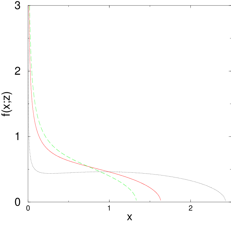
The charge density changes its shape in an interesting manner as one changes the barrier location . For the global maximum of is always at (at the barrier) where it has a integrable singularity. For , the density is non-monotonic and in addition to the square root divergence at , develops a local minimum and a local maximum respectively at . For , the density decreases monotonically with increasing . In Fig. (2) we show the behavior of for three representative values of . An interesting point about the eigenvalue distribution given Eq. (47) is that, for there is a strong accumulation of eigenvalues at the barrier location or equivalently at . In the case if one thinks of the eigenvalues as being associated about the vacuum of a (stable) field theory then there is an accumulation of modes of mass close to zero, a fact that may have consequences in the context of anthropic principal based string theory or in other physical systems where only stable configurations can be observed.
II.2 Large Deviations of the Maximum or the Minimum
Having computed the constrained charged density , we next calculate the action at the saddle point. In order to calculate from Eq. (35), we will use the explicit saddle point solution obtained in Eq. (47). In fact, one can simplify the expression of the saddle point action by using the integral equation (37) satisfied by the saddle point solution. We multiply Eq. (37) by and integrate over . Using the normalization one gets
| (52) |
where is the Lagrange multiplier to be determined. Substituting this result in Eq. (35) and the fact, we get
| (53) |
To determine the Lagrange multiplier , we put in Eq. (37). In the integral on the rhs of Eq. (37) we then make the usual shift, and use to get
| (54) |
where is explicitly given in Eq. (47) and in Eq. (48). Substituting the expression of in Eq. (53) and we finally get
| (55) |
with given explicitly in Eq. (47). The integrals can again be performed explicitly using Mathematica and using Eq. (40) we get the following expression for the saddle point action
| (56) |
The partition function is then given by Eq. (39). Note also, using Eq. (51), we have
| (57) |
where from Eq. (56). Taking the ratio in Eq. (18) gives us , the probability that all eigenvalues are to the right of
| (58) |
where is given by
| (59) |
The probability that all eigenvalues are positive (or negative) is simply
| (60) |
where
| (61) |
Finally let us turn to the large deviation function associated with large negative fluctuations of of to the left of its mean value . Substituting the expression for from Eq. (58) in Eq. (15) we get
| (62) |
Noting that , it is useful to center the distribution around the mean and rewrite Eq. (62) as
| (63) |
where the large deviation function with given explicitly in Eq. (59).
One can easily work out the asymptotic behavior of for small and large . For example, it is easy to see that
| (64) | |||||
In particular, when , i.e, we are rather close to the right edge of the Wigner sea (see Fig. 1), it follows that the scaling variable . Hence substituting the small behavior of from Eq. (64) in Eq. (63), it follows that in this regime
| (65) |
Note that this matches exactly with the left tail behavior of the Tracy-Widom limiting distribution for all the three cases , and [24]. For example, for , one can easily verify by comparing Eqs. (65) and (9). This is to be expected because the Tracy-Widom distribution describes the distribution of around its mean over a scale . If we want to investigate the probability of negative fluctuations of order , we need to look at the left tail of the Tracy-Widom distribution. On the other hand, those negative fluctuations of order are described by the small argument behavior of the large deviation function. These two behaviors thus should smoothly match. As we verified above, they do indeed match smoothly, thus providing another confirmation of our exact result. Moreover, our large deviation function provides an alternative way to compute the left tail of the Tracy-Widom distribution for all .
III Coulomb Gas Bounded by two walls: the joint probability distribution of and
In this section we compute, by the Coulomb gas method, the probability that all eigenvalues are in the interval where . Evidently, in the limit , which was computed in the previous section. Clearly, is also the cumulative probability that and , i.e.,
| (66) |
In other words, provides the joint probability distribution of the minimum and the maximum eigenvalue. By definition,
| (67) |
where is the joint pdf in Eq. (12). As in the previous section, this multiple integral can be written as a ratio of two partition functions
| (68) |
where
| (69) |
and is the same normalization constant as in Eq. (18). Thus, represents the partition function of the Coulomb gas that is sandwiched in the region bounded by the two hard walls at its boundaries.
We then evaluate this partition function in the large limit using the saddle point method. The formalism is exactly same as in the previous section. We first define a counting function that is nonzero only in the region and is zero outside. The rest of the calculation is similar as in the previous section, except that all the integrals run over the region where and . The action is exactly as in Eq. (35). Thus the partition function, in the large limit, behaves as
| (70) |
where the saddle point density , in terms of scaled variables and , satisfies the integral equation
| (71) |
where indicates the Cauchy principle part. Next we introduce the shift
| (72) |
and define . Since , it follows that . Thus denotes the location of the left barrier and denotes the location of the right barrier. In terms of the shifted variable, we rewrite the density field as
| (73) |
Eq. (71) then reduces to the integral equation
| (74) |
The integral equation (74) can again be solved using Tricomi’s theorem. Note that this equation has almost similar form as Eq. (44) except that the integral on the rhs of Eq. (74) runs up to . From the solution of Eq. (44) presented in Eq. (47) we learned that the density is nonzero only for and is zero for where . So, comparing to Eq. (74) we see that there are two possibilities:
(i) If , the solution will be exactly the same as presented in Eq. (47). In this case, the Coulomb gas does not feel the presence of the right barrier at . In other words, the solution is completely independent of and one can effectively put , i.e., put the right barrier at infinity. Thus in the case, the charge density diverges as at the left barrier and vanishes at .
(ii) If , then the solution will be given by Eq. (46) with replaced by . Using in Eq. (46) and performing the integral on the rhs we get
| (75) |
where is an arbitrary constant. The normalization condition, , fixes the constant . In this case, the charge density diverges (with a square root singularity) at the locations of both the left barrier () and the right barrier ().
Thus, putting (i) and (ii) together, we find that the solution for the equilibrium charge density for the Coulomb gas sandwiched between two barriers is given by
| (76) |
where
| (77) |
Clearly, in the limit , we indeed recover the results of the previous section. Summarizing, if one fixes the left barrier at and varies the position of the right barrier (equivalently by varying the distance between the two walls), one finds that the charge density at the left barrier always diverges. On the other hand, the behavior of the density near the right barrier undergoes a sudden change as increases beyond a critical value . The density at the right wall diverges as long as , i.e., . But when or equivalently , the charge density goes to zero at the right edge of the support at .


Having determined the charge density , the saddle point action , is then determined via the following equation that is analogous to Eq. (55)
| (78) |
where and and are given respectively in Eqs. (76) and (77). Denoting the saddle point action and evaluating explicitly the integrals in Eq. (78) we get for
| (79) |
For , becomes independent of and sticks to its value . On the other hand, we know that when , must be equal to the action for a single wall as given in Eq. (56). Indeed, one can check explicitly that , thus confirming the expectation.
The partition function, in terms of the scaled variables and , then follows from Eq. (70)
| (80) |
Note that the denominator in Eq. (67) is still given by Eq. (57) where . Hence taking the ratio in Eq. (67) and using Eq. (80) we get the joint probability for large
| (81) |
where
| (82) |
with given by Eq. (79). One can check easily that when the second wall moves to infinity, i.e., , where is given in Eq. (59). Thus, Eq. (81) for the joint distribution of and is a generalization of Eq. (58) that describes only the distribution of .
IV Numerical Results
The reader will realize that the numerical confirmation of the analytical results of the previous section is a delicate and potentially computation intensive task. For simplicity we will restrict our selves to the case of the GOE but the methods used can be extended to the other ensembles. The simplest way to compute the probability that all eigenvalues are greater than some value is to numerically generate matrices from the required ensemble, diagonalize them and then count the number that satisfy the eigenvalue constraint required. However because of the order suppression of this probability found here, for large the number of matrices that one would need to generate before seeing a single matrix satisfying the constraint is huge. The estimate for the probability that all eigenvalues are positive in this method is given by
| (83) |
In [4] an approximate argument for the GOE () was made yielding and a subsequent numerical study on matrices up to with an -dependent fit yielded and [25] was found. However given that there are corrections and the size of the systems studied are so small this fit cannot be taken too seriously. In fact one can use the Coulomb gas representation of the eigenvalues of Gaussian ensembles in order to numerically compute for much larger values of . However as a test of this method for smaller values of we may adopt the direct enumeration approach of [4] but slightly improve it to gain a few extra values of .
If the all the eigenvalues of a matrix are positive then for any vector we must have that
| (84) |
In particular if we choose the vector to be one of the basis vectors then Eq. (84) implies that
| (85) |
and so if is positive (in the operator sense), all of the diagonal elements must be positive. The estimation of can thus be slightly improved by increasing the chances of seeing a positive matrix by forcing the diagonal elements to be positive. With respect the the simplest form of enumeration, the matrices generated are the same as those for the GOE but the diagonal elements are replaced with their absolute value. The probability that a given matrix has all diagonal elements positive is , thus if denotes the number of these so generated matrices (with positive diagonal elements) then the estimation of the probability that a GOE matrix is positive is given by:
| (86) |
For small this method thus appreciably increases the probability of generating positive matrices and thus enhances the accuracy of the estimate for . Even so using this method it is virtually impossible to obtain meaningful results for . The results obtained by this modified enumeration method are shown on Fig. (4) (squares).
For large it is in fact much better to evaluate directly from Eq. (18) via a Monte Carlo method. We note that we can write
| (87) |
where and the angled bracket indicates the average is over taken to be independent and Gaussian of zero mean and unit variance. The term can also be related to the expectation over which are similarly independent and Gaussian of zero mean and unit variance but conditioned to be positive, and we denote the average of with respect to these variables by . We find that
| (88) |
the left-hand side now has has the form of a conditional average, the factor of giving the correct normalization for the conditioned probability distribution. Putting all this together yields
| (89) |
The two expectation values can be computed via Monte Carlo sampling, the unconditioned one by using Gaussian random variables and the second trivially by using the absolute value of Gaussian random variables. Shown in Fig. (4) is a plot of for the GOE () ensemble measured as described above (circles), we see that the agreement for small with the results obtained by modified enumeration approach is excellent. For larger values of we have used Monte Carlo samplings and there is a significant amount of fluctuation as indicated by the error bars. The Monte Carlo results were fitted using the fit a fit , for values of between and , the fit yields , and which is in good agreement with that predicted here. However given the errors for large and the fact that there are probably corrections of , the numerical estimate for the exponent probably on has about a 10 % accuracy.
Also, by direct sampling over Gaussian matrices, one can numerically evaluate the the rescaled density for states for matrices having only positive eigenvalues. Because we use the direct sampling method we are clearly restricted to small values of , however in Fig. (5) we show the analytical large result for with that computed numerically for matrices with and for , we see that despite the small value of the agreement is already rather good, the main deviation being in the tails for large .
V Conclusions
In this paper we have shown how the Coulomb gas formulation of the distribution of eigenvalues of Gaussian random matrices can be exploited to derive exact asymptotic results concerning the extreme value statistics of their eigenvalues. Our main results are summarized as follows.
We have shown the probability that all eigenvalues are positive (or negative) (or equivalently the probability that or ) decays as for large where and is the Dyson index.
More generally, we have computed the probability that the maximal eigenvalue is located deep within the Wigner sea region, far to the left from its average value , i.e., when . This probability has the asymptotic form, for large , where the large deviation function has been computed exactly.
We have also computed the asymptotic joint probability distribution of and .
Our result in (ii), valid when (deep inside the Wigner sea) is complimentary to the Tracy-Widom [9] result that concerns the distribution of about its mean value (near the edge) over a small range of width , i.e., for . We have demonstrated explicitly how these two results match up smoothly as one approaches from deep inside the Wigner sea to its right edge.
The key step in our method for computing the distribution of (or ) in (ii) consists in using a functional integral approach to study the Coulomb gas representation of the problem and imposing a single hard wall constraint which enforces the fact that no eigenvalues can be to the left (or right) of a given point. For the computation of the joint distribution of and in (iii), we needed to confine the Coulomb gas within two hard walls. In the limit of large , the functional integrals can be evaluated by the saddle point method and the resulting integral equations for the saddle point density can be solved explicitly using Tricomi’s theorem [23].
Our method is actually rather general and has already been adapted to study the critical points of Gaussian random fields in large dimensional spaces [19, 20] and the extreme value statistics of the maximum eigenvalue of Wishart random matrices [21]. One can possibly find further applications in related statistical problems. For instance the method is probably adaptable to study the statistics of the index (the number of negative eigenvalues) [6] of random matrices and one could also study the extreme value statistics of the minimal value of the modulus of the eigenvalues by introducing the the appropriate constraint on the density of eigenvalues in the functional integral formulation of the problem.
Note that in this paper we were able to compute only the leading large behavior of the distribution of extreme eigenvalues. It would be interesting to compute the sub-leading corrections to this leading behavior. Some recent attempts have been made in this direction [26].
Acknowledgments We would like to thank V. Osipov for useful discussions and for explaining his preliminary results with E. Kanzieper.
References
- [1] E.P. Wigner, Proc. Cambridge Philos. Soc. 47, 790 (1951).
- [2] M.L. Mehta, Random Matrices, 2nd Edition, (Academic Press) (1991).
- [3] L. Susskind, arXiv:hep-th/0302219; M.R. Douglas, B. Shiffman, and S. Zelditch, Commu. Math. Phys. 252, 325 (2004).
- [4] A. Aazami and R. Easther, J. Cosmol. Astropart. Phys. JCAP03 013 (2006).
- [5] J-P. Dedieu and G. Malajovich, arXiv:math/0702360.
- [6] A. Cavagna, I. Giardina and J.P. Garrahan, Phys. Rev. B, 3960 (2000).
- [7] Y.V. Fyodorov, Phys. Rev. Lett. 92, 240601 (2004); ibid Acta Phys. Polonica B 36, 2699 (2005).
- [8] D.S. Dean and S.N. Majumdar, Phys. Rev. Lett. 97, 160201 (2006).
- [9] C.A. Tracy and H. Widom, Commun. Math. Phys. 159, 151 (1994); ibid 177, 727 (1996).
- [10] S.N. Majumdar, Les Houches lecture notes on ‘Complex Systems’, 2006 ed. by J.-P. Bouchaud, M. Mézard and J. Dalibard (also available in arXiv:cond-mat/0701193).
- [11] J. Baik, P. Deift, and K. Johansson, J. Am. Math. Soc. 12, 1119 (1999).
- [12] J. Baik and E.M. Rains, J. Stat. Phys. 100, 523 (2000); K. Johansson, Commun. Mat. Phys. 209, 437 (2000).
- [13] M. Prahofer and H. Spohn, Phys. Rev. Lett. 84, 4882 (2000); J. Gravner, C.A. Tracy, and H. Widom, J. Stat. Phys. 102, 1085 (2001); S.N. Majumdar and S. Nechaev, Phys. Rev. E 69, 011103 (2004); T. Imamura and T. Sasamoto, Nucl. Phys. B 699, 503 (2004).
- [14] S.N. Majumdar and S. Nechaev, Phys. Rev. E 72, 020901(R) (2005).
- [15] M.G. Vavilov, P.W. Brouwer, V. Ambegaokar, and C.W.J. Beenaker, Phys. Rev. Lett. 86, 874 (2001); A. Lamacraft and B.D. Simons, Phys. Rev. B 64 014514 (2001); P.M. Ostrovsky, M.A. Skvortsov, and M.V. Feigel’man, Phys. Rev. Lett. 87, 027002 (2001); J.S. Meyer, and B.D. Simons, Phys. Rev. B 64, 134516 (2001); A. Silva and L.B. Ioffe, Phys. Rev. B 71, 104502 (2005); A. Silva, Phys. Rev. B 72, 224505 (2005).
- [16] G. Biroli, J-P. Bouchaud, and M. Potters, Europhys. Lett. 78, 10001 (2007).
- [17] R.M. May, Nature, 238, 413 (1972).
- [18] E. Kussell and S. Leibler, Science 309, 2075 (2005).
- [19] A.J. Bray and D.S. Dean, Phys. Rev. Lett. 98, 15021 (2007).
- [20] Y.V. Fyodorov, H-J. Sommers, and I. Williams, JETP Lett. 85, 261 (2007). Y.V. Fyodorov and I. Williams, arXiv:cond-mat/0702601.
- [21] P. Vivo, S.N. Majumdar and O. Bohigas, J. Phys. A: Math. Theor 40, 4317 (2007).
- [22] F.J. Dyson, J. Math. Phys. 3, 140; ibid 157; ibid 166 (1962).
- [23] F.G. Tricomi, Integral Equations (Pure Appl. Math. V, Interscience, London 1957); S.L. Paveri-Fontana and P.F. Zweifel, J. Math. Phys. 35, 2648 (1994).
- [24] While in principle the contributions could have possibly modified this limiting behaviour, the agreement with the Tracy-Widom asymptotics shows that clearly this is not the case.
- [25] There is clearly a misprint in the sign of exponent of given for this fit in [4].
- [26] V.A. Osipov and E. Kanzieper, unpublished.