Analyzing the Topology Types arising in a Family of Algebraic Curves Depending On Two Parameters
Abstract
Given the implicit equation of a family of algebraic plane curves depending on the parameters , we provide an algorithm for studying the topology types arising in the family. For this purpose, the algorithm computes a finite partition of the parameter space so that the topology type of the family stays invariant over each element of the partition. The ideas contained in the paper can be seen as a generalization of the ideas in [3], where the problem is solved for families of algebraic curves depending on one parameter, to the two-parameters case.
,
1 Introduction
The computation of the topology of algebraic sets is an active research topic. In this sense, the topology of plane algebraic curves has been extensively addressed (see [6], [14], [16], [17] and many others). More recently, the computation of the topology of space algebraic curves (see [4], [11], [13], [23]) and of algebraic surfaces (see [10], [12], [15]) has also been studied; furthermore, related to the topological study of surfaces, the problem of determining the topology types arising in the family of level curves of an algebraic surface has been considered by some authors (see [3], [5], [22]) under different perspectives. Clearly, this last problem is analogous to the question of determining the topology types appearing in a family of plane algebraic curves depending on a parameter. In addition, in [19] the authors solve the problem of determining the solutions of a zero-dimensional polynomial system depending on several parameters; this problem can be interpreted as the computation of the topology types of a zero-dimensional variety, depending on several parameters.
In this paper we address the problem of studying the topology types arising in a family of plane algebraic curves depending algebraically on two parameters. From Hardt’s Semialgebraic Triviality Theorem (see Theorem 5.46 in [8]), it is known that the number of topology types arising in such a family is finite. In order to determine them, here we provide an algorithm that determines a partition of the parameter space so that the topology type of the family is constant over each element of the partition. The algorithm generalizes the ideas in [3] (where families of algebraic curves depending on one parameter are considered) to the two-parameters case.
More precisely, in [3] it is proven that, given the implicit equation of a family of algebraic curves depending on the parameter , the parameter values where the topology type of the family may change are contained in the set of real roots of a double discriminant of ; so, in between two consecutive real roots of this polynomial, the topology type of the family stays the same (see Subsection 2.1 for more details). Thus, a finite partition of the parameter space (, in this case) with the property that the topology type stays invariant over each element of the partition, is derived. When the family depends not on one, but on two parameters, the double discriminant is a polynomial in two variables (the parameters), and therefore it defines an algebraic variety over . Hence, the geometry of this variety has to be analyzed in order to compute a decomposition of the parameter space (in our case, ) with similar properties. In this sense, the main result of this work is an algorithm for computing a partition of into cells of dimensions so that the topology type of the family stays invariant along each cell. For this purpose, the tools that we use are, essentially, McCallum’s notion of delineability (see [7]), properties of resultants and its specialization, and properties of analytic functions in several variables and germs, basically taken from [1] and [18].
The structure of this paper is the following. In Section 2, we review the main ideas for the one-parameter case, we recall the notion of delineability and some related results, and we introduce some notation and hypotheses for the two-parameters case. In Section 3 we thoroughly analyze the two-parameters case and we give a full algorithm. In Section 4 we present some examples illustrating the algorithm.
2 Preliminaries
2.1 Topology of families of algebraic curves depending on a parameter
Let be a polynomial not containing any factor just depending on the variable . Thus, defines a family of plane algebraic curves depending on the parameter , i.e. for all , defines an affine plane algebraic curve . We say that two members , of the family have the same topology type, if there exists an homeomorphism of the plane into itself transforming into ; in that case, it follows that the curves defined by , have the same shape. Then, one may address the problem of determining the topology types arising in the family. In [3], an analogous problem, namely the computation of the topology types arising in the family of level curves to a given algebraic surface, is considered. So, in the sequel we will recall the main ideas in [3].
First of all, we assume that the following hypotheses on the family hold: (i) contains no factor only depending on the variable ; (ii) is square-free; (iii) the leading coefficient of w.r.t. the variable does not depend on the variable . Note that (iii) can always be achieved by applying if necessary a change of coordinates of the type , which does not change the topology of the family. Furthermore, we consider the following definition:
Definition 1
Let be a finite subset , and let where . Moreover, let , . We say that is a critical set of the family defined by , if given verifying that , the topology types of and are equal.
In other words, a critical set of a family is a finite real set containing all the parameter values where the topology type may change.
Now let us introduce the following two polynomials; here, , and denotes the square-free part of . Also, abusing of language, in the sequel we will refer to as the “discriminant” of w.r.t. the variable (notice that usually the discriminant denotes the result of dividing out the resultant by the leading coefficient). Then we define
Furthermore, when , and when . Then the following theorem holds (see [3] for a proof of this result).
Theorem 2
Let satisfy the preceding hypotheses. Then the following statements hold:
- (1)
If is not identically zero, then the set of real roots of , is a critical set of . If has no real roots, then the elements of the family show just one topology type.
- (2)
If is identically zero, then there are two possibilities:
- (i)
, in which case ; here, the set of real roots of is a critical set.
- (ii)
, but ; here, the set of real roots of is a critical set.
- (i)
The elements of a critical set induce a finite partition of the parameter space (, in this case). The elements of this partition are, on one hand, the , and on the other hand, the intervals . So, each element of the partition gives rise to one topology type. In order to describe these topology types, it suffices to consider one -value for each element of the partition; then, the topologies of the corresponding curves can be described, for instance, by using the algorithm in [16], [17].
Furthermore, if is square-free (which typically happens when is non-sparse) then is an iterated discriminant; then, results on the structure of iterated discriminants (see [9] and [20]) can be applied in order to efficiently compute the real roots of .
Moreover, by using basic properties of resultants one may easily see that the following lemma, that will be used later on the paper, holds. This result provides a geometrical interpretation of the polynomial defined above. Here, we use the following definition of regular, critical and singular point of a plane algebraic curve; namely, given a polynomial and a point verifying that , we say that it is: (i) regular, if ; (ii) critical, if ; (iii) singular, if .
Lemma 3
If is a critical point of the curve defined by , then .
Furthermore, Lemma 3 provides the following corollary. Here, we consider the algebraic surface defined by the polynomial in the Euclidean space with coordinates . This result will be useful in the next section.
Corollary 4
Assume that , and let be the curve defined by the polynomial on the -plane. Moreover, let be the set of real roots of , and let so that . Then every singular point of with projects onto the -plane as a point of .
2.2 Preliminaries on delineability
In [3], we used as a fundamental tool the notion of delineability; in this paper, we will also make use of this notion and of some related results, proven in [3], that we summarize in this subsection.
Essentially, a square-free polynomial is said to be delineable over a manifold (for example, an open subset), if the zero set of over is the disjoint union of the graphs of several analytic functions , where . A more detailed definition, taken from [7], is given now.
Definition 5
Let denote the -tuple . An -variate polynomial over the reals is said to be (analytic) delineable on a submanifold of , if it holds that:
- 1.
the portion of the real variety of that lies in the cylinder over consists of the union of the function graphs of some analytic functions from into .
- 2.
there exist positive integers such that for every , the multiplicity of the root of (considered as a polynomial in alone) is .
Furthermore, the in the condition 1 of the definition above are called real roots of over .
Moreover, in [7] a sufficient condition for a polynomial to be delineable is provided (see pp. 246 in [7]). This condition is used in [3] in order to prove the following result (see Section 4 of [3] for a proof of the statements in this lemma); here, we recall the definitions of the polynomials and stated in the preceding subsection.
Lemma 6
Assume that is not identically , and let be the real roots of . Then the following statements are true:
- (1)
The polynomial is delineable over each . The real roots of over each interval are denoted as and the graphs of the are denoted as .
- (2)
The polynomial is delineable over each . The real roots of over , are denoted as ; the graphs of the ’s are denoted as .
- (3)
The polynomial is delineable over each open region
The real roots of over these regions are denoted as ; the graphs of the ’s are denoted as .
Similar results hold when . In Figure 1, you may see the geometrical meaning of the functions in the statement of Lemma 6. In this picture it is implicitly assumed that the ’s and the ’s join properly, in the sense that the topological closure of a contains just one . This result is rigorously proven in [3] (see Lemma 11 in [3]). A straightforward consequence of this fact and of delineability properties is the following lemma, which will be important for our purposes.
Lemma 7
Assume that , and let be the real roots of . Then along each interval , the relative positions of the ’s, the ’s, and of the ’s w.r.t. the ’s, stay invariant.

A similar result holds when . Finally, we recall from [21] the following result, which will be used later (see Theorem 2.2.3 and Theorem 2.2.4 in [21] for a proof)
Lemma 8
The ’s, the ’s and the ’s are connected sets.
2.3 Hypotheses and notation.
In our paper we consider the two-parameters case (see Section 3). So, in this subsection we introduce the required hypotheses and notation for this case. Thus, in the sequel we assume to be working with a square-free polynomial , containing no factor only depending on the parameters , and where the leading coefficient of w.r.t. the variable does not depend on the variable . As in the one-parameter case, this last condition can always be achieved by applying if necessary an affine transformation involving only . Also, in the sequel we will denote the substitution , as . Analogously, and will denote the substitutions , , respectively; note that, since by assumption contains no factor only depending on , and cannot be the zero polynomial. Hence, (resp. ) defines a family of algebraic curves depending on the parameter (resp. ); therefore, according to the notation introduced in Subsection 2.1, for these families we would obtain polynomials (resp. ) so that the set of real roots of (resp. ) would be a critical set of (resp. ).
In addition, as in the one-parameter case, we define the following two polynomials:
Furthermore, when , and when . The relationship between the specialization of these polynomials in (resp. ) and the polynomials (resp. ) defined before, is analyzed in Subsection 3.1.
Also, whenever the polynomial is not identically 0, by applying if necessary a linear change of coordinates just involving one may also assume that the leading coefficient with respect to of the resultant does not depend on . This assumption will be needed in Subsection 3.3.
3 The two-parameters case
Here, we consider the problem of analyzing the topology types arising in a family of algebraic curves depending on two parameters. Thus, along this section we assume that we are working with a family defined by , where are parameters, and satisfies the hypotheses made explicit in Subsection 2.3. In order to solve our problem, first we will focus on the case when the polynomial defined in Subsection 2.3 is not identically zero; the special case when it is the zero polynomial will be treated at the end of the section. Under this assumption, the curve defined by the polynomial divides the real plane, with coordinates , into finitely many open regions, namely the connected components of (for example, in Fig. 2 the curve plotted there divides the plane into three open regions). Notice that, by computing a C.A.D. of , these regions correspond to the union of finitely many 2-dimensional cells which can be described from the C.A.D. Thus, we will prove that:
- (i)
- (ii)
The statement (i) follows from good specialization properties of and , which are analyzed in Subsection 3.1, and Theorem 2. The statement (ii) follows from considerations on delineability, and some properties of real analytic functions. Observe that from (i) and (ii), a partition of the parameter space (, in this case) such that the topology of is invariant over each element of the partition, is computed.
3.1 Good specialization properties of and
The aim of this subsection is to prove that the polynomials and specialize well out of the curve , i.e. that whenever (resp. ) is not a factor of , it holds that (resp. ); recall here the notation (resp. ) introduced at the end of Subsection 2.3. For this purpose, we begin with the following result, which can be proven by considering the Sylvester form of the resultant.
Lemma 9
Let , be the leading coefficients of and , respectively, w.r.t. the variables and , respectively (note that since by hypothesis is not identically zero, depends on , and depends on ). Then the following statements hold:
- (i)
is a factor of .
- (ii)
is a factor of ; in particular, is also a factor of .
This lemma is used for proving the following result.
Lemma 10
Let satisfy that is not a factor of , and let be the leading coefficient of w.r.t. . Then:
- (i)
; in particular, .
- (ii)
specializes well for .
- (iii)
(i.e. the specialization in ) is square-free as a polynomial in the variables .
Similarly for , where is not a factor of .
Proof. We prove the statement for ; similarly for . Now, let us see (i). For this purpose, assume by contradiction that (i) does not hold. Thus, . By the statement (ii) in Lemma 9, is a factor of ; so, implies that , and therefore divides . However, this cannot happen by hypothesis. Hence (i) follows. Now since (i) holds, we have that , and therefore the statement (ii) follows from Lemma 4.3.1, pg. 96 in [26]. Finally, since (ii) holds, in case that is not square-free we have that is identically ; so, divides and by Lemma 9 it also divides , which cannot happen by hypothesis. Therefore, (iii) holds.
From the above statement (iii), it may happen that , where is not a factor of , has a multiple factor depending only on , but it cannot have that has a multiple factor depending on . Now in order to see that whenever is not a factor of , we still need an additional property, namely that the specialization of has no multiple factor depending on . This is proven in the following lemma.
Lemma 11
Let satisfy that is not a factor of . Then it holds that:
- (i)
specializes well for .
- (ii)
is square-free as a polynomial in the variable .
Similarly for , where is not a factor of .
Proof. Let us see (i). The only case when does not specialize well for occurs when the leading coefficient of vanishes at (see Lemma 4.3.1, pg. 96 in [26]). However, by Lemma 9 in that case divides , which cannot happen by hypothesis. So, (i) holds. Now since (i) holds, if is not square-free we have that the specialization of the resultant at is identically , and therefore that ; so, divides , which cannot happen by hypothesis. Therefore, (ii) also holds. Similarly for .
Corollary 12
Let satisfy that is not a factor of . Then the following statements are true:
- (i)
- (ii)
.
Similarly for , where is not a factor of .
3.2 Behavior of the family over the connected components of
Here, we will see that the topology type of the family stays invariant along each of the connected components of . For this purpose, the following proposition is previously required.
Proposition 13
Let satisfy that is not a factor of , and let , , fulfilling that does not vanish for . Then the topology type of the family does not change for .
Proof. Since by hypothesis does not vanish for , then does not contain any factor with , i.e. does not identically vanish for . Now let be the content of with respect to , and let be the primitive part of w.r.t. to . Observe that since by hypothesis does not vanish for , then for both and define the same family. From the results in Subsection 3.1 it follows that fulfills the hypotheses of Theorem 2, and that the set of real roots of is a critical set of the family . Since does not vanish for , the result follows from Theorem 2.
The result in the following proposition is proven in an analogous way.
Proposition 14
Let satisfy that is not a factor of , and let , , fulfilling that does not vanish for . Then the topology type of the family does not change for .
Finally, the following theorem can be proven. Here, the connected components of are denoted as .
Theorem 15
The topology type of the family stays invariant along each , with .
Proof. Since is open and connected, one may always find finitely many segments , all of them lying in , verifying that: (i) each is either horizontal (in which case is constant over ) or vertical (in which case is constant over ); (ii) the end-point of is the starting-point of ; (iii) is a path lying in , and connecting the points and . Now by Proposition 13 and Proposition 14, we have that the topology type stays invariant along each . Hence, the result follows.
3.3 Topology types arising over
If is not square-free one can always get rid of multiple factors and keep its square-free part. Thus, in the sequel we assume that is square-free. Moreover, we also assume that is not a univariate polynomial. Observe that if (similarly if ), then we just have to study the uniparametric families where the ’s are the real zeroes of ; this can be done by applying the results in Subsection 2.1. Now let be the real zeroes of the discriminant of w.r.t. to the variable , where , and let . Then, from [7] (see pp. 246 in [7]) one may see that is delineable over each interval , i.e. that over there exist real analytic functions (namely, the real roots of over ) verifying that the graph of over is the union of the non-intersecting graphs of the (see Subsection 2.1 for more information on delineability). In other words, each corresponds to a different analytic branch of over .
Moreover, let
One may see that since by hypothesis has no factor only depending on , this polynomial is not identically . Nevertheless, may contain univariate factors depending on , that correspond to univariate factors of . These factors give rise to uniparametric families that can be analyzed separately by applying the results in Subsection 2.1; also, notice that the ’s are also real roots of . We denote by the polynomial obtained by removing the factors from . Since, from Subsection 2.3, one may assume that the leading coefficient of with respect to does not depend on , we have that the polynomial verifies the hypotheses of Theorem 2. So, let be a critical set of the uniparametric family of parameter defined by , and let ; we assume that the elements in are increasingly ordered. Moreover, in the sequel we consider an interval verifying that ; so, in particular is delineable over and therefore over the graph of is the union of several analytic branches . In this situation, the main result of this subsection is the following.
Theorem 16
Assume that is delineable over an interval , and let be the real roots of over . Then along each , with , the topology type of the curves defined by , with , stays invariant.
In other words, the theorem states that, whenever one moves along an analytic branch of in between two consecutive elements of , the topology type of the family is preserved. Thus, a finite partition of into 1-dimensional and 0-dimensional cells can be computed so that the topology type of the family remains invariant along each element of the partition. The result is illustrated in Figure 2; in this picture, . The rest of the subsection is devoted to proving this result.

In order to prove the theorem, some previous results are needed. The first result states that the zero-set of over can be expressed as the union of certain analytic functions.
Lemma 17
Let . Then, there exist different analytic functions so that the zero set of over is the union of the zero-sets of the functions , .
Proof. of these functions are the real roots of over . The existence of the remaining (complex) functions follows, for instance, from the complex version of the Implicit Function Theorem (see p. 84 in [1]) and analytic continuation.
In fact, from the complex version of the Implicit Function Theorem it follows that the ’s are defined over open complex subsets (containing ); so, is defined over an open complex subset whose -projection contains . Now Lemma 17 is required for proving the following result.
Lemma 18
The zero set of over (i.e. the zero set of whose -projection is ) is the union of the zero-sets over of the functions (in the sequel, ), .
Proof. By definition the zero set of over is the zero set over of , where is the result of removing from the univariate factors depending on . From Lemma 17 and properties of the resultant (see property 3, page 255 in [25]) we have that . Then removing the univariate factors corresponding to we get that zero set of coincides with that of .
Let be the projection onto of the open subset . Then, one may see that for , is analytic over (because it is the composition of two analytic functions, namely and ), and writing , so is ; notice that contains . Hence, for each point there exists an open (complex) subset so that has can be expanded as a power series convergent in ; in this situation, we say that defines a germ over (i.e. the zero set of over , see [18] or [1] for further information on germs). Moreover, because of Lemma 18, defines the same germ. Now the following lemma is the key for proving Theorem 16. Here we will use some ideas and results from Analytic Geometry related to germs. Namely, we will use the notion of irreducible germ, and the fact that every germ can be uniquely written as an “irredundant” union of irreducible germs (i.e. as a finite union of all-distinct, irreducible germs). We refer to Chapter V of [1] and Chapters 3, 4 of [18] for further reading on these questions. Also, we will use the following notation, analogous to the notation in Lemma 6 (see Subsection 2.2). Here we have tried to simplify the description in order to avoid a cumbersome notation.
- •
The real roots of the square-free part of the discriminant over are denoted as ’s (observe that since contains no point of the critical set of , from Lemma 6 the square-free part of is delineable over ); the graph of is denoted as .
- •
From Lemma 6, is delineable over each . The real roots of over are denoted as ’s; the graph of is denoted as .
- •
We denote by the region of the -plane lying in between two consecutive ’s, with . Also from Lemma 6, we have that is delineable over . The real roots of over are denoted as ’s; the graph of is denoted as .
Hence, the following lemma holds. Essentially, this result ensures that each is associated with some ’s, and conversely. The first statement of this lemma is illustrated in Figure 3.
Lemma 19
The following statements hold:
- (a)
Let be a real root of over a region . Then there exists , satisfying that .
- (b)
Let , and let . If vanishes at , then .
Proof. Let us see first the statement (a). From Lemma 18, it follows that is included in the zero-set of . Moreover, each is analytic over , and . So, for each point there exists an open complex subset containing so that each , and therefore also , defines a germ over ; in the rest of the proof we will refer to these germs as the “zero sets” of , over , respectively. Furthermore, since by Lemma 8 is connected, we can always take sufficiently small so that is also connected. Now, the zero-set of each over can be written as a finite union of irreducible germs (see p. 237 of [1]) . Moreover, the zero-set of over can also be written as an “irredundant” union of irreducible germs , and each is included in some , where and (see p. 240 of [1]). Let us see that there exists just one verifying that . Indeed, clearly . Now if the statement does not hold then either is not connected, which cannot happen, or there exist two different ’s, say , and a point , so that . However, since are different germs in this last case would be a self-intersection of the surface defined by , and therefore a singular point of ; but this cannot happen, either, because from Corollary 4 every singular point of with projects onto some . So, there exists so that . Then, let satisfy that , where . Hence, . Finally, since is analytic, is defined over the whole , and vanishes over , then it vanishes over the whole (see p. 81 in [18]).
In order to prove part (b), by contradiction one assumes that the statement is not true, and, reasoning as in part (a), one shows that the surface has a self-intersection not projecting onto any , which violates Corollary 4.
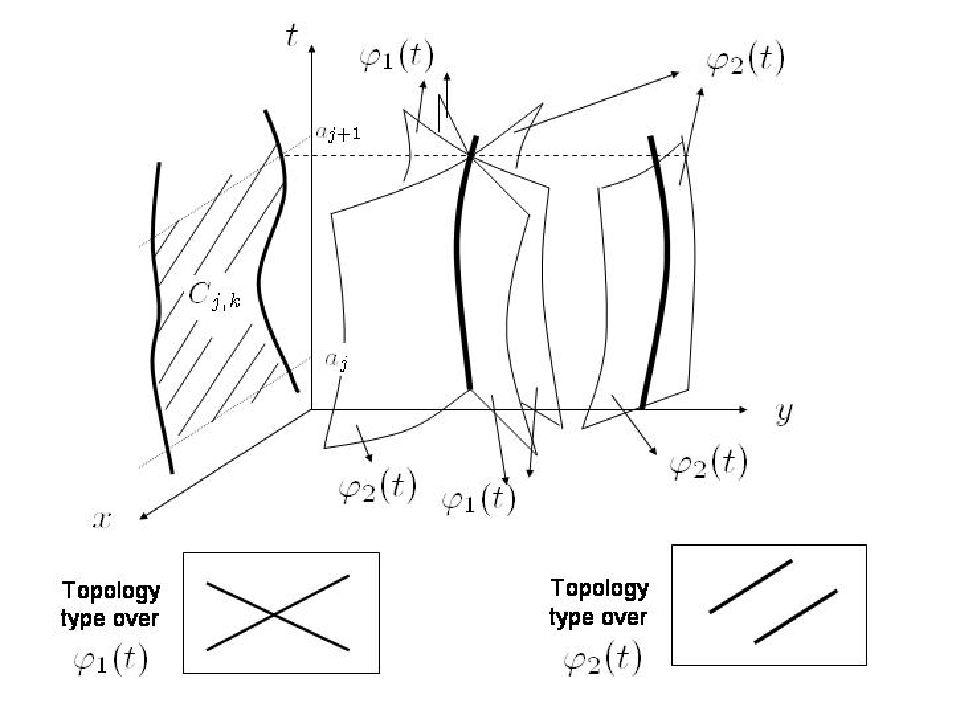
Remark 1
Notice that the appearing in the statement (a) of Lemma 19 is not necessarily unique, i.e. it may happen that given there exist so that . Moreover, part (b) of Lemma 19 essentially says that over a , two different ’s are either disjunct or fully coincident; therefore, a (i.e. its zero-set) cannot contain a part of a , but a whole .
Finally, Theorem 16 can be proven.
Proof of Theorem 16. Let , with , be a real root of over . Now from Lemma 18, the zero-set of with is included in the zero-set of . Moreover, for each region the zero-set of over is equal to the union of the ’s; then, from Lemma 19, for each region there exists a subset so that the real part of the zero-set of with and is equal to the union of the ’s with ( is empty iff has no real zero with and ). Furthermore, if and is in the closure of , then because is continuous. Finally, since by Lemma 7 the relative positions of the ’s, the ’s, and of the ’s w.r.t. the ’s stay invariant when , we have that the topology type of the level curves of with stays invariant. Hence, Theorem 16 follows.
3.4 The Algorithm
From the ideas in the preceding subsections, we can derive the following algorithm for computing a finite partition of into 0-dimensional, 1-dimensional and 2-dimensional cells so that the topology type of the family defined by stays invariant along each cell; we denote by the sets consisting of all the 0-dimensional cells, the 1-dimensional cells, and the 2-dimensional cells, respectively. Here, we assume that fulfills the hypotheses made explicit at the beginning of the section, and that . Observe that once the partition has been computed, the topology types in the family might be determined by first choosing a point in each partition element, and then applying the method in [16], [17] for describing the topology of the resulting curve. However, in some cases it can be difficult or even impossible to choose both being rational; so, in some situations we might not obtain all the topology types in the family. Still, however, we get the parameter values corresponding to each type.
Algorithm: (two-parameters case)
- 1.
[Polynomials ] Compute the polynomials .
- 2.
[Set ] Compute the real roots of , , and let be the set consisting of these values. Let be the real intervals verifying that .
- 3.
[0-dimensional cells] For all , where does not divide , compute the points verifying that . Then
Some other points may be added in Step 4.1.
- 4.
[1-dimensional cells]
- 4.1
[Univariate factors] For each where divides , compute a critical set of the family defined by . Let be the real intervals verifying that , and let . Moreover, add the points , where , to the list of 0-dimensional cells computed in Step 3.
- 4.2
[Analytic branches of ] Let be the real roots of over each , and let .
- 4.3
[List of Cells]
- 4.1
- 5.
[2-dimensional cells] Let , where denote consecutive real roots of over . Then
Observe that, from Theorem 15, if two adjacent 2-dimensional cells computed in the step (5) of the above algorithm are not separated by any 1-dimensional cell computed in the step (4), then the topology type of the family is the same over both cells; in fact, in that case both cells would correspond to the same connected component of . Notice also that two adjacent cells might give rise to the same topology type; so, the decomposition computed by the above algorithm is not necessarily minimal. Finally, observe also that, as in the one-parameter case, whenever is square-free the ideas of [9] and [20] might be used in order to more efficiently compute .
3.5 The special case
If , from the definition of it holds that either , in which case , or , in which case . In both situations the reasonings are completely analogous to the case ; so, here we state the main results for this special case and we leave the proofs to the reader.
If , we denote , which defines a curve . We denote the connected components of as . Moreover, we also denote . Hence, defines a uniparametric family, and therefore one may compute a critical set of the family. Then, the following result holds. Here, denotes the union of the real roots of and the elements of .
Theorem 20
The topology type of the family stays the same over each , and also along each real root of over each interval of lying in between two consecutive elements of .
For the case , defines a curve ; we represent the connected components of as . Moreover, we write , and we denote by a critical set of the uniparametric family defined by . Also, denotes the union of the real roots of , and the elements of . Then we have the following theorem.
Theorem 21
The topology type of the family stays the same over each , and also along each real root of over each interval of lying in between two consecutive elements of .
4 Examples.
In this section we provide three examples in order to illustrate the ideas of Section 3. The two first ones correspond to the case , while the third one corresponds to . Moreover, in the second example the topology types arising in the offset family to the parabola are computed. Offset curves (see for example [24] for more information on this subject), widely used in the CAGD context, can be intuitively described as “parallel” curves to a given curve at a certain distance. If the offsetting distance is not particularized, then the offset family to a given algebraic curve is certainly a family of algebraic curves depending on the parameter , and the topology types in the family can be computed by using the results in Subsection 2.1 (see [3] for further details); this may be useful in order to identify the distances where the topology of the offset coincides with that of the original curve, which is the desired situation in most applications. Now if the original curve depends on one parameter, as it happens in the case of , then the offset is a family of algebraic curves depending on two parameters, and therefore the results in our paper are applicable. The computation of the topology types in the offset family to was solved by Prof. W. Lü (1992) by using “ad-hoc” methods. However, here we compute them as a direct application of the general algorithm provided in Section 3.
Example 1
Consider the family of algebraic curves defined by
The curves of this family are usually known as the Cassini’s ovals. Let us see how the algorithm works in this case:
- 1.
[] The polynomial (after removing multiple factors) is
Moreover, we also get
One may see that has just one univariate factor, namely , depending on the variable . Then is immediately obtained.
- 2.
[] , have just one real root, namely ; so, .
- 3.
[0-dimensional cells] We have just one 0-dimensional cell, namely .
- 4.
[1-dimensional cells]
- 4.1
[Univariate factors] Over , the family reduces to . A critical set of this new family is . So, no new 0-dimensional cells are found, and we get two 1-dimensional cells, namely and .
- 4.2
[Analytic branches of ] When , has 5 real roots, corresponding to the cases , , , , , respectively (see Figure 4); each one gives rise to a different 1-dimensional cell. The same happens when .
- 4.1
- 5.
[2-dimensional cells] They are the two-dimensional regions lying in between consecutive real roots of over and , respectively (see also Figure 4). One may see in Figure 4 that there are 12 of these cells, named as ; also, the border between, say, and corresponds to the 1-dimensional cell defined by and , etc.
One may find the topology types corresponding to each cell also in Figure 4.

Example 2
Consider the family of parabolas defined by . One may check that the equation of the corresponding offset family is
Moreover, the computation of the double discriminant yields (after removing multiple factors):
Without loss of generality we can assume that (otherwise a degenerated situation is reached) and (the offsetting distance is never ); moreover, also w.l.o.g. we can assume that , . One can check that in this case a critical set of the polynomial reduces to ; so, we have the following cases: (1) ; (2) ; (3) ; (4) ; (5) . Furthermore, one may also check that the topology type coincides in (3), (4) and (5); so, finally we get three topology types corresponding to the cases , , , respectively, which are shown in Figure 5.
Example 3
We consider the linear system of curves defined by
Here, we get that . Thus, . Then we consider the uniparametric family defined by . Since does not depend on , from Theorem 2 we have that the set of real roots of , i.e. , is a critical set of the family. Hence, these values induce a partition of the line into four pieces, corresponding to the cases , , and , respectively. More precisely, we have the following partition of the parameter space:
- •
[0-dimensional cells]: ; here, the topology type of is that of two parallel lines (in the three cases).
- •
[1-dimensional cells]: ; ; ; ; here, the topology type is that of three parallel lines (in all the cases).
- •
[2-dimensional cells]: ; ; here, the topology type is that of a line (in both cases).
References
- [1] Abhyankar S. (1964), Local Analytic Geometry, World Scientific Co., Singapore 2001.
- [2] Alcazar J.G. (2007), Effective Algorithms for the Computation of the Topology of Algebraic Varieties, and Applications, PhD Thesis, Universidad de Alcala de Henares (Spain). Available at www2.uah.esjuange alcazar.
- [3] Alcazar J.G., Schicho J., Sendra R. (2007) A Delineability-based Method for Computing Critical Sets of Algebraic Surfaces, Journal of Symbolic Computation vol. 42, pp. 678-691
- [4] Alcazar J.G., Sendra R. (2005) Computation of the Topology of Real Algebraic Space Curves, Journal of Symbolic Computation 39, pp. 719-744.
- [5] Alcazar J.G., Schicho J., Sendra R. (2006) Shape of Level Curves of Algebraic Surfaces: Determination and Some Applications, Proceedings EACA 06
- [6] Arnon D., McCallum S. (1988). A polynomial time algorithm for the topology type of a real algebraic curve, Journal of Symbolic Computation, vol. 5 pp. 213-236.
- [7] McCallum S. (1998). An Improved Projection Operation for Cylindrical Algebraic Decomposition. In Quantifier Elimination and Cylindrical Algebraic Decomposition (Eds. B.F. Caviness, J.R. Johnson), Springer Verlag, pp.242–268.
- [8] Basu S., Pollack R., Roy M.F. (2003) Algorithms in Real Algebraic Geometry , Springer Verlag.
- [9] Buse L., Mourrain B. (2008) Explicit factors of some iterated resultants and discriminants, AMS Journal Mathematics of Computation (to appear).
- [10] Cheng J.S., Gao X.S., Li M. (2005). Determine the Topology of Real Algebraic Surfaces, Proceedings of Mathematics of Surfaces XI, 121-146, LNCS3604, Springer.
- [11] El Kahoui, Mhammed (2008), Topology of real algebraic space curves, Journal of Symbolic Computation 43, pp. 235-258.
- [12] Fortuna R., Gianni P., Luminati D. (2004). Algorithmical Determination of the Topology of a Real Algebraic Surface. Journal of Symbolic Computation 38, pp. 1551–1567.
- [13] Gatellier G., Labrouzy A., Mourrain B., Tecourt J.P. (2004) Computing the topology of three-dimensional algebraic curves. Computational Methods for Algebraic Spline Surfaces, pages 27-44. Springer-Verlag.
- [14] Gianni P., Traverso C. (1983). Shape determination of real curves and surfaces, Annali dell’ Universita di Ferrara. Sezione VII. Scienze Matematische XXIX, pp. 87-109.
- [15] Gianni P., Fortuna E., Parenti P., Traverso C. (2002). Computing the topology of real algebraic surfaces Proc. ISSAC 2002 pp. 92-100, ACM Press.
- [16] Gonzalez-Vega L., Necula I. (2002). Efficient topology determination of implicitly defined algebraic plane curves, Computer Aided Geometric Design, vol. 19 pp. 719-743.
- [17] Hong H. (1996). An effective method for analyzing the topology of plane real algebraic curves, Math. Comput. Simulation 42 pp. 571-582
- [18] Jong T., Pfister G. (2000), Local Analytic Geometry, Vieweg, Advanced Lectures on Mathematics.
- [19] Lazard D., Rouillier F. (2007), Solving parametric polynomial systems, Journal of Symbolic Computation 42, pp. 636-667.
- [20] Lazard D., McCallum S. (2007), Iterated Discriminants, Proceedings MEGA ’07.
- [21] McCallum S. (1984), An improved projection operation for cylindrical algebraic decomposition, Ph.D. Thesis, University of Wisconsin-Madison.
- [22] Mourrain B., Tecourt J. (2005). Isotopic Meshing of a Real Algebraic Surface, Rapport de recherche num. 5508, Unite de Recherche INRIA Sophia Antipolis.
- [23] Niang D., Mourrain B., Ruatta O. (2008). On the Computation of the Topology of a Non-Reduced Implicit Space Curve, Proceedings ISAAC 08.
- [24] Sendra J., Sendra J.R. (2000). Algebraic Analysis of Offsets to Hypersurfaces. Mathematische Zeitschrift vol. 234, pp. 697–719.
- [25] Sendra J.R., Winkler F., Perez-Diaz S. (2007). Rational Algebraic Curves, Springer.
- [26] Winkler F. (1996), Polynomial Algorithms in Computer Algebra. Springer Verlag, ACM Press.