Particle-hole symmetry and the dirty boson problem
Abstract
We study the role of particle-hole symmetry on the universality class of various quantum phase transitions corresponding to the onset of superfluidity at zero temperature of bosons in a quenched random medium. To obtain a model with an exact particle-hole symmetry it is necessary to use the Josephson junction array, or quantum rotor, Hamiltonian, which may include disorder in both the site energies and the Josephson couplings between wavefunction phase operators at different sites. The functional integral formulation of this problem in spatial dimensions yields a -dimensional classical -model with extended disorder, constant along the extra imaginary time dimension—the so-called random rod problem. Particle-hole symmetry may then be broken by adding nonzero site energies, which may be uniform or site-dependent. We may distinguish three cases: (i) exact particle-hole symmetry, in which the site energies all vanish, (ii) statistical particle-hole symmetry in which the site energy distribution is symmetric about zero, vanishing on average, and (iii) complete absence of particle-hole symmetry in which the distribution is generic. We explore in each case the nature of the excitations in the non-superfluid Mott insulating and Bose glass phases. We show, in particular, that, since the boundary of the Mott phase can be derived exactly in terms of that for the pure, non-disordered system, that there can be no direct Mott-superfluid transition. Recent Monte Carlo data to the contrary can be explained in terms of rare region effects that are inaccessible to finite systems. We find also that the Bose glass compressibility, which has the interpretation of a temporal spin stiffness or superfluid density, is positive in cases (ii) and (iii), but that it vanishes with an essential singularity as full particle-hole symmetry is restored. We then focus on the critical point and discuss the relevance of type (ii) particle-hole symmetry breaking perturbations to the random rod critical behavior, identifying a nontrivial crossover exponent. This exponent cannot be calculated exactly but is argued to be positive and the perturbation therefore relevant. We argue next that a perturbation of type (iii) is irrelevant to the resulting type (ii) critical behavior: the statistical symmetry is restored on large scales close to the critical point, and case (ii) therefore describes the dirty boson fixed point. Using various duality transformations we verify all of these ideas in one dimension. To study higher dimensions we attempt, with partial success, to generalize the Dorogovtsev-Cardy-Boyanovsky double epsilon expansion technique to this problem. We find that when the dimension of time is sufficiently small a type (ii) symmetry breaking perturbation is irrelevant, but that for sufficiently large particle-hole asymmetry is a relevant perturbation and a new stable fixed point appears. Furthermore, for , this fixed point is stable also to perturbations of type (iii): at the generic type (iii) fixed point merges with the new fixed point. We speculate, therefore, that this new fixed point becomes the dirty boson fixed point when . We point out, however, that may be quite special. Thus, although the qualitative renormalization group flow picture the double epsilon expansion technique provides is quite compelling, one should remain wary of applying it quantitatively to the dirty boson problem.
pacs
64.60.Fr, 67.40.-w, 72.15.Rn, 74.78.-w,I Introduction
Quantum phase transitions at zero temperature are driven entirely by quantum fluctuations in the ground state wavefunction. In many cases a crucial requirement is the presence of quenched disorder. Examples include random magnets with various kinds of site, bond,[1] or field[2] disorder; the transitions between plateaux in the two-dimensional quantized Hall effects;[3] metal-insulator,[4] metal-superconductor, and superconductor-insulator[5] transitions in disordered electronic systems; and the onset of superfluidity of 4He in porous media.[6]
In this article, we will study the quantum transitions between the superfluid (SF), the localized Bose glass (BG), and Mott insulating (MI) phases, motivated mainly by the problem of superfluidity of 4He in porous media. However, as is often the case in the study of critical phenomena, the universality class of this transition, or a straightforward generalization of it, also includes other physical phenomena, such as many aspects of quantum magnetism and superconductivity.
There have been a number of approaches to studying the SF–BG transition: mean field theories,[7] strong coupling,[8] large ,[9] real space methods,[10] quantum Monte Carlo calculations,[11, 12, 13, 14] double dimensionality epsilon-expansions,[15, 16, 17], real space renormalization group in the limit of strong disorder in one dimension,[18] renormalization group in fixed dimension,[19] and in dimensions.[20] However, none of the above methods provide a controlled analytical approach to the critical point for .
A satisfactory dimensionality expansion about the upper critical dimension for the superfluid to Bose glass transition (analogous to the epsilon expansion about for classical spin problems) does not appear to exist. In particular, we previously found[17] that the approach based on a simultaneous expansion in both the dimension, , of imaginary time (physically equal to unity), and the deviation, , of the total space-time dimensionality, , from four[15] does not yield a perturbatively accessible renormalization group fixed point, and therefore does not produce a systematic expansion for the dirty boson problem. Nevertheless it does give one a fairly detailed picture of the renormalization group fixed point and the flow structures, and produce an uncontrolled expansion for the dirty boson problem, though further work needs to be done in order to understand the analytic structure of the theory as a function of . Therefore, in spite of its poor convergence, the double dimensionality expansion still appears to provide the most flexible analytic approach to the study of the SF–BG transition, including insight into the symmetries of the fixed point. As detailed below, attention to the role of particle-hole symmetry, especially, is essential to generating correct RG flow structures. In three (and higher) dimensions, the double dimensionality expansion is the only method that has been able, with partial success, to access the critical fixed point and obtain critical exponents.[17]
I.1 Particle-hole symmetry
As stated, it will transpire that an essential ingredient that is necessary in order to correctly understand the physics of the SF–BG transition is an extra “hidden” symmetry, which we call particle-hole symmetry, that is present at the critical point, but not necessarily away from it. To make this notion precise, we compare the following two lattice models of superfluidity: the first is the usual lattice boson Hamiltonian,
| (1) | |||||
where is the hopping matrix element between sites and , which we will allow to have a random component; is the chemical potential whose zero we fix by choosing the diagonal components, , of in such a way that for each ; is a random site energy with mean zero; is the pair interaction potential, assumed for simplicity to be nonrandom and translation invariant; the only nonzero commutation relations are , and is the number operator at site .
The second model is the Josephson junction array Hamiltonian,
| (2) | |||||
with analogous parameters, but now the commutation relations . These two Hamiltonians are, in fact, very closely related. It is easy to check that if is any positive integer then
| (3) |
satisfy the correct Bose commutation relations, and we identify . Note, however, that the commutation relations between and permit to have any integer eigenvalue, positive or negative, whereas the eigenvalues of must be non-negative. Therefore it is only when is large, and the fluctuations in are small compared to , that and may be compared quantitatively: inside the hopping term we may approximate , and make the identifications
| (4) |
where and , and there exists an overall additive constant term , where is the number of lattice sites.
Despite this asymptotic equivalence at large , the Josephson Hamiltonian (2) has an exact discrete symmetry which the boson Hamiltonian lacks. Thus the constant shift, , where is any integer, has no effect on the commutation relations or the eigenvalue spectrum of the . The Hamiltonian correspondingly transforms as
| (5) |
where , and . The free energy density, , where , transforms as
| (6) |
independent of the and . This implies that the only effect of a shift in the chemical potential is a trivial additive term in the free energy which is linear in . This term serves only to increase the overall density, , by but otherwise has no effect whatsoever on the phase diagram, which therefore will be precisely periodic in , with period .
Consider next the transformation , . The Hamiltonian transforms as
| (7) |
so that
| (8) |
Combining the two symmetries (6) and (8) we see that if all , then for , where is any integer, the Hamiltonian possesses a special particle-hole symmetry, namely invariance under the transformation , . At the density is precisely per site, and the thermodynamics is symmetric under addition and removal of particles (the removal of particles being synonymous with the addition of holes). If the are nonzero, but have a symmetric probability distribution, , then the exact particle-hole symmetry is lost, but there still exists a statistical particle-hole symmetry at the same special values of : self averaging will ensure that . The lattice boson Hamiltonian (1) clearly can never possess either form of particle-hole symmetry since the hopping term mixes the number and phase in an inextricable fashion.


I.2 Phase diagrams
In Fig. 1 we sketch zero temperature phase diagrams, with and without various types of disorder, in the - plane, where is a measure of the overall strength of the hopping matrix (e.g., ), in the simplest case of onsite repulsion only:[21] . This phase diagram has been discussed in detail previously[6, 11] for the lattice boson Hamiltonian, . Here we emphasize the features unique to , namely the periodicity in , and the special points corresponding to local extrema in the phase boundaries.
I.2.1 Phase diagram for the pure system
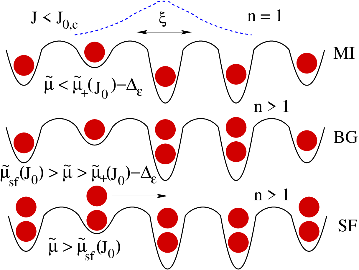
In Fig. 1(a) we show the phase diagram in the absence of all disorder. For the site occupancies are good quantum numbers and each site has precisely particles for . The points for integer are fold degenerate with either or particles placed independently on each site. For communication between sites occurs and the effective wavefunction for each particle spreads to neighboring sites (see Fig. 2). We denote by (to be defined carefully later) the range of this spread. One can show within perturbation theory,[6] however, that for sufficiently small, short ranged , there is a finite energy gap for addition of particles, and the overall density remains fixed at for a finite range of .

Consider first . Then only at a critical value of does the system favor adding extra particles (or holes). Equivalently, for a given there is an interval of fixed density . These extra particles may be thought of as a dilute Bose fluid moving atop the essentially inert background density, (see Fig. 2). The physics is identical to that of a dilute Bose gas in the continuum, and is well described by the Bogoliubov model.[22] From this one concludes that the system immediately becomes superfluid (recall that we assume ) with a superfluid density , and an order parameter . The characteristic length in this phase is and represents the distance between “uncondensed” particles: . This zero-temperature superfluid onset transition is therefore trivial, in the sense that all exponents are mean-field-like. In fact, historically this onset was never really viewed as an example of a phase transition.
Furthermore, although all quantities vary continuously as decreases toward , the actual onset point is entirely noncritical. Thus, for a given value of within a Mott lobe, the interval represents a single unique (incompressible) thermodynamic state. Incompressibility implies that for the given (integer) density, the value of the chemical potential is ambiguous. One might just as well set , its value at the center of the lobe. The correlation length, , is independent of , and remains perfectly finite in the Mott phase at . In this sense the transition has some elements of a first order phase transition.
The more important transition is the one occurring at fixed density, , at through the tip of the Mott lobe at . At this transition diverges continuously with a characteristic exponent, . One may show (see Ref. 6 and below) that the transition is precisely in the universality class of the classical -dimensional -model. What distinguishes this transition from the previous ones is precisely particle-hole symmetry: superfluidity is achieved not by adding a small density of particles or holes atop the inert background, but by the buildup of superfluid fluctuations within the background, to the point where particles and holes simultaneously overcome the potential barrier and hop coherently without resistance. The exponent exhibits itself in the phase diagram as well: a scaling argument shows that the shape of the Mott lobe is singular near its tip,[6] . In , , while in , . This will be discussed in a more general scaling context in Sec. IV.2.
We have already observed that the lattice boson Hamiltonian (1) never has an exact particle-hole symmetry. Nevertheless, one still has Mott lobes (now asymmetric and decreasing in size with increasing ) for each integer density, and a unique extremal point, , at which one exits the Mott lobe at fixed density . One may show[6] that the transition through these extremal points is still in the -dimensional universality class, and that particle-hole symmetry must therefore be asymptotically restored at the critical point. The difference now is that there is a nontrivial balance between the densities of particle and hole excitations, and the interactions between them. The position of the critical point is no longer fixed by an explicit symmetry, but must be located by carefully tuning both the hopping parameter and the chemical potential.
This phenomenon of “asymptotic symmetry restoration” at a critical point is actually fairly common (and we shall encounter it again below). For example, though the usual Ising model of magnetism has an up-down spin symmetry, the usual liquid–vapor or binary liquid critical points do not. However the Ising model correctly describes the universality class of the transition, and one concludes that the up-down symmetry must be restored near the critical point. Similarly, the -state clock model with Hamiltonian
| (9) |
which may be thought of as a kind of discrete -model, has for sufficiently large (specifically, in ; clearly corresponds to the Ising model and to the three-state Potts model) a transition precisely in the -model universality class. Note, however, that in the ordered phase, corresponding to the zero temperature fixed point, the order parameter will (for ) spontaneously align along one of the equivalent directions, , breaking the -symmetry and generating a mass for the spin-wave spectrum (more interestingly, in a power-law ordered Kosterlitz-Thouless phase exists for a finite temperature interval below the transition, with a second transition to a long-range ordered phase taking place only at a lower temperature [23]). This latter property is not relevant in the present case since breaking particle-hole symmetry does not break the symmetry of the order parameter: the nature of the superfluid phase is unaffected.
I.2.2 Phase diagrams with disorder
We will consider two types of disorder: (i) onsite disorder in the , and (ii) disorder in the hopping parameters, . If for any , that is if particle-hole symmetry is broken, we expect the two types of disorder to yield the same type of phase transition. In renormalization group language, each in isolation will generate the other under renormalization. If and the have a symmetric distribution about zero so that the Hamiltonian possesses a statistical particle-hole symmetry, the obvious question is whether or not the transition in this case is different from the one in the presence of generic nonsymmetric disorder. We shall argue below that it is not, i.e., that breaking particle-hole symmetry locally is not substantially different from breaking it globally, and that in fact statistical particle-hole symmetry is asymptotically restored at the critical point.[24] Only if and does the disorder fully respect particle-hole symmetry. We shall see that in this case the transition is entirely different, lying in the same universality class as the classical -dimensional -model with columnar bond disorder, precisely the kind of system addressed in Ref. 15.
In Fig. 1(b) we sketch the phase diagram in the presence of site disorder, whose distribution is supported on the finite interval . We see that the Mott lobes have shrunk (and may in fact disappear altogether for sufficiently strong disorder), and a new Bose glass phase separates these lobes from the superfluid phase.[6] In this new phase the compressibility is finite, but the particles do not hop large distances due to localization effects: particles on top of the inert background still see a residual random potential, whose lowest energy states will be localized (Fig. 3). As particles are added to the system, bosons will tend to fill these states until the residual random potential has been smoothed out sufficiently that extended states can form, finally producing superfluidity.[6] As argued above, the nature of the superfluid transition is the same everywhere along transition line.
As indicated in the figure, the boundaries of the Mott lobes are determined entirely by the pure system, together with .[8] The upper half of the boundary, , is pushed down by , while the lower half, , is pushed up by . This result, which relies on the existence of large, rare regions of nearly uniform superfluid, will be derived in Sec. III.
Finally, in Fig. 1(c) we sketch the phase diagram in the presence of bond disorder. For simplicity we consider here only nearest neighbor hopping parameterized in the form , with , whose distribution is supported on a finite interval , with . The Mott lobes have again shrunk (and may in fact disappear altogether for unbounded disorder, ), and glassy phases again separate these lobes from the superfluid phase. At non-integer density, the glassy phase is the compressible Bose glass. However, the existence of an exact particle-hole symmetry at integer density changes the nature of the glassy phase there, turning it into an incompressible random rod glass (RRG). In both cases, localization effects destroy superfluidity over a finite interval.[6] As argued above, at non-integer density, the universality class of the BG–SF transition is of the same as for the site disorder model, while at integer density the RRG–SF transition is in the special random rod universality class.
The random rod temporal correlation length exponent exhibits itself in the phase diagram: as also discussed in Sec. IV.2, the superfluid transition line has a singularity, , in the neighborhood of the particle-hole symmetric points (note that ). One expects in , yielding the pictured cusps.
The boundaries of the Mott lobes are again determined entirely by the pure system, together with . The boundary, , is this time scaled to the left by . The result again relies on the existence of large, rare regions of nearly uniform superfluid, and will also be derived in Sec. III.
At half filling, where is a half-integer, an exact particle-hole symmetry is restored, and, for ,[25] the superfluid phase can penetrate all the way to zero hopping. In general the superfluid phase will survive on a finite interval in density (which maps into the single point at ) around half filling, whose size depends on the precise distribution of .[26]
| Pure PH-sym [-dimensional XY model]: |
| Pure PH-asym [-dimensional dilute Bose gas]: |
| PH-sym RR [-dimensional classical random rod model]: |
| PH-asym RR [-dimensional incommensurate random rod model]: |
| Statistical PH-sym [commensurate dirty boson problem]: |
| Generic PH-asym [incommensurate dirty boson problem]: |
I.3 Criticality and restoration of statistical particle-hole symmetry
In Sec. II various functional integral representations of the Hamiltonians (1) and (2) will be introduced. In order to discuss, in the most transparent fashion, the role of various symmetries at the superfluid transition, we summarize in Table 1 the basic classical continuum models that may be abstracted from these representations. The phase of represents the Josephson phases in (2). The control parameter represents the hopping strength , while represents the chemical potential . Quenched hopping and site energy disorder are correspondingly represented, respectively, by the random fields and . The fact that they are -independent generates rod-like disorder (Fig. 4). These models are intended to be used in the vicinity of the Mott lobe, hence in the neighborhood of zero, since fluctuations in the amplitude destroy any translation symmetry in , analogous to (6), and the nonzero lobes are no longer symmetric.

The Lagrangian generates the classical -dimensional XY critical behavior along the line in Fig. 1(a): the superfluid transition occurs for decreasing at a critical value . Nonzero in generates the remainder of the Mott lobe, , corresponding to the remainder of the phase diagram in Fig. 1(a). The transition at nonzero is in the universality class of the dilute Bose gas superfluid onset transition (described by the Bogoliubov model) in dimensions.[27] The usual coherent state representation of the (continuum version of the) boson Hamiltonian (1) is obtained by dropping the term in and setting . This demonstrates explicitly the lack of a simple interpolation between the particle-hole symmetric and asymmetric models in the original boson Hamiltonian.
The Lagrangian incorporates hopping disorder in the form of -independent disorder in , and represents the previously analyzed (particle-hole symmetric) random rod model.[15] The model describes the transitions along the line in Fig. 1(c), including the incompressible random rod glass (RRG) separating the tip of the Mott lobe from the superfluid phase. Nonzero in generates the remainder of the phase diagram in Fig. 1(c). We will show in Sec. III that the breaking of particle-hole symmetry implies that the RRG becomes the compressible Bose glass exists at all nonzero —in the renormalization group sense, nonzero , together with nonzero , generates a finite even if it vanishes to begin with.
Under the condition that the distribution of is symmetric, he Lagrangian maintains a statistical particle-hole symmetry. It is believed, however, that the superfluid transition at zero and nonzero are in the same universality class. In renormalization group language, must flow to zero at large scales, so that , not , describes the critical fixed point. This is the technical definition of the restoration of statistical particle-hole symmetry. We will confirm this picture within the double-epsilon expansion in Sec. VI.
The significance of this symmetry restoration at the critical point is the following. In Ref. 16 only the boson Hamiltonian (1), and corresponding coherent state Lagrangian, was considered, and a fixed point sought only in the space of parameters accessible to this Hamiltonian. Such a fixed point can therefore never possess a statistical particle-hole symmetry. However if the true fixed point does possess this symmetry, it is clear that it must then lie outside the space of boson Hamiltonians of the form (1) (or Lagrangians without a term). Accessing this fixed point requires an enlargement of the parameter space so that both particle-hole symmetric and asymmetric problems may be treated within the same model. The Josephson junction array Hamiltonian, (2), from which all of the Lagrangians listed in Table 1 may be derived, satisfies this requirement.
Using and , we shall see in Sec. VI that, indeed, a new statistically particle-hole symmetric dirty boson fixed point can be identified, and that all technical problems encountered in Ref. 16 may then be avoided. Specifically, certain diagrams that were ignored in Ref. 16 are in fact important and accomplish the required enlargement of the parameter space. There is, however, a price: this new fixed point is not perturbatively accessible within the double epsilon expansion. Thus, the random rod problem may be analyzed for small in dimensions if the dimension, , of time is also small.[15] We find, however, that for small and , site disorder is irrelevant at the random rod fixed point, and that full particle-hole symmetry is therefore restored on large scales close to criticality. This remains true for sufficiently small , with . Only for does a new fixed point appear which breaks full particle-hole symmetry. Extrapolation of the critical behavior associated with this new fixed point, though uncontrolled, shows significant similarities to some features of the known behavior at . To lowest nontrivial order in we find (, hence , corresponding to at ). This value of is significantly less than unity, and leads us to hope that estimates based on these extrapolations from small are not too unreasonable.
I.4 Outline
The outline of the remainder of this paper is as follows. In Sec. II we introduce various useful functional integral formulations for the thermodynamics of the Hamiltonians (1) and (2). We begin in Sec. III by considering the role of particle-hole symmetry in the nature of the excitation spectra of the glassy phases. Using a phenomenological model in which we view the structure of the random rod and Bose glass phases as a set of random sized, randomly placed, isolated superfluid droplets, we focus on the density and compressibility and examine how they vanish as full particle-hole symmetry is restored. The droplet model also confirms the relation between the boundaries of the pure and disordered Mott lobes in Figs. 1. In Sec. IV we begin focusing on the critical point through various phenomenological scaling arguments. In particular we identify a new crossover exponent that describes the relevance of particle-hole symmetry breaking perturbations to the random rod critical behavior. We revisit the original arguments[28, 6] for the dynamical exponent scaling equality , showing that they can be violated, and hence that may remain an independent exponent.[29] This is consistent with recent quantum Monte Carlo simulations in that find .[14] We also discuss the asymptotic restoration of statistical particle-hole symmetry at the dirty boson critical point. In Sec. V we illustrate all of these ideas using an exactly soluble one-dimensional model. The analysis is very similar to that of the Kosterlitz-Thouless transition in the classical two-dimensional -model. In Sec. VI we generalize the previous analyses to general , observing along the way some apparent pathologies that make very special, leading one to question how smooth the limit might be. For example, the Bose glass phase has finite compressibility for , but is incompressible for all . It is distinguished from the Mott phase only by having a divergent order parameter susceptibility, . We then introduce the Dorogovtsev-Cardy-Boyanovsky double epsilon expansion formalism[15] and derive the results outlined in the previous subsection. Finally, two appendices outline the derivations of various path integral formulations and duality transformations used in the body of the paper.
II Functional Integral Formulations
In order to obtain a formulation of the problem more amenable to analytic treatment, we turn to functional integral representations of the partition function. It will turn out to be important to have an exact representation. Representations which involve dividing the Hamiltonian into two pieces, , then using the Kac-Hubbard-Stratanovich transformation to decouple , generate effective classical actions with an infinite number of terms, which must be truncated at some finite order.[6] In addition, such representations work only when lies within a Mott phase when , and hence break down for unbounded, e.g., Gaussian, distributions of site energies. We turn instead to representations obtained from the Trotter decomposition (see App. A).
II.1 Lattice boson model
For the lattice boson model, the coherent state representation is most appropriate, and yields a classical Lagrangian
| (10) |
where is obtained by substituting the classical complex variable for the boson site annihilation operator [and for the creation operator ] wherever it appears in the (normally ordered form of the) quantum Hamiltonian. The partition function is given by , where is an unrestricted integral over all complex fields, . Notice that the only term that couples different time slices is the “Berry phase” term which arises from the overlap of two coherent states at neighboring times. This should be contrasted with the spatial coupling, (essentially a discrete version of ), which appears in . The imaginary time dimension is therefore highly anisotropic. This anisotropy is increased further if disorder is present since the and are -independent: the disorder appears in perfectly correlated columns, rather than as point-like defects, in -dimensional space-time.
If the term were replaced by , only the disorder would contribute to the anisotropy (the fact that the coefficients of and are different is not important, and may be cured by a simple rescaling). The model becomes precisely a special case in the family of classical models with rod-like disorder treated in Ref. 15. The linear time derivative term in (10) is more singular than a term with a second derivative in time. It should therefore not be too surprising that its presence leads to new critical behavior.
Yet another crucial property of the term is that it is purely imaginary:
| (11) |
where integration by parts and periodic boundary conditions have been used. Therefore the statistical factor, , used to compute the thermodynamics is in general a complex number, and leads to interference between different configurations of the . Unlike that with coupling , the resulting model therefore does not correspond to any classical model with a well defined real Hamiltonian in one higher dimension. In fact, it is precisely this property that reflects the particle-hole asymmetry in the model. Interchanging particles and holes is equivalent to interchanging and . The term changes sign under this operation, while is unaffected. Thus although is invariant under the combination (known as time reversal) of complex conjugation and , the boson model always violates each separately.
II.2 Josephson model
Consider now the canonical coordinate Lagrangian for the Josephson array model (see App. A for a derivation):
| (12) |
with partition function . Notice that the linear time derivative, , now appears in a much more symmetric looking fashion. If , is particle-hole symmetric and real:
| (13) | |||||
and takes precisely the form of a classical -model in dimensions.
The periodicity, (6), of the phase diagram is a consequence of the periodicity of the in : substituting for and multiplying out the term yields
| (14) | |||||
However and , so the second term simply drops out of the statistical factor, , and we recover the free energy identity (6). Notice that if , we obtain a statistical factor
| (15) |
which, though real, is not always positive. Although this Lagrangian is also particle-hole symmetric, it too does not correspond to the Hamiltonian of any classical model. This model is very different from that with . For example, as shown in Fig. 1(c), it always has superfluid order at , for arbitrarily small , as opposed to (13) which orders only for sufficiently large .[6]
II.3 Josephson model for general
For later reference, note that, in contrast to (10), the Lagrangian (12) has an obvious generalization to noninteger dimensions of time.[30] If is the dimension of time, we simply write
| (16) |
where , and are -dimensional vectors: , etc.
Renormalization group calculations are performed most conveniently on Lagrangians, such as (10), which are polynomials in unbounded, continuous fields and their gradients. Therefore we would like to convert (16) to such a model, while retaining the essential physics. If we write , then (16) may be written
| (17) |
For onsite interactions only, , the second term simplifies to
| (18) |
which is conveniently quadratic in . We now relax the assumption , employing instead the usual Landau-Ginzburg-Wilson weighting factor, obtaining finally
| (19) | |||||
This model retains the exact particle-hole symmetry at , but loses the precise periodicity of the phase diagram when : thus the second term in (14) now becomes
| (20) |
[compare the first term in (10)] which reduces to the previous form if . However if fluctuates, as in (19), this term is no longer a perfect time derivative and will not integrate to a simple integer result. We will therefore only use (19) near when we study the role of particle-hole symmetry near the phase transition.
II.4 Continuum models
The field theoretic LGW-type Lagrangians listed in Table 1 follow (for , but with obvious generalizations to general ) from the continuum limit of (19) (and its various special cases), in which the nearest neighbor hopping term maps to . Space and time are also rescaled to produce unit coefficients of the and terms. As a result, the hopping disorder now maps to disorder in the coefficient. As is standard, the mapping is not exact, but is intended only to produce a minimal model that preserves the basic symmetries of the original, so that its phase transitions lie in the correct universality class. The control parameters and have only a rough correspondence with and , but nevertheless generate phase diagrams with the same topology.
III Particle-hole symmetry and the excitation spectrum of the glassy phases
In this section we will consider the nature of the non-superfluid phases in the presence of the two types of disorder, and (to simplify the notation we henceforth drop the tildes on the Josephson junction model parameters). Recall that for the boson problem the produce a Bose glass phase,[6] with a finite compressibility and a finite density of excitation states at zero energy. We shall contrast this with the case of the particle-hole symmetric, random model, which we will show has a vanishing compressibility and an excitation spectrum with an exponentially small density of states, , i.e. a “soft gap.” We will show that the compressibility is precisely the spin-wave stiffness in the time direction, which therefore vanishes in the “symmetric glass,” but is finite in the Bose glass. This yields an upper bound for the dynamical exponent at the particle-hole symmetric transition. An effective lower bound on may be obtained by demanding that particle-hole asymmetry be a relevant operator at the symmetric transition. This is a necessary condition in order that the particle-hole asymmetric transition be in a different universality class from the symmetric one. We will obtain estimates for this lower bound within the double -expansion in Sec. VI.
III.1 Superfluid densities or helicity modulii
We begin by defining the superfluid density—the “helicity modulus,” or “spin wave stiffness,” in classical spin models. This quantity is computed from the change in free energy under a change in boundary conditions. Consider a box-shaped system with sides , . We are interested in and . We say that obeys -boundary conditions if
| (21) | |||||
i.e., a twist angle is imposed in the direction, while periodic boundary conditions are maintained in all other directions. Let
| (22) |
where is the Lagrangian, be the free energy obtained using -boundary conditions. We may define
| (23) |
which obeys periodic boundary conditions in all directions. In all cases of interest one may write
| (24) |
where may be expanded as a Taylor series in powers of , and superscript “0” denotes periodic boundary conditions. Thus
| (25) |
where , and the averages are with respect to . Equation (25) yields a series of terms in powers of , and we use the notation
| (26) |
to define the coefficients in this series. This only makes sense for , since it is clear from the definition that is periodic in with period . We shall see that the first term, which in most previous cases was completely absent, arises from particle-hole asymmetry. The second term defines the helicity modulus, , in the direction .
III.1.1 Boson model helicity modulus
Let us now turn to specific cases with Lagrangians defined by (10) and (12). In both cases, when is a spatial coordinate () the sensitivity to boundary conditions comes only from the hopping term so that for the boson model [see (1) and (10)],
| (27) | |||||
which, due to the assumed vanishing of the net current under periodic boundary conditions, yields , , and
| (28) | |||||
where denotes an average over the disorder (we assume self averaging). For nonrandom , with nearest neighbor hopping only, (28) reduces to
| (29) | |||||
where , is the lattice spacing, and, in an obvious notation, labels the nearest neighbor lattice site in direction . We recognize this as the discrete version of the usual definition of in terms of the current-current correlation function.
III.1.2 Josephson model helicity modulus
The Josephson Lagrangian yields precisely the same expressions if one identifies . Thus, (3.8) becomes
| (30) | |||||
and (29) becomes
| (31) | |||||
III.1.3 Temporal helicity modulus and compressibility
Consider next the stiffness in the time direction. We will show that it is precisely the compressibility, . To see this, note that only terms with time derivatives are sensitive to -boundary conditions. In the Bose case, Eq. (10), we obtain
| (32) |
which corresponds precisely to an imaginary shift, , in the chemical potential. Similarly, for the Josephson case, Eq. (12), we define , leading to exactly the same chemical potential shift. Thus in both and the time derivatives appear with the chemical potential in just the right way to give rise to what amounts to the Josephson relation between the time derivative of the phase and changes in the chemical potential. We immediately conclude that the series (26) takes the form
| (33) | |||||
where is the number density, and, as promised, we identify .
Classical intuition tells us that should be nonzero only when the model has long range order in the phase of the order parameter, i.e. only in the superfluid phase. Although this statement is true for the spatial directions, , this is not necessarily true for . Our intuition regarding 4He in porous media would lead us to be very surprised if the system were incompressible, , throughout the nonsuperfluid phase. Thus there should be no barrier to the continuous addition of particles to the system, even when it is completely localized (only Mott phases, in which disorder is unimportant, are incompressible because the density is pinned at special values commensurate with the lattice[6]). The Bose glass phase is therefore rather special in that the order parameter has a temporal stiffness, , even when there is no spatial stiffness, . Our classical intuition breaks down because the Lagrangian is typically not real and, as discussed earlier, does not have a proper classical interpretation. The droplet model picture developed below will make clear the origin of this special partial order.
The particle-hole symmetric model described by (13), however, does have a classical interpretation, and despite the fact that the are random and the model anisotropic (the disorder being fixed in time) it would be surprising if the disordered phase possessed long range order in time. Thus we expect to vanish when does, so that the glassy disordered phase is incompressible. This is permitted because the particle-hole symmetry now dictates that the density be an integer. What distinguishes this glassy phase from the Mott phase, however, is that is not zero for an entire interval of , but vanishes only for the special value where particle-hole symmetry holds.
III.1.4 Continuum model helicity moduli
III.2 Droplet model of the glassy phases
Let us now understand in detail how these two different behaviors merge with each other in the full phase diagram, Fig. 1, and in particular confirm the positions of the Mott phase boundaries. Consider therefore the particle-hole symmetric model (13) with, for concreteness, , nonzero on nearest neighbor bonds only, with all independent random variables with zero mean. Let be its critical point, and let be the critical point when all (note that it is entirely possible that , since random fluctuations can sometimes compete with Mott phase commensuration effects and thereby enhance superfluid order[11]). In the latter, nonrandom case, the transition is from a Mott insulating phase for to a superfluid phase for . Suppose now that is bounded from above (as well as, trivially, from below) with the essential supremum (i.e., the largest value of achievable with finite probability density). Then for such that , all are smaller than , and the system must have a Mott gap—reducing any set of the from an initially uniform value in the Mott phase can only enhance its stability. However, for one will form, via probabilistic fluctuations, exponentially rare, but arbitrarily large regions of bonds in which all . These regions therefore represent finite droplets of superfluid—increasing any set of the from an initially uniform value within the superfluid phase can only enhance the stability of the superfluid phase phase. It is here that the -independence of the becomes critical—in the classical interpretation these droplets are one-dimensional cylinders (see Fig. 4) with arbitrarily large cross-section, made of material that would be ferromagnetically ordered in the bulk. The fact that these regions are already infinite along one dimension clearly enhances magnetic ordering more than would finite (zero-dimensional) pieces of ferromagnet. We shall see now that these droplets generate Griffiths singularities[32] that close the Mott gap. It then follows that the Mott phase boundary must lie precisely at , as shown in Fig. 1(c).
III.3 Correlations and excitations in the random bond model
Consider a superfluid droplet with (spatial) volume , which will occur roughly with density , for some constant . The behavior of cylinders of magnet has been discussed in detail by Fisher and Privman,[33] who were concerned with finite size scaling theory of ferromagnets with a continuous symmetry below their bulk critical points. Their main result (which will be rederived in a more general context below) was that the correlation length, , along the cylinder is governed by the bulk helicity modulus along the same direction:
| (35) |
In our case, , and . The correlation function, , along the cylinder then varies as
| (36) |
There is some ambiguity in what we should take for and in (35): the droplets are neither perfectly spherical, nor is uniform throughout the droplet. Thus should be some effective volume, while should be the bulk temporal helicity modulus associated with some effective uniform , say roughly the average of over the droplet. None of these ambiguities change the order of magnitude estimates made below.
III.3.1 Stretched exponential correlations in the symmetric glass
The full temporal correlation function, , is obtained by averaging over all droplets (considered independent in the present picture). We therefore estimate
| (37) |
where is the probability density for droplets of volume and bulk helicity modulus ,
| (38) |
The coefficient , which we interpret as the “typical” droplet size for a given , will depend on the detailed shape of the tail of the probability distribution for . Using (35), for large we may perform the integral over using the saddle point method. The integration will be dominated by near the solution of . This yields
| (39) |
The coefficient will have a minimum at some value, , corresponding to the most probable large droplets, and this will govern the asymptotic behavior of the integral (39) to yield finally,
| (40) |
The droplets therefore yield a stretched exponential behavior, to be contrasted with the purely exponential behavior in the Mott phase.[31] From (40) we may derive the quantum mechanical single-particle density of states,[6, 22] , defined as the inverse Laplace transform of :
| (41) |
It is easy to see that exponential decay in requires a gap in ,
| (42) |
while slower than exponential decay permits for all . The form (40) yields
| (43) |
a “soft gap.” The non-exponential form of (40) and the gap free form of (43) are known as Griffiths singularities,[32] and define the RRG phase for within some interval above .
III.3.2 Lack of a direct Mott–superfluid transition
The fact that there cannot be a direct Mott–SF transition (i.e., ) follows from the fact that the correlation lengths in both the superfluid droplets and in the “background” Mott phase (defined, for example, as the region between droplets in which all are some specified finite distance below ) are finite.
The superfluid transition can occur only if the droplets grow to be large enough, and/or close enough together, that they begin to coalesce. Thus, we have treated the droplets as independent, but there will actually be exponentially small interactions between them due to the finite background correlation length, where is the typical droplet separation [which diverges exponentially as ] and is the effective correlation length in the surrounding Mott phase (which remains finite in this same limit). These couplings will increase the correlation length slightly, but only when is sufficiently large [a finite distance above ], and sufficiently small, will the superfluid droplets effectively overlap, and the correlation length diverge. This defines , which, as noted earlier, could lie below for certain disorder distributions.
III.3.3 Correlations, excitations and compressibility at small nonzero : Bose glass onset
Now consider the compressibility. Its computation requires the addition of a small uniform chemical potential, . As alluded to earlier, we expect to be finite at in the presence of , signifying a Bose glass, and implying power law behavior for :[31]
| (44) |
though we shall see that is exponentially small in .
Such behavior lies far outside any classical intuition. To see how it comes about we must generalize the ideas of Ref. 33 to this case. Fortunately this is relatively straightforward: a compact statement of the Fisher-Privman result is that long time correlations along cylinders (for ) are governed by an effective one dimensional classical action
| (45) |
where is a coarse-grained phase. This immediately yields
| (46) |
which, upon using
| (47) |
Now we must generalize (45) to finite . This is accomplished using (26): effective long wavelength, long time “hydrodynamic” fluctuations in the phase are governed by precisely the same elastic moduli that govern equilibrium twists in the phase. Thus in (26) one simply replaces by and integrates over all space. If, as in the present case, the twists in different directions, , linearly superimpose [this may be checked directly from (27), where now one defines , with obeying -boundary conditions simultaneously in each direction], one simply sums over all directions to obtain the final result:
| (48) |
In the case where the interactions are spatially isotropic one has and for . With the identifications (33) for we have
| (49) |
The validity of this hydrodynamic form in the presence of disorder relies on a hidden assumption that no new, unforseen low energy excitations develop, e.g., in the amplitude, rather than just the phase, of the order parameter. This appears unlikely, and there are concrete proposals for such excitations (but see Ref. 12 for some discussion on this point in the context of interpreting quantum Monte Carlo data).
For cylindrical geometries, the effective one dimensional result, (35) and (36), is obtained by assuming that for each , is essentially constant in space, and hence that only the temporal fluctuations are important. More formally, the finiteness of implies an energy gap in the spatial spin-wave spectrum, between uniform and the next excited state in which twists by from one side of the system to the other, of order . The temporal spectrum has no such gap (the frequency, , in (47) is continuous), and therefore the asymptotic long time, large distance behavior may be obtained by assuming only. The term in (48) may be treated as an additive constant that drops out of any temporal average, and we obtain the proper generalization of (44):
| (50) |
All the effects of particle-hole asymmetry are in the term.
Let us now study the consequences of (50). First, when is an integer (i.e., the density in the bulk is commensurate with the droplet volume, ) the -periodic boundary conditions on imply that the term simply drops out of the statistical factor, . This implies that only the fractional part, , matters in (50). One must be careful to distinguish and from the actual density and compressibility of the droplet of volume . The values of and are appropriate to a bulk superfluid system with some effective . The bulk compressibility, , of such a system is finite and nonzero. When the density is (or, more generally, some integer), so for small ,
| (51) |
The actual values of and in the droplet are now computed from (50) as follows: the free energy density is given by
| (52) |
in which is the bulk free energy density corresponding to the input parameters, and . Thus, for example, at a given value of the chemical potential, , we have
| (53) |
and hence, correct to quadratic order in , we may take
| (54) |
The effective action must also be correct to quadratic order, therefore for the purposes of computing the full free energy, consistency requires that in we take and . For the purposes of computing derivatives with respect to , the only -dependence in the fluctuation part of the free energy is now in . We obtain
| (55) | |||||
where means that we impose the temporal boundary condition . Now define , so that , to obtain
| (56) | |||||
where we have used (see App. B)
| (57) |
with , and
| (58) |
is independent of . In the limit only the term with minimal , i.e. , contributes (at the boundaries, two neighboring terms are degenerate). Let be this minimizing value of . We then obtain finally,
| (59) |
and the actual density in the droplet is
| (60) |
There are exactly particles in the droplet for the interval of such that , and we have established the desired result that the droplet is incompressible on this same interval.
Consider next the temporal correlation function, given by
| (61) | |||||
Defining the same periodic field, , we obtain
where we have used (57). Once again, in the limit only the term with , contributes. One sees now that decays exponentially for both , but at different rates:
| (63) |
This exponential decay signifies an energy gap, proportional to , for adding a particle, and is equivalent to the incompressibility result above. However, for large this gap is very small, and one need only increase (and hence ) by a small amount to add a single particle to the droplet.
For given the number of particles in the droplet will be , the greatest integer less than or equal to . Since there exist arbitrarily large droplets, an arbitrarily small change in will add particles to the system in precisely those droplets with volume . Focusing on near zero (where ), we may estimate the total density as
| (64) | |||||
where is defined analogously to in (40). In the derivation of this formula we have assumed that , but the result is valid also for if is replaced by in the exponent (only). The total compressibility may be estimated as
| (65) |
which also vanishes exponentially as .


Finally we may use the above results to estimate the total temporal correlation function and to exhibit the finite density of states, (44), at . Once again, the total correlation function, is the average of over all droplets:
| (66) |
For large and small , only large volumes contribute to the integral. It is clear from (63) that decays most slowly when is close to half-integer, and those droplets with such “resonant” values of will contribute the leading large -dependence. The smallest resonant volume (into which a single particle will be added) is precisely , and contributions from higher order resonances, , will be exponentially smaller in . Thus
| (67) | |||||
where and is a cutoff and we have replaced by its smallest resonant value, , everywhere except in . The integration is now trivial, and we obtain
| (68) |
This reproduces the behavior (44), predicted for the Bose glass phase with
| (69) |
Note that the power law prefactors (in ) of the exponential must not be taken seriously because we have made a very crude estimate for the probability function . Recall that is the “most probable” compressibility for large droplets.
One direct consequence of the slow power law decay of temporal correlations, (44) or (68), is a divergent superfluid susceptibility,[6]
| (70) | |||||
This provides another signature, in addition to the finite compressibility, distinguishing the Bose glass from the Mott phases.
To summarize, we have seen that for the particle-hole symmetric model the correlation function, , has stretched exponential behavior coming from large rare regions in which . This is known as a Griffiths singularity[32], and this kind of effect is ubiquitous in random systems. Since still decays faster than any power law, the effects of these singularities are obviously physically rather subtle. In contrast, when the model no longer has a classical interpretation, and the behavior is far more singular: for given , finite droplets of size give rise to power law decay of —no longer do the singularities occur only in the limit . Quantum mechanically, we understand this as being a consequence of the existence of arbitrarily low energy single particle excitations, arising from superfluid droplets with very small energy gaps for the addition of an extra particle. It is interesting to see this derived explicitly from the interference terms in the Lagrangian [see (55)-(63)].

III.4 Droplets in the random site energy model
III.4.1 MI–BG phase boundary
Consider now the random site energy model, with uniform (nonrandom) hopping . Above, we studied the crossover between the RRG and BG phases with application of a small uniform , with beyond the tip of the Mott lobe. Here we begin by considering below the tip of the Mott lobe (to be computed below), and consider, for specificity, the transition to the BG phase with increasing (identical arguments, with particles replaced by holes, go through for the transition with decreasing ).
For , all local chemical potentials lie below the Mott gap , and no extra particles can enter the system (if a uniform chemical potential lies below the Mott gap, then reducing it on some sites cannot reduce the gap[34]). Thus, is a lower bound for the Mott phase boundary.
Another large rare region argument now shows that it is also an upper bound. Let be positive, but arbitrarily small. Then there will be a finite density of arbitrarily large, but very rare regions of volume , in which all of the site energies are larger than, say, —see the left panel of Fig. 5. The scale will diverge as in a fashion determined by the shape of the tail of the distribution. The region will then look like a finite size droplet with local chemical potential larger than by at least [additional near-uniformity constraints may be imposed on the site energies if necessary to make the droplet as homogeneous as desired, but this will not be critical to the argument as it entails only an adjustment of the definition of ].

Let be the (finite) compressibility of a homogeneous system just above the Mott lobe. From the Bogoluibov theory of the dilute Bose gas of quasiparticle excitations, one may estimate (replaced by a logarithmic form in [35]), where estimates the diameter of the quasiparticles which determines the s-wave scattering length.[22] Then the added number of particles may be estimated as [compare (63) and below]. Thus, if the droplet will have at least one extra particle, and additional particles are added each with energy gap . Note that one should have as well , the quasiparticle volume, for this dilute Bose gas argument to make sense. The droplet excitation spectrum following from these arguments is illustrated in Fig. 6.
A calculation identical in form to (64) and (65) (with replaced by ) can now be used to show that the bulk compressibility is finite, though exponentially small in . This finally demonstrates that is also a lower bound on the Bose glass phase boundary, and hence is, in fact, the phase boundary. The resulting shrinking of the pure system Mott lobe is illustrated in Fig. 7 for various values of . Note that the pure system critical singularity[6] is replaced by a slope discontinuity at the tip of the Mott lobe, [defined by ].
III.4.2 Statistical particle-hole symmetry
Since we assume that the random site energies have a symmetric distribution, the line , passing through the tip of the Mott lobe, has a statistical particle-hole symmetry (see the discussion in Sec. II). Does this change the nature of the Bose-glass phase along this line, ?
It is clear that the answer must be no: for any , hence , we will be able to find an interpenetrating, but independent, distribution of droplets of arbitrarily large size in which all , or all . The former will have additional particles, while the latter will have a particle deficit (additional holes)—right panel of Fig. 5. Precisely at , symmetry implies that the overall density is still fixed at the Mott value. The previous analysis, generating finite compressibility and nonzero energy density of excitation states, then goes through precisely as before, but now with replaced by , and a different volume scale, , now depending on .
Thus, at least at this qualitative level, statistical particle-hole symmetry differs from generic particle-hole asymmetry only in that there are now two sets of droplets (particle droplets and hole droplets) contributing independently to the excitation spectrum. It seems very unlikely then that the nature of the superfluid transition would be any different either. We shall address this issue further in Sec. IV.
III.4.3 Lack of a direct Mott–superfluid transition
Using arguments similar to that presented in Sec. III.3.2, we can rule out a direct MI–SF transition in this model as well. The excited droplets, containing a dilute superfluid of excitations, have been treated as independent. There will, however, be exponentially decaying interactions between them, where is the typical droplet separation, and is the correlation length in the background insulating Mott phase. Even for very large (exponentially large in ), it is not immediately obvious that there might be some (exponentially) small hopping of quasiparticles between droplets, generating bulk superfluid coherence. However, the excitation spectrum of each individual droplet is discrete, and the usual Anderson localization arguments imply that for small the competition between hopping distance and energy level matching implies that the excited states remain strongly localized to the neighborhood of their droplets. Stated slightly differently, for not too large, the excited particles see a residual random potential whose effective low lying single particle states must be localized. Identical arguments, applied to the two sets of droplets, imply that there can be no direct transition through the statistical particle-hole symmetric tip of the Mott lobe either.
In apparent violation of these, essentially rigorous, arguments, there have been some recent Monte Carlo simulations claiming to see a direct MI–SF transition, over a finite segment of the Mott lobe around , for sufficiently weak disorder,[13] and even claiming evidence for new multicritical behavior at the endpoints of this segment. However, it is well known that rare region effects are invisible to Monte Carlo simulations,[8, 11] which are, by necessity, limited to finite volumes with at most a few thousand sites.
Note, in addition, that since the boundary of the Mott phase is known exactly, a direct transition would imply that the SF phase moves in to take over all of what used to be the pure system Mott phase. Although disorder can indeed increase the stability of the superfluid over the MI,[11] that it would eat up the putative intervening BG phase entirely is disproven by the rare region arguments.
At the risk of belaboring the point, notice also how extraordinarily sensitive to the type of disorder the direct MI–SF transition would have to be if it existed. Consider a model in which the usual top-hat disorder model of sufficiently small half-width is augmented by an additional Gaussian disorder with the same width , but with a miniscule relative amplitude—say . Since the onsite potentials are now unbounded (though one would have to survey billions of sites to know it) the MI phase no longer exists. However, by any conceivable measure, the total disorder is still small, but a direct MI–SF transition would now require a SF phase all the way down to . In other words, a one-in-a-billion change must cause the phase boundary to move an infinite distance (on the natural scale of ). It is obvious, however, that the simulations would see no change at all with the infinitesimal added Gaussian.
Regarding the apparent multicritical scaling, it is very easy to find apparent scaling of data over the limited ranges of system sizes that are available, if one has a sufficient number of free parameters available to fit (the transition point, and the exponents and in this case). A more likely explanation for the apparent scaling is a combination of finite size effects, and a crossover from the pure system critical behavior to dirty boson critical behavior at weak disorder. The latter implies a crossover scaling variable of the form , where is a crossover exponent quantifying the instability of the pure MI–SF transition to small disorder. At small , this crossover will also mix with the pure system particle-hole symmetry-breaking scaling variable . For small and limited system sizes, these scaling variables will saturate before the asymptotic BG–SF dirty boson criticality can become visible very close to . The corresponding multi-crossover scaling form, which will be discussed in more detail in Sec. IV.2 below, could easily mimic multicriticality.
IV Particle-hole symmetry and scaling near criticality
In order to discuss scaling it is convenient (but by no means necessary) to use the Lagrangian, (19), further simplified by taking the continuum limit and dropping all unnecessary dimensionful coefficients. To begin we take only, and consider the Lagrangian,
| (71) | |||||
equivalent to in Table 1 with and . The phase transition occurs when the control parameter becomes sufficiently negative. As described earlier, when the particle-hole symmetric problem is recovered. If the term is dropped and we take , we obtain the closest approximation to the boson coherent state Lagrangian, (10), which was the starting point for the work in Ref. 16. We shall see that the term, which was ignored in Ref. 16, is actually crucial for a correct understanding of the critical behavior. When one obtains precisely the random rod model studied in Ref. 15.
As part of our scaling discussion, we will revisit previous arguments[6] for the scaling relation for the dynamical exponent for the dirty boson problem. Recent quantum Monte Carlo results contradict this relation, finding in .[14] We will show that all of the previous arguments, when looked at more carefully, in fact place no constraint on the exponent .[29] Lacking deeper arguments, it would appear that remains an independent exponent, undetermined by any scaling relation.[36]
IV.1 Scaling of superfluid density and compressibility
Recall that, as described in Sec. III.1, the superfluid density, , and compressibility, , measure the system response to twists, spatial and temporal respectively, in the superfluid order parameter. As in (23), we introduce
| (72) |
and impose periodic boundary conditions on , identifying and . Analogously to (24), one obtains
| (73) |
with
| (74) | |||||
The expansion of the free energy (25) in powers of and takes the form
| (75) |
In addition to the result (34) for the helicity modulus, one may then identify
| (76) |
The spatial isotropy of (71) implies that is independent of the direction . The subscript “” on the right hand side of the second equation indicates a cummulant average, i.e., that the product of the averages, namely , should be subtracted from the integrand. We shall ultimately require these expressions only when , where as well.
IV.1.1 Random rod critical point scaling
Let us first consider the scaling of and for the classical random rod problem, . Note that and are symmetry breaking perturbations: the first breaks the spatial inversion symmetry, and the second breaks the time inversion symmetry symmetries of random rod Lagrangian. The latter corresponds precisely to particle-hole symmetry.
Critical universality classes are, by definition, insensitive to most changes in the detailed parameters of the Hamiltonian, but symmetry breaking perturbations are often an exception, leading to changes in the asymptotic critical behavior. One therefore expects to be relevant perturbations to the random rod problem, entering the thermodynamics through scaling combinations that diverge as the critical point is approached. Since is an inverse length and is an inverse time, one expects them to be scaled by the corresponding divergent correlation length and time, respectively. This motivates the following form for the singular part of the free energy:
| (77) |
where and are the correlation lengths in the spatial and temporal directions, respectively, is a nonuniversal amplitude, and the dynamical exponent is defined by . The subscript 0 on the exponents indicate that they are those appropriate to the classical random rod problem, and the generic auxillary parameter, is in (71), but more generally is any parameter such as chemical potential, pressure, strength of disorder, film thickness, or magnetic field, which moves the system through the phase transition at , defined to occur at . We assume that corresponds to the disordered phase and to the ordered (superfluid or superconducting) phase.[37] The two scaling arguments and indeed diverge as for arbitrarily small and , consistent with their expected relevance.
Although (78) motivates the correct result, the fact that and are infinitesimal in the zero temperature thermodynamic limit, , means that a little more care is required to construct a rigorous scaling formulation. More properly, the boundary condition dependence appears in a finite size scaling ansatz for the free energy,[38]
| (78) |
The existence of a nonzero stiffness (in the ordered phase), i.e., via (26), a leading finite-size correction of order or , now requires that the scaling function obey for large , (and ), yielding
| (79) |
with the Josephson scaling relations,[6]
| (80) |
and requiring in addition that . We emphasize that the crucial assumption is that the leading boundary condition dependence is all in the singular, i.e., finite size scaling part, of the free energy. We can make this assumption only because and introduce relevant perturbations which fundamentally alter the symmetry of the Lagrangian. Further support for this assumption is that we expect all stiffnesses to vanish identically in the disordered phase of the classical model: thus and can have no analytic contributions at all.
IV.1.2 Dirty boson critical point scaling: revisiting
Now, we can try to extend the above arguments for nonzero , following Ref. 6. Thus, one may posit identical forms (77) or (78) for the singular part of the free energy, but with exponents and scaling functions appropriate to the dirty boson critical point. One obtains then
| (81) |
For , both the Bose glass and superfluid phases are compressible, so it is expected that the compressibility remains finite right through the transition. This leads to the prediction .
However, although the result for is believed to be correct, there are a number of questionable assumptions underlying the argument above for , as we shall now discuss. For , the density of the Bose glass phase varies smoothly with (the control parameter analogous to the chemical potential ). A temporal twist only perturbs slightly the term, , that is already present in the Lagrangian, and is therefore not expected to produce a new relevant perturbation. Thus, the scaling variable cannot be . Rather produces only an infinitesimal shift , which, through the above analyticity argument (including also the possibility of complex shifts), alters the free energy in a completely predictable fashion unrelated to scaling. By way of contrast, spatial twists still represent a relevant perturbation, and we therefore predict a scaling form at :
| (82) |
with for large , yielding , with as before. We expect only small subleading corrections in : since no temporal twist has been imposed, there can be no corrections.
Now, if we include a finite , the basic change in (82) is that everywhere, and in addition one must include changes arising from boundary condition dependence of the analytic part of the free energy. One obtains
| (83) | |||||
where is the free energy density in the absence of all twists (i.e., under fully periodic boundary conditions), including both analytic and singular parts, and is the perturbed deviation from the critical line . Most importantly, is the same function as that in (82), and therefore produces only small corrections in . The scaling function itself therefore contributes only vanishing corrections to in the limit .
All contributions to are therefore contained in , and arise from (a) its analytic part, (b) the (linear) dependence of in its singular part.[39] Regarding (b), the leading singular part of is of the form . The -dependence of couples derivatives with respect to to those with respect to , and one obtains therefore contributions to the density and to the compressibility. The hyperscaling relation implies that under the rather weak condition that (which by all evidence to date appears to be strongly satisfied,[40]) and the singular parts of and are expected to vanish at criticality. Put slightly differently, given that is already nonzero in the Bose glass phase, signifying the existence of long range temporal correlations on both sides of the transition, it would not be surprising to find that the critical singularity, signifying the adjustment of the density of states as the density of large droplets increases, leads to only small corrections to .
Regarding (a), the analytic part of the free energy has an expansion
| (84) | |||||
about the transition line , where and are now recognized as the finite values of and at the transition. These finite values are predicted irrespective of the value of the exponent , now seen as unconstrained by the present arguments. Note further that since the leading -dependence is linear, if the leading boundary condition dependence were indeed through the scaling combination (or, more properly, the finite size scaling variable ), the leading contribution to the density must take the form , contradicting the fact that the density must be finite at the transition.
To end this discussion, it is worth emphasizing why the arguments above fail for the classical random rod model, . The key point is that is singular at the special value , and is no longer an analytic function of . Essentially, the special symmetry at implies that and are “orthogonal” thermodynamic coordinates and the derivatives with respect to that define do not mix with derivatives with respect to . We have already seen, therefore, that in the disordered phase. We therefore expect to rise continuously from zero for , with the exponent . This implies that in this case (equality is still permitted and would imply a discontinuity in at , which indeed is the case in —see Sec. V). Note that for homogeneous classical disorder, where the coefficient in (71) depends on both and , we will have isotropic scaling, . The rod disorder should increase .
IV.1.3 Scaling of correlations
Let us now consider the two-point correlation function,
| (85) |
whose Fourier transform is normally assumed to scale in the form,
| (86) |
where is the susceptibility exponent. At small in the superfluid phase, the dynamics is governed by the hydrodynamic Lagrangian (49). Since this is now a bulk Lagrangian, with the actual bulk density, with -periodic boundary conditions on the phase , the term integrates to , and therefore drops out of . Recalling that at hydrodynamic scales, where is the order parameter, the resulting Gaussian Lagrangian yields
| (87) | |||||
in which fluctuations about the ordered state are assumed small. In Fourier space one therefore obtains
| (88) |
If one naively matches (86) and (87), one concludes that for small and hence that
| (89) |
Using the well known scaling relation , one recovers (81).
However, (89) is really just a disguised version of the free energy argument. Thus, assumes that the energetics of global phase twists also describes slowly varying local phase twists. Thus, locally we replace by and by , then integrate over space-time. Once again, (86)–(89) are expected to be valid for the random rod problem. However, for the dirty boson problem, if arises from the nonscaling part of the free energy, it is unlikely that it can now arise from the scaling part of the two-point function. Thus, in place of (86), we propose instead the scaling form
| (90) |
where is analytic. Although we presently have no theoretical support for this “self-energy” scaling form, we appeal to the similarity of the denominator to (83). If one matches (86) to (88), one now assumes that for small while for small . The term yields , with given by (81) as as required. From the analytic term we recover a finite without any scaling constraint on . Standard static scaling, without any unusual analytic corrections, is recovered for .
To summarize key the results of this subsection, the leading behavior of is governed by the analytic part of the free energy, and is unconstrained (by any argument so far presented) by the dynamical exponent .[29] The critical behavior of is governed by the exponent , and yields only subleading corrections to the analytic behavior.
IV.2 Crossover exponent associated with particle-hole symmetry breaking
Since we expect the presence of to change the universality class of the the phase transition, there must be an associated positive crossover exponent, , which quantifies the instability of the classical random rod fixed point with respect to this term. What is the value of , and what conditions does it place on the values of the classical fixed point exponents?
To begin to answer this question, let us write , where
| (91) |
We assume (see below) that , , which implies a statistical particle-hole symmetry, and that and are statistically independent. The correlation function takes the form for uncorrelated disorder, but for reasons that will become evident below, we shall allow more general long-range power-law correlated disorder with
| (92) |
for large and some exponent . The crossover exponent, , which in general will be a function of , is defined by the following scaling form, valid for small :
| (93) |
where is the random rod (quantum) specific heat exponent, and the subscript on is to serve as a reminder that will also generate a shift in the position of the critical point: . The value of may now be inferred from the derivative
| (94) | |||||
where we choose and so that . Note the very singular term generated by the shift, which may often dominate the term of interest. Now, this derivative may also be calculated directly within perturbation theory:
| (95) |
where the averages are with respect to . Assuming that and self average, we obtain
| (96) | |||||
where independence of and has been used. Thus
| (97) |
where , and we have defined the correlation function
| (98) |
Let us define the Fourier transforms
| (99) |
Then when we have from (76),
| (100) |
where the exponents are appropriate to the random rod problem. More generally we expect a scaling form for small and :
| (101) |
where for we have while for we have . Thus,
| (102) | |||||
where we have used the convenient shorthand notation , , etc. For uncorrelated disorder, , while for power law correlated behavior, as , where was defined in (92). The final -integral must be treated carefully to extract its -dependence. Let us rewrite
| (103) |
where the finite limit follows from the requirement that should be a well defined function of alone (in this case a power law ) when . Clearly one cannot simply scale out of the integral in (85) since the resulting integral over will not converge. Rather, one must first subtract out the large behavior. Let us write
| (104) |
where the source of the spectrum of exponents, , will be discussed below. Each term yields a contribution
| (105) |
so long as (i.e., the integral converges at small ; convergence at large being ensured by the implicit lattice cutoff, ). Let us define the subtracted scaling function,
| (106) |
Then
| (107) | |||||
where the last term may be evaluated as
| (108) |
In fact in our case because, tracing through the definitions, the integral is dominated by the large limit of , which is proportional to the square of . The latter vanishes by particle-hole symmetry of the random rod model.
Now, the origin of the exponents is as follows: the operator
| (109) |
will have an operator product expansion in terms of eigenoperators of a renormalization group transformation near the critical fixed point of interest: , and is assumed to have renormalization group eigenvalue . This implies that . But since , comparison with (104) and (105) implies that . The therefore reflect the renormalization group transformation properties of near the fixed point.
We can now understand the crossover exponent, . Comparing (94) and (107) together with (108) (with ), we see that
| (110) |
The crossover exponent is therefore either , or for small enough , . Thus
| (111) |
implying
| (112) |
In particular, for short range correlated disorder, where in effect , we require in order that dirty boson disorder destabilize the random rod fixed point. The exponent is a nontrivial exponent, and we shall compute it within the -expansion.[15]
A naive estimate for is obtained by supposing that the equality should occur when , yielding which becomes positive for . Note that this same estimate would have been obtained from the second term in (91) if we had assumed . As an aside, this estimate is actually exact in the corresponding derivation of the Harris criterion for classical disordered magnets. There the correlation function appears. Since does not vanish, neither does the coefficient analogous to . This gives rise to a free energy contribution which leads immediately to the Harris criterion, .
In fact, we shall find that , i.e., drops out at some negative value, and becomes positive for larger than a value somewhat less than . The random rod result in is consistent with this criterion, although this case is somewhat special because the random rod fixed point is the same as the pure fixed point in (i.e., random rod disorder is irrelevant, though boson disorder is relevant). The generalized Harris criterion[15] indicates that rod disorder is irrelevant when . Using hyperscaling (valid here for ), and the fact that at the pure fixed point, this requires (compare the less stringent requirement, with , for the usual Harris criterion for point disorder). For , , while for , , so the pure fixed point becomes unstable to rod disorder somewhere in between and . In all cases where rod disorder is irrelevant, one then trivially has , and dirty boson disorder will certainly be relevant.
We now turn to the question of the relevance of , i.e., of full breaking of particle-hole symmetry. If one carries through a naive scaling analysis using in place of (91), one obtains , while
| (113) |
If the -dependence of the singular part of the free energy scales in the form
| (114) |
it is tempting to identify the crossover exponent via
| (115) |
which is always strongly positive. In the absence of all disorder, this is the correct exponent (with , and ) describing the crossover from the -dimensional XY behavior at the tip of the Mott lobe, to the generic onset of superfluidity in a dilute Bose gas as the density is increased from zero away from the tip. This same exponent describes the shape of the pure system Mott lobes near their tips, Fig. 1(a): since the transition line is defined by some critical value of the scaling function argument , this leads to , i.e.,[6]
| (116) |
The same argument implies that
| (117) |
near the random rod critical points in Fig. 1(c). It is likely that in , leading to the pictured cusps.[15]
One must be careful in interpreting the result (115) in the presence of random rod disorder. The random rod problem leads to an incompressible glassy phase [see Fig. 1(c)]. Perturbing the random rod critical point with either or therefore not only changes the critical behavior, but also the nature of the glassy phase. The difference between in (110) and in (115) therefore reflects the different rates at which the crossover to the Bose glass phase occurs under the influence of the two perturbations, with clearly having the stronger effect.
We emphasize that the two crossover exponents describe, in renormalization group language, the rate at which one is initially driven away from the random rod fixed point in the two orthogonal directions described by and . They tell one nothing about the eventual termination of the flows on some new stable fixed point. We have argued physically, supported by the droplet picture of Sec. III, that although initially growing rapidly, must vanish again as the dirty boson fixed point is approached, its main role being to induce a finite value of under renormalization. Quantifying this expected irrelevance of (i.e., ) at the commensurate dirty boson fixed point,[41] would require an analysis of the right hand side of (113) in the presence of a finite value of . We saw in the previous subsection that in this case is dominated by analytic terms in the free energy, and hence that is related to subleading terms in the singular part of the free energy that cannot be inferred from a simple scaling analysis. In Sec. VI will obtain within the -expansion, and demonstrate explicitly the manner in which particle-hole asymmetry becomes irrelevant at the commensurate fixed point for sufficiently large .
V Calculations in one dimension
V.1 Sine-Gordon model
In this section we review and expand upon the analysis of one-dimensional versions of the dirty boson problem, with emphasis on the weak disorder limit.[6, 42] In App. B we derive various dual representations for the one-dimensional Lagrangian based on the discrete-time Villain representation, (241). We shall analyze the sine-Gordon version, (251) with (252):
| (118) | |||||
where we have assumed that is diagonal. Here , with integer , are points on a discrete space-time (dual) lattice, are continuous spin variables, the discrete derivatives are defined by , , and the cosine term represents an external periodic potential which prefers integer values of . This model has the physical interpretation of a fluctuating interface, represented by the “height” variables . The coefficient is proportional to the Josephson coupling [see equation (238)]. In the absence of , which has the interpretation of a random tilt potential, the phase transition in this model is from a flat phase at large , where has only small fluctuations about some integer value and exponentially decaying correlations, to a rough phase, at large , in which the interface wanders and has logarithmically divergent height-height correlations. This rough phase corresponds to the superfluid phase in the boson model, and the renormalized, long wavelength value of vanishes. In the presence of the random tilting potential, , the rough phase is qualitatively unchanged, but the flat phase is no longer necessarily quite so flat: see below.
Let us decompose into a uniform part and a random part with . Thus, nonzero represents the breaking of particle-hole symmetry. When the interface will be globally flat. For sufficiently large , where represents the Mott gap (which will vanish for some combination of sufficiently large , large , small and small ) the interface will acquire a global tilt, with . The exact form of the slope function
| (119) |
which is proportional to the density difference from the Mott phase, can be computed perturbatively in powers of (see below). In the special case , the spatial derivative terms in (118) may be combined in the form , and there is an exact degeneracy between (the integer values preferred by the cosine term). This is the particle-hole symmetric model at half filling, .[18, 25, 43]
V.2 Perturbation theory in the superfluid phase
Let us define the random walk
| (120) |
(defined to be minus the sum from to 0 for ), and let
| (121) |
With this choice, one will have . The sine-Gordon Lagrangian takes the form
| (122) | |||||
where the constant term is
| (123) | |||||
In (121) we have dropped a sub-extensive boundary term since , and therefore yields vanishing contribution in the thermodynamic limit. This term may in fact be made to vanish identically by choosing periodic boundary conditions for .
The explicit dependence on is only in the last (constant) term of (122), and if follows from (119) that may be determined determined by minimizing the free energy at fixed :
| (124) |
When the condition (124) yields and the yield only a trivial additive constant to the free energy. In this limit, for fixed, the two-point correlation function is given by
| (125) | |||||
where,
| (126) |
is the appropriately rescaled distance, and is a constant scale factor. When fluctuates, its disorder average must be included. The result is still (125), but then becomes a complicated effective parameter. The generalized Harris criterion (Ref. 15 and Sec. IV) implies that disorder in the coefficient is an irrelevant perturbation at the pure (2D XY) critical point at integer filling in , so we will, for the rest of this section, simply take when considering the influence of the .
Let us then consider the term as a perturbation on the quadratic term in . Deep in the superfluid/rough phase, where is large, this is a well defined expansion. It is also well defined when is not too small: the cosine term in (121) then oscillates very rapidly from site to site, and effectively averages itself out. This corresponds to the region between Mott lobes in Fig. 1. The condition (124) leads to
| (127) |
where the positive coefficient of the correction term is given by
| (128) |
in which the thermodynamic average is with respect to the Gaussian Lagrangian . To evaluate this further we assume that the are independent, with a symmetric distribution. Let us define a measure of the disorder strength, , via
| (129) |
Then,
| (130) |
The sum over clearly converges. Using (125), it easily seen that the sum over converges so long as . We shall see below that the superfluid phase is define by , so this condition is indeed met.
The corrugation due to therefore slows the rate of climb of the interface from its unperturbed rate, . When and become small this perturbation theory breaks down—a signal of the phase transition into the Bose glass phase.
V.3 Stability of the superfluid phase
We consider now the stability of the superfluid phase to . In Ref. 6 this analysis was performed using Kosterlitz-Thouless-type renormalization group methods. Here we will take a less sophisticated route and adapt the scaling approach described in Sec. IV.2. This calculation will also allow us to examine the effects of finite on this stability. The latter will allow an explicit confirmation of the irrelevance of full particle-hole symmetry breaking at the commensurate (statistically particle-hole symmetric) critical point.
We consider the relevance of the cosine term on the fixed line, characterized by the long-range correlations (125). To this end, define the local operator
| (131) |
and introduce a “temperature” variable, analogous to in Sec. IV, by adding a mass term
| (132) |
to . By this device we may discuss the relevance of the term to the critical behavior as . To this end, we postulate a scaling form for the singular part of the free energy,
| (133) |
so that
| (134) |
The superfluid phase always occurs at , so there will be no shift in the critical value . As usual, the term is relevant if .
The derivative in (134) may be computed in terms of the average
| (135) | |||
where (129) has been used, and where
| (136) | |||||
For , has the logarithmic form (124). For finite one may write
| (137) |
where determines the power law decay of correlations at criticality (i.e., in the superfluid phase) and the scaling function decays exponentially for large [this can be seen explicitly by writing and using (136)] and . This exhibits the scaling of the correlations when , and and since scales with one immediately identifies the correlation length exponent .
In addition to the subleading singular part we seek, (135) contains analytic terms in , whose Taylor coefficients may be evaluated by taking derivatives of (135) with respect to at . Let be the first positive integer such that the th derivative of (135) diverges as . Since each derivative of (137) with respect to brings a factor of out of the scaling function, this divergence arises from a failure of the integral to converge at infinity. The leading singularity may therefore be computed exactly by considering only the large asymptotic behavior of the integrand. In this limit one may perform the strongly convergent sum over by setting inside . Defining,
| (138) |
one finds
| (139) | |||||
where is the th derivative of , is a lower cutoff [whose arbitrariness yields only subleading corrections to the last line of (139)], and with coefficient
| (140) |
It is clear at this point that the we seek is the first integer for which . One finally obtains the singular part
| (141) |
From (124) and (125) we see that, up to scale factors, space-time is isotropic. Thus and hyperscaling yields , so that from (134) we may finally identify
| (142) |
Hence becomes relevant when . This should be compared to the analogous result, , for the usual Kosterlitz-Thouless transition where . Thus, the interface roughens earlier (i.e., at smaller ), meaning that superfluidity is more stable, in the presence of disorder. For , is irrelevant and may be set to zero to calculate universal quantities near the phase transition. At the critical point one has , which should be compared to the Kosterlitz-Thouless value, . One may then, for example, invert the duality transformation in this limit to obtain the actual superfluid correlation function. One finds that (241), with (253), takes the form
| (143) | |||||
where is the direct lattice integer position vector and where now is a continuous phase variable [since (253) forces as , we may write , where is an integer scalar field, then define ]. Thus
| (144) |
where is the same as in (123), but with replaced by . The exponent is defined in such a way that at criticality. Equation (144) then follows since and for large . At the critical point we have , which should be compared to the usual Kosterlitz-Thouless value, .
The above calculation was performed at . When , in the region where it is irrelevant, the parameters and in the Lagrangians (122) and (143) must be renormalized to values and before setting in the derivation of (144). Thus and , but the relation is still exact. The parameters and are the exact, long wavelength (hydrodynamic) interface stiffness moduli that a bulk experimental probe would measure, and are directly analogous to the superfluid density and compressibility in the superfluid problem—see (49). The above analysis shows that when the ratio exceeds the universal value , becomes relevant, and simple renormalization of the Gaussian Lagrangian (143) is invalid. We then expect , and the interface becomes localized. At the critical point separating the localized and delocalized phases, the interface is still delocalized, with the universal parameter values quoted above. Using renormalization group techniques, all of these results may be confirmed by constructing the detailed flows around this fixed point.[6, 42]
V.4 Restoration of particle-hole symmetry in 1D
Recall now the discussion in Secs. I.3 and IV.2 of asymptotic restoration of statistical particle-hole symmetry—namely the irrelevance of in the presence of nonzero . This is seen trivially in the 1D case because the critical fixed point occurs at , at which point the mapping , Eq. (121) with , entirely eliminates , as well as all the , from (122), except for the analytic additive term (123). One therefore obtains in this case a rather extreme form of irrelevance, in which the influence of does not decay with a characteristic exponent , but actually disappears entirely.
More generally, when both and are nonzero, the fact that appears only in the cosine term in (122) means that its influence must vanish on large length scales whenever is irrelevant. Examining the scaling analysis (134)–(142), used to determine the range of this irrelevance, one sees that (via ) appears only in the cosine factor in (138). This factor is completely dominated by the exponential decay due to the fluctuating part of the , and is therefore of no real consequence, producing only analytic corrections multiplying the leading singularity, and therefore having no influence on the value of the crossover exponent . The ultimate origin of this result can be seen in (131): only the value of is important, and when the variance measure, , of is sufficiently large this field is basically uniformly distributed over the interval , irrespective of the “mean drift” .
Note, finally, that the irrelevance of a uniform has no bearing on the value the dynamical exponent , and it can easily be verified that the finite piece in the compressibility comes purely from the analytic part of the free energy, especially the term (123). Thus, although in this case, one may view this as a ‘coincidence’ that has no bearing on the general mechanism, discussed in detail in Sec. IV.1.2, by which remains finite through the Bose glass–superfluid transition.
VI The epsilon expansion
In this final section we turn from exact calculations in one dimension to approximate calculations in higher dimensions, expanding on, and providing more context for, our previous work.[17] Unlike the classical point disorder problem, the classical random rod problem [(13), or (71) with but random], does not have a simple epsilon expansion about . Rather, as shown in Refs. 15, one must consider also the limit in which the dimension, of the rods is small, and perform a double expansion in and (recall that is the total dimensionality). The exponents take mean-field values, , , , etc., at , and deviations from these values may be computed as two-variable power series in and .
Our purpose in this section is to extend this technique to the dirty boson problem. We saw in Sec. IV.2 that a certain nontrivial crossover exponent must be positive if, as expected, particle-hole symmetric disorder is to lead to new critical behavior, different from that of the classical random rod problem. This result was confirmed explicitly for in Sec. V: there, random rod disorder was found to be an irrelevant perturbation on the pure (Kosterlitz-Thouless, 2D XY) critical behavior, whereas dirty boson-type disorder was found to be relevant, leading to new critical behavior. We shall find that for small , particle-hole symmetric disorder is an irrelevant perturbation on the random rod problem, and therefore that the crossover exponent changes sign, from negative to positive, at a certain value, . To first order in we obtain the estimate ( yielding at ). For there are then two fixed points, the stable dirty boson fixed, and the unstable random rod fixed point. This then establishes the nonperturbative nature of the dirty boson fixed point.
VI.1 Scaling for general
Let us begin by extending the scaling arguments to noninteger . We consider the following generalization of (71) (or, equivalently, of in Table 1):
| (145) | |||||
where is an -dimensional vector. This form is based on (18), with the same simplifications used in (71). We write , and assume that is isotropically distributed in space. This yields the correct limit, and ensures that the free energy depends only on . Clearly, is the generalization of statistically particle-hole symmetric disorder. As before, we also write , with , and is the control parameter.
VI.1.1 Stiffness constants and hydrodynamic action
The evaluation of the stiffness constants, (34) and (76), is slightly more complicated now: although the spatial stiffnesses, , are as before, the temporal stiffness now takes on a tensor character. Consider a -boundary condition in the -subspace:
| (146) |
Defining the periodic field, , and substituting into (145), we find that
| (147) |
The free energy, , is therefore shifted by
| (148) | |||||
Isotropy implies that
| (149) |
where we have defined the scalar quantities
| (150) |
and (148) reduces to
| (151) | |||||
It is straightforward to write down expressions for and analogous to (76), but we will require only
| (152) | |||
where is any given direction in -space. The long wavelength action generalizing (49) then takes the form
| (153) | |||||
Note that when we have , and reduces to the more familiar form
| (154) |
Defining the frequency variables and , and following the derivation of (88), equation (153) yields a long wavelength, low frequency Green function
| (155) | |||||
where is the order parameter, and for slow variations, . In deriving this form we have neglected the surface term, , relative to the others. This is valid in the superfluid phase where has only small fluctuations about the long range ordered value, which we have taken to be . As we saw in Sec. III.3.3, in the disordered Bose glass phase this term does become important (see also below).
VI.1.2 Dynamical exponents and scaling
Equation (155) determines the correlations in the hydrodynamic limit, even near the critical point. One could propose a scaling function of the form:
| (156) |
where , and appear scaled by their appropriate correlation lengths, , and , where, for , we have allowed for different scalings parallel and perpendicular to . When we expect and . To be consistent with (155), equation (156) requires that
| (157) |
in which , and are universal numbers. Thus
| (158) |
[compare (88) and (89]. The hyperscaling relation is now . Along with the usual scaling relations, and , this immediately implies that , and , where is the deviation from criticality, and the implied exponent relations
| (159) |
generalize (81). If , then and . If remains finite through the transition even for noninteger , then we would predict
| (160) |
This is the natural generalization of the proposed scaling relation at .[6, 28]
However, as discussed in Ref. 29 and Sec. IV.1.2, this argument actually fails for , and there is no reason to expect it to fare any better for general . In particular, the absorption of the twisted boundary condition into the simple shift, (147) and (148), of again implies that, at least for , the critical behavior of and is not tied, as in (156), to the correlation times, but only to derivatives with respect to . Thus, although the relation for in (159) is expected to be correct, the relations for and are not. Rather, as discussed above (84), the leading singular contribution to and will come from the dependence of , leading to
| (161) |
We will see that the renormalization group analysis generates an independent value for , disagreeing, in particular, with (160), confirming again that there is no contribution to the compressibility.
VI.1.3 Relevance of particle-hole symmetry breaking
We next calculate the crossover exponent associated with nonzero at , for general . The calculation is essentially identical to that leading to (110). The perturbation, (91), now becomes
| (162) |
We assume , where is a delta function for short range correlated disorder, and varies as for large for power law correlated disorder. Equation (102) now becomes
| (163) |
in which is defined by (98)–(101), but, as in (152), with time derivatives in (98), and random rod compressibility exponent replacing in the scaling form (101).
As in (103) and (104), will have a similar spectrum of exponents, , now depending on . This leads in the same way to (107) and (108), still with , and a term . We then find
| (164) |
essentially as before [see (111)], but now with and all exponents evaluated at the random rod fixed point in time dimensions.
We shall compute to below. From the naive (and, as we shall see, incorrect) estimate, , we again have for . Since at , we expect, as stated earlier, for small , becoming positive only for . We shall find that for a new stable fixed point with bifurcates away from the random rod fixed point (with ). The exponent is substantially smaller than at this point, violating (160) for any . Assuming that this new fixed point may indeed be identified with the true dirty boson fixed point when , we conclude again that (160) is incorrect. Below we shall generalize the analysis of the excitation spectrum of the Bose glass phase in Sec. III to general . For , the issue of whether the Bose glass phase is compressible turns out to be rather subtle.
VI.2 Phase diagrams for general
To understand the phase diagram for general it is instructive to first consider the mean field approximation, in the form of the infinite range hopping model ( for all , where is the number of sites). In the absence of disorder, and with onsite repulsion only, the mean-field approximation to the Lagrangian (16) takes the form
| (165) | |||||
with temporal periodic boundary conditions
| (166) |
for any set of integers .
VI.2.1 Kac-Hubbard-Stratanovich transformation
A complex Kac-Hubbard-Stratanovich (KHS) field may now be introduced to decouple the hopping term. Using the identity
| (167) |
where the integral is over the real and imaginary parts of , the partition function can be written in the form
| (168) |
in which the integral is over all -dimensional complex functions , weighted by the effective action
| (169) |
in which the decoupling has reduced the phase variable trace to one over a single variable , which includes a sum over all possible boundary conditions (166). The constant incorporates the discretization of the -integral, and the measures , incorporate any normalization factors needed to make sense of the continuum limit.
VI.2.2 Saddle point evaluation
In the thermodynamic limit, , a saddle point evaluation of (168) becomes exact. Since the superfluid order parameter is homogeneous and static, the lowest-energy saddle point must be a time independent field, , which can be chosen real. Near the critical point will be small, and has a Landau expansion,
| (170) | |||||
The connection between and and the order parameter is obtained by adding a term to . Since this term is local, the KHS transformation simply yields the replacement inside the logarithmic term in (169). In terms of , the first term in (169) becomes , and the free energy is obtained by minimizing . One therefore obtains . Therefore is in fact the order parameter in this theory.
Assuming only that , the transition line occurs at , and the superfluid phase corresponds to . To obtain the phase diagram, we therefore need only compute , which is given by
| (171) | |||||
in which the average is with respect to the -independent term. To further evaluate , we first account for the boundary conditions by changing to the periodic variable
| (172) |
It follows that , , and , and one therefore obtains
| (173) | |||||
in which is an average with respect to the the Gaussian term , and we have used property , valid for any Gaussian random variable . The remaining average is the inverse Fourier transform of , namely the Green function for the Laplacian in dimensions:
| (174) |
Note that .
For the -sums we make use of the identity (57). The ratio of -sums in (173) becomes
| (175) |
in which the right hand side is valid for , and is the value of that minimizes . For one clearly obtains , while in the special case one obtains the periodic form . Adopting the convention , we finally obtain,
| (176) |
which should be compared to the droplet model calculation (), (63).

VI.2.3 Superfluid transition line
Substituting (176) into (171), one obtains the following equation for the transition line:
| (177) | |||||
where is the modified Bessel function. Note that is analytic at the origin, taking the value there, and that reduces (177) to the correct result at . Note that for the integral (177) diverges for , indicating a divergent compressibility. Thus, only displays the physics of interest to us.
Using the Taylor expansion of the Bessel function,[44] one obtains,
| (178) |
It follows that as , and as .
For the result (177) is valid only for the central Mott lobe. The remainder are constructed by periodic repetition. For this case, the integral can be computed analytically for arbitrary , and one obtains,[6]
| (179) |
For the term dominates the exponent in (177) for large , and the integral converges for arbitrarily large . A saddle point estimate yields
| (180) |
where non-exponential prefactors have been dropped. In Fig. 8 we plot numerical solutions of (178) for the phase boundary for different values of .
Since in mean field theory, every site gets effectively decoupled, it is very easy to incorporate the effect of site disorder within this formalism. The generalization of the mean field action is
| (181) |
where is the (assumed isotropic) single site distribution for the site disorder , and is the pure action (169) with . It follows that the phase boundary is now defined by:
| (182) |
For , it is assumed here that for all allowed values of , otherwise the mod factor in (177) enters.
The result (182), even for , does not reproduce the result (except at ), where is the maximum value of supported by , obtained from the rare region arguments in Sec. III.4. In fact, the integral (182) is smaller than it would be if all the weight of were to lie at (whence ), implying that is larger, leading to enlarged Mott lobes: .
In the presence of disorder, (182) implies that the Mott lobes shrink, but in a nontrivial way that depends on the detailed shape of , not just its support. This is an artifact of mean field theory, which couples all sites equally, whereas the rare region argument result relied on local interactions in spatially separated, noninteracting droplets. Moreover, the coupling constant in (165) is scaled by the total number of sites. Therefore, even if one were to view all sites with values of in some small region of size as a droplet, its critical point would have to be scaled by the relative number of sites in the droplet, i.e., by , in order to obtain a consistent result. This roughly explains the form of (182).
For , the Mott lobes still disappear entirely for . However, for , the fact that the Mott lobe extends to arbitrarily large means that it will survive for arbitrarily large as well, including unbounded disorder.
VI.2.4 Mott phase compressibility
Computation of the density and compressibility within the Mott lobe requires the -independent part of the free energy in (170). Using (169) and (172) one obtains , where
| (183) | |||||
is the -independent Gaussian contribution, and
in which, once again, (nonzero only for ) is the integer that minimizes , and the last line follows for . The derivative with respect to therefore recovers the Mott lobe integer density for and for . The vanishing compressibility follows immediately.
In the presence of disorder, is unchanged within a (smaller) Mott lobe, so is also unchanged, and identical results follow for the density and compressibility.
VI.2.5 Phase diagram for finite range hopping
In both pure and disordered cases, the fact that is nonzero immediately outside of the Mott phase boundary, with unchanged mean field critical behavior, implies that there is no glassy phase in mean field theory. Only for finite-ranged hopping will a finite width Bose glass phase appear between the Mott and superfluid phases, as in Fig. 1(b).
In considering the interpolation between small and it is clear that it makes sense only to consider the zero density Mott lobe. The renormalization group treatment in Sec. VI.4 will therefore focus on the vicinity of the commensurate transition at . The mean field calculations give one some confidence that the critical behavior near this point will vary continuously with , and that extrapolations from small values to the physical value will be at least qualitatively valid.
VI.3 Droplet model for general
In order to gain insight into the nature of the Bose glass phase for general , we next generalize the droplet model of Sec. III. The identical rare region argument as for implies that the Mott phase boundary occurs at , where is the maximum supported value of . For there will . We consider then the effective action (153) in a finite superfluid droplet, with spatial volume , in which is assumed constant in space [compare (50)]:
| (187) |
in which, as before, , are the bulk density and compressibility if the droplet were extended into an infinite homogeneous medium. The usual -periodic boundary conditions on apply.
VI.3.1 Droplet density and compressibility
Let us first generalize the free energy calculation, (52). By performing a calculation identical to (183) and (VI.2.4), the generalization of (56) in the vicinity of chemical potential then reads
| (188) | |||||
in which the functions and are defined analogously to (54) and (56):
| (189) |
is the free energy associated with the term [compare (183)], and
| (190) |
is the analytic background free energy in the neighborhood of . In the limit , for , one recovers the discrete particle addition result (59) and (60). For only the term in (188) survives, and one obtains
| (191) |
Noting that , one obtains
| (192) | |||||
The superfluid droplet therefore has vanishing density, and hence, like the Mott phase, is incompressible, for arbitrary and . We conclude that for both the Mott phase and the Bose glass phase are incompressible, and (and ) will become nonzero only as one crosses into the superfluid phase.
VI.3.2 Droplet temporal correlations and superfluid susceptibility
One must therefore seek a different measure to distinguish the Mott and Bose glass phases for . We examine, therefore, the temporal correlation function and superfluid susceptibility.
By following through the derivation (61)–(63) for , analogous to the survival of only the term in the free energy series (188), the limit for the temporal correlation function leads to the simple result
| (193) | |||||
in which
| (194) |
is the Gaussian correlation at , with coefficient defined by (174)—compare (176).
Clearly the factor, which decays faster than exponentially, dominates the asymptotic behavior at large , but for large this may not occur until is extremely large. To quantify this, we compute the droplet averaged correlation function
| (195) | |||||
where is the probability density for a droplet of size and bulk compressibility . The last line holds in the vicinity of the Mott lobe boundary, where , where is the deviation from the phase boundary, and is the compressibility just inside the background superfluid phase—compare (51). Therefore is approximately independent of .
For large , the integral (195) is dominated by large volumes for which , where is a characteristic scale for droplets with background compressibility . A steepest decent evaluation of (195) then leads to
| (196) |
where , and various non-exponential prefactors have been dropped. The exponent reproduces (40) at and . This is quite a remarkable result: Although the temporal correlations decay at infinity within any given droplet, the large droplet tail of the distribution causes the droplet averaged correlation function to diverge in directions such that . This strongly distinguishes the Bose glass phase from the Mott phase.
A related quantity is the superfluid susceptibility,
| (197) |
The saddle point estimate of the contribution from a single droplet is given by,
| (198) | |||||
which grows faster than exponentially in , and is therefore dominated by large droplets. The total susceptibility
| (199) |
therefore diverges, providing a more direct signature of the Bose glass phase.
VI.3.3 Droplet model conclusions: vs.
The droplet model exhibits some strong differences in the physics of the Bose glass phase, all related to the physics of superfluid droplets, between and that may raise questions about the smoothness of the limit .
The vanishing density and compressibility in the Bose glass phase implies that there should be no analytic background contribution to for . Thus (161), with some exponent , is expected to describe the critical behavior of the full compressibility, not just its singular part. This means that the analytic contribution to the density and compressibility must appear discontinuously at .
Due to droplet incompressibility, the mechanism leading to a divergent susceptibility for is also rather different than that for . As discussed in Sec. III.3.3, for the latter, the temporal correlations decay as a slow power law—see (44) and (68)—due to the spectrum of finite sized droplets that are very close to adding or giving up an extra particle. For , the long-time correlations are dominated by large droplets, and it is the resulting stretched exponential behavior that generates the divergent susceptibility.
These strong differences do not require that critical exponents, such as , be discontinuous, but one could certainly imagine some kind of nonanalytic behavior, as when one approaches an upper or lower critical dimension of a transition. We shall see below that, at least, the qualitative features of the critical behavior do behave as functions of in the expected fashion. Since the expansion is around , it has absolutely nothing to say about possible singularities at . However, the results do lend some support to it as an analytic tool for exploring some features of the Bose glass–superfluid transition in higher dimensions where numerical results are not yet available.
VI.4 Renormalization group calculations
VI.4.1 Replicated Lagrangian
In this final section, we revisit the renormalization group calculation carried out in Ref. 16, but now with explicit attention to issues of particle-hole symmetry. To this end, we use the standard replica trick on in (145) to average over the disorder,[45] and obtain the replicated Lagrangian, , where is the number of replicas, and
| (200) | |||||
| (201) | |||||
In the end we will take , but in setting up the RG calculation it is useful to leave them as free parameters. For simplicity we have taken and to be independent Gaussian random fields with
| (202) |
The analysis in Ref. 16 was carried out with finite and , but . However, considerations of particle-hole symmetry now lead us to seek fixed points with and .
In Fourier space we have
where . Nominally, by naive power counting, it would appear that the leading term at low frequencies should be the term, and one might expect the other two frequency dependent terms to be strongly irrelevant. This will turn out to be true for small , where naive power counting is almost valid. However, because and refer to different replicas, and , these terms break particle-hole symmetry, and are not as strongly irrelevant as one might expect (as compared to, for example, corrections to the coefficient, ), and, in fact, will be seen to become relevant beyond a critical value of .
We shall also begin by setting . By power counting, the term (focused on in Ref. 16) again appears strongly relevant compared to the , and the appears strongly relevant compared to the term. Again, although relevant at small , there is a (different) critical value beyond which these terms become irrelevant.


VI.4.2 Recursion relations
We shall perform a standard Wilson momentum shell renormalization group transformation[46] in which successive shells in -space are integrated out. For each such all frequencies, , are integrated out. Since the frequency is unbounded, the Brillouin zone is really a hypercylinder. After each integration, we rescale and in order to maintain the same wavevector cuttoff, . The spin rescaling factor and the dynamical exponent, , are determined in the usual way by setting and equal to unity.
In Fig. 9 are shown the four basic diagrammatic vertices corresponding to , , and , while in Figs. 10–13 are shown the lowest order diagrams that then contribution to the renormalization of the propagator and of the vertices themselves. Note that there are a number of “missing” diagrams not included because they do not contribute in the replica limit, . We obtain, then, in a straightforward way the recursion relations:
| (207) | |||||
where is the number of boson species ( physically), , , , are appropriately rescaled by the cutoff, and is times the area of the unit sphere in -dimensions. The conditions lead to the identifications
| (208) |
VI.4.3 Dirty bosons fixed point
Note that does not enter any recursion relations except its own at this order. If one sets one obtains the usual Boyanovsky-Cardy lowest order recursion relations,[15] with fixed point
| (209) |
correct to linear order in and . For sufficiently small we see that and, consistent with the previous power counting estimates, this fixed point is stable against the perturbation . However, for
| (210) |
this fixed point becomes unstable. Setting and (so that corresponds to ) we find
| (211) |
which is actually quite small, and is therefore a potentially reasonable estimate. Using (207) and (208) at , one may write . The last term shows the rather large deviation from the naive result , discussed in Sec. VI.1.3. The latter would have led to the estimate , which is uncomfortably close to unity, considering how poorly controlled this expansion is for larger .[15]
For , there is now a new stable finite fixed point,
| (212) |
which bifurcates continuously away from the random rod fixed point. The corresponding dynamical exponent,
| (213) |
is substantially larger than the random rod value. For , , and one obtains , which should be considered a very crude extrapolation. The “thermal” eigenvalue, determining , is
| (214) | |||||
while, as stated above, . These results are both unchanged from their random rod values at this order.

VI.4.4 Relevance of particle-hole symmetry breaking
Finally, let us include the term. To linear order the flow equation for is found to be
| (215) |
Consistent with the power counting estimates, is strongly relevant for small , and is always relevant at the random rod fixed point, . However, becomes irrelevant at the dirty boson fixed point for
| (216) |
For and one obtains . This is again an uncontrolled estimate, but does indeed indicate that the statistical particle-hole symmetry is restored prior to .
For there is a new incommensurate fixed point at nonzero . In order to locate it one should choose to keep , rather than , fixed during the RG flow. The flow equation for then becomes
| (217) |
while the remaining flow equations are identical to those in Ref. 16. The fixed point found in that work did not account for , but we see that if then , so the results given there are indeed correct to . However, as grows, so does , eventually leading to the merging with the dirty boson fixed point.
The technical problems encountered in Ref. 16 are also overcome in our analysis. Specifically, the term, which was also previously ignored, has the flow equation
| (218) |
implying that it is of the same order as at the fixed point. A nonzero fixes the convergence problems, and allows one to remove an unphysical frequency cutoff .
Finally, to see how the two fixed points merge, we write down flow equations in the intermediate region, , where one must consider both and . We choose so that remains fixed. The flow equation for is then
| (219) |
with
| (220) |
At the fixed point we therefore find
| (221) |
which vanishes precisely when becomes irrelevant at the dirty boson fixed point.
The entire proposed fixed point structure as a function of is summarized in Fig. 14). For small the unstable random fixed point and stable filly particle-hole asymmetric fixed points exist. For there are three fixed points, with the new commensurate dirty boson fixed point being more stable than the random rod fixed point, but less stable than the asymmetric fixed point. Finally, for the incommensurate fixed point merges with the dirty boson fixed point, which is then completely stable. This provides a detailed scenario by which statistical particle-hole symmetry is restored . We caution, however, that due both to the uncontrolled nature of the double -expansion at the dirty boson fixed point, and the special nature of , extrapolation of these results to should be treated as, at best, qualitative estimates. The general scenario we propose, however, seems very natural and illuminating.
Appendix A Functional integrals based on the Trotter decomposition
Given a Hamiltonian, , thermodynamics is obtained from the partition function . The Trotter decomposition involves identifying a convenient complete set of states , writing , where , and inserting the states between each element of the product:
| (222) | |||||
Often one can decompose , and choose the ’s to be eigenstates of . This is especially convenient when is written in terms of a set of canonically conjugate positions, , and momenta, , and takes the special form
| (223) |
in which is a quadratic polynomial in the :
| (224) |
The ’s are then taken to be product eigenstates of the positions : with . We also define product eigenstates of the momenta, , with . From the canonical commutation relations, , which in turn imply
| (225) |
we immediately infer that
| (226) |
From this we obtain the wavefunctions
| (227) | |||||
where normalizes the wavefunction. Note that if the are periodic variables, defined only modulo , say, then are identified. This requires the same periodicity of the wavefunctions, and determines the allowed eigenvalues, —which therefore must be integers in this case, and one obtains as well.
With the shorthands , , etc., we may now compute, for small ,
and we are now left only with computing the inverse Fourier transform of the Gaussian function . To do this, we first complete the square:
| (229) |
We specialize now to the case of integer . Using the formula
| (230) | |||||
one obtains
| (231) | |||
where, in the second equality, we have changed variables to , and .
Now consider the limit . For given only a single term in the -sum will survive, namely that which minimizes the exponent. Furthermore, only if will the term contribute to the path integral, (222). Therefore, modulo , becomes a continuous function in the limit , and . Clearly we will nearly always have , with every so often when the periodic boundary conditions are enforced (for example, when and , or vice versa). When we may equivalently define a continuous function , taking arbitrary real values, and then sum over all boundary conditions , with running over all integers. Thus, we finally have, as :
| (232) | |||
and
| (233) | |||||
where is a functional integral over all paths with a uniform (Wiener) measure.
Equation (233) now leads directly to the path integral representation for the Josephson Hamiltonian (12), with replaced by and replaced by . The term is just the Josephson cosine coupling term.
If, instead of canonical coordinates, is written instead in terms of raising and lowering operators, another convenient complete set of states is that of the coherent states,
| (234) | |||||
Thus, for any normally ordered operator, , we have
| (235) |
and hence for
| (236) | |||||
Recognizing that
| (237) | |||||
where the periodic boundary conditions in imaginary time have been used, we arrive at (10) (with replacing ) when .
Appendix B Duality transformations
In order to obtain a model amenable to analysis in one dimension one must derive a dual representation for the Josephson Lagrangian, (12). In Ref. 6 this was done in a somewhat ad hoc fashion using the Haldane representation for one-dimensional bosons. Here we perform the duality transformation directly, on a variant of the Josephson Lagrangian (12), in a much more transparent manner, following closely the analogous derivation for the two-dimensional -model and its associated Kosterlitz-Thouless transition.[23]
The transformation is best carried out in discrete time. The continuous time limit is mathematically well defined but, as we shall see, physically less transparent: one runs into logarithmically divergent coupling constants, just as in the Trotter decomposition of the quantum Ising model in a transverse field.[47] These are consequence of the usual exponential weighting times in continuous time, discrete state Markov processes. In order to avoid introducing the probabilistic formalism necessary for dealing with the continuum limit we shall maintain a discrete time variable.
We begin by introducing the Villain, or periodic Gaussian form, of the -coupling:[23]
| (238) |
which allows the duality transformation to be carried out exactly. We will consider only the case where in (12) is nearest neighbor, but possibly random. In (238) for the bond , and therefore already includes the effect of discretizing the -integral in (12). There are two limits in which and may be quantitatively compared. For large the variable will have only small fluctuations about zero, and only the curvature, , near the minimum of the cosine potential at is important. In this limit only the term contributes to the Villain form, and the two potentials therefore match when . Conversely, when is small, fluctuates strongly, and many contribute to the Villain sum. It is then convenient to use the Fourier representation[23]
| (239) |
where now, for small , only the terms are important. This yields
| (240) |
and hence the correspondence in this limit. Now, the continuum limit, , corresponds to , and therefore (240) is appropriate. This yields as —the logarithmic behavior alluded to above. We shall keep small but finite, setting aside the question of its optimal value, which would have to be addressed for quantitative comparison of the Josephson and Villain forms of our model. For our purposes it is important only that the discrete and continuous time versions lie in the same universality class.
Using (238) we then define the Villain form of the Josephson Lagrangian, (12):
| (241) | |||||
where and is a -dimensional integer vector field defined at each space-time lattice site , and the index runs over the neighboring sites in the direction, with . Until further notice there is no restriction on the dimensionality, . The parameters , and are, respectively, the Villain analogues of , and in (12).
Since is separately periodic in all the differences we may write it as a Fourier series,
| (242) |
where
| (243) |
so that
| (244) |
and the normalization is
| (245) |
To derive (244) we have used the identity
| (246) |
and its higher-dimensional generalizations. The partition function now becomes
| (247) |
where is the discrete space-time divergence,
| (248) |
This formulation is entirely real, and is therefore a convenient basis for Monte Carlo simulations of the dirty boson problem.[48]
Let us now restrict attention to . One may then solve the constraint by introducing a dual lattice integer field, , such that
| (249) |
where the dual lattice bond connecting to is the one that cuts the real lattice bond connecting to , while that connecting to cuts the one connecting to , i.e., . Thus the -component of the discrete curl of a scalar is the difference between its values on the two dual sites that border the bond from to . The field is defined uniquely up to an overall additive constant, and the constrained trace over the is precisely equivalent to the free trace over the . One therefore obtains
| (250) |
with
| (251) | |||||
Here , is the Villain coupling on the real lattice bond that cuts , and similarly for and . Note that in this representation the Lagrangian is purely real and has a very natural classical interpretation, namely that of a three-dimensional interface model. The field represents the height of a surface over a two-dimensional plane. The first two terms in determine the energy cost for steps in the and directions, respectively. In this case the energy associated with steps in the direction is random, but only in the spatial index. The last term represents a random tilting potential which favors steps in the direction with the same sign as . It is precisely this breaking of the symmetry between left and right steps that reflects the broken particle-hole symmetry in the original quantum Hamiltonian. Note that in this dual model the symmetry being broken is associated with parity () rather than time reversal ().
The more common sine-Gordon representation is obtained from (242) by softening the integer constraint on the . Thus is replaced by , where is periodic with period one, and is peaked around . The sine-Gordon model (118) results from the choice
| (252) |
where is called the fugacity. The integer constraint is recovered in the limit . For small (see below) this term may be obtained directly by including a term
| (253) |
in the original Lagrangian, (241). The discrete curl of a vector field is a scalar field on the dual lattice obtained by summing the vector field around the dual lattice plaquette,
| (254) |
and is precisely the vorticity on that plaquette.
Finally, the Coulomb gas representation is obtained either from the sine-Gordon representation by expanding the exponential in (252) and integrating out the , or from the discrete version (251), by substituting for :
| (255) | |||||
where [we include the term (252) for completeness],
| (256) | |||||
and is the inverse of the quadratic form:
| (257) |
For diagonal and fixed , is, modulo a trivial rescaling, the inverse of the two-dimensional lattice Laplacian, and yields the usual logarithmic Coulomb interaction at large distances. So long as is short ranged and with , will remain Coulomb-like at large distances. Note that is once again complex, with playing the role of complex offset charges.
References
- [1] See, e.g., N. Read and S. Sachdev, Phys. Rev. Lett. 62, 1694 (1989); A. V. Chubukov and S. Sachdev, Phys. Rev. Lett. 71, 169 (1993); J. Miller and D. A. Huse, Phys. Rev. Lett. 70, 3147 (1993).
- [2] See, e.g., J. A. Hertz, Physica Scripta T10, 1 (1985) and references therein.
- [3] H. P. Wei, D. C. Tsui, M. A. Paalanen and A. M. M. Pruisken, Phys. Rev. Lett. 61, 1294 (1988); A. M. M. Pruisken, Phys. Rev. Lett. 61, 1297 (1988); S. C. Zhang, T. H. Hansson and S. Kivelson, Phys. Rev. Lett. 62, 82 (1989); N. Read, Phys. Rev. Lett. 62, 86 (1989); X.-G. Wen and Y.-S. Wu, Phys. Rev. Lett. 70, 1501 (1993).
- [4] See, e.g., P. A. Lee and T. V. Ramakrishnan, Rev. Mod. Phys. 57, 287 (1985).
- [5] See, e.g., (a) D. B. Haviland, Y. Liu and A. M. Goldman, Phys. Rev. Lett. 62, 2180 (1989); (b) A. F. Hebard and M. A. Paalanen, Phys. Rev. Lett. 65, 927 (1990); (c) M. P. A. Fisher, Phys. Rev. Lett. 65, 923 (1990). See also A. M. Goldman and N. Markovic, Physics Today, November 1998, pp. 39-44, and references therein.
- [6] M. P. A. Fisher, P. B. Weichman, G. Grinstein and D. S. Fisher, Phys. Rev. B 40, 546 (1989).
- [7] F. Pazmandi, G. T. Zimanyi and R. Scalettar, Phys. Rev. Lett. 75, 1356 (1995); K. Sheshadri, H. R. Krishnamurthy, R. Pandit, and T. V. Ramakrishnan, Phys. Rev. Lett. 75, 4075 (1995). The mean field approximation fails to produce a Bose glass phase except as a line separating the Mott insulating and superfluid phases. It does, however, produce a region of quasi-localized superfluid phase, with exponentially small couplings between well separated superfluid droplets, which should be the seed of the Bose-glass phase, and thus cross over to the truly localized nonsuperfluid phase, when fluctuations about the mean field ground state are taken into account.
- [8] J. K. Freericks and H. Monien, Europhys. Lett. 24, 545 (1994); Phys. Rev. B 53, 2691 (1996); M. Niemeyer, J. K. Freericks, and H. Monien, Phys. Rev. B 60, 2357 (1999).
- [9] Y. Tu and P. B. Weichman, Phys. Rev. Lett. 73, 6 (1994); Y. B. Kim and X. G. Wen, Phys. Rev. B 49, 4043 (1994). M. B. Hastings, Phys. Rev. B 64, 024517 (2001).
- [10] L. Zhang and M. Ma, Phys. Rev. B 45, 4855 (1992); K. G. Singh and D. S. Rokhsar, Phys. Rev. B 46, 3002 (1992).
- [11] Many authors have explored various models in one and two dimensions using quantum Monte Carlo techniques: See, e.g., (a) R. T. Scalettar, G. G. Batrouni and G. T. Zimanyi, Phys. Rev. Lett. 66, 3144 (1991); (b) W. Krauth, N. Trivedi and D. M. Ceperley, Phys. Rev. Lett. 67, 2307 (1991). (c) M. Wallin, E. S. Sørensen, S. M. Girvin, and A. P. Young, Phys. Rev. B 49, 12115 (1994). (d) S. Zhang, N. Kawashima, J. Carlson and J. E. Gubernatis, Phys. Rev. Lett. 74, 1500 (1995); (e) F. Alet and E. S. Sørensen, Phys. Rev. E 67, 015701(R) (2003); (f) N. Prokof’ev and B. Svistunov, Phys. Rev. Lett. 92, 015703 (2004).
- [12] M. Makivic, N. Trivedi and S. Ullah, Phys. Rev. Lett. 71, 2307 (1993). There is, however, some argument over the interpretation of the unusual values of the exponents obtained in this work: see P. B. Weichman, Phys. Rev. Lett. 74, 1038 (1995); N. Trivedi and M. Makivic, Phys. Rev. Lett. 74, 1039 (1995).
- [13] J.-W. Lee, M.-C. Cha, and D. Kim, Phys. Rev. Lett. 87, 247006 (2001); J.-W. Lee and M.-C. Cha Phys. Rev. B 72, 212515 (2005).
- [14] A. Priyadarshee, S. Chandrasekharan, J.-W. Lee, and H. U. Baranger, Phys. Rev. Lett. 97, 115703 (2006).
- [15] (a) S. N. Dorogovtsev, Phys. Lett. 76A, 169 (1980); (b) D. Boyanovsky and J. L. Cardy, Phys. Rev. B 26, 154 (1982); Erratum, Phys. Rev. B 27, 6971 (1983); (c) I. D. Lawrie and V. V. Prudvikov, J. Phys. C 17, 1655 (1984).
- [16] P. B. Weichman and K. Kim, Phys. Rev. B 40, 813 (1989).
- [17] R. Mukhopadhyay and P. B. Weichman, Phys. Rev. Lett. 76, 2977 (1996).
- [18] E. Altman, Y. Kafri, A. Polkovnikov, and G. Refael, Phys. Rev. Lett. 93, 150402 (2004); arXiv:0711.2070v1 [cond-mat.dis-nn].
- [19] I. F. Herbut, Phys. Rev. B 57, 1303 (1998).
- [20] I. F. Herbut, Phys. Rev. B 58, 971 (1998). The expansion developed here consists of computing the RG flows in 1-D, and inserting the engineering dimensions to generalize the recursion relations to higher dimensions. However, in the absence of a form for the Hamiltonian for noninteger , there is presently no rigorous support for this approach.
- [21] Further neighbor interactions substantially increase the complexity of the phase diagram in the absence of the random site energies, . One can, in principle, generate Mott insulating phases with arbitrary rational densities (“charge density wave” states). The superfluid transitions from these states are surprisingly complex: for a review, see L. Balents, L. Bartosch, A. Burkov, S. Sachdev, and K. Sengupta, Prog. Theor. Phys. Suppl. 160, 314 (2005). Generically, only the integer fillings are stable against small disorder since the fractional fillings necessarily break the lattice translation symmetry, leading to multiply degenerate ground states related by a discrete translation. It is not hard to see that arbitrarily small random will always generate rare regions where it is energetically favorable to form two such states with a domain wall between. If one allows further neighbor hopping matrix elements, , with various signs, one can also generate supersolid phases which break both lattice translational symmetry and -phase symmetry, i.e., superfluid charge density waves: for some recent work see, e.g., P. Sengupta, L. P. Pryadko, F. Alet, M. Troyer, and G. Schmid, Phys. Rev. Lett. 94, 207202 (2005); G. G. Batrouni, F. Hébert, and R. T. Scalettar; and references therein.
- [22] See, e.g., A. L. Fetter and J. D. Walecka, Quantum Theory of Many Particle Systems (McGraw Hill, 1971), Chaps. 10, 14. For a more modern view, see P. B. Weichman, Phys. Rev. B 38, 8739 (1988).
- [23] See, e.g., J. V. Jose, L. P. Kadanoff, S. Kirkpatrick and D. R. Nelson, Phys. Rev. B 16, 1217 (1977), and references therein.
- [24] This idea has been used to explain the vanishing of the Hall conductivity at magnetic field-tuned superconducting transitions: See M. P. A. Fisher, Physica A 177, 553 (1991); A. T. Dorsey and M. P. A. Fisher, Phys. Rev. Lett. 68, 694 (1992).
- [25] In arbitrarily weak hopping disorder in the spin- XXZ chain with vanishing axial magnetic field[26] leads to an insulating phase consisting of bound (ferromagnetic) singlet pairs—a random singlet glass: see D. S. Fisher, Phys. Rev. B 50, 3799 (1994). In the 1D boson problem this means that the superfluid transition takes place at finite even at half-integer filling,[18] and Fig. 1(c) must be adjusted accordingly, with a line of random singlet glass (identified by both an infinite superfluid susceptibility,[31] and an infinite compressibility, [18]) at on the interval .
- [26] In the limit of small , only site occupancies of and contribute between Mott lobes, and (1) or (2) may be mapped onto a spin- XXZ model , in which vanishes at half-filling [see, Ref. [47], as well as M. E. Fisher, Rep. Prog. Phys. 30, 615 (1967)]. If , the energetics, for ,[25] favors spins aligned in the plane. So long as the model is not singular, in the sense that there is finite probability that a given vanishes, the model will have long range superfluid order, . Moreover, in this limit, is the only energy scale, and the quantum state must be independent of , showing that superfluidity survives for arbitrarily small . If lies above the bond percolation threshhold, the lattice will break up into finite, non-communicating droplets, and bulk superfluidity is suppressed entirely. For nonzero , roughly speaking, those sites where lies above some threshold of order unity, where , will align with along (or , for ). For sufficiently large , depending on the precise distribution of , the -aligned spin clusters will percolate, and superfluidity will be destroyed. The resulting state is the spin- analogue of the Bose glass phase, and the remaining isolated planar ordered clusters (those with anomalously small ) are the superfluid droplets of Sec. III. The two Mott phases correspond to sufficiently large that all spins are -aligned (or anti-aligned).
- [27] For a detailed discussion of the onset transition, see, e.g., P. B. Weichman, Phys. Rev. B 38, 8739 (1988).
- [28] D. S. Fisher and M. P. A. Fisher, Phys. Rev. Lett. 61, 1847 (1988).
- [29] P. B. Weichman and R. Mukhopadhyay, Phys. Rev. Lett. 98, 245701 (2007).
- [30] There are, however, also not so obvious fractional time dimension generalizations of (10): see Ref. 16.
- [31] The superfluid susceptibility, defined by , where is a symmetry breaking field entering via coupling added to (1), or added to (2), is related to the full space-time pair correlation function via . Although decays exponentially in space, with a finite correlation length, its more singular temporal behavior leads to distinct behaviors in the different insulating phases. The stretched exponential decay (40) is integrable, so is finite in the random rod glass (as well as in the Mott phases). However, the power law decay (44) in time leads to a logarithmic divergence of , so that the Bose glass phase is characterized by vanishing superfluid order, but an infinite superfluid susceptibility.[6]
- [32] R. B. Griffiths, Phys. Rev. Lett. 23, 17 (1969).
- [33] M. E. Fisher and V. Privman, Phys. Rev. B 32, 447 (1985).
- [34] The random site energies may be thought of as locally reducing the local chemical potential from a uniform value . A free energy convexity argument shows that that such a reduction can only reduce, or at best maintain, the particle density. Since, by assumption, lies within the Mott phase, the density will remain fixed at the Mott integer value.
- [35] D. S. Fisher and P. C. Hohenberg, Phys. Rev. B 37, 4936 (1988).
- [36] There are dynamical scaling breakdown issues at the finite lambda transition [described by the classical Model F equations: P. C. Hohenberg and B. I. Halperin, Rev. Mod. Phys. 49, 435 (1977)] as well, where the finite argument now yields . However, violations are possible (and believed to occur in ) where there exist two different dynamical exponents satisfying . Only the mean enters the corresponding hydrodynamic correlation function [V. Dohm, Phys. Rev. B 44 2697 (1991)].
- [37] There are actually two distinct sets of scaling functions and amplitudes in (77), one for and one for . For notational simplicity we shall not make this distinction explicit since (and in the random rod problem case) are nonzero only in the superfluid phase.
- [38] No nonuniversal amplitude is required in this formulation due to quantum hyperuniversality: see K. Kim and P. B. Weichman, Phys. Rev. B 43, 13583 (1991).
- [39] The definition of the superfluid density (78) in terms of finite size scaling of twisted boundary conditions, was first proposed by M. E. Fisher, M. N. Barber and D. Jasnow, Phys. Rev. A 8, 1111 (1973). Amazingly, the last section of this paper, containing a discussion of how finite size scaling might lead to violations of the Josephson relation, proposes a mechanism very similar to ours: anomalously strong boundary condition dependence of , the distance from the critical point, on the twist wavevector, . If they find . Here we find an even more anomalous linear dependence of on , leading to . We are unaware of any classical model where the original proposed violation occurs, but a candidate would presumably be a transition between two different phases with finite superfluid density.
- [40] A famous theorem [J. T. Chayes, L. Chayes, D. S. Fisher and T. Spencer, Phys. Rev. Lett. 57, 2999 (1986); Commun. Math. Phys. 120 501 (1989)] requires that , where is a correlation exponent defined through finite size scaling, and it is commonly assumed that under most conditions that . However, it has been argued more recently [F. Pazmandi, R. Scalettar, and G. T. Zimanyi, Phys. Rev. Lett. 79, 5130 (1997)] that generally places no constraints on the value of . Nevertheless, analytic results in (Ref. 6) and quantum Monte Carlo data in (Ref. 11) are consistent with this inequality.
- [41] Irrelevance of means that it drops out completely sufficiently close to the dirty boson critical point, ruling out in yet a different way, any scaling (77) of shifts with .
- [42] T. Giamarchi and H. J. Schulz, Europhys. Lett. 3, 1287 (1987); Phys. Rev. B 37, 325 (1988).
- [43] In this interface picture, the singlet glass phase at half filling[25] corresponds to sufficiently small in which the hierarchy of different values of (organized from smallest to largest) generates an unusual hierarchy of long-range spatial correlations where all sites divide up into (possibly well separated) pairs. Although the individual tilts , at two such sites fluctuate strongly, as a function of , between 0 and 1, the sum remains close to unity—the path integral analogue of the quantum state .[18] This pairing reduces the interface tilt fluctuations at large distances, reducing the roughness below that of the superfluid phase. Since our main concern in this paper is with the neighborhood of integer filling, we shall not pursue the physics of this singlet glass any further here.
- [44] I. S. Gradshteyn and I. M. Ryzhik, Table of Integrals, Series and Products, (Academic Press, New York, 1980).
- [45] See, e.g., A. Aharony, Phys. Rev. B 12, 1038 (1975); see also in “Phase Transitions and Critical Phenomena,” edited by C. Domb and M. S. Green (Academic, London, 1976), Vol. 6, Chap. 6.
- [46] See, e.g., K. G. Wilson and J. Kogut, Physics Reports 12C, 75 (1974).
- [47] See, e.g., M. Suzuki, Prog. Theor. Phys. 56, 1454 (1976).
- [48] See, e.g., E. S. Sørensen, M. Wallin, S. M. Girvin and A. P. Young, Phys. Rev. Lett. 69, 828 (1992).