$2\gamma$ and $3\gamma$ annihilation as calibration processes for high energy $e^{+}e^{-}$ colliders

The process of Compton scattering,namely the $2\gamma$ ($3\gamma$) annihilation at high energy collisions of electron and positron, which is under consideration here,

is studied, including radiative corrections (RC). This process was first considered in the famous papers by L. Brown and R. Feynman and H.Harris and L. Brown in the early 1950-s and then revised in 1973 by H. Berends and R. Gastmans [1].

Nowadays these processes are used in the collider physics as normalization processes which provide an independent way to measure luminosity of beams. The large-angle emission of final photons provides a clean signal for independent method of luminosity measuring. The precise knowledge of this process must also be taken into account when estimating the background in channels with neutral meson production. These reasons are the motivation of our paper.

Differential cross section of two-gamma channel in Born approximation has the form

with $\beta=\sqrt{1-\frac{4m^{2}}{s}}$, $c=\cos\theta$ and $\theta$ being the polar angle between the initial electron and photon (with momentum $k_{1}$ in the center of mass reference frame (which is implied below). In the high-energy limit for large-angle photon emission we can put $\beta=1$ in (1) and obtain

The conservation law, on-mass shell conditions and kinematic invariants are defined for the $e\bar{e}\to\gamma\gamma$ process as

The corresponding ”total” cross section estimated for the region $\chi_{1}\sim\chi_{2}\sim s$ has an order of $\frac{\pi\alpha^{2}}{s}$, which is rather large compared to processes with weak and strong interactions included. So their knowledge with RC of higher order is urgent since these pure QED processes provide large background to study manifestation of other than QED interactions.

Using annihilation processes with the aim of calibration of beams has an essential advantage compared to ones based on Bhabha scattering and annihilation to a pair of charged particles $e\bar{e}\to\mu\bar{\mu},\tau\bar{\tau}$. Really, the process of $2\gamma$ annihilation at large angles has the same order as Bhabha one but is free from difficulties connected with the final state interactions with taking into account the vacuum polarization.

The theorem on factorization [2] of hard and soft momenta in the cross section of exclusive form permits one to take RC in the leading logarithmic approximation

in all orders of perturbation theory in terms of structure functions of electron and positron $D(x,L)$. This fact permits one to write down the differential cross section of two quantum annihilation

with the ”shifted” Born cross section of the form:

Main attention must be paid to calculation of $K$-factor $K=1+(\alpha/\pi)K_{2}$; its knowledge permits one to increase the accuracy of theoretical description up to $10^{-3}$ level.

Using the known results of calculation of virtual corrections [1], we obtain:

The explicit expression for the value $\delta_{V}$ in our kinematic region is given in Appendix.

Emission of an additional soft photon avoiding the detectors (its energy in the c. m. frame is implied below does not exceed some small quantity.The contribution for $\Delta E<<E=\sqrt{s}/2$ is:

with $K_{S}=-\pi^{2}/3$. The total sum of the virtual and real soft photon emission has the form:

with

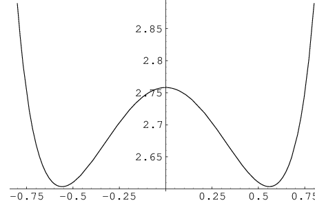
In Fig. 1 we show the dependence of $K_{SV}(c)$.

A contribution from emission of a hard photon in collinear kinematics can be obtained using the method of quasi-real electrons [3]. For this purpose we introduce some numerically small angle $\theta_{0}$ and consider emission of an additional hard photon inside the cones $\theta<\theta_{0}$ along the electron and positron direction of motion. The chiral amplitude method cannot be applied to this kinematical region since the chirality is not a good quantum number for collinear kinematics. We distinguish emission along the initial electron $\theta<\theta_{0}$, where $\theta$ is the angle between 3-momenta of electron (we choose this direction as the $z$ axis) and photon with energy $\omega$

and emission along positron: $\pi-\theta<\theta_{0}$ with numerically small value of $\theta_{0}<<1$

with $L_{\theta}=L+\log(\frac{\theta_{0}}{2})^{2},\theta_{0}\ll 1$ and the expressions for the shifted cross sections are given in (5).

The contribution of the kinematics when all three hard photons are emitted in so called non-collinear kinematics (all three photons are emitted outside cones $\theta<\theta_{0},\quad\pi-\theta\ll\theta_{0}$) can be obtained using the chiral amplitude method [4]

with¹¹ 1 In paper[6] (1997) in the right hand sides of 4.3 and 4.6 the multipliers $\frac{1}{3!}$ and $\frac{1}{2}$ were lost.

and

$c_{1},c_{2},c_{3}$ are the cosines of the photon emission angles to the initial electron 3-momentum. Using the on mass shell conditions and the conservation of 4-momentum law we can put the expression for $d\Phi$ in one of the equivalent forms

and similar ones obtained from this expression by permutations of the indices. Here $dO_{1},dO_{3}$ are the angular phase volumes and $c_{13}=1-2(1-\nu_{2})/(\nu_{1}\nu_{3})$ is the cosine of the angle between the photons 1, 3 directions.

It can be seen that the dependence on the auxiliary parameters $(\Delta E/E)$ and $\theta_{0}$ will be cancelled in the expression of $K^{hard}$ defined as

Here the symbol $\Theta$ means restrictions on the manifold of integration variables $d\Phi$. They are: all three energy fractions must exceed $\Delta E/E$ (hardness condition) and, besides, the conservation law restrict $\vec{k}_{1}+\vec{k}_{2}+\vec{k}_{3}=0$. In particular,

The noncollinear kinematics conditions must also be put on: $\theta_{0}<\theta_{i}<\pi-\theta_{0}$. Moreover, the experimental cuts connected with detection of the final photons can be included in this set of cuts. These conditions depend on experimental set-ups. It is them reason why we do not consider it in numerical estimations here.

Terms containing ”large logarithm” $L$ can be put in the form

with

which is the kernel of the evolution equation of twist-2 operators [2]. The parameter $x$ can be interpreted as the energy function of electron considered as a parton in the initial electron. In such a way, one can obtain the general form of cross section in the form of cross-section of Drell-Yan process given above (see (4)) with

In [5] another form of $D(x,L)$ was found

In Appendix A we give the expression for the virtual correction to the two quantum annihilation cross section in the high energy large scattering angle limit. Its analytic form is given above (see (15)). The result of tabulation of $K_{SV}$ is given in the table. The total value of $K_{2}$ is $K_{2}=K_{VS}+K^{hard}$.

For completeness, we also give the cross section of $3\gamma$ annihilation. In [7] it was shown that in the leading logarithmical approximation it has the form (4) with replacement $d\sigma_{B}$ by $d\sigma^{hard}$ (see(12)). The value of K-factor ($K=K_{3}$) is rather a cumbersome function of kinematical invariants. Rather realistic estimation for it can be obtained by using the averaging procedure: replacing the ratio of amplitudes of nonleading contributions to an amplitude of leading ones and expressing them in terms of cross sections. The cross section of $3\gamma$ annihilation through the light-by-light mechanism turns out to be dominant among nonleading terms. This contribution does not contain large logarithms $L$.

This cross section was calculated in [8]

In [4], the so called ”total” cross section of the process $e^{+}e^{-}\to 3\gamma$ in the lowest order of PT was obtained. The detection energy threshold of final photons $\frac{2\omega_{i}}{E}=\nu_{i}>\eta$. Was implied moreover $\psi_{0},(\cos\psi_{0}=z\sim 1)$-is the minimal angle between the plane of photons momentum and beam axis was fixed. It has a form:

The Explicit form of functions $\varphi_{1}(z),\varphi_{2}(z)$ is given in Appendix B.

Keeping in mind the smooth behavior of the non-leading contributions in the kinematic region of large-angle photon emission, we estimate the $K_{3}$ using the ”total cross section” approximation:

Numerical estimation for $z=0.3$ and $\eta=0.05$ leads to $1+(\alpha/\pi)K_{3}\approx 1.01$.

One of us (EAK) acknowledges the support of to the Institute of Physics, SAS and INTAS Grant 05-1000008-8328. The work also was partly supported by the Slovak Grant Agency for Sciences VEGA, Grant No. 2/7116/27. We are grateful to Yu. M. Bystritskii for interest in this paper, and G.V. Fedotovich for useful critical remarks.

In the case under consideration the result of calculation of the lowest order correction due to virtual photons has a form:

expression form is rather cumbersome in general case([1]) $G(\chi_{1},\chi_{2})$ has a form: In the large angle kinematic it is

Substituting here $\chi_{1}=(s/2)(1+c),\chi_{2}=(s/2)(1-c)$ and taking into account soft photon emission contribution we arrive after some algebra at expression (8).

The explicite forms of $\varphi_{1},\varphi_{2}$ are

References

• [1] L. Brown and R. Feynman, Phys. Rev.85 (1952),231;
J. Harris and L. Brown Phys. Rev. 105 (1957),1656;
F. A. Berends and R. Gastmans, Nucl.phys. B61(1973),414.
• [2] G. Altarelli, G. Parisi Nucl. Phys. B126(1977),298;
L. Lipatov, Yad. Fiz. 20(1974),181.
• [3] V. Baier, V. Fadin and V. Khoze, Nucl. Phys. B65(1973),381.
• [4] S. Eidelman, E. Kuraev and V. Panin, Nucl. Phys. B148(1979),245.
B. V. Geshkenbein and M. V. Terentjev, Yad. Fiz. 8 (1968),550.
• [5] E. Kuraev and V. Fadin, Sov. J. Nucl. Phys. 41(1985),466.
• [6] A. B. Arbuzov, et.al. JHEP 9710 (1997) 006
• [7] E. A. Kuraev and Z. K. Silagadze, Phys. Atom. Nucl. 58 (1995) 1741 [Yad. Fiz. 58 (1995) 1843].
• [8] V. Baier, E. Kuraev and V. Fadin Yad. Fiz. 31(1980),700.