Dynamics of dark energy with a coupling to dark matter
Abstract
Dark energy and dark matter are the dominant sources in the evolution of the late universe. They are currently only indirectly detected via their gravitational effects, and there could be a coupling between them without violating observational constraints. We investigate the background dynamics when dark energy is modelled as exponential quintessence, and is coupled to dark matter via simple models of energy exchange. We introduce a new form of dark sector coupling, which leads to a more complicated dynamical phase space and has a better physical motivation than previous mathematically similar couplings.
I Introduction
Observations are providing increasingly compelling evidence that the expansion of the Universe is accelerating, driven by “dark energy” (see e.g. [1] for recent results). The simplest model of dark energy is a cosmological constant , representing the vacuum energy density, and this model provides a very good fit to a range of independent observations. However, there is no satisfactory theoretical explanation for the very small value of . Furthermore, the model suffers from a fine-tuning, or “coincidence”, problem – why is the dark matter density comparable to the vacuum energy density now, given that their time evolution is so different?
If the dark energy evolves with time, this may alleviate the coincidence problem. The simplest models of evolving dark energy are light scalar fields, known as “quintessence”. If the quintessence is coupled to the dark matter, then this may be able to account for the similar energy densities in the dark sector today. A decisive way of achieving similar energy densities is if the coupling leads to an accelerated scaling attractor solution, with
| (1) |
In this case, the coincidence problem is reduced to a simple choice of parameters to match to observations. Since the accelerated scaling solution is an attractor, no fine-tuning of initial conditions is needed. However, the dynamics that produces such scaling in the dark sector may have other undesirable consequences.
Here we study quintessence with an exponential potential,
| (2) |
where is dimensionless and . The dynamics of a universe with exponential quintessence and an uncoupled perfect fluid have been studied, and these models do not admit late-time accelerated scaling attractors that satisfy Eq. (1) [2]. When we introduce a coupling between the quintessence and dark matter, accelerated scaling attractors are possible [3, 4]. However, in some models, this is achieved at the expense of introducing other problems which can rule out the model [5].
A general coupling between a quintessence field and dark matter (with density ) may be described in the background by the balance equations,
| (3) | |||||
| (4) |
Here is the rate of energy density exchange in the dark sector, and
| (5) |
The dark energy equation of state parameter is
| (6) |
The modified Klein-Gordon equation follows from Eq. (4):
| (7) |
When we include baryons () and radiation (), the remaining evolution equations are
| (8) | |||||
| (9) | |||||
| (10) |
subject to the Friedman constraint,
| (11) |
We can define effective equation of state parameters for the dark sector, which describe the equivalent uncoupled model in the background: , . By Eqs. (3) and (4),
| (12) |
It follows that
When it is possible that (see [7] for specific examples). This means that the coupled quintessence behaves like a “phantom” uncoupled model – but without any negative kinetic energies.
Equations (3)–(10) are an autonomous system of the form
| (19) |
and the critical points satisfy . In order to study the stability of the critical points, we expand about them, , and Eq. (19) yields
| (20) |
Here as , and
| (21) |
is a constant non-singular matrix, whose eigenvalues encode the behaviour of the dynamical system near the critical point.
If a component of can be written as a fraction , then a critical point requires the vanishing of the numerator, . If the denominator also vanishes at the critical point, , then care is needed in obtaining the eigenvalues of the linearized system (19). Strictly speaking, the fraction may not be well defined. However, it is still possible to obtain analytical results via analysis of the behavior of the eigenvalues of in the limit .
II Models of the dark sector coupling
There is as yet no basis in fundamental theory for a specific coupling in the dark sector, and therefore any coupling model will necessarily be phenomenological, although some models will have a more physical justification than others. Various models of energy exchange have been considered. Some of these are simple functional ansatzes, such as . However these models are incomplete: they cannot be thoroughly tested against observations, since one has no idea what the perturbation of should be.
A satisfactory model requires at least that should be expressed in terms of the energy densities and other covariant quantities. Two simple examples represent two of the main types of model:
| (I) | (22) | ||||
| (II) | (23) |
where and are dimensionless constants whose sign determines the direction of energy transfer, according to Eq. (5):
| (24) |
For model (II), the case corresponds to the decay of dark matter into dark energy, with decay rate .
Coupling (I) may be motivated within the context of scalar-tensor theories [3, 4, 6]. Generalizations of this model allow for and more general forms of (see, e.g., Refs. [7, 8]). Couplings which generalize or are closely related to model (II) have been considered as well, see, e.g., Refs. [9] for and Ref. [10] for .
For simplicity, we neglect the baryons (which are not coupled to dark energy), and we neglect radiation (since we are mainly interested in the late universe). The Friedman constraint (11) becomes
| (25) |
and the total equation of state parameter is given by
| (26) |
The condition for acceleration is .
We introduce the same dimensionless variables as in the uncoupled case [2], where
| (27) |
and Eq. (25) implies that
| (28) |
In the new variables, the equation of state parameters are
| (29) |
At a critical point , it follows that
| (30) |
The Hubble evolution equation may be written as
| (31) |
The energy balance equations (3) and (4) for coupling models (I) and (II) are independent of when expressed in the variables and , where . Thus Eq. (31) is not needed for these coupling models, and the phase space is two-dimensional space.
Coupling Model (I):
The autonomous system is
| (32) | |||||
| (33) |
where a prime denotes . The critical points and the conditions for stability, acceleration () and physical existence, are summarized in Table 1, where for convenience we have introduced the parameters
| (34) |
Table 1 combines all the possible cases ( and negative and positive), and recovers the particular results of previous work [4, 11, 6] in the case of pressure-free matter ().
| Point | Stable? | Acceleration? | Existence? | ||||
| A | 1 | 0 | and | 1 | 1 | no | all |
| B | 0 | and | 1 | 1 | no | all | |
| C | and | 1 | |||||
| ; | |||||||
| D | and: | and | |||||
| or | |||||||
| E | 0 | stable when it exists | no | ||||
| and is hyperbolic |
The complicated stability conditions for critical point D were confirmed numerically, and the results are shown in Fig. 1. This point is an accelerated scaling solution that allows for Eq. (1) to be satisfied, i.e.,
| (35) |
Acceleration requires . This includes positive and negative (provided that is accordingly restricted), but in the uncoupled case, , acceleration is not possible for the scaling solution.
Point E is also a scaling solution, but it is always decelerating.

Coupling Model (II):
The autonomous system of equations in this case is
| (36) | |||||
| (37) |
We summarize the critical points and their properties in Table 2. Our results cover all signs of and and agree with previous results [11] for . Two additional critical points, E and F, occur for .
| Point | Stable? | Acceleration? | Existence? | ||||
| A | 1 | 0 | and | 1 | 1 | no | all |
| B | -1 | 0 | and | 1 | 1 | no | all |
| C | and | 1 | |||||
| D | see Fig. 2 | and | |||||
| E | and | no | |||||
| F | and | no | |||||

Furthermore, we have performed numerical integrations to probe the complicated stability conditions for the critical point D. The results are summarized in Fig. 2. Point D again allows for accelerated scaling solutions that satisfy Eq. (1), provided that . In the uncoupled case , and for positive (decay of dark matter into dark energy), acceleration is not possible for D.
Points E and F are also scaling solutions, but they are always decelerating.
III Coupling model (III):
Coupling model (I) was introduced via scalar-tensor theory [3, 4], and was shown to produce accelerated scaling solutions. Although model (I) has a clear physical motivation, it is ruled out by observations [5]: the accelerated scaling attractor is not connected to a matter era where structure grows in the standard way. Indeed, generalizations of (I) with face the same problem [5].
Coupling model (II) is not based on a physical model of dark sector interactions, but is designed for mathematical simplicity. This model and its simple generalization [9], , are specifically designed to produce an accelerated scaling attractor. Model (II) and its generalization evade the problems that model (I) has with a non-standard matter era [12]. These models are useful for phenomenology, but it is difficult to see how they can emerge from a physical description of dark sector interactions. The rate of transfer, , is determined by the expansion rate of the universe – rather than by purely local quantities associated with particle/ field interactions.
In order to avoid this problem, we follow [13] and replace the non-local transfer rate of model (II) by a local rate ,
| (38) |
where we assume that is constant. This form of is
used
in other contexts. When , the same is used in:
(1) a simple model to describe the decay of dark matter into
radiation [14],
(2) a simple model for the decay of
a curvaton field into radiation [15],
(3) a special case of a model in which superheavy dark matter
particles decay to a quintessence scalar
field [16].
When , the energy transfer in Eq. (38) corresponds to the decay of dark matter into dark energy. Models with decay of dark matter to dark energy allow for the possibility that there is no dark energy field in the very early universe, and that dark energy “condenses” as a result of the slow decay of dark matter. Coupling model (III) includes also the case which describes a transfer of energy from dark energy to dark matter:
| (39) |
It turns out that the resulting evolution equations do not allow a two-dimensional representation of this model, since we cannot eliminate from the energy balance equations (3) and (4), using the variables . Equation (31) must therefore be incorporated into the dynamical system. We do this via a new variable , chosen so as to maintain compactness of the phase space:
| (40) |
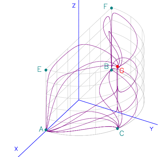
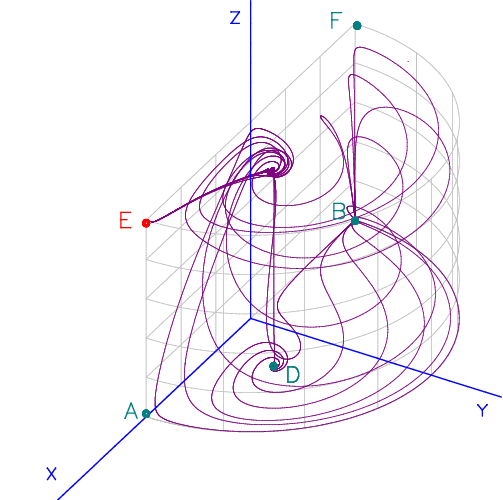
Thus , and the compactified phase space now corresponds to a cylinder of unit height and radius. We also re-scale to a dimensionless coupling constant:
| (41) |
Then we arrive at the autonomous system
| (42) | |||||
| (43) | |||||
| (44) |
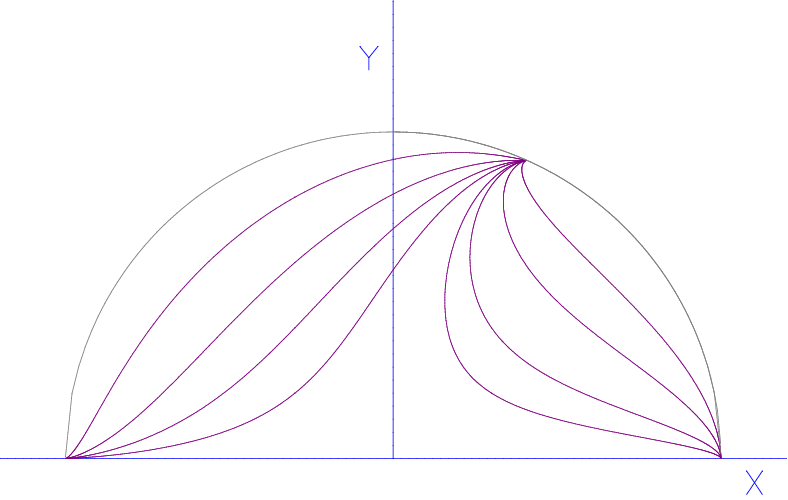
Since the system is invariant under , the phase space may be reduced to a unit semi-cylinder.
In order to determine the critical points and their stability, we need to deal with the singularities at in Eq. (42). We rewrite the right-hand side of Eq. (42) with a common denominator, in the form . Of the total of seven points that give and , three of them also give . The points A, B, C, D of Table 3 are the critical points for the early universe, since corresponds to . These are the same critical points as occur in the uncoupled case. The new points E, F, G with are late-universe versions of A, B, C ().
Our results are summarized in Table 3. The stability behaviour shown in Table 3 is based on the eigenvalues of the linearized matrix, Eq. (21), which are shown in Table 4. In fact, only the signs of the real and imaginary parts of the eigenvalues are of importance. Therefore, we consider the eigenvalue simply as a positive/ negative eigenvalue.
| Point | Stable? | Acceleration? | Existence? | |||||
| A | 1 | 0 | 0 | saddle node for | 1 | 1 | no | all |
| unstable node for | ||||||||
| B | -1 | 0 | 0 | unstable node for | 1 | 1 | no | all |
| saddle node for | ||||||||
| C | 0 | saddle node | 1 | |||||
| D | 0 | saddle node for | no | |||||
| saddle focus for | ||||||||
| E | 1 | 0 | 1 | stable node for and | 1 | 1 | no | all |
| saddle node for and | ||||||||
| saddle node for and all | ||||||||
| F | -1 | 0 | 1 | saddle node for and all | 1 | 1 | no | all |
| stable node for and | ||||||||
| saddle node for and | ||||||||
| G | 1 | stable node for | 1 | |||||
| saddle node for |
| Point | Eigenvalues | |||
|---|---|---|---|---|
| A | 1 | 0 | 0 | |
| B | -1 | 0 | 0 | |
| C | 0 | |||
| D | 0 | |||
| E | 1 | 0 | 1 | |
| F | -1 | 0 | 1 | |
| G | 1 |
Apart from the extra dimension in its phase space, model (III) differs from models (I) and (II) in one key aspect:
- •
In models (I) and (II), the new behaviour introduced by coupling includes the possibility of an accelerated scaling solution (point D), characterized by Eq. (1). In model (III), no such accelerated scaling solution is possible. Instead, the accelerated attractor introduced by the coupling is point G, which has
(45) This is the same qualitative behaviour as the standard CDM model.
Our analytical results are supported by numerical integrations, giving a consistent picture of the dynamical properties of coupling model (III). Illustrative examples are shown in Figs. 3 and 4. Trajectories for are shown in Fig. 3, showing the critical point G in Table 3. In Fig. 4, we plot trajectories when , and the stable node that corresponds to the point E is apparent.
An interesting feature of the trajectories before reaching the global attractor (E, F or G, depending on the values of and ), is that they seem to be focused near a point that is vertically above the early-universe critical point D, and close to the surface. Analysis of the system shows that the coordinates and derivatives of this (non-critical) point are
| (46) | |||
| (47) |
In the limit of zero coupling, we have , and this point collapses to the critical point D. The deviation of this point from being critical is . When is small, as in the plots, this explains the presence of focusing of trajectories in the numerics.
IV Conclusions
We considered the background dynamics of a universe dominated by dark energy (in the form of exponential quintessence) and cold dark matter, where there is energy exchange in the dark sector, as in Eqs. (3) and (4),
For the previously introduced forms of , given in Eqs. (22) and (23),
the phase space remains two-dimensional, as in the uncoupled case . We found the properties of the critical points for all signs of . The results are summarized in Tables 1 and 2, and slightly extend previous work [4, 6, 11] in the case of pressure-free matter (). In both models, critical point D is the cosmologically relevant point, because for nonzero coupling it includes accelerated scaling attractor solutions,
The stability behaviour of critical point D was investigated numerically, and is shown in Fig. 1 for model (I) and Fig. 2 for model (II).
Our main results are for a new coupling model [13], defined in Eq. (38),
This has a similar form to model (II), but is more physical since the transfer rate is determined only by local properties of the dark sector interaction at each event, and is not dependent on the universal expansion rate. When , this new model has the same form as simple models for the decay of dark matter particles to radiation [14], or to quintessence [16], and for the decay of the curvaton field into radiation [15].
Model (III) requires a three-dimensional phase space, since the Hubble rate cannot be eliminated from the equations for . This makes the dynamics more complicated than for models (I) and (II). In particular, a new set of late-time critical points arises in (III), and considerable analytical effort is required to identify these points and determine their stability properties. Our results are summarized in Tables 3 and 4. We performed numerical integrations of the dynamical system in order to confirm the analytical results, and examples of these integrations are shown in Figs. 3 and 4.
The cosmologically relevant critical point is G, which allows for an accelerated critical solution (when ). However, this is not a scaling solution, since
which is similar to the asymptotic behaviour of the standard CDM model. This accelerated critical solution is an attractor when , i.e., for the case when dark matter is decaying to dark energy. Note that in model (II), the decaying dark matter case, , does not lead to any accelerated attractor (see Table II). Model (III) with produces an interesting class of models where dark matter decays to dark energy – so that the primordial universe may have no dark energy – and where this decay eventually leads to dark energy dominance, independent of initial conditions (since there is an attractor). Although such models do not solve the coincidence problem in the standard way, they may provide a new approach to the broader problem of explaining why dark energy dominates over dark matter only late in the universe’s evolution.
The background dynamics for coupling model (III) show new features not present in the previously investigated models (I) and (II). In order to confront this model with observations, the cosmological perturbations with a dark sector coupling of form (III) need to be investigated (see Ref. [13]).
Acknowledgements:
We thank Luis Ureña-López, Elisabetta Majerotto, Luca Parisi, Israel Quirós, Jussi
Väliviita and Shinji Tsujikawa for useful discussions. GCC is supported by the
Programme Alban, the European Union Programme of High Level
Scholarships for Latin America, scholarship no. E06D103604MX and
the Mexican National Council for Science and Technology, CONACYT,
scholarship no. 192680. RL is supported by the University of the
Basque Country through research grant GIU06/37, and by the Spanish
Ministry of Education and Culture through research grants
FIS2004-01626 and FIS2004-0374-E. The work of RM is supported by
STFC.
References
- [1]
D. N. Spergel et al. [WMAP Collaboration],
Astrophys. J. Suppl. 170, 377 (2007)
[arXiv:astro-ph/0603449];
M. Tegmark et al., Phys. Rev. D 74, 123507 (2006) [arXiv:astro-ph/0608632];
W. J. Percival, S. Cole, D. J. Eisenstein, R. C. Nichol, J. A. Peacock, A. C. Pope and A. S. Szalay, Mon. Not. Roy. Astron. Soc. 381, 1053 (2007) [arXiv:0705.3323 [astro-ph]]. - [2] E. J. Copeland, A. R. Liddle and D. Wands, Phys. Rev. D 57, 4686 (1998) [arXiv:gr-qc/9711068].
- [3] C. Wetterich, Astron. Astrophys. 301, 321 (1995) [arXiv:hep-th/9408025].
- [4] L. Amendola, Phys. Rev. D 60, 043501 (1999) [arXiv:astro-ph/9904120].
- [5] L. Amendola, M. Quartin, S. Tsujikawa and I. Waga, Phys. Rev. D 74, 023525 (2006) [arXiv:astro-ph/0605488].
- [6] D. J. Holden and D. Wands, Phys. Rev. D 61, 043506 (2000) [arXiv:gr-qc/9908026].
- [7]
G. Huey and B. D. Wandelt,
Phys. Rev. D 74, 023519 (2006)
[arXiv:astro-ph/0407196];
S. Das, P. S. Corasaniti and J. Khoury, Phys. Rev. D 73, 083509 (2006) [arXiv:astro-ph/0510628]. - [8]
R. Bean and J. Magueijo,
Phys. Lett. B 517, 177 (2001)
[arXiv:astro-ph/0007199];
R. Bean, Phys. Rev. D 64, 123516 (2001) [arXiv:astro-ph/0104464];
L. Amendola, C. Quercellini, D. Tocchini-Valentini and A. Pasqui, Astrophys. J. 583, L53 (2003) [arXiv:astro-ph/0205097];
D. Comelli, M. Pietroni and A. Riotto, Phys. Lett. B 571, 115 (2003) [arXiv:hep-ph/0302080];
G. R. Farrar and P. J. E. Peebles, Astrophys. J. 604, 1 (2004) [arXiv:astro-ph/0307316];
M. B. Hoffman, arXiv:astro-ph/0307350;
U. Franca and R. Rosenfeld, Phys. Rev. D 69, 063517 (2004) [arXiv:astro-ph/0308149];
R. Fardon, A. E. Nelson and N. Weiner, JCAP 0410, 005 (2004) [arXiv:astro-ph/0309800];
F. Vernizzi, Phys. Rev. D 69, 083526 (2004) [arXiv:astro-ph/0311167];
X. J. Bi, P. h. Gu, X. l. Wang and X. m. Zhang, Phys. Rev. D 69, 113007 (2004) [arXiv:hep-ph/0311022];
S. Lee, K. A. Olive and M. Pospelov, Phys. Rev. D 70, 083503 (2004) [arXiv:astro-ph/0406039];
A. W. Brookfield, C. van de Bruck, D. F. Mota and D. Tocchini-Valentini, Phys. Rev. Lett. 96, 061301 (2006) [arXiv:astro-ph/0503349];
T. Koivisto, Phys. Rev. D 72, 043516 (2005) [arXiv:astro-ph/0504571];
H. Wei and R. G. Cai, Phys. Rev. D 72, 123507 (2005) [arXiv:astro-ph/0509328];
R. Mainini and S. Bonometto, JCAP 0706, 020 (2007) [arXiv:astro-ph/0703303];
A. Fuzfa and J. M. Alimi, Phys. Rev. D 75 (2007) 123007 [arXiv:astro-ph/0702478];
R. Bean, E. E. Flanagan and M. Trodden, arXiv:0709.1124 [astro-ph]; ibid.
arXiv:0709.1128 [astro-ph];
T. Gonzalez and I. Quiros, arXiv:0707.2089 [gr-qc]. - [9]
W. Zimdahl and D. Pavon,
Phys. Lett. B 521, 133 (2001)
[arXiv:astro-ph/0105479];
L. P. Chimento, A. S. Jakubi, D. Pavon and W. Zimdahl, Phys. Rev. D 67, 083513 (2003) [arXiv:astro-ph/0303145];
J. D. Barrow and T. Clifton, Phys. Rev. D 73 (2006) 103520 [arXiv:gr-qc/0604063];
H. M. Sadjadi and M. Alimohammadi, Phys. Rev. D 74, 103007 (2006) [arXiv:gr-qc/0610080]. - [10] Z. K. Guo, N. Ohta and S. Tsujikawa, Phys. Rev. D 76 (2007) 023508 [arXiv:astro-ph/0702015].
- [11] A. P. Billyard and A. A. Coley, Phys. Rev. D 61, 083503 (2000) [arXiv:astro-ph/9908224].
- [12] G. Olivares, F. Atrio-Barandela and D. Pavon, arXiv:0706.3860 [astro-ph].
- [13] J. Valiviita, E. Majerotto and R. Maartens, in preparation.
- [14]
R. Cen,
Astrophys. J. 546, L77 (2001)
[arXiv:astro-ph/0005206];
M. Oguri, K. Takahashi, H. Ohno and K. Kotake, Astrophys. J. 597, 645 (2003) [arXiv:astro-ph/0306020]. - [15] K. A. Malik, D. Wands and C. Ungarelli, Phys. Rev. D 67, 063516 (2003) [arXiv:astro-ph/0211602].
- [16] H. Ziaeepour, Phys. Rev. D 69, 063512 (2004) [arXiv:astro-ph/0308515].