Nonequilibrium transport in mesoscopic multi-terminal SNS Josephson junctions
Abstract
We report the results of several nonequilibrium experiments performed on superconducting/normal/superconducting (S/N/S) Josephson junctions containing either one or two extra terminals that connect to normal reservoirs. Currents injected into the junctions from the normal reservoirs induce changes in the electron energy distribution function, which can change the properties of the junction. A simple experiment performed on a 3-terminal sample demonstrates that quasiparticle current and supercurrent can coexist in the normal region of the S/N/S junction. When larger voltages are applied to the normal reservoir, the sign of the current-phase relation of the junction can be reversed, creating a “-junction.” We compare quantitatively the maximum critical currents obtained in 4-terminal -junctions when the voltages on the normal reservoirs have the same or opposite sign with respect to the superconductors. We discuss the challenges involved in creating a “Zeeman” -junction with a parallel applied magnetic field and show in detail how the orbital effect suppresses the critical current. Finally, when normal current and supercurrent are simultaneously present in the junction, the distribution function develops a spatially inhomogeneous component that can be interpreted as an effective temperature gradient across the junction, with a sign that is controllable by the supercurrent. Taken as a whole, these experiments illustrate the richness and complexity of S/N/S Josephson junctions in nonequilibrium situations.
pacs
74.50.+r, 73.23.-b, 85.25.Am, 85.25.CpI Introduction
When a superconducting metal (S) and a normal metal (N) are placed in contact with each other, the properties of both metals are modified near the S/N interface. This effect, called the superconducting proximity effect, was widely studied in the 1960’s.[1] Our microscopic understanding of the proximity effect underwent dramatic progress in the 1990’s as a result of new experiments performed on submicron length scales, coupled with theoretical ideas about phase-coherent transport from mesoscopic physics. It is now understood that the conventional proximity effect in S/N systems and the dc Josephson effect in S/N/S junctions arise from the combination of three ingredients: Andreev reflection of electrons into holes (and vice versa) at the S/N interface, quantum phase coherence of electrons and holes, and time-reversal symmetry in the normal metal. Our new understanding of the proximity effect in equilibrium situations and in linear response transport is demonstrated by a wealth of beautiful experiments [2] and is summarized in several theoretical reviews.[3, 4]
In the past several years, research in S/N systems has increasingly focused on nonequilibrium phenomena. Understanding nonequilibrium situations is more difficult than understanding near-equilibrium situations, because the electron energy distribution function in nonequilibrium may be quite different from a Fermi-Dirac function. In such situations, the behavior of a specific sample may depend critically on the rates of electron-electron or electron-phonon scattering. A pioneering work in this area was the demonstration by Baselmans et al.[5] that the current-phase relation of a S/N/S Josephson junction can be reversed, producing a so-called “-junction”. This effect is produced by applying a voltage that suitably modifies the form of the distribution function.
This paper presents results of several experiments performed on S/N/S Josephson junctions with extra leads connecting the N part of the devices to large normal reservoirs. Samples are made from polycrystalline thin films of aluminum (S) and silver (N) deposited by thermal evaporation. Electrical transport is in the diffusive limit – i.e. the electron mean free path is much shorter than all other relevant length scales in the problem, including the sample length and the phase coherence length. In these experiments, the two superconductors are usually at the same potential, referred to as ground. Different voltages are applied to the normal reservoirs, which in most cases cause the distribution function in the structures to deviate strongly from a Fermi-Dirac distribution.
Several of the experiments have been analyzed quantitatively within the framework of the Usadel equations,[6, 4] which are appropriate for S/N samples in the diffusive limit. The equilibrium component of the Usadel equation is a diffusion equation describing pair correlations in N and S. The nonequilibrium, or Keldysh, component consists of two coupled Boltzmann equations for the spectral charge and energy currents. Incorporating inelastic scattering into the Keldysh equations involves inserting the appropriate collision integrals; but this procedure has so far been followed fully in only a few cases. Moreover, the effect of inelastic scattering on the equilibrium component of the Usadel equation or the proximity effect on the collision integrals have never been included self-consistently to our knowledge. More commonly, researchers analyzing nonequilibrium phenomena solve either the Keldysh equation without collision integrals, or the standard Boltzmann equation with collision integrals but without superconducting correlations, depending on which aspect of the problem is more important. At the end of this paper we compare these approaches as applied to the last experiment discussed in the paper.

The paper is organized as follows: Section II describes the sample fabrication and measurement techniques. Section III describes a simple experiment, called the “dangling arm”, involving a 3-terminal S/N/S device with a single extra lead to a normal reservoir. The dangling arm experiment was first reported by Shaikhaidarov et al..[7] We include it here because it provides a clear demonstration of the superposition of quasiparticle current and supercurrent in a S/N/S junction, an essential result for the remainder of the paper. Section IV describes the -junction experiment in 3- and 4-terminal devices. The 4-terminal sample allows a direct comparison of the situations present in the 3-terminal -junction[8] and the original 4-terminal -junction of Baselmans et al.[5] Section V discusses the behavior of the critical supercurrent as a function of magnetic field applied parallel to the plane of the sample, and shows the difficulty involved in trying to achieve a -junction by Zeeman splitting of the conduction electrons.[9, 10] The theoretical calculation relevant to this geometry is given in the appendix. Section VI discusses an experiment in which supercurrent and quasiparticle current are independently controlled in a 3-terminal S/N/S junction, leading to an effective temperature gradient across the junction.[11] The local distribution function is measured by a tunnel probe near one of the S/N interfaces. The discussion provides information that was not included in our previous report on this experiment.[12] Together these experiments demonstrate the richness of phenomena present in S/N/S Josephson junctions under nonequilibrium conditions.
II Experimental Techniques
II.1 Fabrication
All samples in this work were fabricated using e-beam lithography. A bilayer of resist was deposited onto an undoped Si wafer covered only with its native oxide layer. The bilayer was formed by first depositing a copolymer P(MMA/MAA), followed by a second layer of PMMA. The bilayer was exposed by 35-keV electrons and then developed to make a mask for evaporation. With the resist bilayer, it is possible to fabricate undercuts in the mask, allowing angled evaporation techniques to be used.[13] Therefore, multiple layers of different metals (either purity Al or purity Ag) were sequentially deposited without breaking vacuum.
These techniques were used to prepare the sample shown in Fig. 1. To create the tunnel probe (TP), 30 nm of Al was deposited while the sample was tilted 45 degrees, creating an actual thickness of about 21 nm of Al on the surface. Next, a mixture of 90%Ar-10% O2 gas was leaked into the vacuum chamber to a pressure of 60 Torr. After 4 minutes, the chamber was evacuated again, in preparation for the following depositions: For the silver wires; labeled , , and ; 30 nm of Ag was deposited with the plane of the wafer perpendicular to the evaporation source. For the superconducting reservoirs, S1 and S2, the sample was tilted 45 degrees and rotated 180 degrees in order to deposit 90 nm of Al (for a 60 nm thickness). Finally, the sample was rotated another 140 degrees in preparation for a final, thick layer of Ag to be deposited over the normal reservoir, N. The sample in Fig. 6 followed a similar procedure, except foregoing the first Al deposition and oxidation steps.
II.2 Experimental setup
Samples were measured inside the mixing chamber of a top loading dilution refrigerator. All electrical leads to the sample passed through commercial LC -filters at the top of the cryostat and cold RC filters in the cryostat consisting of 2.2 k resistors in series and 1 nF capacitors coupled to ground.
Current-voltage characteristics (I-V curves) were obtained through 4-probe measurements across the sample. The current was swept using a triangle wave and several cycles were collected and averaged together. Measurements of were obtained by adding a slow ( mHz) triangle wave pattern to the sine output of a lock-in amplifier. The lock-in amplifier was operated at low frequencies (less than 100 Hz) to allow for extrapolation of the system response to zero frequency. Both the in-phase and out-of-phase components of the signal were recorded and utilized in the analysis.
III Dangling Arm Experiment
The dangling arm experiment was first proposed in the Ph.D. thesis of S. Gueron,[14] although a related geometry was discussed by Volkov two years earlier.[15] The experiment is performed on a 3-terminal S/N/S Josephson junction sample similar to the one shown in Fig. 1, in which the tunnel probe in the lower left was unused. We label the three terminals of the sample S1, S2, and N, and the resistances of the three arms , , and . (We neglect for the moment the variation of these resistances due to proximity effect.) One measures the resistance from N to S1, while leaving S2 open (dangling). Naively, one might expect the measured resistance between N and S1 to be equal to . That result would imply that the current travels directly from N to S1, which in turn implies that S1 and S2 are at different voltages. Given that S1 and S2 are coupled by the Josephson effect, the relative phase between S1 and S2 then accumulates at the Josephson frequency, . If, however, the injected current splits into a piece through and a piece through , such that , then S1 and S2 will be at the same potential. To avoid having a net current flowing into the dangling arm, the sample must then provide a supercurrent from S2 to S1 that exactly cancels the quasiparticle current . In this scenario, and are effectively acting in parallel, and the measured resistance will be .

Figure 2 shows the 2-terminal curve taken at mK from a sample similar to the one shown in Fig. 1, with nominal resistance values , , and . The inset shows vs. , providing a clearer view of the effective resistance. Either plot shows that the resistance is about 20.7 when the applied current is less than about 0.94 A. This resistance is very close to the nominal value of . When the current exceeds 0.94 A, the resistance increases to the value 24.6 , which is very close to . (Resistance differences less than an Ohm are attributed to the finite size of the “T-junction” in the middle of the sample.) These data confirm the idea outlined in the previous paragraph, that supercurrent and quasiparticle current can coexist in the normal region of a S/N/S Josephson junction.
The transition at where the resistance increases to occurs when the supercurrent across the S/N/S Josephson junction exceeds the S/N/S critical current, . However, since only the fraction of the injected current must be cancelled by the supercurrent, one should expect that . The data in Figure 3 show that this expectation is fulfilled at relatively high temperatures, but that at lower temperature falls well below this value.
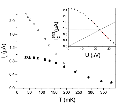
Two reasons for the small values of at low temperature were given by Shaikhaidarov et al..[7] Those authors solved the Usadel equation analytically in the limit where the S/N interfaces have high resistance (poor transparency), so that proximity effects are small and the Usadel equation can be linearized. They pointed out that is suppressed below its equilibrium value due to the applied voltage at N, a result we will reinforce below. They also argued that the phase-dependence of the resistances , , and due to proximity effect causes the measured value of to be smaller than the nominal value .
We believe that the effect related to the phase dependence of the resistances is small and the relative decrease in at low temperature is due predominantly to the decrease in as a function of . This effect is demonstrated graphically in the inset to Fig. 3. There the critical current of the Josephson junction, , multiplied by the constant ratio , is plotted as a function of the voltage applied to the normal reservoir. As can be seen in the inset, decreases rapidly as a function of . The straight line through the origin in the inset represents the current injected into the sample from the N reservoir, , where the resistances are evaluated at phase difference between S1 and S2. The intersection of the two curves shows the value of the dangling arm critical current (ordinate) at the critical voltage (abscissa). The figure demonstrates the large reduction in S/N/S critical current due to the applied voltage , which explains why is much smaller than at low temperature. At high temperatures , the relative reduction is less significant due to two reasons: First, increasing the temperature decreases the critical current , and thereby also . Moreover, to observe a sizable reduction in , has to exceed .
IV S/N/S nonequilibrium -Junction
IV.1 Three-terminal -junction
Figure 3 shows, not surprisingly, that the critical current of an S/N/S Josephson junction decreases when quasiparticle current is injected into the junction from a normal reservoir. Indeed, if the only effect of the injected current were to heat the electrons in the junction, then one would expect the critical current to continue decreasing monotonically as a function of the applied voltage .[16] That this is not the case represents a major discovery in nonequilibrium superconductivity by Baselmans et al.[5] in 2000. Those authors showed that first decreases as a function of , but then increases again at higher . The explanation[17, 18] for this counter-intuitive result consists of two pieces. First, one can view the supercurrent in the sample as arising from the continuous spectrum of Andreev bound states in the normal metal,[19, 20] which carry supercurrent in either direction, depending on their energy. Second, in the presence of the applied voltage the electron distribution function in the junction is not a hot Fermi-Dirac distribution, but is closer to a two-step distribution - as long as the short sample length does not allow electron thermalization within the sample.[21] The two-step distribution function preferentially populates the minority of Andreev bound states that carry supercurrent in the direction opposite to the majority, hence it reverses the current-phase relation in the junction.[17, 18] Such a Josephson junction is called a “-junction”, because the energy-phase and current-phase relations are shifted by relative to those of standard Josephson junctions.
The original -junction experiment of Baselmans et al. was performed in a 4-terminal sample, where voltages of opposite sign were applied to the two normal reservoirs. Later, Huang et al.[8] demonstrated that a -junction can also be obtained in a 3-terminal geometry with a single normal reservoir, a result predicted by van Wees et al.[22] 10 years earlier.

Figure 4a shows results of a 3-terminal -junction experiment performed on a sample similar to the one in Fig. 1, where the tunnel probe in the lower left portion of the figure is not used. We measure the curve of the S/N/S Josephson junction using a 4-probe current-bias measurement, while a dc voltage is simultaneously applied to the normal reservoir via a battery-powered floating circuit. Figure 4a shows a series of curves at different values of the voltage applied to the normal reservoir. Figure 4b shows the critical current vs. . Notice that initially decreases with an increasing , as shown in the inset to Fig. 3. But as increases further, reaches a minimum value (indistinguishable from zero in this experiment[23]) at V, then grows again to reach a second maximum at V. The minimum in separates the standard Josephson junction behavior at low values of from the -junction behavior at higher . If instead of plotting the critical current (which is by definition a positive quantity) one were to plot the supercurrent at a fixed phase difference across the junction then the graph would show a smooth curve passing through zero at , reaching a local minimum at V and gradually returning to zero at large .

IV.2 Comparison of four-terminal -junctions with symmetric and antisymmetric bias
The physical explanation of the -junction in the 3-terminal sample is the same as in the 4-terminal sample, with the differences arising only from the distribution functions. Figure 5 shows a schematic drawing of the distribution function along a path from a reservoir N to S for both 4-terminal and 3-terminal samples for , assuming weak electron-electron interactions in the N wire, and neglecting the proximity corrections. Notice in figures c and d that consists of a double-step function, the step height within the energy range to changing with the location along the wire. As we will show in the next section, the even (in energy) part of has no effect on the magnitude of the supercurrent (in the absence of electron-electron interactions), suggesting that the voltage-dependent critical current, , would be identical in 3-terminal and 4-terminal samples with identical dimensions and resistances. However, there are three reasons why this is not quite true: First, Joule heating is more prevalent in the 4-terminal device, which rounds the distribution functions more than in the 3-terminal device. Second, the spectral supercurrent density, , evaluated at the junction point will be slightly smaller in the 4-terminal sample than in the 3-terminal sample due to the presence of the additional arm connecting the sample to a normal reservoir.[20] Finally, will be slightly more rounded in the 4-terminal sample due to the increased phase space available for electron-electron interactions. Roughly speaking, the rate of e-e interactions at a given energy is proportional to , which is maximized when . Each of these effects serve to increase in the 3-terminal geometry relative to the 4-terminal geometry.
It is not practical to compare critical currents from two different samples, since they will never have identical dimensions nor electrical resistances. Instead, it was proposed in Ref. 8 to compare the critical currents in a single 4-terminal sample under conditions of symmetric and antisymmetric voltage bias of the two normal reservoirs. Figure 6 shows the sample we fabricated for this experiment, with the superconductive reservoirs labeled S1 and S2 and the normal reservoirs labeled N1 and N2. By applying a positive potential to N1 and a negative potential to N2, one reproduces the experiment performed by Baselmans et al. We call this situation antisymmetric bias, since the two applied voltages differ by a negative sign. In this case the quasiparticle current overlaps with the supercurrent only at the crossing point of the sample where the electrostatic potential is equal to zero. In contrast, applying the identical voltage on both N1 and N2 (with ground defined at one of the superconducting electrodes), called symmetric bias, will produce a situation mimicking that in the 3-terminal experiment of Huang et al.[8] Notice that by mimicking a 3-terminal sample with a 4-terminal sample, geometrical differences between the two experiments are eliminated, so any observed difference in the critical currents will be due either to e-e interactions or to Joule heating.

The preceding description of symmetric and antisymmetric biases holds strictly only if the resistances of the two lower arms are identical. Otherwise, application of antisymmetric bias will result in a nonzero potential at the cross and some quasiparticle current will flow into the superconducting reservoirs. In that case, f(E) will take a form intermediate between those depicted in Figures 5c and d, which decreases the measurement contrast between the two biases. In our experiments we took care to measure the resistances of all the arms and to ensure that the voltages at the two normal reservoirs were indeed equal (for symmetric bias) or opposite (for antisymmetric bias).

Figures 7a and 7b show curves measured across the S/N/S junction at mK, for several different values of . Curves with increasing values of are offset upward for clarity. Figure 7a shows the data for antisymmetric bias while Fig. 7b shows symmetric bias. The data follow the same trend observed in Fig. 4, namely, the critical current first decreases with increasing , then increases again before finally disappearing altogether. Figure 8b shows this critical supercurrent as a function of . In this figure we have plotted the critical current as negative in the range of voltages after disappears initially, to signify that the junction is in the -state as discussed earlier.

The transition from the 0-state to the -state can be confirmed directly by experiment,[5] without recourse to the theoretical explanation. The resistances of the Ag arms of the sample vary with the phase due to the proximity effect.[24] The phase , in turn, varies between as a function of the supercurrent passing between S1 and S2; hence, one observes a variation of the resistances as a function of . This effect is shown in Figs. 7c and d, in which the resistances between N1 and N2 (N1 and S2) were measured versus for the antisymmetric and symmetric bias configurations, respectively. Each curve in the lower two figures has the same value of as the corresponding curve in the upper figures. One can see that proximity effect induces a local minimum in the resistance at when the junction is in the 0-state, because that is where . In contrast, the resistance exhibits a local maximum in the resistance at when the junction is in the -state, because . Interestingly, the top curve in Fig. 7d shows that at large enough values of , the system returns to the 0-state since the resistance again shows a local minimum at . This high- transition from the -state back to the 0-state was not visible in the S/N/S curves.
Figure 8 shows the behavior vs. at two different temperatures. The squares represent antisymmetric bias while triangles represent symmetric bias. Both bias configurations appear similar in that the samples cross to the -state at nearly the same value of . It should be noted, however, that the maximum -current is larger for symmetric bias than for antisymmetric bias. That result is consistent with the qualitative arguments made above. In the next section we present a quantitative analysis of the results.
IV.3 Calculation of the Critical Current in an S/N/S Josephson Junction
The amount of supercurrent passing through an S/N/S Josephson junction may be calculated by [17]
| (1a) | |||||
| (1b) | |||||
where and are the conductivity and cross-sectional area of the normal metal, respectively. is the distribution function within the normal wire, and is the antisymmetric component of with respect to the potential of the superconductors. The spectral supercurrent density, , is an odd function of energy, and describes the amount of supercurrent at a given energy travelling between superconductors with relative phase difference . In the samples considered in the present work, it is generally sufficient to calculate the supercurrent using the the distribution function at the crossing point of the wires.
To determine , we solve the Usadel equation numerically using the known physical dimensions and electrical resistances of the various wire segments of the sample. We then look for consistency with the measured temperature dependence of the equilibrium critical current, shown in Fig. 9. The used to fit these data, evaluated at , is shown in the inset of Fig. 9. Since the length of the junction is much longer than the superconducting coherence length of the S electrodes for all the samples studied in this work, the damped oscillations in occur on an energy scale given by the Thouless energy, , where is the diffusion constant in the wire. characterizes the temperature scale over which the equilibrium critical current drops to zero, and also determines the voltage scale needed to create a nonequilibrium -junction. The transition from the 0-state to the -state occurs at . The fit shown in Fig. 9 was obtained with eV.

Next we calculate in the nonequilibrium situation with antisymmetric bias, i.e. with voltages and applied to reservoirs N1 and N2. Because we are interested in the distribution function far from the superconducting reservoirs, we consider using the Boltzmann equation. Let us first ignore the supercurrent and proximity effects, although inclusion of those effects will be discussed in detail in Sec. VI. In a reservoir at voltage , is a Fermi-Dirac distribution displaced by energy , . In the experiment with antisymmetric bias, we then have at reservoir N1 and at reservoir N2. If we neglect inelastic electron scattering, then in the middle of the wire (at the intersection of the cross) has the double-step shape:
| (2) |
In fact, the odd part of is the same everywhere in the Ag wire:
| (3) |
This conclusion holds also in the presence of the proximity effect. At energies , the even part, , varies linearly with distance between the two reservoirs (the lower two arms of the sample), but is zero everywhere along the direct path connecting the two superconductors (in the ideal case where the resistances of the two lower arms are equal).
To calculate in the experiment with symmetric bias, we need the boundary conditions at the interfaces between the normal wires and the superconducting reservoirs. For energies below the superconducting gap, , these conditions are and , where . These boundary conditions assume high-transparency interfaces, no charge imbalance in the superconductors, and no heat transport into the superconductors.[25] (Note that is discontinuous at the N-S interface for energies below the gap, and returns to the standard form in the S electrodes.) The solution for at the N/S interface is identical to Eq. (2), but the symmetric component is nonzero elsewhere in the wire. Notice that the odd component of the distribution function, , is identical in the two cases everywhere in the sample. The proximity effect induces a small feature in discussed in Sec. VI, but it is zero at the crossing point in the middle of the sample.
Calculation of in the realistic situation requires consideration of electron-electron interactions in the Ag wire. (The electron-phonon interaction, in contrast, is much weaker, and need be considered only in the massive normal reservoirs. See the discussion below.) To incorporate electron-electron interactions, we solved the Boltzmann equation in the wire numerically, following previous work by Pierre.[26, 27] The results of this numerical calculation of in the situations with either symmetric or antisymmetric bias were extremely similar. Indeed, the slight additional rounding of in the antisymmetric case could not account for the differences observed in the experiment, shown in Fig. 8.
To account for the difference in the observed between the two experiments, we next considered the effect of Joule heating on the temperatures of the normal reservoirs. (Due to Andreev reflection at the N/S interfaces, there is no heat transport into the superconducting reservoirs.) Although we intentionally fabricated the normal reservoirs much thicker than the wires, this was not enough to eliminate the effects of Joule heating altogether. The heat current in a reservoir at a distance from the juncture with the wire is given by:
| (4) |
where is the total power dissipated in the wire, and nm are the conductivity and the thickness of the reservoir, respectively, and V2/K2 is the Lorenz number. (We neglect the small additional Joule heat generated in the reservoirs themselves.) The spreading angle if we consider the combination of the two normal reservoirs shown in Fig. 6.
Using (4) as a boundary condition, one can find an effective temperature at the wire-reservoir interface equal to [28]
| (5) |
The temperature far away in the normal reservoir is assumed to be , the bath temperature. The factor is given by [29]
| (6) |
where is the sheet resistance of the normal reservoir, the wire width, and is the distance over which the electrons in the reservoir thermalize to the bath temperature via electron-phonon scattering. The parameter varies inversely with the thickness of the metal reservoir and the electrical resistance encountered by the quasiparticle current in the wire. Because the voltage drop in the antisymmetric bias situation occurs entirely between a normal reservoir and the crossing point, the resistance is smaller than in the symmetric bias situation where drops fully from the N reservoirs to the N/S interfaces. The larger current in the former case causes more Joule heating, and hence a larger reservoir temperature. For our sample, the values of needed to fit the data (see solid lines in Figs. 8a and 8b) are and K/mV, respectively, for the symmetric and antisymmetric bias experiments. Their ratio of 1.2 matches the ratio calculated from the sample parameters. Their magnitudes, however, are nearly three times larger than what we calculate based on the total reservoir thickness. The experiment seems to suggest that heat was trapped in the 35-nm Al layer at the bottom of the reservoirs, rather than immediately spreading throughout the whole reservoir thickness.[30]
V Application of a Parallel Magnetic Field, and the “Zeeman” -junction
There is a long history of applying magnetic fields perpendicular to the direction of current flow in superconductor/insulator/superconductor (S/I/S) Josephson junctions, to observe the famous Fraunhofer pattern in the critical current. In S/N/S junctions, the Fraunhofer pattern is observed only in wide junctions, whereas narrow junctions exhibit a monotonic decrease of the critical current with field due to the orbital pair-breaking effect.[31]
In this section we discuss the effect of a magnetic field applied parallel, rather than perpendicular, to the current direction. In this geometry there should never be a Fraunhofer pattern. And because the samples are thin films, one expects the orbital pair-breaking effect to be much weaker than for a field applied perpendicular to the plane. In the case of an extremely thin sample the Zeeman (spin) effect should dominate over the orbital effect of the field.
The effect of Zeeman splitting on an S/N/S Josephson junction was studied theoretically in 2000 by Yip[10] and by Heikkilä et al..[9] Their idea is that the electronic structure of a normal metal in a large applied magnetic field resembles that of a weak ferromagnet, in that the up and down spin bands are displaced by the Zeeman energy. They also showed how the Zeeman-split junction behaves analogously to the nonequilibrium S/N/S junction, with the Zeeman energy playing the role of the voltage in Eqs. (1b) and (3). Josephson junctions made with real ferromagnetic materials (S/F/S junctions) are the subject of intense current interest, as they can also show -junction behavior.[32] Unlike the -junctions discussed earlier in this paper, however, the -junctions in S/F/S systems occur in equilibrium. They appear only in particular ranges of the F-layer thickness, due to spatial oscillations in the superconducting pair correlations induced in the F metal near the F-S interface by proximity effect. Those oscillations, in turn, arise from the different Fermi wavevectors of the spin-up and spin-down electrons in the F metal. In diffusive S/F/S junctions, the sign of the coupling between the two superconductors oscillates over a distance scale , where is the diffusion constant and is the exchange energy in the ferromagnet. In the standard elemental ferromagnets, is large ( meV), hence is extremely short – on the order of 1 nm. Control of sample thickness uniformity at this scale is difficult, hence several groups have used dilute ferromagnetic alloys, with reduced values of , to increase . The advantage of the “Zeeman” -junction is that it is fully tunable by the field. The disadvantage is that the sample must be thin enough to minimize the effects of orbital pair-breaking in both the superconducting electrodes and in the normal part of the junction.

Figure 10 shows a plot of vs. in an S/N/S sample whose normal part had length m, width nm and thickness nm. The critical current decreases monotonically to zero, over a field scale of T. This result might appear surprising at first glance: At a field T, the magnetic flux enclosed in the cross-section of the wire perpendicular to the field is only Tm, where is the superconducting flux quantum. Furthermore, separate tests of the Al banks confirm that they remain superconducting to fields of order 0.85 T.
A quantitative understanding of the data in Figure 10 can be obtained from a solution to the Usadel equation. The analysis discussed in Appendix A shows how a parallel magnetic field can be absorbed into a spin-flip rate in the equations. This allows us to apply the scaling for the zero-temperature supercurrent of an S/N/S junction found in Ref. 33 and find
| (7) | ||||
| (8) |
Our numerical calculations confirm that this scaling also applies in our multi-probe experimental geometry. This prediction is in a good agreement with the experiment, as seen in Fig. 10.
In the limit , the characteristic field scale varies as , rather than the more intuitive result we might expect based on the cross-sectional area of the wire perpendicular to the field. The physical explanation for this result was given by Scheer et al.[34] in a paper discussing universal conductance fluctuations as a function of parallel field in normal metal wires. As an electron travels down the length of a long diffusive wire, its trajectory circles the cross-section of the wire many times – on order . Because diffusive motion can be either clockwise or counterclockwise as seen looking down the wire, the standard deviation in net flux and accumulated phase between different trajectories is approximately proportional to , which gives the scaling for dephasing.
It is instructive to ask what constraints on the sample geometry would have to be met to enable observation of the Zeeman -junction. We estimate the Thouless energy of the sample discussed in Fig. 10 to be eV both from the temperature dependence of (not shown), and from the voltage-induced transition to the -state at V (inset to Fig. 10). According to theory, the Zeeman -junction should occur when ,[10, 9], or T. Attempts to make thinner samples in order to increase the field scale in Eq. (7) were unsuccessful, due to the tendency of very thin Ag films to ball up. According to the theory, much thinner films, with of the order of , will be required to enable observation of the Zeeman -junction.
VI Engineering the Distribution Function
The discussion in Section IV.B. implied that the 3-terminal and 4-terminal -junctions are similar, with only minor differences due to a slight decrease in the phase space available for electron-electron interactions in the 3-terminal case. But that oversimplified discussion misses some important physics. Heikkilä et al.[11] showed that the superposition of quasiparticle current and supercurrent in the horizontal wire in the 3-terminal sample induces a change in the distribution function at energies of order . The new feature is antisymmetric in space and energy (see Fig. 16 for the theoretical prediction and our experimental results which follow each other nicely), and can be interpreted as a gradient in the effective electron temperature across the S/N/S junction. For this reason, the result was dubbed a “Peltier-like effect.” Although a tiny cooling effect does occur, observing it in a real electron temperature would require a slightly modified experimental setup.[35] In the present case, one should view this effect mostly as a redistribution of the Joule heat generated in the sample by the applied bias .
In Sec. IV.3 it was discussed how the distribution functions behave in the absence of proximity effects and supercurrent. Including these effects, but ignoring inelastic scattering, results in the kinetic equations:[36]
| (9a) | |||
| (9b) |
where and are the spectral charge and energy currents, respectively. The energy-dependent coefficients , , , and can be calculated from the Usadel equation [6, 36], and vary with the superconducting phase difference between S1 and S2. In general, these equations must be solved numerically; however, they can be solved analytically by ignoring the energy dependence in and and neglecting the terms. One can show that, in the presence of both the applied voltage and a nonzero supercurrent between S1 and S2, along the horizontal wire connecting the two superconductors contains a spatially antisymmetric contribution proportional to . In the exact numerical solution to Eqs. (9b), the feature is distorted due to the rapid evolution of the diffusion coefficients and near the N/S interfaces.[11]
The antisymmetric feature in can be measured by performing tunneling spectroscopy with a local superconducting tunnel probe, which has been demonstrated by Pothier et al.[21] to reveal detailed information about in a metal under nonequilibrium conditions. In our case, the local probe must be placed close to the N/S interface where the predicted feature in has its maximum amplitude. This location introduces a new difficulty in our experiment because the density of states (DOS) of the Ag wire near the N/S interface is strongly modified by proximity effect. Hence we must first determine the modified DOS at equilibrium before we measure under nonequilibrium conditions.
The current-voltage characteristic of the probe tunnel junction is
| (10) | |||||
where is the normal state tunnel resistance, and are the normalized densities of states, and and are the electron energy distribution functions on the Ag and Al sides of the tunnel junction, respectively. The function characterizes the probability for an electron to lose energy to the resistive environment while tunneling across the oxide barrier, an effect known as “dynamical Coulomb blockade”.[37] was determined from equilibrium measurements at high magnetic field, where superconductivity is completely suppressed. Details of the fitting procedure used to extract were reported earlier. [12]

Quantitative analysis of our tunneling data requires an accurate determination of the superconducting gap, , hence we fabricated a second S/I/N tunnel junction simultaneously with the sample, but placed about m away from it, and with the N side of the junction far from any superconductor. Tunneling spectroscopy measurements on this reference junction, shown in Fig. 11(a), were fit to Eq. (10) with independent of energy and with the standard BCS form for , to provide an accurate determination of .
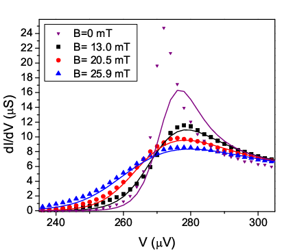
Several of our tunnel junctions exhibited sharp anomalies in the conductance data for voltages close to the superconducting gap; however, these features disappeared with the application of a small magnetic field of mT.[38] Figure 12 shows data for one particular tunnel probe for different magnetic field strengths. Along with each data set are fits using the standard BCS form for with a small depairing parameter proportional to , which has been shown to account well for applied magnetic fields.[39] Adding this term effectively rounds the DOS in the superconductor. Following the notation of Ref. 39 we determined a depairing parameter of for mT and a superconducting gap in the Al of eV. This rather large value for was consistent across samples and is believed to be due to oxygen incorporated into thin, thermally-evaporated Al films.[40, 41]
With the form for confirmed, it is possible to analyze the data for the sample tunnel probe, which is in close proximity to superconducting reservoirs. Figure 11(b) shows the for this probe with an external field of 12.5 mT applied. The differences between the data from tunnel probes nearby or far away from superconducting reservoirs arise from changes in the DOS of the normal wire due to the proximity effect. Rather than a flat DOS used to fit the data in Fig. 11(a), the DOS in the Ag wire near the superconducting reservoirs is modified as shown by the squares in Fig. 11(d). This shape was obtained by deconvolving the data.
Also shown in Fig. 11(d) is the density of states of the Ag wire determined from a numerical calculation of the Usadel equation (solid line). This calculation requires knowledge of the sample dimensions, the gap in the superconducting reservoirs, and the Thouless energy. The sample dimensions were obtained from scanning electron micrographs, such as the one shown in Fig. 1. The gap in the superconducting reservoirs was found to be eV. This value of is much smaller than the value in the Al tunnel probe because the reservoirs are much thicker than the tunnel probes (and presumably contain much less oxygen), and because they are close to a normal metal-superconductor bilayer. Finally, the Thouless energy was determined by fitting the critical current vs. temperature data as discussed in Section IV.3. The value of was then refined through self-consistent calculations involving both the finite probe size and the position dependent order parameter in the superconducting reservoirs.

When supercurrent flows through the S/N/S junction, the phase difference of the reservoirs, , changes . For this reason, data were also taken with supercurrent flowing across the S/N/S junction. The resulting fits of for and , which are identical to each other, are shown in Fig. 13 along with one for . It is noteworthy that the change of shape (more narrow at low energies, broader at intermediate ones) is qualitatively consistent with theoretical calculations shown in the inset.

It was anticipated that applying a voltage to the normal lead would not alter so that it would be possible to deconvolve the distribution function, , for the system out of equilibrium. Figure 14 shows that this assumption does not hold, as the best fits for applied voltages and are poor. Only by using an altered was it possible to fit the data in Fig. 14.
Changes in with increasing are probably due to a slight suppression of the gap in the superconducting electrodes, which are adjacent to superconductor/normal-metal bilayers. To estimate how changes, we used two different forms for the distribution function . First, we computed from Eqs. (9b)(a) and (b), which include proximity effects due to the nearby superconducting reservoirs, but neglect inelastic scattering. Second, we solved the diffusive Boltzmann equation with collision integrals for electron-electron scattering, while neglecting superconducting correlations. The two forms for the distribution functions are shown in Figs. 15(a) and (b) for two different values of U: and . Using those distribution functions, new densities of states were obtained by deconvolution of the data and are shown as the symbols in Figs. 15(c) and (d). Notice that the two different forms of the distribution function yield similar results for . Figures 15(c) and (d) also show obtained from equilibrium data, as the solid lines. However, the resulting does not obey the sum rule
that should be valid in all situations. We do not know what causes this discrepancy.

Fortunately it is possible to extract information about using a method that is relatively insensitive to the exact form of , by taking advantage of a near-symmetry of the data with respect to the direction of . The data shown in Fig. 13 confirm our expectation that , a symmetry that also holds approximately for . Hence, one can analyze the difference between two data sets with opposite directions of the supercurrent, , which will depend on the differences in the distribution functions, . The effect of analyzing the data with the wrong DOS for the Ag is greatly reduced in this case. The feature we seek in is predicted to be odd in , hence it should be the only contribution to . Figure 16(a) shows with V and , which exhibits the predicted feature that is antisymmetric in energy. The solid lines are the numerical solution to Eqs. (9b), with the parameters and obtained from the previous fits, with no additional fit parameters. The computed theory curves agree well with the experimental data.
A further test of the robustness of the experimental results is to compare the measured form of when the signs of both and are reversed, i.e. . The results of this second measurement are shown superimposed on the first in Fig. 16(a). The agreement between the two data sets is excellent.

Interestingly, applying a voltage V brings this sample into its -state. Figure 16(b) shows data for V and . Compared to Fig. 16(a), the sign of the low-energy feature in is reversed, demonstrating that the phase difference , rather than the supercurrent, determines the sign of the new feature in .
The results of Fig. 16 indicate that the supercurrent has a large effect on the electron energy distribution function inside the normal metal. Such a mechanism has been utilized to explain [36] the large thermopower measured in Andreev interferometers [42] — systems with two normal-metal and two superconducting contacts. Our results confirm this mechanism and point out to new phenomena dependent on it, such as the large Peltier effect [35]: in linear response to the quasiparticle current (voltage), the supercurrent-induced change translates into a change of the electron temperature and the sign of this change (heating or cooling) depends on the relative sign of the supercurrent compared to the sign of the quasiparticle current. One can hence cool part of the structure by simultaneously applying a quasiparticle current and a supercurrent.
VII Conclusions
Superconductor/normal metal hybrid systems exhibit a wealth of fascinating behaviors, starting with the proximity and Josephson effects. Driven out of equilibrium, the possibilities increase, from the non-equilibrium -junction to the supercurrent-induced modification of discussed in the final section of this paper. All of these observations can be interpreted with two main concepts: the spectrum of the supercurrent and the electron distribution function . The latter can be tuned by applying voltages or changing the temperature — the previous for example by applying a magnetic field. In Secs. III, IV and VI we showed in different schemes how the nonequilibrium changes the observed supercurrent and how the supercurrent affects . In Sec. V we discuss the modifications in due to a magnetic field and the resulting changes in the supercurrent. To our knowledge, the effect of a parallel magnetic field on the S/N/S critical current had not been explored in detail before.
As discussed in Refs. 9, 10, the Zeeman effect due to a magnetic field will cause analogous changes in the supercurrent as the nonequilibrium population of the supercurrent carrying states. This exact analogy is distorted on one hand due to the inelastic scattering changing the nonequilibrium distribution function, and on the other hand the orbital effect arising from the magnetic field. It remains an experimental challenge to show this analogy and combine the two effects in the case when the Zeeman effect dominates over the orbital effect. As we discuss in Sec. V, the latter would require constructing extremely thin junctions.
Recently there has been intense interest in the limit where a Josephson junction behaves as a coherent quantum system with one degree of freedom.[43] There is hope that Josephson junctions will someday provide the building blocks for a quantum computer. In the meantime, we hope to have demonstrated that even in the classical regime, the Josephson junction is full of surprising new possibilities.
While preparing this manuscript, we learned about recent related works[31] where the magnetic field dependence of the S/N/S supercurrent was also studied.
Acknowledgements: We thank H. Pothier, D. Esteve, and S. Yip for many valuable discussions. This work was supported by NSF grants DMR-0104178 and 0405238, by the Keck Microfabrication Facility supported by NSF DMR-9809688, and by the Academy of Finland.
Appendix A Usadel equation and the magnetic field
The Usadel equation in a magnetic field can be written as follows, making use of the -parameterization , of the quasiclassical Green’s functions: [6, 4, 10, 9]
| (11) | |||
| (12) |
Here, is the diffusion constant, the vector potential, the spin-flip rate, the gauge-invariant superfluid velocity and the Zeeman energy. The equation is to be solved separately for both spin configurations , assuming spin-independent material parameters. The spin-averaged spectral supercurrent is obtained from the solutions and can be used to calculate the observable supercurrent under various conditions. Below, we consider these equations in a wire that has an uniform cross-section , and assume the boundary conditions
| (13) | ||||||||
| (14) |
where is the boundary of . These imply that we neglect details of the current distribution near the terminal–wire contact.
When a magnetic field is applied to a wire, in addition to the Zeeman splitting, the field induces circulating components to the supercurrent flowing in the wire (see Fig. 17). These currents contribute to decoherence, for example reducing the magnitude of the critical current, and in the general case also prevent reducing Eqs. (11) to one-dimensional equations in the direction parallel to the wire. For thin wires, however, the additional decoherence can be simply absorbed to the spin-flip parameter in the one-dimensional Usadel equation and the vector potential can otherwise be neglected. [33, 44, 39, 45] Below, we show how this conclusion can be reached for an arbitrary orientation of the magnetic field, and that the results are consistent with the discussion in Section V.
Reducing Eq. (11) to a one-dimensional equation is possible when the transverse dimensions of the wire satisfy , where is the distance between the superconducting contacts and a magnetic length scale. This is because varies on the length scales of and when considering energies relevant for the supercurrent. For perpendicular fields it is also possible to directly choose a proper London gauge where varies slowly in the transverse direction and .
Since for , in the experimentally interesting situation we have . To handle the details of the problem in this case, we apply perturbation theory in the parameter . We choose a coordinate system such that is the coordinate parallel to the wire and and correspond to transverse directions, and fix a convenient gauge in which the vector potential is independent of . Finally, we rewrite Eqs. (11) in the dimensionless variables , , , and substitute in the regular series expansion , .
Requiring the equations corresponding to orders , and of expansion to be separately satisfied, we first find that the variables , and are independent of and . We also find that the first-order response is given by
| (15) |
Here, is the boundary of the cross-section of the wire, its outward normal vector, and the operator consists of the transverse components of the gradient. This -independent result applies in the central parts of the wire, away from boundary layers near the ends of the wire. Finally, after averaging the equations of order across the cross section of the wire, we arrive at the result
| (16) | |||
| (17) | |||
| (18) |
This shows how the effective spin-flip parameter is modified by the applied field .
The additional decoherence (18) depends on the direction of the field and the cross section of the wire. For a wire with a circular cross section of radius , we note that Eq. (15) has the exact solution . This results to
| (19) |
For wires with a rectangular cross section, we cannot solve Eq. (15) analytically. However, a variational solution is still possible: we can expand in polynomials of , to orders and project Eq. (15) onto this function basis. From this procedure, we find
| (20) | |||
| (21) | |||
| (22) |
where and are the width and thickness of the wire. For orders we obtain instead
| (23) |
Approximations using higher-order basis produce only slight improvements in accuracy to .

We now note that the contribution of the magnetic field to the decoherence rate is of the form for all directions of the field, where is proportional to some transverse dimension of the wire. Comparing this to the energy scale of the one-dimensional Usadel equation (16), we find a dimensionless parameter that determines how much the magnetic field suppresses coherence. Here, the flux corresponds to an area , which is in agreement with the discussion in Section V.
Finally, note that above we neglected the screening of the magnetic field by the induced supercurrents. However, this should not be important in the experimental case, as the Josephson screening length is larger than the width of the junction, and the aluminum terminals are sufficiently thin as to produce only small screening.
References
- [1] P.G. de Gennes, Rev. Mod. Phys. 36, 225 (1964).
- [2] B. Pannetier and H. Courtois, J. Low Temp. Phys. 118, 599 (2000).
- [3] C.J. Lambert and R. Raimondi, J. Phys.:Condens. Matter 10, 901 (1998).
- [4] W. Belzig, F.K. Wilhelm, C. Bruder, G. Schön, and A.D Zaikin, Superlattices and Microstructures, 25, 1251, (1999).
- [5] J.J.A. Baselmans, A.F. Morpurgo, B.J. van Wees, T.M. Klapwijk, Nature 397, 43 (1999).
- [6] K.D. Usadel, Phys. Rev. Lett. 25, 507 (1970).
- [7] R. Shaikhaidarov, A.F. Volkov, H. Takayanagi, V.T. Petrashov, and P. Delsing, Phys. Rev. B 62 R14649 (2000).
- [8] J. Huang, F. Pierre, T.T. Heikkilä, F.K. Wilhelm, and N.O. Birge, Phys. Rev. B 66, 020507(R) (2002).
- [9] T.T. Heikkilä, F.K. Wilhelm, and G. Schön, Europhys. Lett. 51, 434 (2000).
- [10] S.K. Yip, Phys. Rev. B 62, R6127 (2000).
- [11] T.T. Heikkilä, T. Vänskä, and F.K. Wilhelm, Phys. Rev. B 67, 100502(R) (2003). Note that in this reference there is a sign error in the coefficient, which increases the amplitude of the change .
- [12] M.S. Crosser, P. Virtanen, T.T. Heikkilä, and N.O. Birge, Phys. Rev. Lett. 96, 167004 (2006).
- [13] G.J. Dolan and J.H. Dunsmuir, Physica B 152, 7 (1988).
- [14] S. Gueron, Ph.D. thesis, University Paris VI, France, (1997).
- [15] A.F. Volkov, Phys. Rev. Lett. 74 4730 (1995).
- [16] A.F. Morpurgo, T.M. Klapwijk and B.J. van Wees, Appl. Phys. Lett. 72, 966 (1998).
- [17] S.K. Yip, Phys. Rev. B 58, 5803 (1998).
- [18] F.K. Wilhelm, G. Schön, and A.D. Zaikin, Phys. Rev. Lett. 81, 1682 (1998).
- [19] I.O. Kulik, Sov. Phys. JETP, 30, 944, (1970).
- [20] T.T. Heikkilä, J. Särkkä, F.K. Wilhelm, Phys. Rev. B 66, 184 513 (2002).
- [21] H. Pothier, et al., Phys. Rev. Lett. 79, 3490 (1997).
- [22] B.J. van Wees, K.-M.H. Lenssen, and C.J.P.M. Harmans, Phys. Rev. B 44, 470 (1991).
- [23] J.J.A. Baselmans, T.T. Heikkilä, B.J. van Wees, T.M. Klapwijk, Phys. Rev. Lett. 89, 207002 (2002).
- [24] V. Petrashov, V. Antonov, P. Delsing, and T. Claeson, Phys. Rev. Lett. 74, 5268 (1995).
- [25] A.F. Andreev, Sov. Phys. JETP 19(5), 1228 (1964).
- [26] F. Pierre, Ann. Phys. (Paris) 26, No. 4 (2001), Ch. 3.
- [27] This procedure also neglects the (presumably weak) proximity effect on the kernel of the electron-electron collision integral. These are similar to those in bulk superconductors, see G. M. Eliashberg, Zh. Eksp. Teor. Fiz. 61, 1254 (1971) [Sov. Phys. JETP 34, 668 (1972)].
- [28] K.E. Nagaev, Phys. Rev. B 52, 4740 (1995).
- [29] M. Henny, S. Oberholzer, C. Strunk, and C. Schonenberger, Phys. Rev. B 59, 2871 (1999).
- [30] M.S. Crosser, Ph.D. Thesis, Michigan State University (2005).
- [31] L. Angers, F. Chiodi, J.C. Cuevas, G. Montambaux, M. Ferrier, S. Guéron, H. Bouchiat, [arXiv:0708.0205]; J.C. Cuevas and F.S. Bergeret, Phys. Rev. Lett. 99, 217002 (2007).
- [32] V.V. Ryazanov, V.A. Oboznov, A.Yu. Rusanov, A.V. Veretennikov, A.A. Golubov, and J. Aarts, Phys. Rev. Lett. 86, 2427 (2001).
- [33] J.C. Hammer, J.C. Cuevas, F.S. Bergeret, W. Belzig, Phys. Rev. B 76, 064514 (2007).
- [34] E. Scheer, H.V. Lohneysen, A.D. Mirlin, P. Wölfle, and H. Hein, Phys. Rev. Lett., 78, 3362 (1997).
- [35] P. Virtanen and T.T. Heikkilä, Phys. Rev. B 75, 104517 (2007).
- [36] P. Virtanen and T.T. Heikkilä, J. Low Temp. Phys. 136, 401 (2004), and references therein.
- [37] G.L. Ingold and Y.V. Nazarov, Single Charge tunneling Coulomb Blockade phenomena in Nanostructures, vol. 294 (Plenum Press, London, 1992).
- [38] Similar behavior has been observed by other groups. C.f. p. 40 of F. Pierre, Ann. Phys. (Paris) 26, No. 4, 1 (2001).
- [39] A. Anthore, H. Pothier, and D. Esteve, Phys. Rev. Lett. 90, 127001 (2003).
- [40] R.B. Pettit and J. Silcox, Phys. Rev. B 13, 2865 (1976).
- [41] R.W. Cohen and B. Abeles, Phys. Rev. 168, 444 (1968).
- [42] J. Eom, C.-J. Chien, and V. Chandrasekhar, Phys. Rev. Lett. 81, 437 (1998); A. Parsons, I. A. Sosnin, and V. T. Petrashov, Phys. Rev. B 67, 140502 (R) (2003).
- [43] V. Bouchiat, D. Vion, P. Joyez, D. Esteve, and M.H. Devoret, Physica Scripta T76, 165 (1998).
- [44] W. Belzig, C. Bruder, and G. Schön, Phys. Rev. B 54, 9443 (1996).
- [45] See also Ch. 8 in P.G. deGennes, Superconductivity of Metals and Alloys, (Perseus Books, Massachusetts, 1966).