Scale dependence of alpha effect and turbulent diffusivity
Abstract
Aims. To determine alpha effect and turbulent magnetic diffusivity for mean magnetic fields with profiles of different length scale from simulations of isotropic turbulence, and to relate these results to nonlocal formulations in which alpha and the turbulent magnetic diffusivity correspond to integral kernels.
Methods. A set of evolution equations for magnetic fields is solved which gives the response to imposed test fields, that is, mean magnetic fields with various wavenumbers. Both an imposed fully helical steady flow consisting of a pattern of screw-like motions (Roberts flow) and time-dependent statistically steady isotropic turbulence are considered. In the latter case the aforementioned evolution equations are solved simultaneously with the momentum and continuity equations. The corresponding results for the electromotive force are used to calculate alpha and magnetic diffusivity tensors.
Results. For both the Roberts flow under the second–order correlation approximation and isotropic turbulence alpha and turbulent magnetic diffusivity are largest at large scales and these values diminish toward smaller scales. In both cases the alpha effect and turbulent diffusion kernels are well approximated by exponentials, corresponding to Lorentzian profiles in Fourier space. For isotropic turbulence the turbulent diffusion kernel is half as wide as the alpha effect kernel. For the Roberts flow beyond the second–order correlation approximation the turbulent diffusion kernel becomes negative at large scales.
Key Words.
Magnetohydrodynamics (MHD) – Turbulence1 Introduction
Stars and galaxies harbour magnetic fields whose scales are large compared with the scale of the underlying turbulence. This phenomenon is successfully explained in terms of mean–field dynamo theory discussed in detail in a number of text books and reviews (e.g. Moffatt 1978, Krause & Rädler 1980, Brandenburg & Subramanian 2005a). In this context velocity and magnetic fields are split into large–scale and small–scale components, and , respectively. The crucial quantity of the theory is the mean electromotive force caused by the small–scale fields, . In many representations it is discussed under strongly simplifying assumptions. Often the relationship between the mean electromotive force and the mean magnetic field is tacitly taken as (almost) local and as instantaneous, that is, in a given point in space and time is considered as determined by and its first spatial derivatives in this point only, and the possibility of a small–scale dynamo is ignored. Then the mean electromotive force is given by
| (1) |
with two tensors and . If the turbulence is isotropic the two tensors are isotropic, too, that is and with two scalar coefficients and . Then the expression (1) simplifies to
| (2) |
where we have denoted simply by (so that is times the electric current density, where is the magnetic permeability of free space). The coefficient is, unlike , only non–zero if the turbulence lacks mirror–symmetry. The coefficient is referred to as the turbulent magnetic diffusivity.
In general, the mean electromotive force has the form
| (3) |
where stands for a part of that is independent of , and denotes a convolution in space and time of a kernel with (see, e.g., Krause & Rädler 1980, Rädler 2000, Rädler & Rheinhardt 2007). Due to this convolution, in a given point in space and time depends on in a certain neighborhood of this point, with the exception of future times. This corresponds to a modification of (1) such that also higher spatial and also time derivatives of occur.
In this paper we ignore the possibility of coherent effects resulting from small–scale dynamo action and put therefore equal to zero. For the sake of simplicity we assume further the connection between and to be instantaneous so that the convolution refers to space coordinates only. The memory effect, which we so ignore, has been studied previously by solving an evolution equation for (Blackman & Field 2002).
For homogeneous isotropic turbulence we may then write, analogously to (2),
| (4) |
or, in more explicit form,
| (5) |
with two functions and of that vanish for large . The integration is in general over all –space. Although and as well as and may depend on time the argument is dropped everywhere. For a detailed justification of the relations (4) and (5) we refer to Appendix A. In the limit of a weak dependence of and on space coordinates, i.e. when the variations of and with are small in the range of where and are markedly different from zero, the relations (4) or (5) turn into (2), and we see that and .
At first glance the representations (4) and (5) of look rather different from (3). Considering and carrying out an integration by parts we may however easily rewrite (5) into
| (6) |
with
| (7) |
We further note that due to the symmetry of in only the part of that is symmetric in , i.e. the part that can be described by and its derivatives of even order, contributes to the terms in (5) or in (6) and (7). The symmetry of implies that only the part of antisymmetric in , which corresponds to the derivatives of of odd order, contributes to the terms.
Finally, referring to a Cartesian coordinate system we define mean fields by averaging over all and so that in particular and depend only on and on time. Then (5) turns into
| (8) |
The functions and are just averages of and over all and . They are therefore real and symmetric in . The integration in (8) is in general over all . The remark on the limit of weak dependences of and on space coordinates made above in connection with (4) and (5) applies analogously to (8). We have now and .
Relation (8) can also be brought in a form analogous to (6) and (7),
| (9) |
with
| (10) |
The remarks made under (6) and (7) apply, now due to the symmetries of and in , analogously to (8), (9) and (10).
It is useful to consider in addition to (8) also the corresponding Fourier representation. We define the Fourier transformation in this paper by . Then this representation reads
| (11) |
Both and are real quantities, and they are symmetric in . The limit of weak dependences of and on corresponds here to , and we have and . Detailed analytic expressions for and , or and , can be derived, e.g., from results presented in Krause & Rädler (1980). A numerical determination of quantities corresponding to and has been attempted by Brandenburg & Sokoloff (2002) for shear flow turbulence.
In this paper two specifications of the velocity field will be considered. In the first case is chosen such that it corresponds to a steady Roberts flow, which is periodic in and and independent of . A mean–field theory of a magnetic field in fluid flows of this type, that are of course different from genuine turbulence, has been developed in the context of the Karlsruhe dynamo experiment (Rädler et al. 2002a,b, Rädler & Brandenburg 2003). It turned out that the mean electromotive force , except its component, satisfies relation (2) if any nonlocality in the above sense is ignored (see also Appendix B). Several analytical and numerical results are available for comparison with those of this paper. In the second case is understood as homogeneous, isotropic, statistically steady turbulence, for which the above explanations apply immediately. Employing the method developed by Schrinner et al. (2005, 2007) we will in both cases numerically calculate the functions and as well as and .
2 The method
2.1 A more general view on the problem
We first relax the assumption of isotropic turbulence used in the Sect. 1 (but will later return to it). We remain however with the definition of mean fields by averaging over all and . Then, as already roughly indicated above, and may only depend on and time but , because of , must be independent of . Furthermore all first–order spatial derivatives of can be expressed by the components of , that is, of , where . Instead of (8) we have then
| (12) |
and instead of (11)
| (13) |
with real and , which are even in , and real and , which are even in . A justification of these relations is given in Appendix A. We have further
| (14) |
Since the , as well as the , are of no interest.
In the following we restrict attention to and and assume that is equal to zero. We note that and the contributions of to and are anyway without interest for the mean–field induction equation, which contains only in the form , that is, they do not affect the evolution of . We may formulate the above restriction in a slightly different way by saying that we consider in the following , and as well as , and only for .
As for the mean-field treatment of a Roberts flow depending on and only (and not on ) we refer to the aforementioned studies (Rädler et al. 2002a,b, Rädler & Brandenburg 2003). Following the ideas explained there we may conclude that and with functions and of , and analogously and with functions and of , all for . For obvious reasons the same is true for homogeneous isotropic turbulence.
2.2 Test field method
We calculate the and , or and , numerically by employing the test field method of Schrinner et al. (2005, 2007). It has been originally developed for the calculation of the full and tensors [in the sense of (1)] for convection in a spherical shell. Brandenburg (2005) employed this method to obtain results for stratified shear flow turbulence in a local cartesian domain using the shearing sheet approximation. More recently, Sur et al. (2008) calculated in this way the dependences of and for isotropic turbulence on the magnetic Reynolds number, and Brandenburg et al. (2008) have calculated the magnetic diffusivity tensor for rotating and shear flow turbulence. However, in all these cases no nonlocality in the connection between and has been taken into account.
Following the idea of Schrinner et al. we first derive expressions for with several specific , which we call “test fields". We denote the latter by and define11 1 The notation used here differs slightly from that in Brandenburg et al. (2008), where first test fields were introduced and only later the two versions and are considered.
| (15) |
with any constant and any fixed value of . We then replace and in (12) by and or by and . Denoting the corresponding by or by , respectively, and using (14) we find
| (16) |
for , where
| (17) |
From this we conclude
| (18) |
for .
These relations allow us to calculate the and if the with for both and are known. In preparing the numerical calculation we start from the induction equation. Its uncurled form reads
| (19) |
where is the magnetic vector potential, , and . Here the Weyl gauge of is used. Taking the average of (19) we obtain
| (20) |
From (19) and (20) we conclude
| (21) |
where and .
For the calculation of the we are interested in the which occur in response to the test fields . Specifying (21) in that sense we obtain22 2 In the corresponding expression (27) of Brandenburg (2005) the term is incorrect. This did not affect his results because .
| (22) |
Equations of this type are called “test field equations".
So far no approximation such as the second order correlation approximation (SOCA), also known as first order smoothing approximation, has been made. If we were to make this assumption, terms that are nonlinear in the fluctuations would be neglected and (22) would simplify to
| (23) |
In the following SOCA results will be shown in some cases for comparison only.
In either of the two cases the and are to be calculated from . More details of the numerical calculations of the will be given below in Sect. 2.4.
Returning once more to (18) we note that the depend on both and introduced with the . As a consequence of imperfect simulations of the turbulence they may also depend on the time . The and however should depend on but no longer on and . We remove the latter dependences of our results by averaging and over and . For the Roberts flow there should be no such or dependences.
2.3 Flow fields
2.3.1 Roberts flow
We consider here a special form of a steady flow which, in view of its dynamo action, has already been studied by Roberts (1972). It has no mean part, , and is given by
| (24) |
where
| (25) |
with some constant . The flow is fully helical, . The component form of as defined by (24) and (25) reads
| (26) |
We note that .
2.3.2 Turbulence
Next, we consider isotropic, weakly compressible turbulence and use an isothermal equation of state with constant speed of sound, . Considering first the full velocity field we thus accept the momentum equation in the form
| (27) |
where is a random forcing function consisting of circularly polarized plane waves with positive helicity and random direction, and is the traceless rate of strain tensor. The forcing function is chosen such that the magnitude of the wavevectors, , is in a narrow interval around an average value, which is simply denoted by . The corresponding scale, , is also referred to as the outer scale or the energy-carrying scale of the turbulence. More details concerning the forcing function are given in the appendix of Brandenburg & Subramanian (2005b). With the intention to study the mean electromotive force in the purely kinematic limit the Lorentz force has been ignored.
In addition to the momentum equation we use the continuity equation in the form
| (28) |
In all simulations presented in this paper the strength of the forcing is adjusted such that the flow remains clearly subsonic, that is, the mean Mach number remains below 0.2. Hence for all practical purposes the flow can be considered incompressible (Dobler et al. 2003). In these simulations no mean flow develops, that is , so .
2.4 Simulations
The relevant equations are solved in a computational domain of size using periodic boundary conditions. In the case of the Roberts flow (26) we fix by . Only four of the test field equations (22) (those with , and ) are solved numerically. With turbulence in the kinematic regime the four equations (27) and (28) for and are solved together with four of the test field equations (22) (again with , and ).
Due to the finiteness of the domain in direction and the periodic boundary conditions, quantities like and have to be considered as functions that are periodic in . The Fourier integrals used for representing these quantities, , turn into Fourier series, , where and the summation is over . By this reason only discrete values of , that is , are admissible in (13)–(18). In this framework we may determine the and only for these .
As explained above, the test field procedure yields and not as functions of alone. They may also show some dependence on and . After having averaged over , time averages are then taken over a suitable stretch of the full time series where these averages are approximately steady. We use the time series further to calculate error bars as the maximum departure between these averages and the averages obtained from one of three equally long subsections of the full time series.
In all cases the simulations have been carried out using the Pencil Code33 3 http://www.nordita.org/software/pencil-code which is a high-order finite-difference code (sixth order in space and third order in time) for solving the compressible hydromagnetic equations together with the test field equations. In the case of the Roberts flow, of course, only the test field equations are being solved.
3 Results
3.1 Roberts flow
Let us first recall some findings of earlier work, which are presented, e.g., by Rädler (2002a,b). We use here the definitions
| (29) |
Adapting the results of analytic calculations in the framework of SOCA to the assumptions and notations of this paper (see Appendix B) we have
| (30) |
Moreover, in the general case, also beyond SOCA, it was found that
| (31) |
with a function satisfying and vanishing with growing argument. This function has been calculated numerically and is plotted, e.g., in Rädler et al. (2002a,b).
Fig. 1 shows results for and obtained both by general test field calculations using (22) and under the restriction to SOCA using (23). These results for agree completely with both (30) and (31), and those for agree completely with (30). Unfortunately we have no analytical results for beyond SOCA.
Proceeding now to the and we first note that in SOCA, as shown in Appendix C,
| (32) |
The corresponding and , again in SOCA, read
| (33) |
In Fig. 2 results of test field calculations for the functions and with are shown. We note that becomes negative for small . The same has been observed with another but similar flow of Roberts type (Rädler & Brandenburg 2003). For comparison, SOCA results obtained in two different ways are also shown: those according to the analytic relations (32) and those calculated numerically by the test field method with (23). Both agree very well with each other.
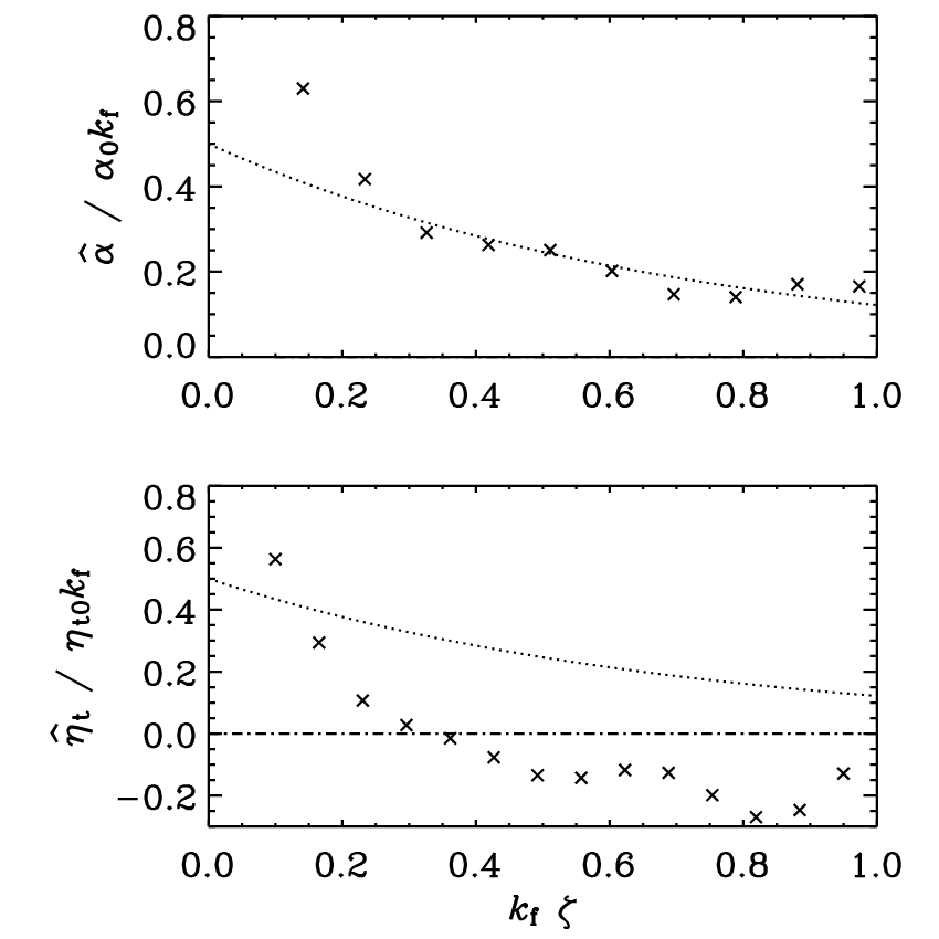
In order to obtain the results for the kernels and we have calculated integrals as in (14) numerically using the data plotted in Fig. 2. The results are represented in Fig. 3. Again, analytical and numerical SOCA results are shown for comparison. Note that the profiles of and beyond SOCA are rather narrow compared with those under SOCA, and that of even more narrow than that of .


3.2 Isotropic turbulence
Results for homogeneous isotropic turbulence have been obtained by solving the hydrodynamic equations (27) and (28) simultaneously with the test field equations (22) in a domain of size . The forcing wavenumbers are fixed by and . Instead of the definitions (29) we use now
| (34) |
Within this framework the dependence of and on has been studied by Sur et al. (2008). They considered two cases, one with and another one with . Remarkably, they found that and approach unity for .
Figure 4 shows results for and with . Both and decrease monotonously with increasing . The two values of for a given but different and are always very close together. The functions and are well represented by Lorentzian fits of the form
| (35) |
In Fig. 5 the kernels and , again with , obtained by calculating numerically integrals as in (14), are depicted. Also shown are the Fourier transforms of the Lorentzian fits,
| (36) |
Evidently, the profile of is half as wide as that of . This corresponds qualitatively to our observation with the Roberts flow beyond SOCA, see the crosses in Fig. 3. There is however no counterpart to the negative values of that occur in the example of the Roberts flow.

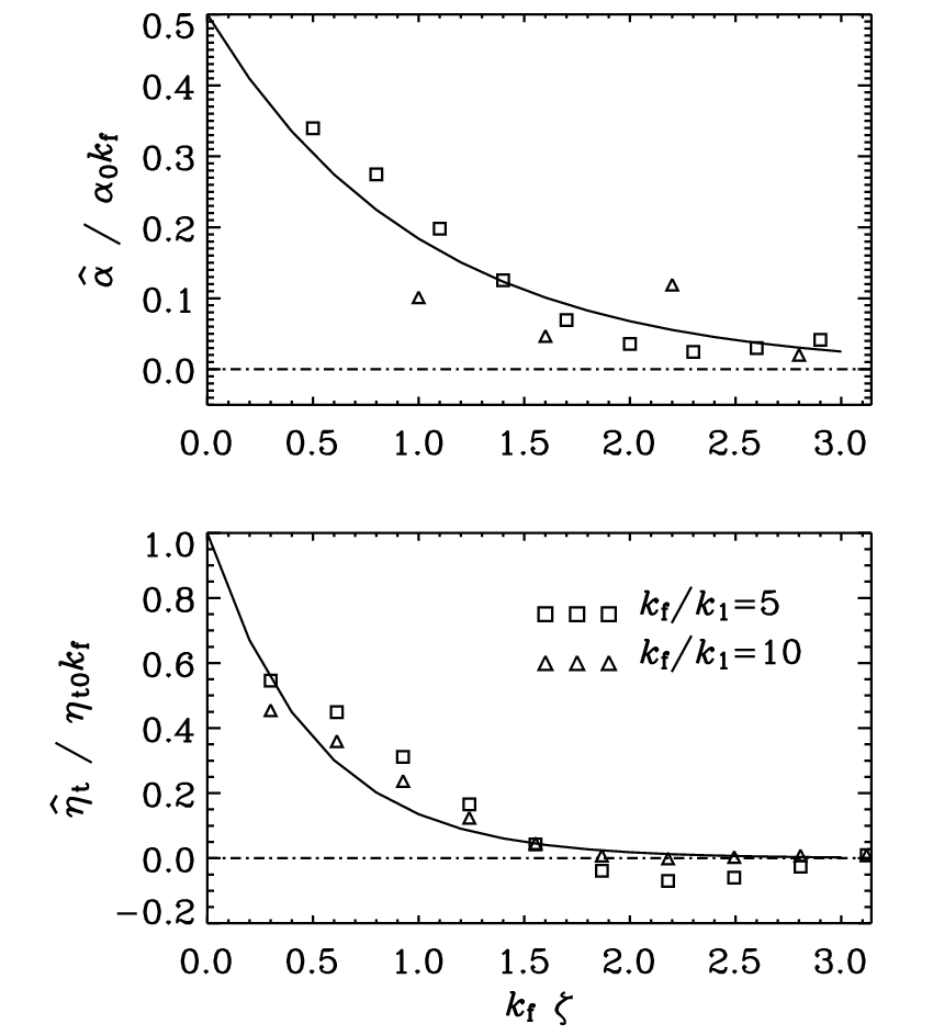
The results presented in Figs 4 and 5 show no noticeable dependences on . Although we have not performed any systematic survey in , we interpret this as an extension of the above–mentioned results of Sur et al. (2008) for and to the integral kernels and . Of course, this should to be checked also with larger values of . Particularly interesting would be a confirmation of different widths of the profiles of and .
4 Discussion
Our results are important for calculating mean–field dynamo models. The mean–field induction equation governing , here defined as average over and , with according to (8), allows solutions of the form , , with the growth rate
| (37) |
A dynamo occurs if is non–negative. Since in all examples considered this occurs with the lower sign, and we focus attention on this case only. In the limit of a local connection between and the and turn into and , respectively.
When using the definitions (29) for the Roberts flow, or (34) for isotropic turbulence, we may write (37) in the form
| (38) |
where for the Roberts case and for the isotropic case. Since and depend only via on we have chosen the arguments .
Consider first the Roberts flow, that is (38) with . Clearly is non–negative in some interval and it takes there a maximum. Dynamos with are impossible. Of course, depends on . With the analytic SOCA results (32) we find that for small and that it grows monotonically with and approaches unity in the limit of large . For small (to which the applicability of SOCA is restricted) a dynamo can work only with small , that is, with scales of the mean magnetic field that are much smaller than the size of a flow cell. Furthermore, never exceeds the corresponding values for vanishing nonlocal effect, which is . In that sense the nonlocal effect favors smaller , that is, larger scales of the mean magnetic field. With the numerical results beyond SOCA represented in Fig. 2, with , we have , again a value smaller than unity. In this case, too, a dynamo does not work with scales of the mean magnetic field smaller than that of a flow cell. There is no crucial impact of the negative values of for on the dynamo.
Proceed now to isotropic turbulence and consider (38) with . Again is non–zero in the interval and it takes there a maximum. Some more details are shown in Fig. 6. With the Lorentzian fits (35) of the results depicted in Fig. 4 we find for (and 0.45 for ). In the limit of vanishing nonlocal effects it turns out that for (and 0.59 for ). We have to conclude that dynamos are only possible if the scale of the mean magnetic field clearly exceeds the outer scale of the turbulence. In addition we see again that the nonlocal effect favors smaller , or larger scales of the mean magnetic field.
These findings may become an important issue especially for nonlinear dynamos or for dynamos with boundaries. Examples of the last kind were studied, e.g., by Brandenburg & Sokoloff (2002) and Brandenburg & Käpylä (2007). In these cases however the underlying turbulence is no longer homogeneous and therefore the kernels and are no longer invariant under translations, that is, depend not only on but also on . The finite widths of the and kernels may be particularly important if there is also shear, because then there can be a travelling dynamo wave that may also show strong gradients in the nonlinear regime (Stix 1972, Brandenburg et al. 2001).


For another illustration of the significance of a finite width of the kernels and we consider a one-dimensional nonlinear mean–field model with periodic boundary conditions. We modify here the model of Brandenburg et al. (2001, Sect. 6), with a dynamo number of 10 (corresponding to 5 times supercritical) and , by introducing the integral kernels (36). Figure 7 shows the components of the mean magnetic field for two different values of and for the conventional case where the kernels are delta–functions. Note that corresponds to the largest scale of the magnetic field compatible with the boundary condition. It turns out that the magnetic field profiles are not drastically altered by the nonlocal effect. Small values of , however, correspond to smoother profiles.
Let us start again from in the form (8), specify there, in view of isotropic turbulence, and according to (36), and represent and by Taylor series with respect to . A straightforward evaluation of the integrals provides us then with
| (39) |
This corresponds to relations of the type (1) or (2), simply generalized by taking into account higher than first–order derivatives of .
The terms with derivatives of in (39) can be interpreted in the sense of hyperdiffusion. While all of them have the same signs in real space, the signs of the corresponding terms in Fourier space alternate, which implies that every second term acts in an anti-diffusive manner. Thus, a truncation of the expansion should only be done such that the last remaining term has an even , as otherwise anti-diffusion would dominate on small length scales and cause to grow beyond any bound.
There are several investigations in various fields in which hyperdiffusion has been considered. In the purely hydrodynamic context, Rüdiger (1982) derived a hyperviscosity term and showed that this improves the representation of the mean velocity profile in turbulent channel flows. In the context of passive scalar diffusion, Miesch et al. (2000) determined the hyperdiffusion coefficients for turbulent convection and found that they scale with like in Eq. (39). We are however not aware of earlier studies differentiating between diffusive and anti-diffusive terms.
We have investigated the nonlocal cases presented in Fig. 7 using truncations of the expansion (39). However, two problems emerged. Firstly, terms with higher derivatives produce Gibbs phenomena, i.e. wiggles in , so the results in Fig. 7 are not well reproduced. Secondly, high–order hyperdiffusion terms tend to give severe constraints on the maximum admissible time step, making this approach computationally less attractive. It appears therefore that a direct evaluation of the convolution terms is most effective.
5 Conclusions
The test field procedure turned out to be a robust method for determining turbulent transport coefficients (see Brandenburg 2005, Sur et al. 2008 and Brandenburg et al. 2008). The present paper shows that this also applies to the Fourier transforms of the integral kernels which occur in the nonlocal connection between mean electromotive force and mean magnetic field, in other words to the more general scale–dependent version of those transport coefficients. For isotropic turbulence the kernels and have a dominant large-scale part and decline monotonously with increasing wavenumbers. This is consistent with earlier findings (cf. Brandenburg & Sokoloff 2002), where however the functional form of the decline remained rather uncertain. Our present results suggest exponential kernels, corresponding to Lorentzian profiles in wavenumber space. The kernel for the turbulent magnetic diffusivity is about half as wide as that for the alpha effect. This result is somewhat unexpected and would be worthwhile to confirm before applying it to more refined mean field models. On the other hand, the effects of nonlocality become really important only when the scale of the magnetic field variations is comparable or smaller than the outer scale of the turbulence.
One of the areas where future research of nonlocal turbulent transport coefficients is warranted is thermal convection. Here the vertical length scale of the turbulent plumes is often comparable to the vertical extent of the domain. Earlier studies by Miesch et al. (2000) on turbulent thermal convection confirmed that the transport of passive scalars is nonlocal, but it is also more advective than diffusive. It may therefore be important to also allow for nonlocality in time. This would make the expansion of passive scalar perturbations more wave-like, as was show by Brandenburg et al. (2004) using forced turbulence simulations.
Acknowledgements.
We acknowledge the allocation of computing resources provided by the Centers for Scientific Computing in Denmark (DCSC), Finland (CSC), and Sweden (PDC). We thank Matthias Rheinhardt for stimulating discussions. A part of the work reported here was done during stays of K.-H. R. and M. S. at NORDITA. They are grateful for NORDITA’s hospitality.Appendix A Justification of equations (5) and (12)
In view of (5) we start with equation (3) for , put , assume that is a purely spatial convolution. Applying then the Fourier transform as defined by we obtain
| (40) |
Since and have to be real we conclude that . Further the assumption of isotropic turbulence requires that is an isotropic tensor. We write therefore
| (41) |
with , and being real functions of . Considering further that and we find
| (42) |
Transforming this in the physical space we obtain immediately (5).
In view of (12) we start again from equation (3) and put but we have to consider now as a convolution with respect to only. Applying a Fourier transformation defined by we obtain a relation analogous to (40),
| (43) |
and may now conclude that . We arrive so at
| (44) |
with real tensors and , which are even in . Combining (43) and (44) and considering that the can be expressed by the (, , ) we may confirm first (13) and so also (12).
Appendix B Mean–field results for the Roberts flow
A mean–field theory of the Roberts dynamo, developed in view of the Karlsruhe dynamo experiment, has been presented, e.g., in papers by Rädler et al. (2002a,b), in the following referred to as R02a and R02b. There a fluid flow like that given by (26) is considered but without coupling of its magnitudes in the –plane and in the –direction. The mean fields are defined by averaging over finite areas in the –plane so that they may still depend on and in addition to . As shown in the mentioned papers , when contributions with higher than first–order derivatives of are ignored, has then the form
| (45) | |||||
with constant coefficients , , and [see (R02a 9) or (R02b 9)]. Reducing this to the case considered above, in which depends no longer on and , we find
| (46) |
where , and
| (47) |
Results for , , and obtained in the second–order correlation approximation are given in (R02a 19) and (R02a 49) as well as in (R02b 19) and (R02b 38). When fitting them with , , , , and to the assumptions and notations used above we find just (30). Likewise (R02a 20) and also (R02b 20) lead to (31).
Appendix C and under SOCA for Roberts flow
Let us start with the relation (46) and subject it to a Fourier transformation so that
| (48) |
From the induction equation we have
| (49) |
The solution reads
| (50) | |||||
where is according to (24) expressed by . Calculate now or and note that and . When comparing the result with (48) we find immediately (32). Using then relations of the type (14) we find also (33).
References
- (1) Blackman, E. G., & Field, G. B. 2002, PRL, 89, 265007
- (2) Brandenburg, A. 2005, AN, 326, 787
- (3) Brandenburg, A., & Sokoloff, D. 2002, GApFD, 96, 319
- (4) Brandenburg, A., & Subramanian, K. 2005a, PhR, 417, 1
- (5) Brandenburg, A., & Subramanian, K. 2005b, A&A, 439, 835
- (6) Brandenburg, A., & Käpylä, P. J. 2007, New J. Phys., 9, 305
- (7) Brandenburg, A., Bigazzi, A., & Subramanian, K. 2001, MNRAS, 325, 685
- (8) Brandenburg, A., Käpylä, P., & Mohammed, A. 2004, PhFl, 16, 1020
- (9) Brandenburg, A., Rädler, K.-H., Rheinhardt, M., & Käpylä, P. J. 2008, ApJ, 676, arXiv:0710.4059
- (10) Dobler, W., Haugen, N. E. L., Yousef, T. A., & Brandenburg, A. 2003, PRE, 68, 026304
- (11) Krause, F., & Rädler, K.-H. 1980, Mean-Field Magnetohydrodynamics and Dynamo Theory (Pergamon Press, Oxford)
- (12) Miesch, M. S., Brandenburg, A., & Zweibel, E. G. 2000, PRE, 61, 457
- (13) Moffatt, H. K. 1978, Magnetic field generation in electrically conducting fluids (Cambridge University Press, Cambridge)
- (14) Rädler, K.-H. 2000, in From the Sun to the Great Attractor, ed. D. Page and J.G. Hirsch (Lecture Notes in Physics, Vol. 556), 101
- (15) Rädler, K.-H., & Brandenburg, A. 2003, PRE, 67, 026401
- (16) Rädler, K.-H., & Rheinhardt M. 2007, GApFD, 101, 11
- (17) Rädler, K.-H., Rheinhardt, M., Apstein, E., & Fuchs, H. 2002a, Magnetohydrodynamics, 38, 41 (R02a)
- (18) Rädler, K.-H., Rheinhardt, M., Apstein, E., & Fuchs, H. 2002b, Nonl. Processes Geophys., 38, 171 (R02b)
- (19) Roberts, G. O. 1972, Phil. Trans. Roy. Soc., A 271, 411
- (20) Rüdiger, G. 1982, Zeitschr. Angewandt. Math. Mech., 6, 95
- (21) Schrinner, M., Rädler, K.-H., Schmitt, D., Rheinhardt, M., & Christensen, U. 2005, AN, 326, 245
- (22) Schrinner, M., Rädler, K.-H., Schmitt, D., Rheinhardt, M., & Christensen, U. R. 2007, GApFD, 101, 81
- (23) Stix, M. 1972, A&A, 20, 9
- (24) Sur, S., Brandenburg, A., & Subramanian, K. 2008, MNRAS (in press), arXiv:0711.3789