IFUP-TH 2007/34
Weighted Scale Invariant
Quantum Field Theories
Damiano Anselmi
Dipartimento di Fisica “Enrico Fermi”, Università di Pisa,
Largo Pontecorvo 3, I-56127 Pisa, Italy,
and INFN, Sezione di Pisa, Pisa, Italy
damiano.anselmi@df.unipi.it
Abstract
We study a class of Lorentz violating quantum field theories that contain higher space derivatives, but no higher time derivatives, and become renormalizable in the large expansion. The fixed points of their renormalization-group flows provide examples of exactly “weighted scale invariant” theories, which are noticeable Lorentz violating generalizations of conformal field theories. We classify the scalar and fermion models that are causal, stable and unitary. Solutions exist also in four and higher dimensions, even and odd. In some explicit four dimensional examples, we compute the correlation functions to the leading order in and the critical exponents to the subleading order. We construct also RG flows interpolating between pairs of fixed points.
1 Introduction
Lorentz violating quantum field theory can be useful for several purposes. It contains non-relativistic field theory, and has applications to nuclear physics [1], effective field theory [2, 3], critical phenomena [4], and possibly high energy physics [5]. It can describe higher temperature superconductors, ferroelectric liquid cristals, polymers and magnetic materials [6, 7], as well as extensions of the Standard Model [8] and beyond.
Moreover, Lorentz violating field theory is interesting in its own right as a laboratory to study ideas about renormalization and learn about quantum field theory. Recently [9], it has been proved that the set of local, unitary, renormalizable quantum field theories can be considerably enlarged if Lorentz invariance is not assumed to hold exactly at arbitrarily high energies. Higher space derivatives are used to improve the behavior of propagators in Feynman diagrams. At the same time, if the vertices and quadratic terms are arranged according to a certain “weighted power counting” criterion, no higher time derivatives are generated by renormalization, which guarantees (perturbative) unitarity. A “weighted scale transformation” assigns different weights to the time and space components of momenta and coordinates, in a way compatible with Feynman diagrams, and is used to classify the counterterms (into weighted marginal, weighted relevant and weighted irrelevant) and so the renormalizable models.
The weighted scale invariance is explicitly broken by the super-renormalizable terms and dynamically broken by the running of couplings. It is exactly recovered at the fixed points of the (weighted) renormalization group flow. Such fixed points are worth of investigation, because they are remarkable Lorentz violating generalizations of conformal field theories.
In this paper we continue this investigation studying Lorentz violating four-fermion and sigma models that are renormalizable by weighted power counting in the large expansion, in various dimensions. Here denotes the number of field copies. In particular, we classify the renormalizable theories that are unitary, causal and stable. Solutions exist also in four and higher dimensions. Some four dimensional models are studied explicitly up to the subleading order in .
We recall that Lorentz invariant unitary conformal field theories of scalars and/or fermions exist in three spacetime dimensions, but not four. Well-known examples are the three-dimensional four fermion model [10] and the sigma model [11], in the large expansion. On the other hand, in four dimensions a considerable number of interacting conformal field theories are known, from the Bank-Zaks fixed points [12], to the fixed points of supersymmetric theories [13], but all of them involve gauge fields.
The models constructed in this paper contain only scalars and fermions. The investigation of gauge theories is left to a separate paper [14]. Within the ordinary power counting framework, the renormalization of gauge theories containing Lorentz violating terms has been studied in ref.s [15].
For definiteness, we consider models where the -dimensional spacetime manifold is split into the product of two submanifolds, a -dimensional submanifold , containing time and possibly some space coordinates, and a -dimensional space submanifold . The -dimensional Lorentz group is broken to a residual Lorentz symmetry . The generalization of our arguments to the most general breaking is straightforward (see [9] for details).
The paper is organized as follows. In section 2 we review the weighted power counting criterion. In section 3 we study unitarity and stability in Lorentz violating theories. In section 4 we study causality at the classical and quantum levels. In sections 5 and 6 we classify the sigma models, the four-fermion models and their interacting fixed points (Lifshitz type and Parisi type) in the large expansion. In section 7 we analyze the consequences of the weighted scale invariance and work out restrictions on the form of the correlations functions at the fixed points. In sections 8 and 9 we calculate the subleading corrections in a class of four-dimensional scalar and fermion models. In section 10 we construct running models that interpolate between pairs of fixed points. Section 11 contains our conclusions. In Appendices A-D we calculate the bubble and triangle diagrams in scalar and fermion models. In Appendix E we describe the calculations of the critical exponents to the subleading order.
We use the dimensional-regularization technique, although in most formulas we do not make it explicit. Moreover, we freely switch back and forth from and to the Euclidean and Minkowskian frameworks, often using the same notation.
2 Weighted power counting
In this section we briefly review the weighted power counting criterion of ref. [9]. Consider a scalar theory with quadratic lagrangian
| (2.1) |
(in the Euclidean framework), where is an energy scale and is an integer . Up to total derivatives it is not necessary to specify how the derivatives are contracted among themselves. The coefficient of must be positive to have a positive energy in the Minkowskian framework. The theory (2.1) is invariant under the weighted rescaling
| (2.2) |
where đ. Indeed, each lagrangian term scales with the factor đ, compensated by the scaling factor of the integration measure d of the action. Note that is not rescaled.
To classify the vertices, counterterms and other quadratic terms it is useful to assign weights to coordinates, momenta and fields as follows:
| (2.3) |
while is weightless. The interacting theory is defined as a perturbative expansion around the free theory (2.1). Strictly renormalizable vertices have weights equal to đ, super-renormalizable vertices have weights smaller than đ, non-renormalizable vertices have weights greater than đ. The first condition to have renormalizability is that the -weight be strictly positive, therefore đ must be greater than 2.
The theory is renormalizable by weighted power counting if it contains all vertices and quadratic terms with weights đ and only those. This bound excludes higher-time derivative terms. The degree of divergence of a Feynman diagram is bounded by the inequality
| (2.4) |
where is the number of external scalar legs. Formula (2.4) ensures that the counterterm has a weight not larger than đ, therefore it can be subtracted renormalizing the fields and couplings of the lagrangian, and no new vertex needs to be introduced.
Strictly renormalizable theories are called “homogeneous”. The propagator of homogeneous theories coincides with the one of (2.1). The bound đ ensures that in homogeneous theories the Feynman diagrams do not have infrared divergences at non-exceptional external momenta.
The RG flow measures how correlation functions depend on the overall weighted rescaling factor. When some couplings run, the weighted scale transformation is anomalous. The “weighted trace anomaly” is parametrized by the beta functions. At the fixed points of the RG flow the weighted scale invariance is recovered as an exact symmetry.
In the ordinary perturbative framework, stable renormalizable interacting theories exist for đ. Unstable renormalizable theories, such as the models, exist for đ. The simplest examples of stable, homogeneous theories are the , đ models
| (2.5) |
and the , đ models
| (2.6) |
where denotes a basis of inequivalent terms constructed with derivatives acting on four ’s (because of -invariance, these exist no such terms if is odd).
The considerations just recalled are easily generalized to fermions. The weight of a fermion field is (đ, so renormalizability demands đ. Again, this bound ensures also that the Feynman diagrams are free of infrared divergences at non-exceptional external momenta in homogeneous theories. Renormalizable theories are those that contain all vertices and quadratic terms with weight not larger than đ and only those. Nontrivial stable renormalizable theories containing only fermions exist for đ. The simplest homogeneous examples are the đ, four-fermion models
| (2.7) |
Stable coupled scalar and fermion theories exist for đ. Formula (2.4) becomes
where is the number of external fermionic legs.
Non-homogeneous renormalizable theories contain also super-renormalizable quadratic terms and vertices. For convenience, the coefficient of each vertex is arranged as the product of three factors: ) a suitable power of a mass scale of weight 1, to match the total weight; ) a suitable power of , to match the dimensionality; ) a dimensionless weightless coupling . In such a way, super-renormalizable vertices are multiplied by positive powers of , strictly-renormalizable vertices are multiplied by -independent coefficients, while non-renormalizable vertices are multiplied by negative powers of .
For example, in đ the -model is super-renormalizable, with lagrangian
| (2.8) |
with , and the primed sum is restricted to the ’s such that are integer multiples of đ. Other examples of super-renormalizable theories are the four-fermion models in đ with lagrangian
| (2.9) |
where now the primed sum is restricted to the ’s such that are integer multiples of đ.
The RG flow that we consider in this paper is more precisely the “weighted RG flow”, defined by the weights of the fields and couplings, rather than by their dimensionalities. In particular, the infrared limit is the limit where both and the RG scale tend to infinity, while is kept fixed. Analogously, the ultraviolet limit is defined as the limit where both and tend to zero, at fixed . As a consequence, the fixed points of the weighted RG flow do depend on .
3 Källen-Lehmann representation and unitarity
In this section we study unitarity and stability in Lorentz violating quantum field theory, generalizing the usual notions.
Let be a complete set of eigenstates of the momentum, with eigenvalues . Consider the sum
| (3.1) |
where is any (real) scalar field, elementary or composite. By invariance this sum can depend only on , and, for , on . Moreover, by stability it is zero for and for , because , for every contributing (we assume that has no vacuum expectation value, so ). If we write
| (3.2) |
unitarity tells us that the spectral function is real and positive. The two-point function of can be written as
| (3.3) | |||||
Using
the time-ordered correlation function reads
| (3.4) |
The spectral function coincides with the imaginary part of times the Fourier transform of :
| (3.5) |
Therefore, the Fourier transform of the T-ordered two-point function has the spectral representation
| (3.6) |
Further, defining
| (3.7) |
we have immediately
| (3.8) |
and the relations
| (3.9) |
The “dressed” propagators can be used to define cutting Feynman rules and cutting diagrams, as usual. The cutting method allows us to calculate the imaginary parts of diagrams, thanks to the unitarity equation , where is the -matrix. The equation is graphically illustrated in Fig. 1 [16].

For example, the tree-level scalar Minkowskian propagator reads
| (3.10) |
for some positive function . Then (3.5) gives
The cutting propagators read in momentum space
depending on the orientation of the energy flow with respect to the cut.
Unitarity bounds
The spectral function must be regular. In particular, it must be integrable at for every value of and grow at most as fast as a polynomial in when is large. In this paper we deal with spectral functions that are manifestly regular for and behave correctly for large, but the behavior of for small needs to be carefully checked. In weighted scale invariant theories we can assume that has a power-like behavior. Then the integrability of (3.6) demands
| (3.11) |
The condition is a powerful requirement to constrain the range of values of đ for which unitarity holds.
We recall that the RG fixed points of Lorentz invariant local quantum field theories containing fields of spin are also conformal field theories. There, the unitarity bound (3.11) ensures that the dimensionality of a scalar (primary) field is not smaller than one. We emphasize that we do not need conformal invariance to derive the unitarity bound (3.11). As we see, not even Lorentz invariance is necessary.
Stability
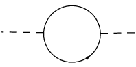
In perturbative quantum field theory stability, as well as unitarity, must be checked at the leading order. In general, this means at the tree level, but in the models of this paper one field, , has a dynamically generated propagator. At the leading order of the large expansion the -propagator is determined by a one-loop diagram (see fig. 2).
The spectral function must vanish for and be non-negative for . We can prove in complete generality that these requirements are automatically fulfilled. Call and the Minkowskian field and bubble diagram, respectively. The unitarity relation of fig. 1 tells us that the imaginary part of can be calculated using the cutting technique, it is convergent and non-negative. Therefore, at the leading order in we have , so the spectral function reads
and is necessarily non-negative. Moreover, writing the cutting diagram of explicitly, it is straightforward to check that vanishes for , both in our scalar and fermion models. The spectral representation (3.6), the other formulas from (3.1) to (3.9) and the cutting rules apply to the field with obvious adjustments.
Because of stability, the bosonic sectors of the classical action and of the generating functional of one-particle irreducible diagrams must be positive definite in the Euclidean framework. No general argument guarantees the positivity of the -sector of (counterexamples are easy to construct), therefore this aspect needs to be investigated in detail.
Regularity of the propagator
To verify the consistency of our theories, it is necessary, in addition, to check that the propagator be regular everywhere. Here denotes its weight. In particular, in the “ultraviolet” limits and , must behave as
| (3.12) |
respectively, to be consistent with the weighted power counting. For example, the propagator of (2.1),
is regular of weight 2, but a propagator of the form
is not regular, and could generate spurious ultraviolet sub-divergences in Feynman diagrams when tends to infinity at fixed, or viceversa (see ref. [9] for details). In some of our models (e.g. the one studied in section 8) regularity can be proved straightforwardly, in other models (e.g. the one studied in section 9) regularity is not fulfilled and the absence of spurious divergences has to be proved by direct analysis.
4 Causality
In this section we investigate causality at the classical and quantum levels. We work of course in the Minkowskian framework.
Classical theory
Consider the scalar field theory
coupled with an external source , where is a positive polynomial function. The field equations
| (4.1) |
are solved as
| (4.2) |
where is the retarded Green function. Decomposing as , we have
The retarded (advanced) Green function vanishes for negative (positive) time intervals, for an arbitrary function . Thus the solution (4.2) of the field equations (4.1) is determined by the sole knowledge of the source in the present and in the past, which ensures causality at the classical level.
Quantum theory
Bogoliubov’s definition of causality reads [17]
| (4.3) |
where denotes the -matrix and is a coupling constant, made into a function of spacetime. Formula (4.3) admits a more general single-diagram version [16], which reads
| (4.4) |
Here denotes a diagram in coordinate space with vertices in . No integral over the positions of the vertices is understood. The propagator connects two non-underlined points and , while connects a non-underlined point with an underlined point , connects with and connects with . Finally, every underlined vertex carries an extra minus sign.
The proof of (4.4) is done as follows. Call the vertex with the largest time component . By assumption, is not . Hence the sum (4.4) can be rearranged into the sum over pairs of diagrams differing only by being underlined or not. We want to show that the diagrams of each pair sum to zero. Indeed, they differ by an overall minus sign, because of the underlining, and have exactly the same propagators. To see this, let denote any vertex connected with . Since the identities
| (4.5) |
hold. Therefore, within each pair it does not matter whether is underlined or not, apart from the relative minus sign. We conclude that the sum (4.4) vanishes identically.
Finally, formula (4.3) is derived multiplying (4.4) by appropriate source functions, integrating over all points but and , and summing over all diagrams. The first term of (4.3) collects the diagrams where neither nor are underlined, while the second term of (4.3) collects the diagrams where is not underlined, but is.
5 Lifshitz type models
In this section we construct scalar models that have nontrivial interacting fixed points in the large expansion and study those fixed points. We classify the unitary, stable models and single out the four dimensional cases.
Consider the sigma model
| (5.1) |
in the Euclidean framework, where is a positive constant and is a field. Integrating over constrains the scalar field to live on a sphere of radius . The redundant parameter is introduced for convenience. The large expansion is defined as the expansion in , where is sent to infinity keeping finite.
The field does not have a kinetic term. In the large expansion the missing propagator is generated dynamically. Precisely, it is equal to minus the reciprocal of the scalar bubble of Fig. 2, whose form is (A.1) (in the case , , ). Every other diagram gives a subleading contribution.
The constant has a positive weight (for đ) and a positive dimensionality, therefore the UV fixed point is the same theory with :
| (5.2) |
Moreover, the term does not contribute to any non-trivial one-particle irreducible diagram, therefore the generating functionals and of (5.1) and (5.2) differ exactly by that term. For the same reason, once we prove the renormalizability of (5.2) we prove also the renormalizability of (5.1).
The theory (5.2) coincides with the Lifshitz fixed point of the -theory (2.8), which in the cases , đ has been studied in [6, 7]. Here we are interested in more general situations, so we allow đ to be greater than 4 and keep generic.
In the Minkowskian framework the lagrangian of the fixed point reads
| (5.3) |
which is Hermitian if is real.
Let us describe some basic properties of the theory (5.2), assuming for the moment that it is renormalizable as it stands. The conditions for renormalizability are worked out below. Since a renormalization constant in front of the vertex can be interpreted as the wave function renormalization constant (instead of the renormalization constant), the theory has no true coupling, although it is interacting. As a consequence, there is no running of couplings, so the model (5.2) is exactly invariant under the weighted scale transformation
| (5.4) |
also at the quantum level, once we include the rescaling of the RG scale .
Next, since the weight of must be positive, we have đ, which ensures also, from section 2, that Feynman diagrams do not contain IR divergences at non-exceptional external momenta. We have observed in section 4 that causality is always guaranteed. Nevertheless, unitarity, renormalizability and stability are not obvious and put other restrictions on the allowed values of đ.
Unitarity
In section 3 we have proved in complete generality that the spectral function of the field in the Minkowskian framework is non-negative and vanishes for . It remains to study the unitary bound (3.11). Since (5.2) is a homogeneous theory, is a homogeneous function. Since stands for , the weight of is equal to . On the other hand, the weight of is equal to minus the weight of the scalar bubble. We conclude that
for , so the unitarity bound gives đ.
Renormalizability
Now we study the counterterms. Since we use the dimensional-regularization technique, no power-like divergences are generated. The theory contains no weightful parameter (recall that is weightless), therefore every counterterm must be of weight đ. To have exact weighted scale invariance at the quantum level, (5.2) must be renormalizable as it stands, so no new vertex should be generated by renormalization. Indeed, a new vertex would be multiplied, in general, by a running coupling constant, so (5.2) would no longer be a fixed point of the RG flow. We need to classify all counterterms compatible with locality and weighted power counting. Consider first the counterterms of the form
| (5.5) |
We must exclude them for every even non-negative integer . The weight of (5.5) is , which by homogeneity must be equal to đ. Therefore we have
Now, this is negative for đ, and zero for đ. Thus đ must be excluded. Moreover, in the range đ we have to exclude every case where is even. This leaves only two situations: ) both and are odd; ) is even and is odd.
Next, consider
| (5.6) |
where the square bracket is used as a symbolic notation to denote any action of the derivatives on the fields. Equating the weight of (5.6) to đ we have
and since đ either or is necessarily negative for every . Therefore, the absence of (5.6) does not impose new restrictions on đ.
There exists only one term of weight đ containing both ’s and ’s, which is . Thus it remains to consider those counterterms that contain only fields. Any time a counterterm factorizes a it is proportional to the field equation, so it can be removed redefining the field . Consider the counterterms containing ’s and a certain number of derivatives
| (5.7) |
We do not need to consider derivatives since there would be at least two of them and then the counterterm would necessarily contain just two ’s and no , otherwise its weight would exceed đ. It is easy to prove that if is smaller than the counterterm (5.7) is always proportional to , up to total derivatives. Instead, if is at least , then there exists an arrangement, namely
that is not proportional to . Thus, writing , the counterterm (5.7) should be forbidden for every non-negative even integer . The weight condition gives
| (5.8) |
This formula implies that the counterterm (5.7) is automatically forbidden, or reabsorbable into the field equation, when
| (5.9) |
because then is negative. On the other hand, (5.8) also shows that if is odd is certainly even. In particular, the counterterm (5.7) with is forbidden or reabsorbable into the field equation if and only if (5.9) holds, namely
| (5.10) |
Luckily, (5.10) excludes also every counterterm (5.7) with , because it implies (5.9). Yet, it remains to exclude the counterterm with , which requires either
or one of the situations )-) mentioned before.
Summarizing, we have unitary renormalizable models in the following three situations:
| (5.11) | |||||
| (5.12) | |||||
| (5.13) |
We recall that ) means that both and are odd, while ) means that is even and is odd.
Stability
At the leading order in the expansion stability can be checked verifying that the -quadratic contribution to the generating functional is positive definite in the Euclidean framework. For đ the positivity of the two-point function is guaranteed. Indeed, the bubble (see (A.1)) is a convergent integral of a negative definite integrand (because of the factor ), so it is negative. The propagator is minus the reciprocal of the bubble, so it is positive. This argument does not apply for đ. Indeed, in that range the bubble diagram is formally divergent and stability has to be checked explicitly.
Regularity
For analogous reasons, the propagator is manifestly regular for đ. Indeed, since the bubble integral is convergent and its integrand is negative definite, setting or gives precisely the power-like behaviors (3.12) with đ. For đ regularity has to be checked explicitly case by case.
The models that satisfy (5.11) and (5.12) are guaranteed to be unitary, stable and regular. Let us list the four dimensional solutions. Clearly, must be , or . For , the unique solution is , with đ, , respectively, while for , can be an arbitrary even number greater than one, or equal to 3. The , đ four dimensional model is studied explicitly in section 8.
6 Four-fermion models
In this section we extend our analysis to the four fermion models. Start from the Euclidean four fermion lagrangian
| (6.1) |
for đ. This model is not renormalizable by weighted power counting, but, under certain conditions, it becomes renormalizable in the large expansion. Introduce an auxiliary field of weight 1 and rewrite the lagrangian as
| (6.2) |
In the large expansion the resummation of the bubble diagrams of Fig. 2 modifies the naive -propagator
into
where is the value of the bubble diagram (see (B.1) for an explicit expression in a concrete case). Because of the mass , super-renormalizable terms are generated by renormalization, proportional to integer powers of . For the moment we assume that no new strictly renormalizable vertex is turned on and later determine the conditions under which this effectively happens. Under these assumptions the complete renormalizable lagrangian reads
| (6.3) |
At is a homogeneous function of and and has the correct weight, equal to đ, to ensure the renormalizability of (6.3) by weighted power counting in the large expansion (see (8.2) for an example), if we assume that the propagator is regular (the conditions for its regularity are derived below). Observe that the beta function of (6.3) vanishes identically, since is a redundant parameter that can be reabsorbed in and . The renormalization constant of the vertex can be interpreted as the wave function renormalization constant.
Since vanishes at , we see that in the ultraviolet limit the four fermion theory (6.3) flows to the weighted scale invariant fixed point
| (6.4) |
whose Minkowskian lagrangian reads
| (6.5) |
with . Observe that (6.3) is an interesting example of asymptotically safe theory [18], its interacting UV fixed point being indeed (6.4)-(6.5).
Let us study the properties of the fixed point. First observe that (6.5) is invariant under parity:
but when is odd the theory is invariant also under reflection with respect to every space axis , precisely
| (6.6) |
Unitarity
The positivity of the spectral function is always guaranteed, for an argument analogous to the one of the previous section. The fermion bubble of Fig. 2 has weight equal to đ, so with đ. The unitarity bound (3.11) gives đ, therefore we are going to study the models with
| (6.7) |
Renormalizability
We now study the counterterms and impose that (6.4) be renormalizable as it stands, in particular that no new strictly renormalizable term be turned on. The conditions that we find ensure also the renormalizability of (6.3). First, the counterterm
| (6.8) |
must be forbidden for every non-negative even integer . Its weight must be equal to đ, so
Since đ we must have either ) , both odd, or ) even and odd.
We want to forbid also
| (6.9) |
for every non-negative integers , and every even . Indeed, when is odd the counterterm is already forbidden by the invariance under (6.6). In the other cases we have
The cases with đ are fine, because either or must be negative. The case đ ( even) is forbidden. Finally, when đ, even implies odd again.
It is easy to show that other terms such as
| (6.10) |
are automatically forbidden, for every even non-negative integers and and for every .
Next, observe that there is a unique parity-invariant vertex with both and fermion legs, that is . It remains to consider only the counterterms containing four or more fermions and no . The four-fermion terms are symbolically written as
| (6.11) |
Every non-negative integers and must be excluded. Equating the weight of (6.11) to đ we have
so these terms are automatically excluded for đ. The exclusion of counterterms of the form with is also guaranteed.
Summarizing, we have non-renormalizable models (that become renormalizable in the expansion) when
| (6.12) |
where, again, i) means that , are both odd, and ii) means that even and is odd. However, the case đ with even is excluded.
Let us list the four dimensional solutions to the conditions found so far. We can have or . When , the unique solution has , đ. When no solution is admitted. Finally, when every even is a solution. The simplest model of this class has , đ. It is studied explicitly in section 9, where we show that it is stable and regular, and calculate its subleading corrections.
Since the fermion bubble is always superficially divergent, in general stability and regularity have to be studied case by case. Nevertheless, there exists a noticeable class of odd-dimensional models that can be proved to be stable and regular with a simple argument.
Stability and regularity for odd
Write and set for simplicity. After a few straightforward steps the Euclidean fermion bubble can be written as
where , . We can replace with and with in the numerator, since the difference is a tadpole and vanishes identically using the dimensional-regularization technique. We get
| (6.13) |
Now the numerator is positive definite and the integral is convergent for
| (6.14) |
Therefore, when (6.14) holds the fermion bubble is negative-definite, which implies that the two-point function is positive definite and the theory is guaranteed to be stable. For the same reason, setting or in (6.13) gives the power-like behaviors (3.12) with đ, proving regularity.
The simplest example of solutions to (6.14) and (6.12) is the Lorentz invariant () four-fermion model in three spacetime dimensions [10]. For the solutions must have , since for (6.14) cannot be fulfilled. Then we find . These solutions generalize the four-fermion models of ref. [10] to arbitrary odd dimensions. Since is odd, the reflection symmetry (6.6) ensures that diagrams with an odd number of external -legs and no external -leg vanish identically. Therefore, in these models only the diagrams () and () of Fig. 3 contribute to the renormalization group flow up to the next-to-leading order.
7 Renormalization group
The fixed points of our Lorentz violating models are not conformal field theories, but they are exactly weighted scale invariant. They depend on the scale and have two correlation lengths (if the Lorentz group is split into two subfactors, more otherwise). The symmetry under weighted scale transformations is not sufficient to determine the two-point and three-point functions up to a finite number of constants. In this section we study the form of the two-point functions in the Lifshitz type models (5.2). The treatment is general and applies to the fermion models of section 6 with minor modifications.
We have wave-function renormalization constants for and and a renormalization constant for . They are just functions of . The bare quantities are
| (7.1) |
The Callan-Symanzik equation reads
| (7.2) |
where
Consider the two-point function . Because of the residual Lorentz invariance the correlation function depends only on . The RG equations tell us that
| (7.3) |
On the other hand, the invariance with respect to (5.4) gives
| (7.4) |
Finally, dimensional analysis gives
| (7.5) |
There is only one dimensionless combination of , , and that is RG invariant and invariant under (5.4), namely
therefore the solution contains an arbitrary function of it. The other dependencies can be fixed straightforwardly and the result is
Even simpler is the form of the two-point function in momentum space, which is
From the zeroth order propagator we have
8 Fixed points of scalar theories
In this section we give results about the four dimensional Lifshitz type fixed point (5.2) with , , , đ= up to the subleading order in the expansion. The model is perturbatively unitary, causal, stable and regular.
The scalar bubble (Fig. 2) is evaluated in appendix A. The -propagator has weight and it is equal to minus the reciprocal of (A.3), namely
| (8.1) |
where . The positivity of (8.1), which guarantees stability, is a direct consequence of the superficial renormalizability of the scalar bubble. The asymptotic behaviors in the limits and , namely
| (8.2) |
agree with the regularity conditions (3.12) in the ultraviolet limits and , respectively, and also prove smoothness in the infrared regions and , which guarantees the absence of spurious IR divergences. Finally, it is evident that the propagator (8.1) is manifestly regular everywhere else.
We now use the propagator (8.1) to compute the subleading corrections.
Subleading corrections

The corrections can be worked out computing the divergent parts of the diagrams , and drawn in Fig. 3. The dashed line is the -propagator (8.1). The continuous line denotes the scalar field. The orientation of the continuous line is immaterial in the scalar case, so the diagram is the same as and should not be counted. In the Lorentz-invariant three-dimensional models [11] the diagram is convergent, but in the four-dimensional model that we are considering now it is not. Nevertheless, the calculation of its divergent part can be luckily carried over to the very end, using the strategy illustrated in Appendix E. The results are
| (8.3) |
whence
| (8.4) |
The results (a), and agree with the ones found in ref. [7], while (b), (c) and are new.
9 Fixed points of fermion theories
With simple generalizations the techniques used in the previous section apply also to the four-dimensional fermionic model (6.4) with , , , đ. This model is perturbatively causal, unitary, stable and regular. Since the bubble is superficially divergent stability and regularity can be proved only by explicit computation, done in appendix B.
The -propagator has weight and can be read from (B.1):
| (9.1) |
Its positivity proves stability. The asymptotic behavior for , which is
| (9.2) |
agrees with the regularity condition (3.12) for and, at the same time, proves smoothness for . The asymptotic behavior for , instead,
| (9.3) |
does not agree with (3.12) and deserves more attention. When and is kept fixed (or grows more slowly than ) the behavior (9.3) could generate a spurious UV “sub”divergence in the integral over . Now we prove that it is not so. Consider a diagram with integrated momenta , loops, vertices, internal legs and external legs. Using , and , we get . Since, we obtain the bound . Each fermion propagator behaves like , so the degree of divergence of the subintegral over is
Spurious UV divergences () can occur only for , , which implies . The unique diagram with a potential problem is the one-loop fermion self energy (a). However, because of (9.3) in that case the potentially dangerous behavior reads
While the -integral is logarithmic divergent, it is multiplied by a -integral that vanishes identically in dimensional regularization. Thus the behavior (9.3) is not dangerous for .
Finally, when the behavior (9.3) guarantees that no spurious IR divergences affects the -integral at non-exceptional external hatted momenta. In every other region the propagator (9.1) is manifestly regular.
Subleading corrections
The contributing diagrams are , , and of Fig. 2. We find
| (9.4) |
whence
| (9.5) |
10 RG interpolation between pairs of fixed points
Following ref.s [19] and [20] in this section we construct RG flows interpolating between pairs of fixed points of the types studied in sections 8 and 9.
The interpolating theories have lagrangians
It is straightforward to prove the renormalizability of such models. The only caveat, with respect to the analysis of counterterms performed section 5 (for scalar fields) is that we must exclude also new counterterms proportional to , because they are no longer proportional to the field equations. Since đ= the weight of , is , so counterterms with four or more scalars are forbidden by locality.
In practice, the interpolating theories are made by pairs of models (5.2) or (6.4) sharing the same field . Here the parameter is suppressed (reabsorbed inside ) and the running couplings are and . The fixed points are the zeros of the and beta functions. There is an evident duality
| (10.1) |
The phase diagrams contain some remarkable fixed points. When the models tend to the fixed points (5.2) or (6.4) plus some free fields. When the models tend to the selfdual fixed points (5.2) or (6.4) with . Because of the duality (10.1), when the models tend to the fixed points (5.2) or (6.4) with , plus free fields. The phase diagrams might contain also some new fixed points.
The bubble diagrams of the interpolating models can be easily calculated using the results of the fixed points. We have the sum of two terms: the first contribution is due to circulating , fields and coincides with (A.3) or (B.1) (at ); the second contribution is due to circulating , fields and is equal to times (A.3) or (B.1), but with replaced by , where . In total we have
This formula proves stability and regularity in both interpolating models.
Only finitely many graphs contribute at each order of the large expansion, so the subleading corrections can be calculated exactly in , at every order in .
11 Conclusions
In this paper we have studied several properties of Lorentz violating quantum field theories of scalars and fermions and constructed fixed points of renormalization-group flows using a large expansion. Such fixed points have an exact weighted scale invariance and are the best generalizations of conformal field theories when the Lorentz symmetry is violated.
Unitarity, causality and stability can be generalized straightforwardly to Lorentz violating theories, because, strictly speaking, none of these notions demands Lorentz invariance. We have classified the models that are guaranteed to be unitary, causal and stable. In other models stability needs to be verified explicitly case by case. Solutions exist also in four and higher dimensions, while Lorentz invariant models of this type are known to exist only in lower dimensions. This makes our new models potentially interesting for applications to high-energy physics.
In some fixed points the calculations can be analytically carried over up to the subleading corrections. Using a simple trick it is also easy to construct running quantum field theories that interpolate between pairs of fixed points.
The models constructed here and in ref. [9] enlarge considerably the realm of renormalizable theories. They have a variety of potential physical applications and provide a large laboratory to test ideas about quantum field theory and renormalization.
Appendix A: Scalar bubble
Since some calculations in Lorentz violating theories have unusual aspects we collect details and results in these appendices.
We study the two-point function for the model (5.2) with , , , đ= at the leading order in . We first evaluate the bubble diagram of fig. 1 in the Euclidean framework. Later we compute the imaginary part in the Minkowskian framework using the cutting method. The graph reads
| (A.1) |
We integrate over using Feynman parameters and find
The integrand can be conveniently expanded in powers of . Using
| (A.2) |
and resumming the series, we arrive at
| (A.3) |
which agrees with the result of [7]. The contribution to the generating functional of one-particle irreducible diagrams is positive definite:
| (A.4) |
in agreement with stability.
We now rotate the correlation function to the Minkowskian framework and study the imaginary part of the scalar bubble. The lagrangian (5.2) is turned into (5.3). We find a cut on the real axis for . The imaginary part of the bubble multiplied by results
| (A.5) |
and can be checked also directly computing the cutting diagram of the self energy.
Appendix B: Fermion bubble
In this appendix we study the -two-point function of the model (6.4) with , , , đ at the leading order in . The strategy of the calculation is the same as in the previous section. The main difference with respect to the scalar case is that now the integral is formally divergent. The divergence is however power-like and so vanishes using the dimensional-regularization technique. First we integrate over the momentum using standard techniques. The result is
Next, it is convenient to expand the integrand in powers of and integrate the series term-by-term. The zeroth order term of the expansion, equal to , is killed by the dimensional integral over . The integral of every other term is convergent in and can be calculated again using (A.2). Resumming the series we obtain
| (B.1) |
Again, the contribution to the generating functional of one-particle irreducible diagrams is positive definite,
which proves stability.
The imaginary part of the Minkowskian bubble multiplied by is
Being positive definite, this result is a check that the theory is perturbatively unitary.
Appendix C: Scalar triangle
In this section we compute the scalar triangle with one vanishing external momentum. The triangle is necessary to compute the divergent part of the diagram . Denote the external momentum with and the loop momentum with . To avoid IR problems, we add a mass changing the scalar propagator as follows:
| (C.1) |
The diagram is ultraviolet convergent. First we integrate over using Feynman parameters, then over . The -integral gives
Next, the integral over is easily done using the residue theorem. The result can be expanded in powers of as
| (C.2) |
up to , where is defined in section 8. The masses in the denominators have been left, again, to avoid IR problems in the calculation of the two-loop diagram , which is performed in Appendix E.
Appendix D: Fermion triangle
Now we calculate the fermion triangle with one vanishing external momentum. The integral has no IR problem, so we do not need to introduce a mass. On the other hand, the diagram is formally ultraviolet divergent. The UV divergence is linear, so it vanishes in dimensional regularization. Equivalently, we can work in the physical dimension and subtract an appropriate local term. Again, the integration over the loop momentum is first done over using Feynman parameters, then over . Call the external momentum. The -integral gives
The integral over is easily done expanding the arctangent in powers of its argument, eliminating the first contribution to the sum (which subtracts the UV divergence) and using (A.2). Finally, resumming the series back, we find the result
Appendix E: Calculation of the diagrams (a), (b) and (c)
Here we describe the strategy to calculate the divergent parts of the diagrams (a), (b) and (c) of Fig. 3. We begin with the scalar self energy (a). By locality, invariance and weighted power counting, its divergent part is parametrized as
The constants and are calculated appropriately differentiating with respect to and and later setting . To avoid spurious IR divergences at it is useful to introduce a small mass, e.g. using modified propagators of the form (C.1). The coefficients and can be expressed as integrals
where is a certain homogeneous function of degree (giving a weight to ). Calling and changing variables from to we get an expression of the form
| (E.1) |
where is a function whose integral over is convergent. The factorized integral over gives instead the logarithmic divergence. Observe that in dimensional regularization the divergences are poles in [9], where and are the complex continuations of the dimensions and . In our calculation can be kept equal to zero to the very end, while the integral over needs to be continued in order to extract its UV divergence. We have
so in (E.1) the residue of the pole is the value of the -integral of .
The same strategy is used to calculate the other diagrams, both in the scalar and fermion models. Basically, a logarithmic divergent integral over is factored out. It multiplies a convergent integral over that can be evaluated exactly. In the case of fermions no IR divergence occurs at vanishing external momenta, so there is no need to introduce the mass .
Following these guidelights, the calculations proceed straightforwardly in all cases but one: the diagram (c) for scalar fields. As usual, its divergent part can be worked out setting its external momenta to zero and introducing an auxiliary mass. The triangle diagram with one vanishing external momentum, calculated in Appendix C, is sufficient for the evaluation. We know that the scalar triangle is IR divergent, as shown by formula (C.2). The first term of (C.2), however, vanishes when inserted in the rest of (c) and integrated. Indeed, this operation gives a result of the form , where is the value of some integral of weight . By weighted power counting, can only diverge linearly, and by locality its divergence can only have the form (not !). Therefore the divergent contribution due to the first term of (C.2) would depend on the sign of , which is absurd, since is introduced via the modified propagator (C.1). So, it is sufficient to keep the second term of (C.2). Once that term is inserted in the rest of (c) its manipulation is straightforward following the strategy described for diagram (a).
References
- [1] See for example, D.B. Kaplan, M.J. Savage and M.B.Wise, Nucleon-nucleon scattering from effective field theory, Nucl. Phys. B478 (1996) 629 and arXiv:nucl-th/9605002.
- [2] S. Weinberg, Phenomenological lagrangians, Physica A96 (1979) 327; For a review, see A.V. Manohar, Effective field theories, in Schladming 1996, Perturbative and nonperturbative aspects of quantum field theory, p. 311-362, arXiv:hep-ph/9606222.
- [3] See for example, O. Lauscher and M. Reuter, Ultraviolet fixed point and generalized flow equation of quantum gravity, Phys. Rev. D65 (2001) 025013 and arXiv:hep-th/0108040; H. Gies, J. Jaeckel and C. Wetterich, Towards a renormalizable Standard Model without a fundamental Higgs scalar, Phys. Rev. D69 (2004) 105008 and arXiv:hep-ph/0312034.
- [4] See for example P. Calabrese and A. Gambassi, Aging properties of critical systems, J. Phys. A38 (2005) R133 and arXiv:cond-mat/0410357.
- [5] T. Jacobson, S. Liberati and D. Mattingly, Lorentz violation at high energies: concepts, phenomena and astrophysical constraints, Annals Phys. 321 (2006) 150 and arXiv:astro-ph/0505267.
- [6] R.M. Hornreich, M. Luban and S. Shtrikman, Critical behavior at the onset of -space instability on the line, Phys. Rev. Lett. 35 (1975) 1678; See for example, M.M. Leite, Renormalization-group picture of the Lifshitz critical behavior, Phys. Rev. B 67 (2003) 104415.
- [7] M.A. Shpot, Yu.M. Pis’mak and H.W.Diehl, Large- expansion for -axial Lifshitz points, J. Phys. Condens. Matter 17 (2005) S1947 and arXiv:cond-mat/0412405.
- [8] D. Colladay and V.A. Kostelecký, Lorentz-violating extension of the Standard Model, Phys. Rev. D58 (1998) 116002 and arXiv:hep-ph/9809521; V.A. Kostelecký, Gravity, Lorentz violation, and the Standard Model, Phys. Rev. D 69 (2004) 105009 and arXiv:hep-th/0312310.
- [9] D. Anselmi and M. Halat, Renormalization of Lorentz violating theories, Phys. Rev. D 76 (2007) 125011 and arXiv:0707.2480 [hep-th].
- [10] G. Parisi, The theory of nonrenormalizable interactions. I – The large expansion, Nucl. Phys. B 100 (1975) 368.
- [11] I.Ya. Aref’eva, Phase transition in the three dimensional chiral field, Ann. Phys. 117 (1979) 393; I.Ya. Aref’eva and S.I. Azakov, Renormalization and phase transition in the quantum model (), Nucl. Phys. B 162 (1980) 298.
- [12] T. Banks and A. Zaks, On the phase structure of vector-like gauge theories with massless fermions, Nucl. Phys. B 196 (1982) 189.
- [13] See for example, N. Seiberg, Electric-magnetic duality in supersymmetric non-Abelian gauge theories, Nucl. Phys. B 435 (1995) 129 and arXiv:hep-th/9411149; D. Anselmi, D.Z. Freedman, M.T. Grisaru and A.A. Johansen, Nonperturbative formulas for central functions of supersymmetric theories, Nucl. Phys. B 526 (1998) 543 and hep-th/9708042.
- [14] D. Anselmi, Renormalizable Lorentz violating gauge theories, in preparation.
- [15] V.A. Kostelecký, C.D. Lane and A.G.M. Pickering, One-loop renormalization of Lorentz-violating electrodynamics, Phys. Rev. D 65 (2002) 056006 and arXiv:hep-th/0111123; D. Colladay and P. McDonald, One-Loop renormalization of pure Yang-Mills with Lorentz violation, Phys. Rev. D 75 (2007) 105002 and arXiv:hep-ph/0609084.
- [16] G. ’t Hooft and M. Veltman, Diagrammar, report CERN-73-09, available at http://cdsweb.cern.ch/record/186259 .
- [17] N.N. Bogoliubov and D.V. Shirkov, Introduction to the theory of quantized fields, Interscience Publishers, New York, 1959.
- [18] S. Weinberg, Ultraviolet divergences in quantum theories of gravitation, in An Einstein centenary survey, Edited by S. Hawking and W. Israel, Cambridge University Press, Cambridge 1979.
- [19] D. Anselmi, Large- expansion, conformal field theory and renormalization-group flows in three dimensions, JHEP 06 (2000) 042 and hep-th/0005261.
- [20] D. Anselmi, “Integrability” of RG flows and duality in three dimensions in the 1/ expansion, Nucl. Phys. B 658 (2003) 440 and hep-th/0210123.