$G$ -Parking Functions, Acyclic Orientations and Spanning Trees

Brian Benson Address: B. Benson, Department of Mathematics, University of Illinois, Urbana-Champaign, Illinois Email address: benson9@illinois.edu , Deeparnab Chakrabarty Address: D. Chakrabarty, Department of Combinatorics & Optimization, University of Waterloo, Waterloo, Ontario N2L 3G, Canada Email address: deepc@math.uwaterloo.ca and Prasad Tetali Address: P. Tetali, School of Mathematics and School of Computer Science, Georgia Institute of Technology, Atlanta, GA 30332-0160. Email address: tetali@math.gatech.edu

Abstract.

Given an undirected graph $G=(V,E)$ , and a designated vertex $q\in V$ , the notion of a $G$ -parking function (with respect to $q$ ) was independently developed and studied by various authors, and has recently gained renewed attention. This notion generalizes the classical notion of a parking function associated with the complete graph. In this work, we study properties of maximum $G$ -parking functions and provide a new bijection between them and the set of spanning trees of $G$ with no broken circuit. As a case study, we specialize some of our results to the graph corresponding to the discrete $n$ -cube $Q_{n}$ . We present the article in an expository self-contained form, since we found the combinatorial aspects of $G$ -parking functions somewhat scattered in the literature, typically treated in conjunction with sandpile models and closely related chip-firing games.

1. Introduction

The classical parking functions provide a bijective correspondence between the spanning trees of the complete graph $K_{n}$ and certain integer-valued functions on the vertices of $K_{n}$ . A notion of parking functions corresponding to the spanning trees of an arbitrary graph $G$ is more recent and has been independently developed in physics and combinatorics. It was introduced by Bak, Tang and Wisenfeld [1] as a self-organized sandpile model on grids, and was generalized to arbitrary graphs by D. Dhar [17]. See Definition 2.1 below for the precise definition of a $G$ -parking function, associated with a connected graph $G$ .

This notion is already rather powerful; besides generalizing the classical parking function from $K_{n}$ to an arbitrary graph, it has been investigated in the context of chip-firing games [8, 29, 30] and the Tutte polynomial [9, 14] in discrete mathematics, and also investigated in algebra and related fields [2, 16, 31]. However, some of the combinatorial aspects of this topic appear somewhat scattered in the literature.

Several fundamental results concerning the recurrent configurations of chip-firing can be derived without the chip-firing context and terminology. For this reason, we shy away from introducing and discussing the chip-firing terminology. Instead, in this article we describe various interpretations of the $G$ -parking functions in the most elementary combinatorial ways. Using a natural partial order $\prec$ on the set ${\mathcal{P}}(G,q)$ of parking functions, we consider the maximal elements in this poset $\bigl({\mathcal{P}}(G,q),\prec\bigr)$ . Much of our focus in this paper is on understanding the properties of such maximal parking functions. The first result we describe (see Theorem 4.1) provides a new bijection between the maximal parking functions in the poset and the set $\mathcal{A}(G;q)$ of acyclic orientations of $G$ with a unique source at $q$ . En route, we describe what we call an Extended Dhar algorithm (since it is an extension of an algorithm due to Dhar [17] to recognize $G$ -parking functions) in providing an acyclic orientation corresponding to a maximal parking function. We review various combinatorial consequences and algebraic connections of this correspondence. For example, using known results (namely those of Greene and Zaslavsky [24] and more recent work of Gebhard and Sagan [21]), we further identify a 1-1 correspondence between the set of maximal parking functions and the set of spanning trees with no “broken circuits,” or equivalently, the set of “safe” spanning trees ; see Section 4 for the definitions of these terms. In this paper, we provide a much simpler bijection (compared to [21]) between the set of safe trees and the set of acyclic orientations with a unique sink (or equivalently, a unique source). Furthermore we generalize this bijection to one between all spanning trees and all $G$ -parking functions which preserves the bijection between safe trees and maximal $G$ -parking functions. We must remark here that other bijective proofs between the set of $G$ -parking functions and the set of spanning trees of $G$ (for arbitrary connected $G$ ) have been given by Chebikin and Pylyavskyy [13]. However, to our knowledge, the simpler bijection we report here, in Theorem 4.2 below, and its generalization given in Theorem 4.6, are indeed new.

As an additional contribution, we describe a simple way to generate maximal parking functions in the Cartesian product graph $G_{1}\Box G_{2}$ , using maximal functions in the (factor) graphs $G_{1}$ and $G_{2}$ . We then specialize our study to understanding the parking functions in the discrete $n$ -cube $Q_{n}$ on $2^{n}$ vertices. By describing certain special constructions of maximal parking functions $f$ on $Q_{n}$ , we obtain a natural description of a set, ${\rm dom}(f)$ , of parking functions – those dominated, in the partial order given by $\prec$ , by a special maximal parking function $f$ . Interestingly enough we shall deduce (see Theorem 5.2) that

(1.1)

|{\rm dom}(f)|=\prod_{k=2}^{n}k^{{n\choose k}}\,,

while it is a well-known fact that

(1.2)

|{\mathcal{P}}(Q_{n},q)|=\prod_{k=2}^{n}(2k)^{{n\choose k}}=2^{2^{n}-n-1}\,\,\prod_{k=2}^{n}k^{{n\choose k}}\,.

Recall that (1.2) corresponds to the total number of spanning trees of $Q_{n}$ (see equation (5.85) in [32]), using the matrix-tree theorem and the explicit knowledge of the corresponding eigenvalues, to help evaluate the determinantal formula. In light of the fact that finding a bijective proof accounting for the number of spanning trees of $Q_{n}$ has been open for several years, we hope this is a nontrivial step towards such a proof.

The paper is organized as follows. In Section 2, we review some preliminaries, including Dhar’s burn criterion, which determines whether a given function is a parking function. In Section 3, we show the bijection between maximum parking functions and acyclic orientations with a unique source. In Section 4.1, we describe our new and simpler bijection between the set of acyclic orientations with a unique sink and the set of safe trees. In Section 5.1, we describe a construction of maximum parking functions on Cartesian products of graphs. In Section 5.2, we focus our study on the $n$ -cube $Q_{n}$ , and provide some explicit constructions of maximum parking functions and related bounds. In Section 6, for expository purposes we review a bijection between diffuse states (introduced in the context of chip-firing) and acyclic orientations of a graph. We conclude with some remarks on research in future directions and a few open problems in Section 7.

2. $G$ -Parking Functions and Dhar’s Burn Criteria

In this section we recall the definition of a $G$ -parking function and review Dhar’s (burning) algorithm that can be used to determine whether an integer-valued function on the vertices of $G$ is a $G$ -parking function.

Definition 2.1.

For a connected graph $G$ , a $G$ -parking function relative to vertex $q\in G$ is a function $f:V(G){\rightarrow}{\mathbb{Z}}_{\geq-1}$ such that $f(q)=-1$ and for every non-empty $A\subseteq V(G)\backslash\{q\}$ , there exists $v\in A$ such that $0\leq f(v)<d_{\overline{A}}(v)$ , where $d_{\overline{A}}(v)$ is the number of edges $e=vw$ with $w\notin A$ .

Remark 2.1.

Herein, we have modified the standard definition of a $G$ -parking function somewhat. The function $f$ is now defined on all of $V(G)$ instead of restricted to simply $V(G)\backslash\{q\}$ in order to improve the compatibility between $G$ -parking functions and Cartesian product graphs such as $Q_{n}$ ; due to this change, for $f$ to be a $G$ -parking function, $f(q)=-1$ necessarily.

Proposition 2.1.

If for a function $f:V(G)\backslash\{q\}{\rightarrow}{\mathbb{Z}}_{\geq 0}$ , for every non-empty connected subgraph $A\subseteq G\backslash\{q\}$ , there exists $v\in V(A)$ such that $f(v)<d_{\overline{A}}(v)$ , then $f$ is a $G$ -parking function.

Proof. Assume that, for all connected $A\subseteq G\backslash\{q\}$ , that there exists $v\in V(A)$ such that $f(v)<d_{\overline{A}}(v)$ . Proceeding by contradiction, suppose that there is some disconnected $B\subseteq G\backslash\{q\}$ such that $f(v)\geq d_{\overline{B}}(v)$ for every $v\in V(B)$ . Consider then any connected component $C$ of $B$ . Since $C$ is connected we have, by the hypothesis of the proposition, that $f(v)<d_{\overline{C}}(v)$ , for some vertex $v$ in $C$ . Thus $d_{\overline{B}}(v)<d_{\overline{C}}(v)$ , implying that there is a vertex $u$ in $\overline{C}\backslash\overline{B}$ such that $v$ and $u$ are connected by an edge in $G$ ; otherwise, either $f(v)\geq d_{\overline{C}}(v)$ or $f(v)<d_{\overline{B}}(v)$ . This contradicts the choice of $C$ .

Throughout we assume that the reference vertex $q$ is fixed, and we always consider parking functions with respect to this fixed vertex $q$ , without necessarily bringing explicit reference to it.

A natural question to ask is whether a given integer-valued function on the vertices of $G$ can easily be tested for being a $G$ -parking function. In the context of the so-called sandpile models, Dhar [17] provided an algorithm, which can be interpreted as an efficient algorithm to test if a given function is a $G$ -parking function. This was observed in [13], wherein the algorithm was reformulated as follows. Let $f:V\setminus\{q\}\to{\mathbb{Z}}^{+}$ . We assume that $f(q)=-1$ .

Step 1. Mark any unmarked vertex $v$ which has more marked neighbors than $f(v)$ .

Step 2. Repeat Step 1 until no more vertices can be marked.

Step 3. Declare $f$ to be a $G$ -parking function if and only if all the vertices have been marked.

We omit the proof of correctness of the algorithm (as an exercise), which follows in a fairly straightforward way from the definition of a parking function.

On the set ${\mathcal{P}}(G,q)$ of parking functions on $G$ with respect to $q$ , there is a natural partial order we may define:

Definition 2.2.

Given two parking functions $f,g\in{\mathcal{P}}(G,q)$ , we say $g\prec f$ , if $g(v)\leq f(v)$ , for all $v\in V$ . The maximal elements in this partial order will be referred to as maximal parking functions. Finally, a parking function with the largest sum is called a maximum parking function.

For $f\in{\mathcal{P}}(G,q)$ , let $\|f\|:=\sum_{v}f(v)$ , and ${\rm dom}(f)=\{g\in{\mathcal{P}}(G,q):g\prec f\}$ . Furthermore, for $f,g\in{\mathcal{P}}(G,q)$ , let $f\wedge g$ be the function on vertices, defined as $f\wedge g(v):=\min\{f(v),g(v)\}$ , for each $v\in V(G)$ .

While the following propositions are perhaps folk-lore, the first part of Proposition 2.2 and Proposition 2.3 appear as Lemmas 7 and 5 in [9].

Proposition 2.2.

(a) Let $f\in{\mathcal{P}}(G,q)$ , and suppose $g:V(G){\rightarrow}{\mathbb{Z}}_{\geq-1}$ such that $g(q)=-1$ and $0\leq g(v)\leq f(v)$ , for $v\in G$ with $v\neq q$ . Then $g\in{\mathcal{P}}(G,q)$ .

(b) If $f,g\in{\mathcal{P}}(G,q)$ , then $f\wedge g\in{\mathcal{P}}(G,q)$ and ${\rm dom}(f\wedge g)={\rm dom}(f)\cap{\rm dom}(g)$ .

Proof. While Part (a) is clear from the definition of a $G$ -parking function, it can also be seen using Dhar’s algorithm.

Note that $f\wedge g(q)=-1$ and so $f\wedge g\in{\mathcal{P}}(G,q)$ , by Part (a). Now $f\wedge g\prec f$ and $f\wedge g\prec g$ , so $h\in{\rm dom}(f\wedge g)$ implies that $h\in{\rm dom}(f)\cap{\rm dom}(g)$ . Finally consider, $h\in{\rm dom}(f)\cap{\rm dom}(g)$ . Then at each vertex $v\in V(G)$ , $h(v)\leq f(v)$ and $h(v)\leq g(v)$ , so $h(v)\leq\min\{f(v),g(v)\}=f\wedge g(v)$ , proving that $h\in{\rm dom}(f\wedge g)$ .

Proposition 2.3.

For every connected graph $G=(V,E)$ , every $f\in{\mathcal{P}}(G,q)$ , we have $\|f\|\leq|E|-|V|$ . More over, the equality is always achieved.

Proof. We may prove this by induction on the number $n\geq 1$ of vertices $G$ . The base case consisting of $V=\{q\}$ and no edges is trivially true. For the induction case, let $n\geq 2$ . Given $f\in{\mathcal{P}}(G,q)$ , let $v_{n}$ be the last vertex to be marked by the Dhar algorithm. Then consider $H:=G\setminus\{v_{n}\}$ , the graph obtained by removing $v_{n}$ and its incident edges. $H$ is connected, since Dhar successfully marks all vertices before $v_{n}$ , and more over, the function $f_{H}$ denoting, $f$ restricted to $H$ , is an $H$ -parking function with respect to $q\in H$ . Thus we may apply the induction hypothesis to $H$ and $f_{H}$ and complete the proof:

\|f\|=f(v_{n})+\|f_{H}\|\leq\sum_{v\neq v_{n}}f(v)\leq d(v_{n})-1+\bigl(|E|-d(v_{n})\bigr)-(|V|-1)\leq|E|-|V|\,,

where we also used the fact that $f(v)\leq d(v)-1$ , for every $v$ and parking function $f$ .

The proof also suggests that by assigning the maximum possible value, at each step in Dhar’s marking algorithm, one easily obtains a (maximum) parking function which achieves the upper bound.

Note that the quantity ${\bf g}(G):=|E|-|V|+1$ is sometimes referred to as the cyclomatic number or the Betty number of the graph and due to our convention of assigning $f(q):=-1$ , we have ${\bf g}(G)-1$ , as the bound in the above proposition.

Proposition 2.2 also gives us a simple (albeit not necessarily efficient), inclusion-exclusion method to relate the set of maximum parking functions with the set of all parking functions. But this has to wait until the next section, where we observe another basic fact concerning the maximum parking functions.

3. Maximal $G$ -Parking Functions and Acyclic Orientations with a Unique Source

Given a graph $G$ , the notion of an acyclic orientation of the edges of $G$ is classical, with an extensive literature. The notion of an acyclic orientation with a unique source at a fixed vertex is less well-studied. Let ${\rm AO}(G)$ denote the set of acyclic orientations of the graph $G$ and let $\mathcal{A}(G,q)$ be the set of acyclic orientations of $G$ with a unique source at vertex $q$ . Finally, let ${\rm MP}(G,q)$ denote the set of maximum $G$ -parking functions.

Theorem 3.1.

There exists a bijection between $\mathcal{A}(G,q)$ and the set ${\rm MP}(G,q)$ of maximum $G$ -parking functions.

Proof. Given an acyclic orientation ${\mathcal{O}}\in\mathcal{A}(G,q)$ with a unique source at $q$ , define the function $f=f({\mathcal{O}})$ on the vertices of $G$ : let $f(v)$ be the indegree (in ${\mathcal{O}}$ ) of $v$ minus 1. We will show that this correspondence provides the necessary bijection.

In any orientation, the sum of the indegrees equals the number of edges. Hence $\sum_{v}f(v)=|E|-|V|$ . By using Dhar’s algorithm, we may show that $f$ is in fact a parking function: starting with $q$ , we may repeatedly mark and remove the current set of source(s) in the acyclic orientation of the remaining graph; since a vertex $v$ with value $f(v)$ becomes a source only when all its $f(v)+1$ in-neighbors have been marked and removed, the Dhar criterion is satisfied. Also observe that the procedure stops only after marking all the vertices, since every acyclic orientation has at least one source. Thus $f({\mathcal{O}})\in{\rm MP}(G,q)$ .

To see that $f({\mathcal{O}}_{1})\neq f({\mathcal{O}}_{2})$ , whenever ${\mathcal{O}}_{1}\neq{\mathcal{O}}_{2}$ , simply recall that an acyclic orientation is uniquely determined by its outdegree sequence: starting with the sinks, orient all edges into the sinks, remove the sinks, and repeat the process by subtracting one from the outdegrees of the neighbors of the sinks.

The proof will be complete once we establish the onto property, that every maximum parking function can be obtained this way. Given a maximum parking function $f\in{\rm MP}(G,q)$ , we will construct an orientation ${\mathcal{O}}(f)$ using the following modification of Dhar’s algorithm, and will show that ${\mathcal{O}}(f)\in\mathcal{A}(G;q)$ , thus essentially providing an inverse map to the above construction.

The Extended Dhar Algorithm.

Input: A maximal parking function $f\in{\rm MP}(G,q)$

Output: An acyclic orientation ${\mathcal{O}}(f)$ with a unique source at $q$ .

Step 1. Start with $v=q$ . Orient all edges out of $q$ .

Step 2. If there exists a vertex $v$ which accrued indegree( $v$ ) equal to $f(v)+1$ , mark $v$ and orient the remaining edges incident at $v$ outward from $v$ .

Step 3. Repeat Step 2, until all vertices are marked and all edges are oriented.

The correctness of the original Dhar algorithm guarantees that all vertices will eventually be marked – indeed, the indegree( $v$ ) equals the number of neighbors marked before $v$ ; thus all edges will be oriented, meaning that ${\mathcal{O}}(f)$ is an orientation of the edges of $G$ . Observe that the indegree of a vertex $v$ equals $f(v)+1$ . Since $q$ is unique with $f(q):=-1$ , it must be that $q$ is the unique source. It is also easy to see that ${\mathcal{O}}(f)$ is acyclic – if there were to be a cycle, considering the first vertex in the cycle which was marked, we obtain a contradiction to the way the edges were oriented (in Step 2 above) from a marked vertex.

Remark 3.1.

Upon completion of this work, we discovered (thanks to Matt Baker), that Theorem 3.1 can also be derived using chip-firing games: As described in [23], the notion of a so-called diffuse state (introduced by [25] and see Definition 6.1 below) helps relate chip-firing configurations to acyclic orientations. Also thanks to an anonymous referee of an earlier version of this work [6], we learned that Theorem 3.1 is Lemma 10 (under the name of allowable orientations) of Biggs [9], where it is mentioned that this in fact goes back to an even earlier result of Greene and Zaslavsky [24].

It is now easy to observe the following fact (which appears as Lemma 8 in [8]).

Corollary 3.2.

Every maximal parking function is a maximum parking function.

Proof.

This follows from the proof of correctness of the Extended Dhar algorithm described above – if $f$ were maximal, but not maximum, then there must be a vertex in Dhar’s marking whose indegree is at least $f(v)+2$ . But then we can increase $f(v)$ by one, and obtain a valid parking function, contradicting the maximality of $f$ .

We now return to prove the simple result that was promised at the end of the previous section.

Corollary 3.3.

Let $G$ be a finite graph with $k$ maximum $G$ -parking functions. Then there exist $G$ -parking functions $f_{1},\ldots,f_{n}$ such that the number of $G$ -parking functions is

\sum_{i=1}^{n}\pm|{\rm dom}(f_{i})|\,,

where $n=2^{k}-1$ and the sign $+$ or $-$ is uniquely determined by Proposition 2.2.

Proof. Let $g_{1},g_{2},\ldots,g_{k}\in{\mathcal{P}}(G,q)$ be all the maximum $G$ -parking functions. Trivially, every non-maximal parking function is dominated by some maximal parking function, and Corollary 3.2 lets us observe that,

{\mathcal{P}}(G,q)=\cup_{i=1}^{k}{\rm dom}(g_{i})\,.

Now we may simply use the inclusion-exclusion formula to count the size of the union of the above $k$ sets:

$\displaystyle\|{\mathcal{P}}(G,q)\|$	$\displaystyle=$	$\displaystyle\|\cup_{i=1}^{k}{\rm dom}(g_{i})\|$
	$\displaystyle=$	$\displaystyle\sum_{i}\|{\rm dom}(g_{i})\|-\sum_{1\leq i<j\leq k}\|{\rm dom}(g_{i})\cap{\rm dom}(g_{j})\|+\cdots$
		$\displaystyle+(-1)^{k}\|{\rm dom}(g_{1})\cap{\rm dom}(g_{2})\cap\cdots\cap{\rm dom}(g_{k})\|$
	$\displaystyle=$	$\displaystyle\sum_{i}\|{\rm dom}(g_{i})\|-\sum_{1\leq i<j\leq k}\|{\rm dom}(g_{i}\wedge g_{j})\|+\cdots+(-1)^{k}\|{\rm dom}(g_{1}\wedge g_{2}\wedge\cdots\wedge g_{k})\|\,,$

which, upon using Proposition 2.2, completes the proof.

It would indeed be interesting to see if the above corollary can be used in making progress towards obtaining a bijective proof for the number of spanning trees of $Q_{n}$ , the $n$ -dimensional hypercube. In Section 5.2, we take a modest step towards it.

Theorem 3.4.

Let $G$ be a simple, connected graph. Then, for a fixed choice of $q$ , $G$ has a unique maximum $G$ -parking function if and only if $G$ is a tree.

Proof. If $G$ is a tree, then there is only one parking function with respect to any $q$ since $G$ has no cycles and, thus, each vertex can have at most one marked neighbor in the Dhar algorithm. (Note that this is in fact tautological if one uses the bijection between the parking functions and the spanning trees of $G$ .) Hence there is only one maximum $G$ -parking function.

The other direction is less obvious. However, observe that in light of the bijection established in Theorem 3.1, it suffices to show the following. Whenever $G$ is connected and contains a cycle, then there are at least two acyclic orientations for $G$ , with $q$ as the unique source. This is easy to establish (for example, by considering the standard directed acyclic graph (DAG) representation of the graph), and we leave the proof as a simple exercise.

See Remark 4.1 below for another short (but indirect) proof of the above theorem.

Corollary 3.5.

A simple, connected graph $G$ has a unique maximum parking function $f$ if and only if the range of $f$ is a subset of $\{-1,0\}$ .

Proof. This follows from the observation that any tree has a unique parking function and, for any vertex $v\neq q$ , $f(v)=0$ .

Corollary 3.6.

For every $G$ , $|{\mathcal{P}}(G,q)|=1$ if and only if $|{\rm MP(G,q)}|=1$ .

4. Bijections of Maximal $G$ -parking Functions

We now augment our Theorem 3.1 above to show a bijection between maximal $G$ -parking functions and spanning trees with no broken circuits. Before stating the theorem, we need to recall several definitions from the literature.

The Tutte (or Tutte-Whitney) polynomial of a graph $G=(V,E)$ is the two-variable polynomial defined as

(4.1)

{\mathcal{T}}_{G}(x,y)=\sum_{A\subseteq E}(x-1)^{\kappa(A)-\kappa(E)}\,(y-1)^{|A|-n+\kappa(A)}\,,

where $n=|V|$ and $\kappa(A)$ denotes the number of connected components of the graph on $V$ using edgeset $A$ . For $\lambda\in{\mathbb{Z}}^{+}$ , the chromatic polynomial $\chi_{G}(\lambda)$ of a graph $G$ is defined as the number of proper vertex colorings of $G$ using $\lambda$ colors. For a general variable $\lambda$ , the following relation between the chromatic polynomial and the Tutte polynomial is well-known (see e.g. [4, 5, 33, 34, 35]):

(4.2)

\chi_{G}(\lambda))=(-1)^{n-\kappa(G)}\,\lambda^{\kappa(G)}\,{\mathcal{T}}_{G}(1-\lambda,0)\,,

where $n=|V|$ is the number of vertices and $\kappa(G)$ is the number of connected components of $G$ .

Definition 4.1.

Given a graph $G=(V,E)$ and an ordering of all the edges of $G$ , a broken circuit $B\subseteq E$ is any cycle (of edges) of $G$ minus the largest (according to the ordering) edge in the cycle.

Note that since every cycle contains (or gives rise to) a broken circuit, a collection of edges not containing a broken circuit must necessarily be acyclic. Inspired by the terminology of Kenyon and Winkler [27], we call a spanning tree $T$ safe, if it contains no broken circuits. That is, for all edges $e$ not in the tree, there is an edge in the unique cycle formed when $e$ is added to the tree, which is larger than $e$ . The notion of a broken circuit is more general, and in fact explains the classical terminology: in the context of a matroid, an independent set of elements of the matroid obtained from a circuit, by removing the largest element (once again, according to some a priori global ordering of all the elements) of the circuit.

Theorem 4.1.

For every undirected, connected graph $G$ , the following quantities are all the same.

•

(a) The number of maximum $G$ -parking functions with respect to $q$ .
•

(b) The number of acyclic orientations with a unique source at $q$ .
•

(c) The number of spanning trees with no broken circuits, or equivalently, with zero external activity.
•

(d) The coefficient (up to sign) of the $\lambda$ -term in the chromatic polynomial $\chi_{G}(\lambda)$ .
•

(e) The value (up to sign) ${\mathcal{T}}_{G}(1,0)$ of the Tutte polynomial ${\mathcal{T}}_{G}(x,y)$ , evaluated at $x=1$ and $y=0$ .

Proof.

Theorem 3.1 shows the equivalence of (a) and (b). The equivalence between (c) and (d) is classical and is part of Whitney’s Broken Circuit theorem [35]: that the chromatic polynomial on $n$ vertices is given by

\chi_{G}(\lambda)=\sum_{r=0}^{n-1}(-1)^{j}m_{r}\lambda^{n-r},

where $m_{j}$ is the number of $r$ -subsets of edges of $G$ which contain no broken circuit. The term $m_{n-1}$ corresponds to (the absolute value of) the coefficient of $\lambda$ ; note that the $n-1$ -subsets under consideration being necessarily acyclic, correspond to spanning trees which do not contain a broken circuit.

The equivalence between (b) and (d) is due to Greene and Zaslavsky [24]. A (direct) bijective proof of the equivalence between (b) and (c) is given by Gebhard and Sagan [21], using a modification of an algorithm of Blass and Sagan [12]. In Section 4.1 we provide a much shorter proof of the equivalence between (b) and (c).

The equivalence between (d) and (e) follows from (4.2), and using $\kappa(G)=1$ , for a connected $G$ . The equivalence between (a) and (e) follows from results of [17] and [29], which confirmed a conjecture of Biggs [8] in the context of chip-firing. An inductive proof (using edge deletions and contractions) without involving chip-firing is due to Plautz and Calderer [30]. As described in [30], the work of Dhar and Lopez provides the following result:

{\mathcal{T}}_{G}(1,y)=\sum_{f\in{\mathcal{P}}(G,q)}y^{w(f)}\,,

where $w(f)=|E(G)|-|V(G)|+\|f\|$ , hence the equivalence of (a) and (e). The results in [29] and [14] also establish the equivalence between (c) and (e), with the minor modification that broken circuits are equivalently described using external acitivities - each broken circuit contributes an external activity of one to a spanning tree.

In addition to the above, Cori and Le Borgne [14] describe certain decreasing traversals of vertices and edges and a notion of strong edges to provide a bijection between recurrent chip-firing configurations (with a fixed “level”) and spanning trees with a fixed “external activity”. While the level corresponds to the sum of the values of a parking function (up to an additive shift), the external activity reflects the number of broken circuits, and we refer the interested reader to their paper for additional information.

Remark 4.1.

Observe that the nontrivial part of Theorem 3.4 follows easily using the equivalence between (a) and (c). Indeed, let $G$ be a connected graph which contains a cycle of length 3 or more. Then given a spanning tree which contains no broken circuit, we include an edge not in the tree to form a cycle $C$ . Since $C$ is of length 3 or more, there must be an edge, which is not the largest edge in the cycle, that can be removed, giving another spanning tree with no broken circuits. Hence a (connected) graph containing a cycle has more than one parking function.

4.1. Bijection between Acyclic Orientations with Unique Sink and Safe Trees

In this section we give a shorter proof, of equivalence of (b) and (c) of Theorem 4.1, than the ones reported in Gebhard and Sagan [21] and Gioan and Las Vergnas [22]. Note that the bijection in [21] is not activity-preserving while the one in [22] is; also see [28].

For ease of presentation, we will consider orientations with a unique sink rather than a unique source – clearly this is equivalent.

Let $\sigma$ be any total ordering of the edges of $G$ . Given two edges $e$ and $f$ , we say $e$ is larger than $f$ if $\sigma(e)>\sigma(f)$ . Similarly we say $e$ is smaller than $f$ , if the inequality is otherwise. Recall, a spanning tree $T$ of $G$ is called safe with respect to $\sigma$ if for any edge $e\notin T$ , there exists at least one edge $f$ in the unique cycle in $T+e$ such that $f$ is larger than $e$ . Let $\mathcal{T}(G,\sigma)$ be the set of safe trees with respect to $\sigma$ , and let $\mathcal{A}(G,q)$ be the set of acyclic orientations of $G$ with $q$ being the unique sink.

Theorem 4.2.

For any total order $\sigma$ , there exists a bijection $\mu_{\sigma}:\mathcal{T}(G,\sigma)\to\mathcal{A}(G,q)$ .

Henceforth, we fix $\sigma$ and do not write it as a subscript. Before we proceed, we make a few more definitions and observations. An arborescence with root $q$ is a directed spanning tree with all vertices except the root having out-degree exactly $1$ , and the root having out-degree $0$ . Any spanning tree corresponds to a unique arborescence with root $q$ and henceforth we will use the terms interchangeably. Given a vertex $i$ , we let $P_{i}$ denote the unique directed path from $i$ to $q$ . Given vertex $i$ and $j$ , we let $meet(i,j)$ be the first vertex in the intersection of $P_{i}$ and $P_{j}$ . That is, the path from $i$ to $meet(i,j)$ and the path from $j$ to $meet(i,j)$ are disjoint except at $meet(i,j)$ . If $j$ lies on $P_{i}$ , we let $j$ be $meet(i,j)$ . Observe that for three vertices $i,j,k$ , either (a) $meet(i,k)=meet(j,k)$ , or (b) $meet(i,k)$ lies on $P_{i}$ and $meet(j,k)=meet(i,j)$ , or (c) $meet(j,k)$ lies on $P_{j}$ and $meet(i,k)=meet(i,j)$ . Given two vertices $i$ and $j$ , we will denote the largest edge in the path from $i$ to $meet(i,j)$ as $e_{ij}$ and the largest edge from $j$ to $meet(i,j)$ as $e_{ji}$ . If $j=meet(i,j)$ , we let $e_{ji}$ be the null edge.

We (abuse notation and) say $i>_{\sigma}j$ if $e_{ij}$ is larger than $e_{ji}$ . We will also define $e_{ii}$ to be a null edge. Note that if $i>_{\sigma}j$ and $j>_{\sigma}k$ , then going over the three possibilities of $meet(i,k)$ we see that $i>_{\sigma}k$ . Thus $>_{\sigma}$ is transitive and induces a total ordering of vertices. We say $i$ dominates $j$ , if $i>_{\sigma}j$ . It is instructive to note that $i$ dominates all vertices in $P_{i}$ .

We now describe a mapping $\mu$ from all arborescences with root $q$ to acyclic orientations with unique sink $q$ . We will prove that distinct safe trees lead to distinct arborescences. This proves that the mapping $\mu$ restricted to safe trees is one-to-one. Furthermore, given an acyclic orientation, we describe a procedure $\pi$ which takes an acyclic orientation and returns a safe tree. Moreover, for any orientation $\mathcal{O}\in\mathcal{A}(G,q)$ , we have $\mu(\pi(\mathcal{O}))=\mathcal{O}$ . This shows that $\mu$ is onto and thus it is a bijection.

Arborescence to Acyclic Orientation ( $\mu$ ): Given an arborescence, orient an edge $(i,j)$ as $i$ to $j$ if $i>_{\sigma}j$ , or vice-versa. By the transitivity of $>_{\sigma}$ it is clear that the orientation is acyclic. Also every vertex dominates the root which therefore is the unique sink. We will call an orientation so obtained as one induced by the arborescence. The following lemma will show that two safe arborescences cannot lead to the same orientation.

Lemma 4.3.

Let $T_{1}$ and $T_{2}$ be two distinct safe arborescences and $\mathcal{O}_{1}=\mu(T_{1})$ and $\mathcal{O}_{2}=\mu(T_{2})$ . Then $\mathcal{O}_{1}\neq\mathcal{O}_{2}$ .

Proof.

We prove the contrapositive: suppose $\mathcal{O}_{1}=\mathcal{O}_{2}=\mathcal{O}$ , then we show that $T_{1}=T_{2}$ . Consider the trees rooted at $q$ (note that $q$ is the unique sink of $\mathcal{O}$ ) with edges directed towards $q$ . We now show that for each vertex of the graph:

(*) The unique out-neighbor in $T_{1}$ is the same as that in $T_{2}$ which will imply that both trees are the same.

Since $\mathcal{O}$ is acyclic with a unique sink, the vertices $V$ can be decomposed as $V=({q}=:S_{0}\cup S_{1}\cup...\cup S_{r})$ for some $r\geq 1$ , where $S_{i}$ is the set of vertices which are sinks in the digraph $G\setminus\bigcup_{\ell=0}^{i-1}S_{\ell}$ . Let $S_{i}$ be the first set (with the least $i$ ) to contain a vertex violating (*). Let this vertex be denoted $i$ (abusing notation). Let $(i,j)$ and $(i,k)$ be the unique out-neighbors of $i$ in $T_{1}$ and $T_{2}$ respectively, with $j\neq k$ , $j\in S_{j}$ and $k\in S_{k}$ (again abusing notation). Observe that $j,k<i$ (that is, $S_{j},S_{k}$ precede $S_{i}$ ), by the nature of the decomposition, and the fact that $\mathcal{O}=\mu(T_{1})$ and $\mathcal{O}=\mu(T_{2})$ .

Now consider the undirected cycle using the edges $(i,j),(i,k)$ and the unique paths, $P_{j}$ from $j$ to $q$ and $P_{k}$ from $k$ to $q$ . Observe that both $P_{j}$ and $P_{k}$ are contained in $T_{1}$ and $T_{2}$ , by the choice of $i$ . Also note that the largest edge in this cycle must be either on $P_{j}$ or on $P_{k}$ , since both $T_{1}$ and $T_{2}$ are safe! We now get a contradiction – if the largest edge is on $P_{j}$ , then our definition of $\mu$ demands that $(i,j)$ be oriented from $j$ to $i$ in $T_{1}$ ; similarly if it is on $P_{k}$ , then the edge $(i,k)$ be oriented from $k$ to $i$ in $T_{2}$ . ∎

Acyclic Orientations to Safe Trees( $\pi$ ): Now we describe a procedure to get a safe tree from an acyclic orientation $\mathcal{O}$ with single sink $q$ . Let $d(v)$ denote the out-degree of vertex $v$ . Note that $d(q)=0$ . For an edge oriented $i$ to $j$ , we say $j$ is a out-neighbor of $i$ and $i$ is an in-neighbor of $j$ . At each step we maintain a set of labeled vertices $X$ and an arborescence $T$ spanning $X$ . We maintain the invariant that there is no edge from a vertex in $X$ to a vertex in $Y:=V\setminus X$ , (think of $X$ as a large sink). Initially, $X=\{q\}$ . Note that since the orientation is acyclic, at any step there is at least one vertex $u$ in $Y$ which is a sink in the induced graph $G[Y]$ , that is, $u$ has no out-neighbors in $Y$ . We pick one such $u$ arbitrarily. Also, since there is a unique sink $q$ , this vertex $u$ must have at least one out-neighbor in $X$ . We add $u$ to $X$ and we connect $u$ to the arborescence $T$ as follows.

Let $X_{u}\subseteq X$ be the set of out-neighbors of $u$ . Let $x\in X_{u}$ be the vertex which dominates all other vertices in $X_{u}$ with respect to the current arborescence $T$ . Let $W_{u}\subseteq X_{u}$ be the subset of all vertices $v$ such that $(u,v)>_{\sigma}e_{xv}$ . That is, the edge $(u,v)$ is larger than the largest edge in the path from $x$ to $meet(x,v)$ . Note that $x\in W_{u}$ and thus $W_{u}$ is non-empty. Connect $u$ to the vertex $v$ with the largest $(u,v)$ among all $v$ in $W_{u}$ . We end when $X=V$ with an arborescence $T$ .

Lemma 4.4.

The arborescence $T$ obtained at the end is a safe tree. Moreover, $\mu(\pi(\mathcal{O}))=\mathcal{O}$ , for $O\in\mathcal{A}(G,q)$ .

Proof.

Consider an edge $(j,i)$ not in the tree. Note that at each step exactly one node is added to the arborescence. Also note that for an arc oriented $(j,i)$ in $\mathcal{O}$ , $i$ is added before $j$ . Let $X_{j}$ be the set of labeled vertices in the step when $j$ is added to the arborescence. Note that $i\in X_{j}$ . Suppose $x\in X_{j}$ was the dominator of $X_{j}$ and $(j,k)$ was the edge added at this step.

Observe that whenever the procedure adds a new vertex $j$ , the vertex $j$ dominates all other vertices in the arborescence. This is because $(j,k)>_{\sigma}e_{xk}$ , that is, the largest edge in the path $x$ to $meet(x,k)=meet(x,j)$ and thus $j$ dominates $x$ and so every other vertex. Thus the tree $T$ induces the same orientation $\mathcal{O}$ . It remains to show that $T$ is safe, that is, $(j,i)$ is not the largest edge in the cycle $T+(j,i)$ .

If $i\in W_{j}$ , then by choice of $k$ (based on how the edge $(j,k)$ was added above), $(j,k)>_{\sigma}(j,i)$ and thus $(j,i)$ is not the largest cycle in $T+(j,i)$ .

If $i\notin W_{j}$ , this means $(j,i)<e_{xi}$ . That is, $(j,i)$ is smaller than the largest edge in the path from $x$ to $meet(x,i)$ . Also, by definition, $(j,k)>e_{xj}$ that is, $(j,k)$ is larger than the largest edge in the path from $x$ to $meet(x,k)$ . Let the path from $x$ to $meet(x,i)$ be $Q_{i}$ and that from $x$ to $meet(x,k)$ be $Q_{k}$ .

Now consider $meet(i,k)$ . If $meet(i,k)$ does not lie on $P_{x}$ , then $meet(x,i)=meet(x,k)$ . Thus, $(j,k)>_{\sigma}(j,i)$ . If $meet(i,k)$ lies on $P_{x}$ , then it must be $meet(x,i)$ or $meet(x,k)$ . If the latter, then $Q_{i}\subseteq Q_{k}$ , and therefore $(j,k)>_{\sigma}(j,i)$ . If $meet(i,k)=meet(x,i)$ , then $Q_{k}\subseteq Q_{i}$ . Either the largest edge in $Q_{i}$ lies in $Q_{k}$ and we are done as before; Or, the largest lies in $Q_{i}\setminus Q_{k}$ , which lies in the cycle formed in $T+(j,i)$ . Thus, $(j,i)$ is smaller than the largest edge in the cycle of $T+(j,i)$ , completing the proof. ∎

Remark 4.2.

Thanks to an anonymous referee, we learnt that Biggs and Winkler [10] had actually given a simple bijection somewhat similar to the one we describe above, but unlike ours, their bijection does not preserve the so-called external activity. This is an important distinction for us, since we extend the above notion in the next subsection to provide a more general bijection.

4.2. Extension to a bijection of $G$ -Parking Functions and Spanning Trees

In this section we generalize the above to a bijection between $G$ -parking functions and all spanning trees of $G$ , in such a way that it preserves the bijection between maximal parking functions and safe trees. We use the definitions of the previous section and make a few more definitions and claim below before demonstrating the bijection.

Given an arborescence $T$ spanning only a subset of vertices $X\subseteq V$ , and a vertex $u\notin X$ , we make a few definitions and observations which will be useful in our bijection. Let $\Gamma(u)$ be the neighbors of $u$ and let $X_{u}:=\Gamma(u)\cap X$ . We now describe an order on the vertices $X_{u}$ (which could be different from the total order of the previous paragraph, but is related), which we call the power order of $X_{u}$ . Intuitively, given two neighbors $v$ and $w$ of $u$ in $X_{u}$ , if $v$ is more powerful than $w$ , then in the tree $T+(u,v)$ , $u$ would dominate $w$ and the edge $(u,w)$ doesn’t form a broken circuit with $T+(u,v)$ . Moreover, in the tree $T+(u,w)$ , either $v$ dominates $u$ or the edge $(u,v)$ forms a broken circuit with $T+(u,w)$ .

Let $x$ be the vertex in $X_{u}$ which dominates all other vertices in $X_{u}$ with respect to the current arborescence $T$ . Let $W_{u}\subseteq X_{u}$ be the subset of all vertices $v$ such that $(u,v)>_{\sigma}e_{xv}$ . That is, the edge $(u,v)$ is larger than the largest edge in the path from $x$ to $meet(x,v)$ . Note that $x\in W_{u}$ and thus $W_{u}$ is non-empty. Let $v$ be such that $(u,v)$ is largest among all $v$ in $W_{u}$ . Call $v$ the most powerful element of $X_{u}$ . Delete $v$ from $X_{u}$ and repeat till one gets an order on all vertices of $X_{u}$ . We call this order the power order w.r.t $T$ . In Figure 1 we give an illustrative example.

Refer to caption — Figure 1. The numbers on the edges correspond to the $\sigma$ value. The dark edges form the tree $T$ and $u\notin T$ . Note that $a>_{\sigma}b>_{\sigma}d>_{\sigma}c$ in $T$ . However, the power order of $X_{u}=\{a,b,c,d\}$ is as follows. Firstly, $x=a$ and $W_{u}=\{a,b\}$ . Since $(u,b)$ is bigger, $b$ is the most powerful. Second powerful is $a$ . After that $x=d$ and $W_{u}=\{c,d\}$ , and thus the complete power order is $(b,a,c,d)$ .

Claim 4.5.

Given a tree $T$ and a vertex $u\notin T$ with neighbors $X_{u}$ in $T$ , and two vertices $v$ and $w$ in $X_{u}$ . If $v$ is more powerful than $w$ , then $u$ dominates $w$ in the tree $T+(u,v)$ and $(u,w)$ doesn’t form a broken circuit with $T+(u,v)$ . In the tree $T+(u,w)$ , either $v$ dominates $u$ or $(u,v)$ forms a broken circuit with $T+(u,w)$ .

Proof.

Consider the time when the power order of $v$ is determined. Let $x$ be the dominator at that stage and let $X_{u}$ the set of neighbors of $u$ remaining. Note $w\in X_{u}$ . Either $v\in W_{u}$ or $v=x$ and $W_{u}$ is empty. If the former, $(u,v)$ is larger than $e_{xv}$ and thus in $T+(u,v)$ , $u$ dominates $x$ which dominates $w$ . Moreover $(u,w)$ is either smaller than $(u,v)$ if $w\in W_{u}$ , or smaller than $e_{xw}$ which is smaller than $e_{uw}$ since $u$ dominates $x$ . In any case, $(u,w)$ doesn’t form a broken circuit in $T+(u,v)$ . Also, in $T+(u,w)$ , $(u,v)$ forms a broken circuit since it is larger than the largest edge from $v$ to $w$ .

If the latter, then $u$ dominates $w$ in $T+(u,v)$ since $v=x$ dominates $w$ in $T$ . Also since $W_{u}$ is empty, the edge $(u,w)$ is smaller than $e_{vw}$ implying $(u,w)$ doesn’t form a broken circuit in $T+(u,v)$ . Also, in $T+(u,w)$ , $v$ dominates $u$ since $(u,w)$ is smaller than $e_{vw}$ . ∎

Now we are ready to present the next theorem which gives the desired bijection between $G$ -parking functions and spanning trees of $G$ . Let $\mathcal{T}(G)$ be the set of all spanning trees of $G$ . Recall that $\mathcal{T}(G,\sigma)$ was the set of safe spanning trees with respect to $\sigma$ .

Theorem 4.6.

There exists a bijection $\pi:\mathcal{P}(G,q)\to\mathcal{T}(G)$ such that for all $f\in\mathcal{P}(G,q)$ which is maximal, $\pi(f)$ is a safe tree.

As in the proof of Theorem 4.1, we describe mappings $\mu:\mathcal{T}(G)\to\mathcal{P}(G,q)$ and $\pi:\mathcal{P}(G,q)\to\mathcal{T}(G)$ and show that for any parking function $f$ , $\mu(\pi(f))=f$ (Lemma 4.10) and for any spanning tree $T$ , $\pi(\mu(T))=T$ (Lemma 4.11 ). Furthermore we show that for a tree $T$ , $\mu(T)$ is a maximal parking function iff $T$ is safe (Proposition 4.7). This completes the proof of Theorem 4.6

Spanning Trees to Parking Functions ( $\mu$ ): Given a spanning tree $T$ , let $E^{\prime}$ be the subset of edges not in $T$ which form a broken circuit with $T$ . Delete $E^{\prime}$ from $E$ . Direct the edges of $T$ with $q$ as the unique source – that is, all vertices except $q$ have an out-degree of $1$ and $q$ has an out-degree of $0$ . Given this arborescence, for any undirected edge $(i,j)$ in $E\setminus E^{\prime}$ , orient it as $(i,j)$ if $i>_{\sigma}j$ , or $(j,i)$ if $j>_{\sigma}i$ . This gives di-graph $D$ . The parking function $f:=\mu(T)$ is defined as $f(v)=\mbox{out-degree}_{D}(v)-1$ in the orientation of the edges of $E\setminus E^{\prime}$ .

Proposition 4.7.

$f:=\mu(T)$ is a maximum parking function iff $T$ is a safe tree.

Proof.

Note that if $T$ is safe, $E^{\prime}$ is empty and therefore all the edges are oriented. Thus $\sum_{v}f(v)=|E|-|V|$ and by Proposition 2.3, $f$ is a maximal parking function. On the other hand if $T$ is not safe, then $E^{\prime}$ is not empty and thus $\sum_{v}f(v)<|E|-|V|$ implying $f$ is not a maximal parking function. ∎

Parking Functions to Spanning Trees ( $\pi$ ): Given a valid parking function, we use a modification of Dhar’s algorithm to obtain the spanning tree. We maintain a set of vertices $X_{i}$ connected via an arborescence $T_{i}$ , with $X_{0}$ initialized to $\{q\}$ and $T_{0}$ is $\varnothing$ . At each step we add one vertex to $X_{i}$ and one edge to $T_{i}$ . In the end we get $X_{n-1}=V$ and $T_{n-1}$ is the spanning tree returned. We describe the $i+1$ th step. Let $\Gamma(v)$ denote the neighbors of $v$ .

(1)

Let $S_{i+1}:=\{v\in V\setminus X_{i}:|\Gamma(v)\cap X_{i}|>f(v)\}$ .
(2)

For every $u\in S_{i+1}$ , $X_{u}:=\Gamma(u)\cap X_{i}$ and let $M(u)$ be the $(|X_{u}|-f(u))$ th vertex in the power order of $X_{u}$ with respect to $T$ . Let $Y_{u}$ be the vertices in $X_{u}$ more powerful than $M(u)$ and $E_{u}$ be the set of $|X_{u}|-f(u)-1$ edges of the form $(u,v)$ where $v\in Y_{u}$ .
(3)

Note that adding all edges of the form $(u,M(u))$ to $T_{i}$ gives a new tree $T^{\prime}$ . In $T^{\prime}$ , let $u$ be the vertex in $S_{i+1}$ which is dominated by all other vertices in $S_{i+1}$ with respect to $T^{\prime}$ . Add $u$ to get $X_{i+1}$ and the edge $(u,M(u))$ to get $T_{i+1}$ .

Claim 4.8.

Given a parking function $f$ , let the vertices be added in order $\{q=u_{0},u_{1},\cdots,u_{n-1}\}$ . That is $X_{i}:=\{u_{0},\cdots,u_{i}\}$ . Then with respect to the tree $T_{i}$ , $u_{i}$ dominates $u_{i-1}$ which dominates $u_{i-2}$ and so on.

Proof.

The proof is by induction. At stage $i$ , let $S_{i}$ be the set of vertices as defined above. Suppose $u_{i}$ is added at this stage. We will be done if we show $u_{i}$ dominates $u_{i-1}$ .

Two cases arise: If $u_{i-1}$ is not a neighbor of $u_{i}$ , then $u_{i}$ must have been in $S_{i-1}$ as well implying $u_{i}$ dominated $u_{i-1}$ in $T^{\prime}_{i-1}$ and since $M(u_{i})$ doesn’t change, dominates $u_{i-1}$ in $T_{i}$ as well.

If $u_{i-1}$ is a neighbor of $u_{i}$ , then either $|X_{u_{i}}|=f(u_{i})+1$ and $u_{i}$ connects to the most powerful of its neighbors in $X_{u_{i}}$ and thus dominates $u_{i-1}$ which is in $X_{u_{i}}$ . Or, $|X_{u_{i}}|>f(u_{i})+1$ , which once again implies $u_{i}$ was in $S_{i-1}$ and moreover, either $M(u_{i})$ becomes $u_{i-1}$ , or still remains more powerful than $u_{i-1}$ . In any case, $u_{i}$ dominates $u_{i-1}$ in $T_{i}$ . ∎

Claim 4.9.

For any vertex $u$ , the set of edges $E_{u}$ are precisely the set of edges from $u$ to $X_{u}$ which form broken circuits with $T$ .

Proof.

Consider vertex $u$ connecting to vertex $w$ in $X_{u}$ . From the first part of Claim 4.5 we see that the edges not in $E_{u}$ do not form broken circuits. Let $(u,v)$ be an edge in $E_{u}$ . Since $v$ is more powerful than $w$ , from the second part of Claim 4.5 we see either $(u,v)$ forms a broken circuit with $T$ or $v$ dominates $u$ in $T$ . The second possibility is precluded by Claim 4.8. ∎

Lemma 4.10.

For any parking function $f$ , we have $\mu(\pi(f))=f$ .

Proof.

Let $T$ be the arborescence formed by rooting the tree $\pi(f)$ at $q$ . Fix a vertex $u$ . From Claim 4.9 we have that $\mu$ will first remove all the edges in $E_{u}$ . After the removal of these edges, $u$ will dominate the remaining $f(u)+1$ vertices in $X_{u}$ and thus its out-degree will be that. Thus, $\mu(\pi(f))(u)=\mbox{out-degree}_{D}(u)-1=f(u)$ . ∎

Lemma 4.11.

For any spanning tree $Z$ , we have $\pi(\mu(Z))=Z$ .

Proof.

Let $f:=\mu(Z)$ . Abuse notation and call the arborescence obtained by rooting $Z$ at $q$ , also $Z$ . Let $E^{\prime}$ be the set of edges which form broken circuits with $Z$ . Let $D$ be the di-graph obtained by orienting the edges of $E\setminus E^{\prime}$ with respect to $Z$ . Given a subset of vertices $X$ , let $Z[X]$ be the induced sub-forest of $X$ .

The proof proceeds by induction on the stages of the algorithm computing $\pi$ . We assume at stage $i$ , the current tree of the algorithm, $T$ , is a subtree of the tree $Z$ . That is $T=Z[X_{i}]$ . We also assume that for every vertex in $X_{i}$ , all its out-neighbors in $D$ are also in $X_{i}$ . These are vacuously true at stage $0$ . We now show that at stage $i+1$ a vertex connects to tree $T$ using an edge of $Z$ and all its out-neighbors of $D$ are in $X_{i}$ .

Consider vertices in $V\setminus X_{i}$ . At least one of these vertices $v$ must have all its $f(v)+1$ out-neighbors of $D$ in $X_{i}$ for otherwise we would get a cycle in $D$ . Call this set of vertices $S$ . Note that $Z[X_{i}\cup S]$ is connected as the vertices in $X$ can only connect to $Z$ using some edge of $D$ . Let $u^{*}\in S$ be the vertex which is dominated by all other vertices in $S$ in $Z[X_{i}\cup S]$ . Let $(u^{*},w^{*})$ be the edge in $Z$ with $w^{*}\in X_{i}$ . We claim that the algorithm which computes $\pi$ also picks $u^{*}$ in this stage and $w^{*}$ is $M(u)$ .

Note that $S\subseteq S_{i+1}$ since each vertex in $S$ has at least $f(u)+1$ neighbors in $X_{i}$ . In fact, we show for every vertex $u\in S$ , the corresponding $w$ in $X_{i}$ where $(u,w)\in Z$ is in fact $M(u)$ . Call the set of these $f(u)+1$ out-neighbors of $u$ in $X_{i}$ , $Y_{u}$ . Observe that any edge of the form $(u,v)$ with $v\notin Y_{u}$ must form a broken cycle with $Z$ . This is because these edges are not directed towards $v$ and cannot be directed towards $u$ by the induction hypothesis. Since they form broken cycles with $Z$ , these $|X_{u}|-|Y_{u}|$ vertices must be more powerful than $w$ with respect to the arborescence $Z$ restricted to vertices of $X_{i}$ , that is $T$ by the induction hypothesis. This follows from the definition of power. Moreover, $w$ must be powerful than all other vertices of $Y_{u}$ with respect to $T$ since $u$ dominates all these vertices. Thus $w$ is the $(|X_{u}|-|Y_{u}|+1)$ th powerful vertex in $X_{u}$ with respect to $T$ , that is, $w=M(u)$ .

We will be done if we show any vertex $u^{\prime}\in S_{i+1}\setminus Q$ dominates some vertex in $S$ with respect to $Z$ . If this is the case, then the algorithm would choose the vertex which is dominated by all vertices in $S_{i+1}$ and it has to be the vertex $u^{*}$ . But this is true since $u^{\prime}$ has some out-neighbor of $D$ in $V\setminus X_{i}$ – a path following argument shows we must reach a vertex $v\in S$ from $u^{\prime}$ using edges in $D$ . In other words, $u^{\prime}$ dominates $v$ with respect to $Z$ . ∎

In Figure 2 below, we give an example of the bijection on a simple $4$ -vertex $5$ -edge graph.

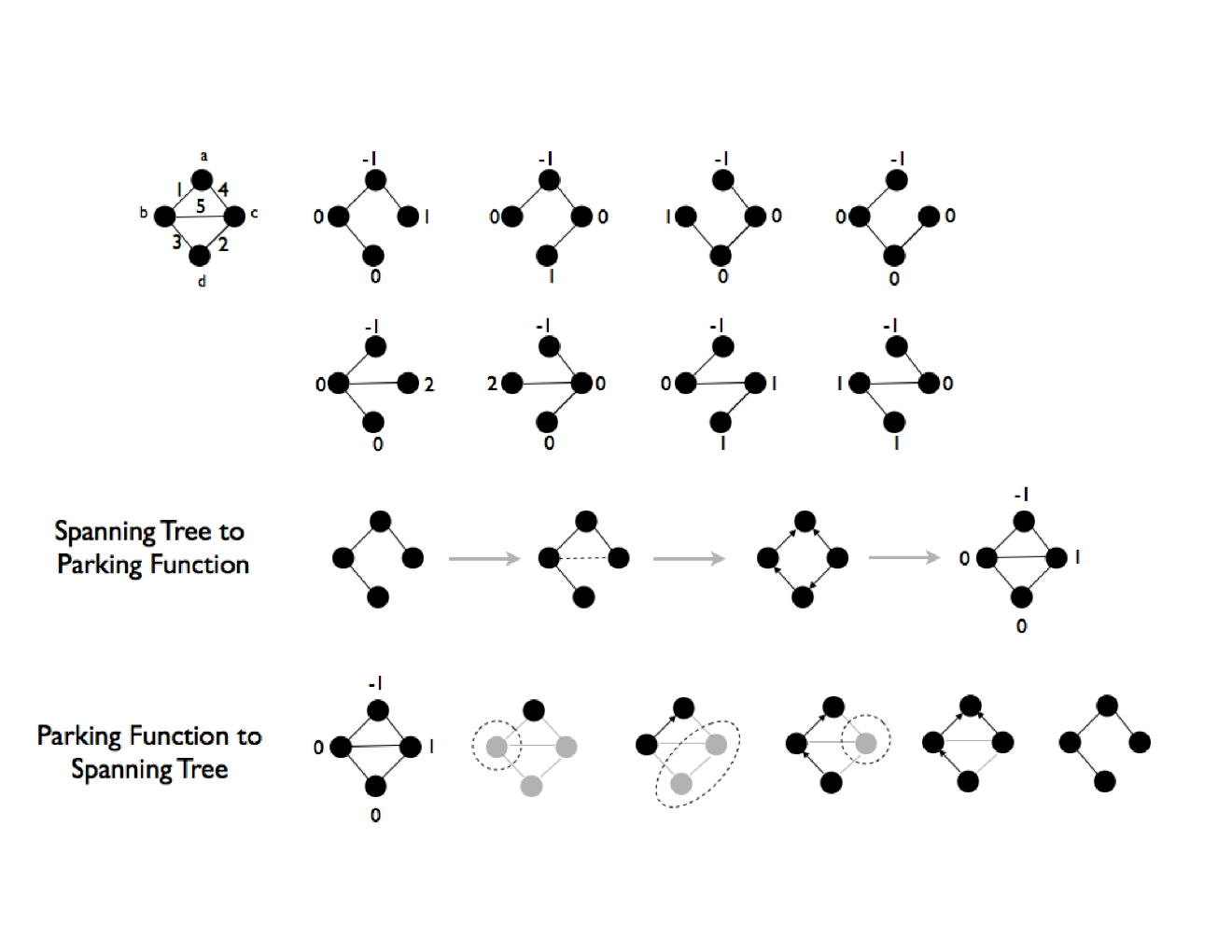
We end this section by using the relation between parking function and orientations to prove a property about the poset formed by parking functions. Recall given two parking functions $f$ and $g$ , we say that $f\prec g$ iff $f(v)\leq g(v)$ for all vertices $v\in V$ . Also recall the parking function $f\wedge g$ defined as $(f\wedge g)(v):=\min(f(v),g(v))$ . Finally, recall ${\rm dom}(f):=\{g\mbox{ a parking function }:g\prec f\}$ .

Lemma 4.12.

Given a non-maximum parking function $g$ , let $F_{g}$ be the set of maximum parking functions that dominate $g$ . Then, $g=\bigwedge_{f\in F_{g}}f$ .

Proof.

It is clear that any non-maximum parking function $g$ is dominated by the meet of all maximum parking functions which dominate it. The lemma claims that it is in fact exactly equal to the meet. To show this, it suffices to show that for any $v$ , there exists a parking function $f$ such that $f(v)=g(v)$ , $f(u)\geq g(u)$ for all $u\in V$ and $f(w)>g(w)$ for exactly one vertex $w\neq v$ . Continuing this process, we get a maximum parking function which agrees with $g$ on $v$ . Since this is true for all $v$ , we are done.

To prove the above, note that from the bijection between parking functions and spanning trees, we see that any parking function $g$ uniquely corresponds to a mixed orientation of the edges of $G$ , where a mixed orientation has some edges directed and others undirected. Moreover, the directed edges induce a DAG.

Consider the mixed orientation with respect to $g$ . Let $D$ be the DAG induced by the set of directed edges. Suppose there is an edge $(u,w)$ which is not oriented where $u$ and $w$ are distinct from $v$ ; then in $D$ if there is a directed path from $u$ to $w$ , orient the edge from $u$ to $w$ , else orient the edge from $w$ to $u$ . if there is no path either way, orient in any of the two ways. We still have a mixed orientation where the directed edges are acyclic. Moreover, this increases the value of parking function on exactly one of $u$ or $w$ , and keeps the value the same everywhere else.

Thus, the non-trivial case is when the only undirected edges are incident on $v$ . Let $(u,v)$ be such an edge. Note that we do not want to increase $g(v)$ , that is, we want to orient $(u,v)$ without increasing $v$ ’s out-degree. In other words, we want to orient it from $u$ to $v$ . This is a problem if and only if there is a path from $v$ to $u$ in $D$ . If so, consider the longest such a path $P=(v,w,\ldots,u)$ , where $w$ is the neighbor of $v$ on $P$ .

Note that apart from the edge $(v,w)$ , there is no path from $v$ to $w$ . If there were such a path, it can not use vertices from $P$ , for $w$ “dominates” (in the DAG) all vertices in $P$ other than $v$ . Thus, the path from $v$ to $w$ must use “new” vertices making $P$ longer, and thus providing a contradiction.

Therefore, we can flip $(v,w)$ to $(w,v)$ and not create any cycles. That is, the operation to get $f$ is to flip $(v,w)$ to $(w,v)$ and orient $(v,u)$ from $v$ to $u$ . This only increases $g(w)$ but keeps everything else the same. ∎

5. Product Graphs and $Q_{n}$ -Parking Functions

Given two graphs $G_{1}$ and $G_{2}$ , there is a standard notion of the Cartesian product $G_{1}\Box G_{2}$ of the two graphs. Given a $G_{1}$ -parking function and a $G_{2}$ -parking function, we define below a $G_{1}\Box G_{2}$ -parking function in a natural way that is symmetric in $G_{1}$ and $G_{2}$ .

Definition 5.1.

Given $G_{1}=(V_{1},E_{1})$ and $G_{2}=(V_{2},E_{2})$ , the Cartesian product graph $G_{1}\Box G_{2}=(V,E)$ is defined on the vertex set $V=V_{1}\times V_{2}$ , using the edge set $E=E^{\prime}\cup E^{\prime\prime}$ , where $E^{\prime}=\bigl\{\{(u_{1},v),(u_{2},v)\}:\{u_{1},u_{2}\}\in E_{1}\mbox{ and }v\in V_{2}\bigr\}$ , and $E^{\prime\prime}=\bigl\{\{(u,v_{1}),(u,v_{2})\}:\{v_{1},v_{2}\}\in E_{2}\mbox{ and }u\in V_{1}\bigr\}\,$ .

It is easy to see from the definition that the number of vertices in $G_{1}\Box G_{2}$ is $|V_{1}|\,|V_{2}|$ , and that the number of edges is $|V(G_{2})|\,|E(G_{1})|+|V(G_{1})|\,|E(G_{2})|$ .

5.1. Parking functions on Product graphs

While it seems hard to characterize parking functions on $G_{1}\Box G_{2}$ , by simply knowing those on $G_{1}$ and on $G_{2}$ , the following result gives an explicit way to construct a particular family of maximum parking functions on product graphs.

Proposition 5.1.

Let $f_{1}\in{\mathcal{P}}(G_{1};q_{1})$ and $f_{2}\in{\mathcal{P}}(G_{2};q_{2})$ . Then $f_{1}\Box f_{2}\in{\mathcal{P}}\bigl(G_{1}\Box G_{2};(q_{1},q_{2})\bigr)$ , where $f_{1}\Box f_{2}(u,v)=f_{1}(u)+f_{2}(v)+1$ , whenever $u\in G_{1}$ and $v\in G_{2}$ .

Further, if $f_{1}$ and $f_{2}$ are maximum parking functions, then $f_{1}\Box f_{2}$ is a maximum parking function.

Proof. Let $f=f_{1}\Box f_{2}$ , $G=G_{1}\Box G_{2}$ , and $q=(q_{1},q_{2})$ . To show that $f\in{\mathcal{P}}(G,q)$ , once again we make crucial use of Dhar’s marking algorithm; in particular, we will make use of the order in which the vertices of $G_{1}$ (and $G_{2}$ ) are marked in verifying that $f_{1}\in{\mathcal{P}}(G_{1},q_{1})$ (and $f_{2}\in{\mathcal{P}}(G_{2},q_{2})$ , respectively). Using these in turn, we order the vertices in $G_{1}\Box G_{2}$ : let $(u^{\prime},v^{\prime})<_{\Box}(u,v)$ , if $u^{\prime}$ is marked before $u$ in $G_{1}$ , or if $u=u^{\prime}$ and $v^{\prime}$ is marked before $v$ in $G_{2}$ . We now prove that $f$ is a valid parking function, by showing that the vertices of $G_{1}\Box G_{2}$ can be marked, using Dhar, in precisely the order given by $<_{\Box}$ . We begin by noting that $f(q)=f(q_{1},q_{2})=f_{1}(q_{1})+f_{2}(q_{2})+1=-1$ . Now consider the vertices of $G$ inductively, using the order given by $<_{\Box}$ . By the time the vertex $(u,v)$ is considered, observe that there are at least $f(u)+f(v)+2$ neighbors of $(u,v)$ that have already been marked, since they precede $(u,v)$ in $<_{\Box}$ : indeed, at least $f(u)+1$ neighbors of the form $(u^{\prime},v)$ have been marked, (since the graph induced by fixing the second coordinate $v$ is simply $G_{1}$ ), and similarly at least $f(v)+1$ neighbors of the form $(u,v^{\prime})$ have also been marked. Thus $(u,v)$ can be assigned the value $f(u,v)=f(u)+f(v)+1$ , and hence $f$ is a $G$ -parking function.

Now, suppose that $f_{1}$ and $f_{2}$ are maximum $G_{1}$ - and $G_{2}$ -parking functions respectively. Then, we must show that $f$ achieves the genus of ${\bf g}(G)$ minus one. This is easy to verify:

$\displaystyle\\|f_{1}\Box f_{2}\\|$	$\displaystyle=$	$\displaystyle\|V(G_{2})\|\,\\|f_{1}\\|+\|V(G_{1})\|\,\\|f_{2}\\|+\|V(G_{1})\|\,\|V(G_{2})\|$
	$\displaystyle=$	$\displaystyle\|V(G_{2})\|\,\|E(G_{1})\|+\|V(G_{1})\|\,\|E(G_{2})\|-\|V(G_{1})\|\,\|V(G_{2})\|$
	$\displaystyle=$	$\displaystyle\|E(G_{1}\Box G_{2})\|-\|V(G_{1}\Box G_{2})\|={\bf g}(G_{1}\Box G_{2})-1.\vskip-56.9055pt$

5.2. $Q_{n}$ -Parking Functions

A quintessential product graph is the $n$ -dimensional cube $Q_{n}$ , obtained by taking the product of an edge $Q_{1}$ with itself $n$ times. For the purpose of this section, for integer $n\geq 1$ , we also view the $n$ -cube $Q_{n}$ as the graph on $2^{n}$ vertices, which may conveniently be labeled by the $2^{n}$ binary vectors of length $n$ , and with edges between vertices whose Hamming distance is one. We are interested in understanding the parking functions on $Q_{n}$ with respect to the vertex $q=(0,0,\ldots,0)$ .

Definition 5.2.

For $n=1$ , the unique parking function $f=f^{1}$ on $Q_{1}$ is canonical. For $n>1$ , the parking function $f^{n}=\underbrace{f\Box f\Box\cdots\Box f}_{n\text{ times}}$ , obtained using the product graph construction, is defined as the canonical $Q_{n}$ -parking function. Further, if a $Q_{n}$ -parking function $g$ is such that there exists a bijection $\phi:V(Q_{n}){\rightarrow}V(Q_{n})$ such that $f(v)=g(\phi(v))$ for all $v\in V(Q_{n})$ , then we say that $g$ is semi-canonical.

Note that by Proposition 5.1, the canonical $Q_{n}$ -parking function is a maximum parking function, and hence the semi-canonical one is also a maximum.

Example 5.1.

Not all maximal $Q_{n}$ -parking functions are semi-canonical. For instance, consider the $Q_{3}$ -parking function $f$ such that $f(000)=-1,f(001)=1,f(010)=0,f(100)=2,f(011)=0,f(101)=0,f(110)=0,f(111)=2$ . It is easy to verify that $f$ is a $Q_{3}$ -parking function, but $f$ is not semi-canonical. Since, $\|f\|=4=|E|-|V|$ , $f$ is maximum (and thus maximal).

Recall the partial order on parking functions, and the notion of ${\rm dom}(f)=\{g\in{\mathcal{P}}(G,q):g\prec f\}$ , for a parking function $f\in{\mathcal{P}}(G,q)$ .

Theorem 5.2.

Let $f^{n}$ denote the canonical $Q_{n}$ -parking function. Then $f^{n}(v)={\rm wgt}(v)-1$ , where ${\rm wgt}(v)$ is the Hamming weight (the number of 1’s in the binary representation) of the vertex $v\in V(Q_{n})$ . Consequently, if $f$ is semi-canonical, then

\left|{\rm dom}(f)\right|=\prod_{k=2}^{n}k^{n\choose k}.

Proof. The proof is by an easy induction on $n\in{\mathbb{Z}}^{+}$ . The base case is clear, since $f^{1}$ takes the values $-1,0$ . For the induction step, for $n\geq 1$ , write $f^{n+1}=f^{n}\Box f^{1}$ , which by Proposition 5.1 implies that, for $u\in V(Q_{n})$ and $v\in V(Q_{1})=\{0,1\}$ ,

f^{n+1}(u,v)=f^{n}(u)+f^{1}(v)+1\,.

Thus for $0\leq k\leq n$ , the value $k$ can be obtained in $f^{n+1}$ either by taking a $k$ from $f^{n}$ and adding a zero to it (through, $f^{1}(0)+1=-1+1$ ), or by taking a $k-1$ from $f^{n}$ and adding a one to it (through, $f^{1}(1)=0+1$ ). By the induction hypothesis, the number of $k$ ’s is

{n\choose k}+{n\choose k-1}={n+1\choose k}\,,

completing the induction step. Also note that, by definition, a semi-canonical parking function also has the same distribution of integers.

To complete the proof of the theorem, recall by Proposition 2.2, that for any $v\in V(Q_{n})\backslash\{q\}$ , if $f(v)=k$ for $k\in{\mathbb{Z}}_{\geq 1}$ , then for $g\prec f$ , we may have $g(v)=0,1,\ldots k$ ; this implies that there are $k+1$ possible values for such a $g$ with respect to $v$ . Since $0\leq k\leq n$ and each value in the range of $f$ is independent with respect to obtaining a dominated function $g$ , we have that

\left|{\rm dom}(f)\right|=\prod_{k=2}^{n}k^{n\choose k}.

Remark 5.1.

Note that it can directly be seen that $f$ is a $Q_{n}$ -parking function, when $f$ is defined as $f(v)={\rm wgt}(v)-1$ . Using Dhar’s algorithm, starting with $q=(0,0,\ldots,0)$ , we may proceed by marking vertices level by level (in the Boolean lattice ): Every vertex $v$ in level $k$ has precisely $k$ down-neighbors in level $k-1$ , and they have all been marked, so $v$ can be marked and given value $k-1$ . Thus there are precisely ${n\choose k}$ vertices which obtain the value $k-1$ , in such a canonical parking function on $Q_{n}$ .

Example 5.2.

Note that not every semi-canonical parking function is canonical – in satisfying the level by level property described in Remark 5.1. For instance, consider the $Q_{3}$ -parking function $f$ such that $f(000)=-1,\ f(010)=f(100)=f(101)=0,\ f(001)=f(011)=f(111)=1$ , and $f(110)=2$ . It is easy to check that $f$ is a $Q_{3}$ -parking function, semi-canonical, but not canonical – since, for example, the value 2 is adjacent to a 0.

We hope the above remarks and examples indicate the difficulty in understanding the maximum parking functions on even a highly structured, symmetric graph such as the $n$ -cube. As far as we know, the number of maximum parking functions of $Q_{n}$ is known only for $n\leq 4$ . For $n=2,3$ , and 4, this number is 3, 133, and 3040575, respectively.

6. Diffuse states and acyclic orientations

As mentioned in the introduction, in the context of chip-firing, the following notion was introduced in [25].

Definition 6.1.

Given a connected graph $G$ , a function $s:G\to{\mathbb{Z}}^{+}$ is called a diffuse state if for every induced subgraph $G[A]=(A,E(A))\subseteq G$ , there exists some $u\in A$ such that $\deg(u)|_{A}\leq s(u)$ . Further, let $\|s\|:=\sum_{v}s(v)$ .

Note the (complementary) similarity with the definition of a parking function, by observing that $\deg(u)|_{A}\leq s(u)$ is equivalent to $\deg(u)-s(u)\leq\deg(u)|_{A^{c}}$ . However, we have no special vertex such as $q$ . For chip-firing purposes, $s(v)$ may be thought of as the number of chips on $v$ , thus $\|s\|$ denotes the total number of chips in the graph.

First consider the following algorithm which constructs an acyclic orientation, by using a given diffuse state $s$ with $|E(G)|$ chips.

Step 1. Since $s$ is diffuse, we may find a vertex $v$ such that $\deg(v)|_{G}=\deg(v)\leq s(v)$ .

Step 2. Orient all of the edges incident to $v$ outward; delete $v$ and its incident edges.

Step 3. The resulting graph is diffuse since it is a subgraph of $G$ ; so we may repeat Steps 1-2 until all edges of the graph are oriented.

Note that this process gives an acyclic orientation since we cannot orient edges into a vertex which has out edges since this vertex has been deleted from the graph.

Lemma 6.1.

If $s$ is a diffuse state on graph $G$ with $\|s\|=|E(G)|$ , then there is a vertex $v$ with $s(v)=0$ . For every diffuse state $s$ , the set $\{v:s(v)=0\}$ is an independent set in $G$ .

Proof.

The above algorithm which repeatedly removes vertices, removes at least as many chips as the edges at each step. Before the last vertex, all edges (hence all $|E(G)|$ chips) must have been removed, which means that the last vertex can has zero chips. For the second part, if $s(u)=s(v)=0$ , and $u,v\in E(G)$ then the set $A=\{u,v\}$ violates the diffuse property.

With a similar proof, it can also be shown that there exists a vertex $w$ such that $s(w)=\deg(w)$ , under the hypothesis of the above lemma.

Theorem 6.2.

There is a bijection between the set ${\rm D}(G)$ of diffuse states with $|E(G)|$ chips and the set ${\rm AO}(G)$ of acyclic orientations of a connected graph $G$ .

Proof.

Let $E(G)=m$ . The proof is based on two injections between the sets, going in each direction. First, given an acyclic orientation ${\mathcal{O}}\in{\rm AO}(G)$ , define the nonnegative function $s=s_{\mathcal{O}}$ by letting $s(v)$ be the out-degree of $v$ in the orientation ${\mathcal{O}}$ . Clearly, the mapping is one-one, since the out-degree sequence uniquely determines an acyclic orientation; also $\|s\|=m$ , since the sum of out-degrees equals the number of edges. To see that $s$ is diffuse, simply observe that, each induced subgraph $G[A]\subseteq G$ has a (local) source $y\in A$ when restricted to the acyclic orientation induced on $A$ ; such a source $y$ satisfies $s(y)\geq\deg(y)|_{A}$ , since the out-degree of $y$ is at least the degree $\deg(y)|_{A}$ .

For an injection in the other direction, we make use Lemma 6.1. Given a diffuse state $s$ with $m$ chips, we construct an acyclic orientation, by constructing a DAG: Lemma 6.1 guarantees the existence of sink(s); so we construct the orientation, by (i) repeatedly removing the current set of sinks, and (ii) subtracting a chip from each in-neighbor of a removed sink. It is easy to see that the updated function $s$ at each step is still a diffuse state on the remaining graph. Note that this construction is one-one: for $s,s^{\prime}$ different diffuse states, simply consider the first time the current sets of sinks (in the DAGs) differ, when we start with $s$ versus $s^{\prime}$ ; since the underlying graph is the same, there must be such a time whenever $s\neq s^{\prime}$ .

Remark 6.1.

Thanks again to an anonymous referee of [6], we learnt the following: that diffuse states are also in 1-1 correspondence with the critical configurations of the chip-firing game of Björner-Lovász-Shor [11], and that the first part of the above proof appears as Theorem 3.3, part (b) in [11]. In addition, it is easy to go between the above theorem and Theorem 3.1: simply add a new vertex $q$ adjacent to every vertex in $G$ and obtain a new graph $\hat{G}$ ; then $\hat{G}$ -parking functions (with respect to $q$ , say) correspond to diffuse states in $G$ , and acyclic orientations with a unique source at $q$ in $\hat{G}$ correspond to acyclic orientations of $G$ .

7. Concluding Remarks

Soon after the completion of this work, Igor Pak kindly pointed us to the work of Olivier Bernardi [7], where bijective proofs are derived for interpretations of each of the evaluations of the Tutte polynomial ${\mathcal{T}}_{G}(x,y)$ , for $0\leq x,y\leq 2$ , in terms of orientations. A key to this seems to be a nice combinatorial embedding of (the edges of) the graph and a rewriting of the Tutte polynomial using notions of internal and external embedding activity.

In addition to the questions mentioned in the previous sections, several challenging problems remain open. Given an arbitrary graph $G$ , it is a classical open problem in the topic of Markov chain Monte Carlo (MCMC) algorithms [26], to efficiently generate an acyclic orientation uniformly at random from the set of all such orientations. Due to the observations above, a closely related problem would be to generate at random an acyclic orientation with a uniquely identified sink (or source), or equivalently, to sample uniformly from the set of safe spanning trees of $G$ . The MCMC technique suggests the following natural approach to this problem: it is well known (see for example, [18, 19]) that the so-called bases exchange walk provides an efficient way to sample uniformly from the set of all spanning trees of a given graph $G$ . However it remains to be seen whether (and how) restricting such a random walk to the set of safe trees affects the mixing time of the walk – the time by which the walk converges to its steady state distribution, uniform on the set of safe trees. Given that the exact enumeration of the number of safe trees of $Q_{n}$ is also open, an interesting first step might be to analyze such a walk on the trees of $Q_{n}$ .

Independent of the above approach, other ways of providing asymptotically accurate estimates, for large $n$ , of the number (or even the logarithm of the number) of maximum parking functions on $Q_{n}$ , remains interesting and presumably a challenging exercise.

Acknowledgements. The authors thank Matt Baker for introducing them to $G$ -parking functions and for helpful discussions. The authors also thank Adam Marcus for helpful discussions, and Herb Wilf for providing the chromatic polynomial of $Q_{4}$ , which identified the number of maximum parking functions of $Q_{4}$ . The authors are grateful to the anonymous referees for making several critical remarks which helped improve the presentation here. The present work originated from a summer 2007 REU, supported by an REU supplement to the last author’s NSF grant DMS-0701043.

References

[1] P. Bak, C. Tang, and K. Wiesenfeld, Self-organized criticality: an explanation of the $1/f$ noise, Phys. Rev. Lett. 59 (1987), 381–384.
[2] M. Baker and S. Norine, Riemann-Roch and Abel-Jacobi Theory on a Finite Graph, Advances in Mathematics 215 (2007), pp. 766–788.
[3] M. Baker, Personal Communication.
[4] R. Bari, A combinatorial approach to graphical polynomials and spanning subgraphs, Topics in graph theory (New York, 1977), pp. 21–29, Ann. New York Acad. Sci., 328, New York Acad. Sci., New York, 1979.
[5] R. Bari, Chromatic Polynomials and the internal and external activities of Tutte, Graph theory and related topics, pp. 41–52, Academic Press (1979), New York.
[6] B. Benson and P. Tetali, Parking Functions and Acyclic Orientations of Graphs, math arxiv 2008; available at http://arxiv.org/abs/0801.1114
[7] O. Bernardi, Tutte Polynomial, Subgraphs Orientations, and Sandpile Model: New Connections via Embeddings, Electronic J. of Combinatorics, 15 (2008), R109 (52 pages).
[8] N. L. Biggs, Chip-Firing and the Critical Group of a Graph, J. of Algebraic Comb. 9 (1999), pp. 25–45.
[9] N.L. Biggs, The Tutte polynomial as a Growth function, J. of Algebraic Comb. 10 (1999), pp. 115–133.
[10] N.L. Biggs and P. Winkler, Chip-firing and the chromatic polynomial, Research report LSE-CDAM-97-03, CDAM, 1997.
[11] A. Björner, L. Lovász and P. Shor, Chip-firing games on graphs, Euro. J. Combin. 12 (1991), 283–291.
[12] A. Blass and B. Sagan, Bijective proofs of two broken circuit theorems, J. Graph Theory 10 (1986), pp. 15–21.
[13] D. Chebikin and P. Pylyavskyy, A family of bijections between $G$ -parking functions and spanning trees, Jour. Combin. Theory (Series A) 110 (2005), pp. 31–41.
[14] R. Cori, Y. Le Borgne, The sand-pile model and Tutte polynomials, Adv. Appl. Math. 30 (2003), pp. 44–52.
[15] R. Cori and D. Rossin, On the sandpile group of dual graphs, Euro. J. Combin. 21 (2000), pp. 447–559.
[16] R. Cori, D. Rossin, B. Salvy, Polynomial ideals for sandpiles and their Grobner bases, Theor. Comp. Sci. 276 (2002), pp. 1–15.
[17] D. Dhar, Self-organised critical state of the sandpile automaton models, Physical Review Letters 64 (1990), pp. 1613–1616.
[18] T. Feder and M. Mihail, Balanced Matroids, Proc. of the 24th Annual ACM Symp. on Theory of Computing (1992), 26–38.
[19] J. Fehrenbach and L. Rüschendorf, Analysis of Markov chain algorithms on spanning trees, rooted forests, and connected subgraphs, Appl. Math. (Warsaw) 32 (2005), 341–365.
[20] A. Gabrielov, Abelian Avalanches and Tutte Polynomials, Physica A 195 (1993), 253–274.
[21] D. D. Gebhard and B. E. Sagan, Sinks in Acyclic Orientations of Graphs, Jour. of Combin. Th. (Series B) 80 (1999), pp. 130–146.
[22] E. Gioan and M. Las Vergnas, Activity preserving bijections between spanning trees and orientations in graphs, Discrete Math. 298 (2005), pp. 169–188.
[23] C. Godsil and G. Royle, Algebraic Graph Theory, Springer-Verlag GTM Vol. 207 (2001), New York.
[24] C. Greene and T. Zaslavsky, On the Interpretation of Whitney Numbers through Arrangements of Hyperplanes, Zonotopes, Non-Radon Partitions, and Orientations, Trans. Amer. Math. Soc. 280 (1983), pp. 97–126.
[25] J. Jeffs and S. Seager, The chip firing game on $n$ -cycles, Graphs Combin., 11 (1995), pp. 59–67.
[26] M. Jerrum and A. Sinclair, The Markov chain Monte Carlo method: an approach to approximate counting and integration. In D. Hochbaum (Ed.), Approximation Algorithms for NP-hard problems, PWS Publishing (1996), pp. 482–520.
[27] R. Kenyon and P. Winkler, Branched Polymers, Amer. Math. Monthly, to appear.
[28] M. Las Vergnas, A correspondence between spanning trees and orientations in graphs, in: B. Bollobas (Ed.), Graph Theory and Combinatorics, Proceedings of Cambridge Combinatorial Conference in Honour of P. Erdos, Cambridge, 1983, Academic Press, London, 1984, pp. 233–238.
[29] C. M. Lopez, Chip Firing and the Tutte Polynomial, Annals of Combinatorics 1 (1997), pp. 253–259.
[30] J. Plautz and R. Calderer, $G$ -Parking Functions and the Tutte Polynomial, Preprint.
[31] A. Postnikov and B. Shapiro, Trees, parking functions, syzygies, and deformations of monomial ideals, Transactions of the American Mathematical Society 356 (2004), pp. 3109–3142.
[32] R. Stanley, Enumerative Combinatorics, Vol. II, Cambridge Studies in Advanced Mathematics Vol. 62, Cambridge University Press (1999), Cambridge.
[33] W.T. Tutte, A Contribution to the Theory of Chromatic Polynomials, Canad. J. Math. 6 (1954), pp. 80–91.
[34] D.J.A. Welsh, Complexity: Knots, Colourings, and Counting, London Math Soc. Lecture Note Series Vol. 186, Cambridge University Press (1993), Cambridge.
[35] H. Whitney, A Logical Expansion in Mathematics, Bull. Amer. Math. Soc. 38 (1932), pp. 572–579.

$\displaystyle\|{\mathcal{P}}(G,q)\|$	$\displaystyle=$	$\displaystyle\|\cup_{i=1}^{k}{\rm dom}(g_{i})\|$
	$\displaystyle=$	$\displaystyle\sum_{i}\|{\rm dom}(g_{i})\|-\sum_{1\leq i<j\leq k}\|{\rm dom}(g_{i})\cap{\rm dom}(g_{j})\|+\cdots$
		$\displaystyle+(-1)^{k}\|{\rm dom}(g_{1})\cap{\rm dom}(g_{2})\cap\cdots\cap{\rm dom}(g_{k})\|$
	$\displaystyle=$	$\displaystyle\sum_{i}\|{\rm dom}(g_{i})\|-\sum_{1\leq i<j\leq k}\|{\rm dom}(g_{i}\wedge g_{j})\|+\cdots+(-1)^{k}\|{\rm dom}(g_{1}\wedge g_{2}\wedge\cdots\wedge g_{k})\|\,,$

$\displaystyle\\|f_{1}\Box f_{2}\\|$	$\displaystyle=$	$\displaystyle\|V(G_{2})\|\,\\|f_{1}\\|+\|V(G_{1})\|\,\\|f_{2}\\|+\|V(G_{1})\|\,\|V(G_{2})\|$
	$\displaystyle=$	$\displaystyle\|V(G_{2})\|\,\|E(G_{1})\|+\|V(G_{1})\|\,\|E(G_{2})\|-\|V(G_{1})\|\,\|V(G_{2})\|$
	$\displaystyle=$	$\displaystyle\|E(G_{1}\Box G_{2})\|-\|V(G_{1}\Box G_{2})\|={\bf g}(G_{1}\Box G_{2})-1.\vskip-56.9055pt$

GG-Parking Functions, Acyclic Orientations and Spanning Trees

Abstract.

1. Introduction

2. GG-Parking Functions and Dhar’s Burn Criteria

Definition 2.1.

Remark 2.1.

Proposition 2.1.

Definition 2.2.

Proposition 2.2.

Proposition 2.3.

3. Maximal GG-Parking Functions and Acyclic Orientations with a Unique Source

Theorem 3.1.

Remark 3.1.

Corollary 3.2.

Proof.

Corollary 3.3.

Theorem 3.4.

Corollary 3.5.

Corollary 3.6.

4. Bijections of Maximal GG-parking Functions

Definition 4.1.

Theorem 4.1.

Proof.

Remark 4.1.

4.1. Bijection between Acyclic Orientations with Unique Sink and Safe Trees

Theorem 4.2.

Lemma 4.3.

Proof.

Lemma 4.4.

Proof.

Remark 4.2.

4.2. Extension to a bijection of GG-Parking Functions and Spanning Trees

Claim 4.5.

Proof.

Theorem 4.6.

Proposition 4.7.

Proof.

Claim 4.8.

Proof.

Claim 4.9.

Proof.

Lemma 4.10.

Proof.

Lemma 4.11.

Proof.

Lemma 4.12.

Proof.

5. Product Graphs and QnQ_{n}-Parking Functions

Definition 5.1.

5.1. Parking functions on Product graphs

Proposition 5.1.

5.2. QnQ_{n}-Parking Functions

Definition 5.2.

Example 5.1.

Theorem 5.2.

Remark 5.1.

Example 5.2.

6. Diffuse states and acyclic orientations

Definition 6.1.

Lemma 6.1.

Proof.

Theorem 6.2.

Proof.

Remark 6.1.

7. Concluding Remarks

References

$G$ -Parking Functions, Acyclic Orientations and Spanning Trees

2. $G$ -Parking Functions and Dhar’s Burn Criteria

3. Maximal $G$ -Parking Functions and Acyclic Orientations with a Unique Source

4. Bijections of Maximal $G$ -parking Functions

4.2. Extension to a bijection of $G$ -Parking Functions and Spanning Trees

5. Product Graphs and $Q_{n}$ -Parking Functions

5.2. $Q_{n}$ -Parking Functions