Elliptic integral evaluations of Bessel moments

David H. Bailey ^†^†thanks: Lawrence Berkeley National Laboratory, Berkeley, CA 94720, USA, dhbailey@lbl.gov. Supported in part by the Director, Office of Computational and Technology Research, Division of Mathematical, Information and Computational Sciences, U.S. Department of Energy, under contract number DE-AC02-05CH11231. Jonathan M. Borwein ^†^†thanks: Faculty of Computer Science, Dalhousie University, Halifax, NS, B3H 2W5, Canada, jborwein@cs.dal.ca. Supported in part by NSERC and the Canada Research Chair Programme. David Broadhurst ^†^†thanks: Department of Physics and Astronomy, The Open University, Milton Keynes, MK7 6AA, United Kingdom, D.Broadhurst@open.ac.uk. M.L. Glasser ^†^†thanks: Department of Physics, Clarkson University, Potsdam, NY 13699-5820, USA, laryg@clarkson.edu.

August 24, 2026

Abstract

We record what is known about the closed forms for various Bessel function moments arising in quantum field theory, condensed matter theory and other parts of mathematical physics. More generally, we develop formulae for integrals of products of six or fewer Bessel functions. In consequence, we are able to discover and prove closed forms for $c_{n,k}:=\int_{0}^{\infty}t^{k}K_{0}^{n}(t)\,{\rm d}t$ with integers $n=1,2,3,4$ and $k\geq 0$ , obtaining new results for the even moments $c_{3,2k}$ and $c_{4,2k}$ . We also derive new closed forms for the odd moments $s_{n,2k+1}:=\int_{0}^{\infty}t^{2k+1}I_{0}(t)\,K_{0}^{n-1}(t)\,{\rm d}t$ with $n=3,4$ and for $t_{n,2k+1}:=\int_{0}^{\infty}t^{2k+1}I_{0}^{2}(t)\,K_{0}^{n-2}(t)\,{\rm d}t$ with $n=5$ , relating the latter to Green functions on hexagonal, diamond and cubic lattices. We conjecture the values of $s_{5,2k+1}$ , make substantial progress on the evaluation of $c_{5,2k+1}$ , $s_{6,2k+1}$ and $t_{6,2k+1}$ and report more limited progress regarding $c_{5,2k}$ , $c_{6,2k+1}$ and $c_{6,2k}$ .

In the process, we obtain 8 conjectural evaluations, each of which has been checked to 1200 decimal places. One of these lies deep in 4-dimensional quantum field theory and two are probably provable by delicate combinatorics. There remains a hard core of five conjectures whose proofs would be most instructive, to mathematicians and physicists alike.

1 Introduction

We give representations of the vacuum [35, 56] and sunrise [30, 40, 41] diagrams

	$\displaystyle V_{n}(a_{1},\ldots,a_{n})$	$\displaystyle:=$	$\displaystyle\int_{0}^{\infty}t\left(\prod_{j=1}^{n}K_{0}(a_{j}t)\right)\,{\rm d}t$		(1)
	$\displaystyle S_{n+1}(a_{1},\ldots,a_{n},w)$	$\displaystyle:=$	$\displaystyle\int_{0}^{\infty}t\left(\prod_{j=1}^{n}K_{0}(a_{j}t)\right)J_{0}(wt)\,{\rm d}t$		(2)

where all the arguments of $V_{n}$ and all but the last argument of $S_{n+1}$ are real and positive. Here and below $I_{0},J_{0}$ and $K_{0}$ are the conventional Bessel functions of order zero as in [1, Chapter 15]. These integrals occur in quantum field theories in two spacetime dimensions, where we do not need to regularize ultraviolet divergences. Numbers generated by them are expected to occur in the finite parts of integrals from Feynman diagrams in four spacetime dimensions. To be concrete, we illustrate $V_{3}$ and $S_{4}$ as follows:

By casting Bessel’s differential equation in the form

\left(\frac{1}{a}+\frac{{\rm d}}{{\rm d}a}\right)\frac{{\rm d}}{{\rm d}a}\,K_{0}(at)=t^{2}K_{0}(at)

and applying the corresponding differential operator to (1), we may increase the exponent of $t$ in the integrand by steps of 2. But to obtain even powers of $t$ , we need to start with

\overline{V}_{n}(a_{1},\ldots,a_{n}):=\int_{0}^{\infty}\left(\prod_{j=1}^{n}K_{0}(a_{j}t)\right)\,{\rm d}t

(3)

which plays no obvious role in quantum field theory. To evaluate the latter form, we found it useful to regard the Fourier transform

\overline{S}_{n+1}(a_{1},\ldots,a_{n},w):=\frac{1}{\pi}\int_{0}^{\infty}\left(\prod_{j=1}^{n}K_{0}(a_{j}t)\right)\cos(wt)\,{\rm d}t\

(4)

as an analogue of (2).

We shall be especially interested in the moments

c_{n,k}:=\int_{0}^{\infty}t^{k}K_{0}^{n}(t)\,{\rm d}t

(5)

for integers $n\geq 1$ and $k\geq 0$ , as studied in [8, 10] and [26, 60].

In [10] these moments arose in the study of Ising-type integrals

C_{n,k}=\frac{1}{n!}\int_{0}^{\infty}\cdots\int_{0}^{\infty}\frac{{\rm d}x_{1}\ {\rm d}x_{2}\cdots\ {\rm d}x_{n}}{(\cosh x_{1}+\dots+\cosh x_{n})^{k+1}}

which are linked by

C_{n,k}=\frac{2^{n}}{n!\,k!}\,c_{n,k}\,.

(6)

In [26, 60] it is proven that for fixed $n$ these moments satisfy a linear recursion for which a simple algorithm exists with coefficients polynomial in $k$ . For example, for $n=1$ and $2$ one easily obtains the closed forms

c_{1,k}=2^{k-1}\,\Gamma^{2}\left(\frac{k+1}{2}\right)\,\mbox{ and }\,c_{2,k}=\frac{\sqrt{\pi}\;\Gamma^{3}\left(\frac{k+1}{2}\right)}{4\,\Gamma\left(\frac{k}{2}+1\right)}

(7)

and for $n=3$ and $4$ we obtain the recursions

	$\displaystyle(k+1)^{4}c_{3,k}-2(5k^{2}+20k+21)c_{3,k+2}+9c_{3,k+4}$	$\displaystyle=$	$\displaystyle 0$		(8)
	$\displaystyle(k+1)^{5}c_{4,k}-4(k+2)(5k^{2}+20k+23)c_{4,k+2}+64(k+3)c_{4,k+4}$	$\displaystyle=$	$\displaystyle 0\,.$		(9)

These recursion formulae may be written quite compactly as

\sum_{i=0}^{M}\,(-1)^{i}\,p_{n,i}(k+i+1)\,c_{n,k+2i}=0

(10)

where $M=\lfloor(n+1)/2\rfloor$ . For instance, for $n=5$ and $6$ , we have

\begin{array}[]{ll}p_{5,0}(x)=x^{6}&p_{6,0}(x)=x^{7}\\ p_{5,1}(x)=35x^{4}+42x^{2}+3&p_{6,1}(x)=x(56x^{4}+112x^{2}+24)\\ p_{5,2}(x)=259x^{2}+104&p_{6,2}(x)=x(784x^{2}+944)\\ p_{5,3}(x)=225&p_{6,3}(x)=2304x.\\ \end{array}

(11)

The same recursions apply to the moments

s_{n,k}:=\int_{0}^{\infty}t^{k}I_{0}(t)K_{0}^{n-1}(t)\,{\rm d}t

(12)

for integers $n\geq 3$ and $k\geq 0$ and to

t_{n,k}:=\int_{0}^{\infty}t^{k}I_{0}^{2}(t)K_{0}^{n-2}(t)\,{\rm d}t

(13)

for integers $n\geq 5$ and $k\geq 0$ .

2 Two Bessel functions

The transforms

	$\displaystyle S_{2}(a,w)$	$\displaystyle:=$	$\displaystyle\int_{0}^{\infty}t\,K_{0}(at)J_{0}(wt)\,{\rm d}t=\frac{1}{a^{2}+w^{2}}$		(14)
	$\displaystyle\overline{S}_{2}(a,w)$	$\displaystyle:=$	$\displaystyle\frac{1}{\pi}\int_{0}^{\infty}K_{0}(at)\cos(wt)\,{\rm d}t=\frac{1}{2\sqrt{a^{2}+w^{2}}}$		(15)

give $V_{1}(a)=1/a^{2}$ and $\overline{V}_{1}(a)/\pi=1/(2a)$ at $w=0$ . The distributions

	$\displaystyle\int_{0}^{\infty}vJ_{0}(vt_{1})J_{0}(vt_{2})\,{\rm d}v$	$\displaystyle=$	$\displaystyle 2\delta(t_{1}^{2}-t_{2}^{2})$		(16)
	$\displaystyle\frac{2}{\pi}\int_{0}^{\infty}\cos(vt_{1})\cos(vt_{2})\,{\rm d}v$	$\displaystyle=$	$\displaystyle\delta(t_{1}+t_{2})+\delta(t_{1}-t_{2})$		(17)

then lead to the evaluations

$\displaystyle V_{2}(a,b)$	$\displaystyle:=$	$\displaystyle\int_{0}^{\infty}t\,K_{0}(at)K_{0}(bt)\,{\rm d}t=\int_{0}^{\infty}wS_{2}(a,w)S_{2}(b,w)\,{\rm d}w$	(18)
	$\displaystyle=$	$\displaystyle\frac{\log(a/b)}{a^{2}-b^{2}}$	(18)
$\displaystyle\overline{V}_{2}(a,b)$	$\displaystyle:=$	$\displaystyle\int_{0}^{\infty}K_{0}(at)K_{0}(bt)\,{\rm d}t=2\pi\int_{0}^{\infty}\overline{S}_{2}(a,w)\overline{S}_{2}(b,w)\,{\rm d}w$	(19)
	$\displaystyle=$	$\displaystyle\frac{\pi}{a+b}\,{\bf K}\left(\frac{a-b}{a+b}\right)$	(19)

with a complete elliptic integral of the first kind,

{\bf K}(k):=\int_{0}^{\pi/2}\frac{1}{\sqrt{1-k^{2}\sin^{2}\phi}}\,{\rm d}\phi\,,

(20)

appearing in (19) and a limit intended in (18) when $a=b$ . We shall need to refer to the complementary integral ${\bf K}^{\prime}(k):={\bf K}(k^{\prime})$ , with $k^{\prime}:=\sqrt{1-k^{2}}$ . In the case $a\geq b$ , this provides a compact alternative form of (19),

\overline{V}_{2}(a,b)=\frac{\pi}{2a}\,{\bf K}^{\prime}(b/a)\,,

(21)

obtained by the Landen [3] transformation in [1, 17.3.29].

3 Three Bessel functions

We follow Källén [51, 52] by constructing $S_{3}(a,b,w)$ from its discontinuity across the cut in the $w^{2}$ plane with branch point at $w^{2}=-(a+b)^{2}$ , obtaining

S_{3}(a,b,w)=\int_{0}^{\infty}t\,K_{0}(at)K_{0}(bt)J_{0}(wt)\,{\rm d}t=\int_{a+b}^{\infty}\frac{2v\,D_{3}(a,b,v)}{v^{2}+w^{2}}\,{\rm d}v

with a discontinuity

D_{3}(a,b,c)=\frac{1}{\sqrt{(a+b+c)(a-b+c)(a+b-c)(a-b-c)}}

that is completely symmetric in its 3 arguments. The $v$ -integral is easily performed, to give

S_{3}(a,b,w)=2\,{\rm arctanh}\left(\sqrt{\frac{w^{2}+(a-b)^{2}}{w^{2}+(a+b)^{2}}}\right)D_{3}(a,b,{\rm i}w)

(22)

and in particular the on-shell value [40]

s_{3,1}=S_{3}(1,1,{\rm i}):=\int_{0}^{\infty}t\,I_{0}(t)K_{0}^{2}(t)\,{\rm d}t=L_{-3}(1)=\frac{\pi}{3\sqrt{3}}

where

L_{-3}(s):=\sum_{n=1}^{\infty}\frac{\chi_{-3}(n)}{n^{s}}=\sum_{k=0}^{\infty}\left(\frac{1}{(3k+1)^{s}}-\frac{1}{(3k+2)^{s}}\right)

is the Dirichlet $L$ -function with the real character $\chi_{-3}(n)$ given by the Legendre–Jacobi–Kronecker symbol $(D|n)$ for discriminant $D=-3$ .

Nomenclature.

We shall refer to the construction of a Feynman amplitude from its discontinuity across a cut as a dispersive calculation. Kramers [53] and Kronig [54] founded this approach in studies of the dispersion of light, in the 1920’s. In the 1950’s, the utility of dispersive methods was recognized in particle physics [45, 52, 69]. Cutkosky [31] turned them into a calculus that became a routine part of the machinery of quantum field theory. Barton [20] has given a scholarly and instructive introduction to these techniques.

3.1 The odd moments $s_{3,2k+1}$

By differentiating

S_{3}(1,1,{\rm i}x)=\frac{2\,{\rm arcsin}(x/2)}{x\sqrt{4-x^{2}}}

before setting $x=1$ , we evaluate

s_{3,3}:=\int_{0}^{\infty}t^{3}I_{0}(t)K_{0}^{2}(t)\,{\rm d}t=\left.\left(\frac{1}{x}+\frac{{\rm d}}{{\rm d}x}\right)\frac{{\rm d}S_{3}(1,1,{\rm i}x)}{{\rm d}x}\right|_{x=1}=\frac{4}{3}\,s_{3,1}

and are then able to solve the recursion relation [26, 60] for $s_{3,2k+1}$ by the closed form

s_{3,2k+1}=\frac{\pi}{3\sqrt{3}}\left(\frac{2^{k}{}k!}{3^{k}}\right)^{2}a_{k}

(23)

with integers

a_{k}=\sum_{j=0}^{k}{k\choose j}^{2}{2j\choose j}\,.

(24)

Integer sequence (24) begins

1,\,3,\,15,\,93,\,639,\,4653,\,35169,\,272835,\,2157759,\,17319837,\,140668065,\,1153462995

(25)

and is recorded¹¹ 1 See http://www.research.att.com/~ njas/sequences/A002893 . as entry A2893 of the on-line version of [66], which gives the recursion

(k+1)^{2}a_{k+1}-(10k^{2}+10k+3)a_{k}+9k^{2}a_{k-1}=0

(26)

and the generating function

I_{0}^{3}(2t)=\sum_{k=0}^{\infty}a_{k}\left(\frac{t^{k}}{k!}\right)^{2}\,.

(27)

We have verified that recursion (26) reproduces the recursion for (23), which has the same form as for the odd moments in (8). We note that integers $a_{k}$ were encountered in studies of cooperative phenomena in crystals [36] and also in studies of matrices [43] with entries 0 or 1. In [32, Prop. 2], they are related to enumeration of closed walks in a two-dimensional hexagonal lattice. They also appear in an enumeration of Feynman diagrams [61, Table 2] in quantum chromodynamics, via the constrained sum [18]

a_{k}=\sum_{p+q+r=k}\left(\frac{k!}{p!\,q!\,r!}\right)^{2}

that results from the Taylor expansion of $I_{0}^{3}$ .

It is notable that $I_{0}^{3}$ provides a generating function for moments of $I_{0}K_{0}^{2}$ . In Section 4 we shall show that $I_{0}^{4}$ generates moments of $I_{0}K_{0}^{3}$ .

3.2 The odd moments $c_{3,2k+1}$

Next, we construct

	$\displaystyle V_{3}(a,b,c)$	$\displaystyle:=$	$\displaystyle\int_{0}^{\infty}t\,K_{0}(at)K_{0}(bt)K_{0}(ct)\,{\rm d}t=\int_{0}^{\infty}wS_{3}(a,b,w)S_{2}(c,w)\,{\rm d}w$		(28)
		$\displaystyle=$	$\displaystyle\frac{L_{3}(a,b,c)+L_{3}(b,c,a)+L_{3}(c,a,b)}{4}D_{3}(a,b,c)$		(28)

with a dilogarithmic function

L_{3}(a,b,c):={\rm Li}_{2}\left(\frac{(a^{2}+b^{2}-c^{2})D_{3}(a,b,c)+1}{(a^{2}+b^{2}-c^{2})D_{3}(a,b,c)-1}\right)-{\rm Li}_{2}\left(\frac{(a^{2}+b^{2}-c^{2})D_{3}(a,b,c)-1}{(a^{2}+b^{2}-c^{2})D_{3}(a,b,c)+1}\right)

computed by Davydychev and Tausk [35]. Setting $a=b=c=1$ , we obtain

c_{3,1}=V_{3}(1,1,1)=\frac{3}{4}\,L_{-3}(2)=\frac{1}{9}\sum_{n=0}^{\infty}\left(\frac{-1}{27}\right)^{n}\sum_{k=1}^{5}\frac{v_{k}}{(6n+k)^{2}}

where the vector of coefficients $v=[9,-9,-12,-3,1]$ was discovered (and proven) in the course of investigation of 3-loop vacuum diagrams in 4 dimensions [29].

Similarly,

c_{3,3}=L_{-3}(2)-\frac{2}{3}

may be obtained by suitable differentiations of (28). Then higher moments $c_{3,2k+1}$ with $k>1$ may be obtained by using (8). Because of the mixing of $L_{-3}(2)$ with unity, we were unable to write a closed form for their rational coefficients in $c_{3,2k+1}$ .

3.3 The even moments $c_{3,2k}$

For even moments, we lack the dispersion relations [20] of quantum field theory and so fall back on the general Aufbau

\overline{S}_{m+n+1}(a_{1},\ldots a_{m},b_{1},\ldots b_{n},w)=\int_{-\infty}^{\infty}\overline{S}_{m+1}(a_{1},\ldots a_{m},v)\overline{S}_{n+1}(b_{1},\ldots b_{n},v+w)\,{\rm d}v

(29)

which follows from the distribution

\frac{1}{\pi}\int_{-\infty}^{\infty}\cos(vt_{1})\cos((v+w)t_{2})\,{\rm d}v=\delta(t_{1}+t_{2})\cos(wt_{2})+\delta(t_{1}-t_{2})\cos(wt_{2})

obtained from (17) and the expansion $\cos((v+w)t_{2})=\cos(vt_{2})\cos(wt_{2})-\sin(vt_{2})\sin(wt_{2})$ .

In particular, by setting $m=n=1$ in (29), we evaluate

\overline{S}_{3}(a,b,w):=\frac{1}{\pi}\int_{0}^{\infty}K_{0}(at)K_{0}(bt)\cos(wt)\,{\rm d}t=\int_{-\infty}^{\infty}\overline{S}_{2}(a,v)\overline{S}_{2}(b,v+w)\,{\rm d}v

as the complete elliptic integral

\overline{S}_{3}(a,b,w)=\frac{1}{4}\int_{-\infty}^{\infty}\frac{{\rm d}v}{\sqrt{(a^{2}+v^{2})(b^{2}+(v+w)^{2})}}=\frac{{\bf K}\left(\sqrt{\frac{w^{2}+(a-b)^{2}}{w^{2}+(a+b)^{2}}}\right)}{\sqrt{w^{2}+(a+b)^{2}}}

(30)

and recover the previous result (19) for $\overline{V}_{2}(a,b)=\pi\overline{S}_{3}(a,b,0)$ by setting $w=0$ .

Next, by setting $m=2$ and $n=1$ in (29), we write

\overline{S}_{4}(a,b,c,w):=\frac{1}{\pi}\int_{0}^{\infty}K_{0}(at)K_{0}(bt)K_{0}(ct)\cos(wt)\,{\rm d}t=\int_{-\infty}^{\infty}\overline{S}_{3}(a,b,v)\overline{S}_{2}(c,v+w)\,{\rm d}v

as an integral over an elliptic integral:

\overline{S}_{4}(a,b,c,w)=\frac{1}{2}\int_{-\infty}^{\infty}\frac{{\bf K}\left(\sqrt{\frac{v^{2}+(a-b)^{2}}{v^{2}+(a+b)^{2}}}\right)}{\sqrt{(v^{2}+(a+b)^{2})((v+w)^{2}+c^{2})}}\,{\rm d}v

(31)

and at $w=0$ obtain

\overline{V}_{3}(a,b,c):=\int_{0}^{\infty}K_{0}(at)K_{0}(bt)K_{0}(ct)\,{\rm d}t=\pi\int_{0}^{\infty}\frac{{\bf K}\left(\sqrt{\frac{v^{2}+(a-b)^{2}}{v^{2}+(a+b)^{2}}}\right)}{\sqrt{(v^{2}+(a+b)^{2})(v^{2}+c^{2})}}\,{\rm d}v\,.

(32)

Remarkably, the integral (32) may be evaluated by exploiting a more general identity given in W.N. Bailey’s second paper on infinite integrals involving Bessel functions [17]. Without loss of generality, we assume that $c\geq b\geq a>0$ and define

k_{\pm}:=\frac{\sqrt{(c+a)^{2}-b^{2}}\pm\sqrt{(c-a)^{2}-b^{2}}}{2c}\,,\quad k_{\pm}^{\prime}:=\sqrt{1-k_{\pm}^{2}}\,.

Then our result may written as

\frac{2c}{\pi}\,\overline{V}_{3}(a,b,c)={\bf K}(k_{-})\,{\bf K}(k_{+}^{\prime})+{\bf K}(k_{+})\,{\bf K}(k_{-}^{\prime})\,.

(33)

We remark that when $c>a+b$ each term in (33) is real; otherwise, each is the complex conjugate of the other. The form of $k_{\pm}$ comes from Bailey’s conditions $k_{+}k_{-}=a/c$ and $k^{\prime}_{+}k^{\prime}_{-}=b/c$ .

We proved (33) by setting $\nu=\rho=0$ in Bailey’s equation (3.3), to obtain

\int_{0}^{\infty}I_{\mu}(at)K_{0}(bt)K_{0}(ct)\,{\rm d}t=\frac{1}{4c}W_{\mu}(k_{+})W_{\mu}(k_{-})

with a hypergeometric series

W_{\mu}(k):=\sum_{n=0}^{\infty}\frac{\Gamma^{2}\left(n+\frac{1+\mu}{2}\right)k^{2n+\mu}}{\Gamma(n+1+\mu)n!}=\frac{\sqrt{\pi}\,\Gamma\left(\frac{1+\mu}{2}\right)}{(1-k^{2})^{1/4}}P^{-\mu/2}_{-1/2}\left(\frac{2-k^{2}}{2\sqrt{1-k^{2}}}\right)

where $P$ is the Legendre function defined in [1, 8.1.2]. Then (33) follows from the expansions

	$\displaystyle I_{\mu}(x)$	$\displaystyle=$	$\displaystyle I_{0}(x)-\mu K_{0}(x)+{\rm O}(\mu^{2})$
	$\displaystyle W_{\mu}(k)$	$\displaystyle=$	$\displaystyle 2{\bf K}(k)-\mu\pi{\bf K}\left(\sqrt{1-k^{2}}\right)+{\rm O}(\mu^{2})$

where the derivative of $W_{\mu}(k)$ at $\mu=0$ is obtained by setting $a=b=\frac{1}{2}$ and $z=1-k^{2}$ in [1, 15.3.10].

Specializing (33) to the case $a=b=1$ we obtain

\frac{2c}{\pi}\int_{0}^{\infty}K_{0}^{2}(t)K_{0}(ct)\,{\rm d}t=A(2/c)=B(c/2)

(34)

with the choice of a sum of squares or a product in the functions

	$\displaystyle A(x)$	$\displaystyle:=$	$\displaystyle{\bf K}^{2}\left(\frac{\sqrt{1+x}-\sqrt{1-x}}{2}\right)+{\bf K}^{2}\left(\frac{\sqrt{1+x}+\sqrt{1-x}}{2}\right)$		(35)
	$\displaystyle B(x)$	$\displaystyle:=$	$\displaystyle 2x{\bf K}\left(\frac{\sqrt{1+x}-\sqrt{1-x}}{2}\right){\bf K}\left(\frac{\sqrt{1+x}+\sqrt{1-x}}{2}\right)$		(36)

with (35) coming directly from (33). The identity $A(x)=B(1/x)$ may be proven by showing that $A(1-y)$ and $B(1/(1-y))$ satisfy the same third-order differential equation and have Taylor series about $y=0$ that agree in their first 3 terms.

Alternative one may use transformations of the Meijer G-functions

	$\displaystyle 2\sqrt{\pi}A(x)$	$\displaystyle=$	$\displaystyle G^{23}_{33}\left(\frac{1}{x^{2}}\left\|\begin{array}[]{ccc}1&1&1\\ \frac{1}{2}&\frac{1}{2}&\frac{1}{2}\end{array}\right.\right)=G^{32}_{33}\left(x^{2}\left\|\begin{array}[]{ccc}\frac{1}{2}&\frac{1}{2}&\frac{1}{2}\\ 0&0&0\end{array}\right.\right)$
	$\displaystyle 2\sqrt{\pi}B(x)$	$\displaystyle=$	$\displaystyle G^{23}_{33}\left(x^{2}\left\|\begin{array}[]{ccc}1&1&1\\ \frac{1}{2}&\frac{1}{2}&\frac{1}{2}\end{array}\right.\right)=x\,G^{23}_{33}\left(x^{2}\left\|\begin{array}[]{ccc}\frac{1}{2}&\frac{1}{2}&\frac{1}{2}\\ 0&0&0\end{array}\right.\right)$

in the notation of [63, Vol. 3]. This provides an inversion formula, 8.2.1.14, used in (3.3) and a multiplication formula, 8.2.1.15, used in (3.3).

Remark.

Our forms, (35) and (36), for the Bessel integral (34), were tabulated, without proof, in identities 2.16.46.4 and 2.16.46.5 of [63, Vol. 2]. Our proof of the more general identity (33) came from following a reference to Bailey’s work, given in Section 7.14.2.43 of the Bateman project [37, Vol. 2].

Setting $c=1$ in (34), we obtain

c_{3,0}=\frac{\pi}{2}\,K_{3}K_{3}^{\prime}=\frac{3\,\Gamma^{6}\left(\frac{1}{3}\right)}{32\pi 2^{2/3}}

(47)

with the product of $K_{3}={\bf K}(k_{3})$ and $K_{3}^{\prime}=\sqrt{3}K_{3}$ obtained from (36), at $x=\frac{1}{2}$ , where the third singular value [24]

k_{3}=\frac{\sqrt{3}-1}{2\sqrt{2}}=\sin(\pi/12)

results. Moreover, Bessel’s differential equation yields

c_{3,2}=\frac{\pi}{2}\left.\left(\frac{1}{c}+\frac{{\rm d}}{{\rm d}c}\right)\frac{{\rm d}}{{\rm d}c}\frac{B(c/2)}{c}\right|_{c=1}=\frac{\Gamma^{6}\left(\frac{1}{3}\right)}{96\pi 2^{2/3}}-\frac{4\pi^{5}2^{2/3}}{9\,\Gamma^{6}\left(\frac{1}{3}\right)}

(48)

upon use of the evaluations

	$\displaystyle{\bf E}(\sin(\pi/12))$	$\displaystyle=$	$\displaystyle\frac{K_{3}^{\prime}+3K_{3}}{6}+\frac{\pi}{4K_{3}^{\prime}}$
	$\displaystyle{\bf E}(\cos(\pi/12))$	$\displaystyle=$	$\displaystyle\frac{K_{3}^{\prime}-K_{3}}{2}+\frac{\pi}{4K_{3}}$

of complete elliptic integrals of the second kind, recorded in [24, p. 28] and first found by Legendre. Prior to finding this proof, we discovered (48) in the more palatable form

c_{3,2}=\frac{1}{9}\,c_{3,0}-\frac{\pi^{4}}{24}\,c_{3,0}^{-1}

(49)

by using PSLQ [5, 12, 22] in a manner suggested by previous discoveries in quantum field theory, as described in Section 5.

3.4 Continued fraction

We recall that

9\,\frac{c_{3,2}}{c_{3,0}}=\cfrac{9\cdot 1^{4}}{d(1)-\cfrac{9\cdot 3^{4}}{\ddots-\cfrac{9\cdot(2N-1)^{4}}{d(N)-\dots}}}

(50)

where $d(N):=40N^{2}+2$ was derived in [10]. Hence, dividing (49) by $c_{3,0}$ , we obtain a neat continued fraction for

1-2^{7/3}9\left(\frac{\Gamma\left(\frac{2}{3}\right)}{\Gamma\left(\frac{1}{3}\right)}\right)^{6}=9\,\frac{c_{3,2}}{c_{3,0}}\,.

(51)

3.5 Double integrals

Inspection of [10] also reveals that we now have evaluated the integrals

	$\displaystyle\int_{0}^{\infty}\int_{0}^{\infty}\frac{{\rm d}x\,{\rm d}y}{\sqrt{(1+x^{2})(1+y^{2})(1+(x+y)^{2})}}$	$\displaystyle=$	$\displaystyle\frac{2}{3}\,K_{3}K_{3}^{\prime}$		(52)
	$\displaystyle\int_{0}^{\infty}\int_{0}^{\infty}\frac{{\rm d}x\,{\rm d}y}{\sqrt{(1+x^{2})(1+y^{2})(1+(x-y)^{2})}}$	$\displaystyle=$	$\displaystyle\frac{4}{3}\,K_{3}K_{3}^{\prime}$		(53)

The first integral occurs in a formula for $4c_{3,0}/(3\pi)$ in [10]. To evaluate the second integral, we note that it is twice the value obtained from the simplex $x>y>0$ . The transformation $x=y+z$ then proves that (53) is twice (52).

In Section 5, we give evaluations of double integrals arising in quantum field theory.

3.6 Hypergeometric series

We may also obtain a simple hypergeometric series for $c_{3,0}$ from the Clausen product formula [24, p. 178] in the form

\frac{4}{\pi^{2}}{\bf K}^{2}(\sin(\alpha/2))={}_{3}{\rm F}_{2}\left(\begin{array}[]{cccc}\frac{1}{2},\frac{1}{2},\frac{1}{2}\\ 1,1\end{array}\bigg|\sin^{2}\alpha\right)

(54)

which is valid for $\pi/2\geq\alpha\geq 0$ . Setting $\alpha=\pi/6$ , so that $\sin(\alpha)=1/2$ , we recast (47) as

c_{3,0}=\frac{\sqrt{3}\pi^{3}}{8}\sum_{n=0}^{\infty}\frac{{2n\choose n}^{3}}{2^{8n}}=\frac{\sqrt{3}\pi^{3}}{8}\,{}_{3}{\rm F}_{2}\left(\begin{array}[]{cccc}\frac{1}{2},\frac{1}{2},\frac{1}{2}\\ 1,1\end{array}\bigg|\frac{1}{4}\right).

(55)

Moreover, we conjectured the compact formula

c_{3,2}=\frac{\sqrt{3}\pi^{3}}{288}\,\sum_{n=0}^{\infty}\frac{{2n\choose n}^{3}}{2^{8n}}\frac{1}{(n+1)^{2}}=\frac{\sqrt{3}\pi^{3}}{288}\,{}_{3}{\rm F}_{2}\left(\begin{array}[]{cccc}\frac{1}{2},\frac{1}{2},\frac{1}{2}\\ 2,2\end{array}\bigg|\frac{1}{4}\right)

(56)

as an alternative to (49). A proof was provided by Maple, which evaluates this sum in terms of $K_{3}$ and $E_{3}$ . Our evaluation of the latter then shows that (56) follows from (48).

3.7 Integrals of elliptic integrals

Setting $a=b=1$ , $w=2\tan\theta$ and $c=2\sin\alpha$ in (32), we obtain from (34) the evaluation

\int_{0}^{\pi/2}\frac{{\bf K}(\sin\theta)}{\cos\theta\sqrt{\tan^{2}\theta+\sin^{2}\alpha}}\,{\rm d}\theta=\frac{B(\sin\alpha)}{2\sin\alpha}

and hence, by trigonometric simplification, we prove the identity

\int_{0}^{\pi/2}\frac{{\bf K}(\sin\theta)}{\sqrt{1-\cos^{2}\alpha\cos^{2}\theta}}\,{\rm d}\theta={\bf K}(\sin(\alpha/2))\,{\bf K}(\cos(\alpha/2))

(57)

which we had conjectured empirically from interpolating known results, using Maple’s MinimalPolynomial. At $\alpha=\pi/2$ , identity (57) reduces to the evaluation

\int_{0}^{1}\frac{{\bf K}(k)}{\sqrt{1-k^{2}}}\,{\rm d}k={\bf K}^{2}\left(\frac{1}{\sqrt{2}}\right)=\frac{\Gamma^{4}\left(\frac{1}{4}\right)}{16\pi}

given in [24, p. 188]. At $\alpha=\pi/6$ , we obtain

2\int_{0}^{\pi/2}\frac{{\bf K}(\sin\theta)}{\sqrt{1+3\sin^{2}\theta}}\,{\rm d}\theta=K_{3}K_{3}^{\prime}\,.

(58)

We did not find identity (57) in the literature. However, John Zucker remarked to us that the left-hand side may be transformed to a double integral using (20). If we then exchange the order of integration and set $C=\cos^{2}\alpha$ and $S=\sin^{2}\phi$ in the evaluation

\int_{0}^{\pi/2}\frac{1}{\sqrt{(1-C\cos^{2}\theta)(1-S\sin^{2}\theta)}}\,{\rm d}\theta={\bf K}\left(\sqrt{C+S-CS}\right)

given in [58], we obtain an identity first derived by Glasser [38], namely

\int_{0}^{\pi/2}\,{\bf K}\left(\sqrt{1-\sin^{2}\alpha\cos^{2}\phi}\right)\,{\rm d}\phi={\bf K}(\sin(\alpha/2))\,{\bf K}(\cos(\alpha/2))\,,

(59)

which was re-derived by Joyce and Zucker and recorded in [23, Eq. 2.3.5].

3.8 Sum rule

Using the analysis of $c_{3,0}$ above and in [10] we obtain a sum rule

\sum_{n=0}^{\infty}\frac{{2n\choose n}^{3}}{2^{8n}}\left(\frac{8}{3}\log 2-\sum_{k=1}^{n}\frac{1}{k(2k-1)}-\frac{\pi}{\sqrt{3}}\right)=0\,.

(60)

In Section 5 we conjecture an integral counterpart to this sum rule.

4 Four Bessel functions

We may construct $S_{4}$ by folding one instance of $S_{3}$ , in (22), with the discontinuity of another, to obtain

S_{4}(a,b,c,w)=\int_{a+b}^{\infty}2uD_{3}(a,b,u)S_{3}(u,c,w)\,{\rm d}u

(61)

from which we obtain an evaluation of the on-shell value

s_{4,1}:=S_{4}(1,1,1,{\rm i})=\int_{2}^{\infty}\frac{4\,{\rm arctanh}\left(\sqrt{\frac{u-2}{u+2}}\right)}{u(u^{2}-4)}\,{\rm d}u=\int_{0}^{1}\frac{2y\log(y)}{y^{4}-1}\,{\rm d}y=\frac{\pi^{2}}{16}

(62)

by the substitution $u=y+1/y$ .

4.1 The odd moments $s_{4,2k+1}$

By differentiation of

S_{4}(1,1,1,{\rm i}x)=\int_{2}^{\infty}\frac{4\,{\rm arctanh}\left(\sqrt{\frac{(u-1)^{2}-x^{2}}{(u+1)^{2}-x^{2}}}\right)}{\sqrt{(u^{2}-4)((u-1)^{2}-x^{2})((u+1)^{2}-x^{2})}}\,{\rm d}u

we evaluate

s_{4,3}=\left.\left(\frac{1}{x}+\frac{{\rm d}}{{\rm d}x}\right)\frac{{\rm d}S_{4}(1,1,1,{\rm i}x)}{{\rm d}x}\right|_{x=1}=\frac{\pi^{2}}{64}

and are then able to solve the recursion relation [26, 60] for $s_{4,2k+1}$ by the closed form

s_{4,2k+1}=\frac{\pi^{2}}{16}\left(\frac{k!}{4^{k}}\right)^{2}b_{k}

(63)

with integers

b_{k}=\sum_{j=0}^{k}{k\choose j}^{2}{2k-2j\choose k-j}{2j\choose j}\,.

(64)

Integer sequence (64) begins

1,\,4,\,28,\,256,\,2716,\,31504,\,387136,\,4951552,\,65218204,\,878536624,\,12046924528

(65)

and is recorded²² 2 See http://www.research.att.com/~ njas/sequences/A002895 . as entry A2895 of the on-line version of [66], which gives the recursion

k^{3}b_{k}-2(2k-1)(5k^{2}-5k+2)b_{k-1}+64(k-1)^{3}b_{k-2}=0

(66)

and the generating function

I_{0}^{4}(2t)=\sum_{k=0}^{\infty}b_{k}\left(\frac{t^{k}}{k!}\right)^{2}\,.

(67)

We have verified that recursion (66) reproduces the recursion for (63), which has the same form as for the odd moments in (9). We note that in [36, 43] the integers $b_{k}$ were related to enumeration of paths in three-dimensional diamond lattices. They also appear in a study [21, Eq. 6.10] of lattice magnetic walks. From the generating function $I_{0}^{4}$ we see that they result from the constrained sum

b_{k}=\sum_{p+q+r+s=k}\left(\frac{k!}{p!\,q!\,r!\,s!}\right)^{2}\,.

The economical recursion in (66) will be used in Section 5.

4.2 Dispersion relation

We adapt the dispersive method of [20, 28, 65] to two spacetime dimensions and take the discontinuity of (61) across the cut with branch point $w^{2}=-(a+b+c)^{2}$ , obtaining the dispersion relation

S_{4}(a,b,c,w)=\int_{a+b+c}^{\infty}\frac{2v\,D_{4}(a,b,c,v)}{v^{2}+w^{2}}\,{\rm d}v

(68)

with a discontinuity given by a complete elliptic integral K of the first kind, and hence by an arithmetic-geometric mean [3, 24], namely

	$\displaystyle D_{4}(a,b,c,d)$	$\displaystyle=$	$\displaystyle\int_{a+b}^{d-c}2u\,D_{3}(a,b,u)D_{3}(u,c,d)\,{\rm d}u$		(69)
		$\displaystyle=$	$\displaystyle\frac{2{\bf K}\left(\frac{Q(a,b,c,-d)}{Q(a,b,c,d)}\right)}{Q(a,b,c,d)}=\frac{\pi}{{\rm AGM}\left(Q(a,b,c,d),\,4\sqrt{abcd}\right)}$		(70)

where

Q(a,b,c,d):=\sqrt{(a+b+c+d)(a+b-c-d)(a-b+c-d)(a-b-c+d)}

is completely symmetric in its 4 arguments.

In physical terms, $D_{4}(a,b,c,d)$ gives the volume of phase space for the decay of a particle of mass $d>a+b+c$ into 3 particles with masses $a$ , $b$ and $c$ in two spacetime dimensions. In 4 spacetime dimensions, one would obtain an incomplete elliptic integral for the area of the Dalitz plot, in the generic mass case; in two spacetime dimensions we obtain a simple arithmetic-geometric mean for the length of a Dalitz line [33].

Using this elliptic representation for $S_{4}(1,1,1,0)=V_{3}(1,1,1)=c_{3,1}$ we obtain an evaluation of the integral

\int_{0}^{\frac{1}{3}}D(y)\,{\rm d}y=c_{3,1}=\frac{3}{4}L_{-3}(2)

(71)

with $D(y):=2D_{4}(1,1,1,1/y)/y$ given by

D(y)=\frac{4y\,{\bf K}\left(\sqrt{\frac{(1-3y)(1+y)^{3}}{(1+3y)(1-y)^{3}}}\right)}{\sqrt{(1+3y)(1-y)^{3}}}=\frac{3\sqrt{3}\pi y}{2}\,{\rm HeunG}\left(-8,-2;1,1,1,1;1-9y^{2}\right)

(72)

where the general Heun function, HeunG, satisfies Heun’s differential equation as specified in Maple, see [64]. Similarly,

\int_{0}^{\frac{1}{3}}D(y)y^{2}\,{\rm d}y=\frac{1}{4}\,c_{3,3}=\frac{1}{4}\,L_{-3}(2)-\frac{1}{6}\,.

In Section 5 we shall show that the HeunG representation of the elliptic integral (72), from quantum field theory, may be related to the hexagonal lattice sequence (24) of crystal theory. For the present, we note that (62) and (68) provide the evaluation

\int_{0}^{\frac{1}{3}}\frac{D(y)}{1-y^{2}}\,{\rm d}y=s_{4,1}=\frac{\pi^{2}}{16}\,.

(73)

4.3 The odd moments $c_{4,2k+1}$

For $V_{4}$ we have two representations. First, from the elementary arctanh function in (22) we may compute

V_{4}(a,b,c,d)=\int_{0}^{\infty}wS_{3}(a,b,w)S_{3}(c,d,w)\,{\rm d}w

(74)

and easily evaluate

c_{4,1}=\int_{0}^{\infty}\frac{4\,{\rm arctanh}^{2}\left(\frac{w}{\sqrt{w^{2}+4}}\right)}{w(w^{2}+4)}\,{\rm d}w=\int_{0}^{1}\frac{4y\log^{2}(y)}{1-y^{4}}\,{\rm d}y=\frac{7}{8}\zeta(3)

by the substitution $w=1/y-y$ . Similarly, by differentiation of (74), we obtain

c_{4,3}=\frac{7}{32}\zeta(3)-\frac{3}{16}\,.

In general, all the odd moments $c_{4,2k+1}$ are given by rational linear combinations of $\zeta(3)$ and unity, as shown in [10, 26, 60]. Because of the mixing of $\zeta(3)$ with unity, we were unable to write a closed form for their rational coefficients in $c_{4,2k+1}$ .

The alternative folding, using (70), is

	$\displaystyle V_{4}(a,b,c,d)$	$\displaystyle=$	$\displaystyle\int_{0}^{\infty}wS_{4}(a,b,c,w)S_{2}(d,w)\,{\rm d}w$
		$\displaystyle=$	$\displaystyle\int_{a+b+c}^{\infty}2v\,D_{4}(a,b,c,v)V_{2}(v,d)\,{\rm d}v,$

which yields a novel formula for $\zeta(3)$ , namely

\int_{0}^{\frac{1}{3}}\frac{D(y)\log(y)}{y^{2}-1}\,{\rm d}y=c_{4,1}=\frac{7}{8}\zeta(3)

(75)

by the substitution $v=1/y$ .

4.4 The even moment $c_{4,0}$

The analogue to (74), for even moments, is

\overline{V}_{4}(a,b,c,d)=2\pi\int_{0}^{\infty}\overline{S}_{3}(a,b,w)\overline{S}_{3}(c,d,w)\,{\rm d}w

(76)

with a product of elliptic integrals coming from (30). Setting $c=a$ and $d=b$ , we obtain the intriguing case

\int_{0}^{\infty}K_{0}^{2}(at)K_{0}^{2}(bt)\,{\rm d}t=2\pi\int_{0}^{\infty}\frac{{\bf K}^{2}\left(\sqrt{\frac{w^{2}+(a-b)^{2}}{w^{2}+(a+b)^{2}}}\right)}{w^{2}+(a+b)^{2}}\,{\rm d}w

(77)

where the square of K may be replaced by a ${}_{3}{\rm F}_{2}$ series [15] for only part of the range of the integration, because of the restricted validity of the Clausen product (54). In particular it was not at first clear how to evaluate the integral in

c_{4,0}=\pi\int_{0}^{\pi/2}{\bf K}^{2}(\sin\theta)\,{\rm d}\theta

(78)

obtained by setting $a=b=1$ and $w=2\tan\theta$ .

The key to unlock this puzzle was provided by the trigonometric series

{\bf K}(\sin\theta)=\sum_{n=0}^{\infty}\gamma_{n}\sin((4n+1)\theta)

(79)

with coefficients

\gamma_{n}:=\left(\frac{\Gamma\left(n+\frac{1}{2}\right)}{\Gamma(n+1)}\right)^{2}=\frac{4}{4n+1}+{\rm O}\left(\frac{1}{n^{3}}\right)

(80)

given by F.G. Tricomi [68] and recorded in [37, Section 13.8, Eqn. (8)]. The identity (79) is valid for $\pi/2>\theta>0$ . Thus, the integral in (78) is easily transformed to a hypergeometric sum in

c_{4,0}=\frac{\pi^{2}}{4}\sum_{n=0}^{\infty}\gamma_{n}^{2}=\frac{\pi^{4}}{4}\sum_{n=0}^{\infty}\frac{{2n\choose n}^{4}}{2^{8n}}=\frac{\pi^{4}}{4}\;{}_{4}{\rm F}_{3}\left(\begin{array}[]{ccccc}\frac{1}{2},\frac{1}{2},\frac{1}{2},\frac{1}{2}\\ 1,1,1\end{array}\bigg|1\right)

(81)

by using the orthogonality relation

\int_{0}^{\pi/2}\sin((4m+1)\theta)\,\sin((4n+1)\theta)\,{\rm d}\theta=\frac{\pi}{4}\delta_{m,n}\,.

It is instructive to split $c_{4,0}={\mathcal{A}}_{1}+{\mathcal{A}}_{2}$ into the contributions

{\mathcal{A}}_{1}=\pi\int_{0}^{\pi/4}{\bf K}^{2}(\sin\theta)\,{\rm d}\theta\,,\quad{\mathcal{A}}_{2}=\pi\int_{0}^{\pi/4}{\bf K}^{2}(\cos\theta)\,{\rm d}\theta\,,

and use the Clausen product (54) for the former. The result is ${\mathcal{A}}_{1}=\frac{1}{4}c_{4,0}$ which proves that ${\mathcal{A}}_{2}/{\mathcal{A}}_{1}=3$ , as we had noticed numerically. A more direct derivation of this proven factor of 3 would probably be enlightening.

We also note that ${\mathcal{A}}_{1}=\frac{1}{4}c_{4,0}$ may be obtained by setting $\phi=0$ in the double series

\pi\int_{\phi/2}^{\pi/4}{\bf K}^{2}(\sin\theta)\,{\rm d}\theta=\frac{\pi^{3}}{8}\cos\phi\sum_{n=0}^{\infty}\frac{{2n\choose n}^{3}}{2^{6n}}\;{}_{2}{\rm F}_{1}\left(\begin{array}[]{ccc}\frac{1}{2},\frac{1}{2}-n\\ \frac{3}{2}\end{array}\bigg|\cos^{2}\phi\right)

which is valid $\pi/2\geq\phi\geq 0$ .

4.5 Sum rule

Combining (81) with a more complicated sum in [10, Eq. 3-5], we get the discrete sum rule

\sum_{n=0}^{\infty}\frac{{2n\choose n}^{4}}{2^{8n}}\left\{8\left(-\log 2+\sum_{k=1}^{n}\frac{1}{2k(2k-1)}\right)^{2}-\sum_{k=1}^{n}\frac{4k-1}{2k^{2}(2k-1)^{2}}-\frac{\pi^{2}}{3}\right\}=0

(82)

with one more central binomial coefficient and one more power of $\pi/\sqrt{3}$ than (60).

4.6 The even moment $c_{4,2}$

Integer relation algorithms (see [5, 7, 12] for extended discussion) led us to conjecture that

c_{4,2}=\frac{\pi^{2}}{256}\sum_{n=0}^{\infty}\gamma_{n}^{2}\left(\frac{12}{n+1}-\frac{3}{(n+1)^{2}}-8\right)

(83)

which we shall now prove.

As before, we use Bessel’s differential equation and operate on our master formula, in this case (76), before setting parameters to unity, obtaining

c_{4,2}=\pi\int_{0}^{\pi/2}\left(\frac{\cos 4\theta-1}{16}+\frac{4\cot\theta+\sin 4\theta}{32}\,\frac{{\rm d}}{{\rm d}\theta}\right)\,{\bf K}^{2}(\sin\theta)\,{\rm d}\theta\,.

Then, using Tricomi’s expansion (79), we easily reduce

\pi\int_{0}^{\pi/2}\,{\bf K}^{2}(\sin\theta)\,\cos 4\theta\,{\rm d}\theta=\frac{\pi^{2}}{16}\sum_{n=0}^{\infty}\gamma_{n}^{2}\left(2-\frac{1}{n+1}\right)^{2}

to single sums of the form in (83). The term involving $\sin 4\theta$ gives a multiple of the same sum, using integration by parts.

However, the term involving $\cot\theta$ is more demanding. Integrating it by parts, we conclude that (83) is equivalent to the evaluation

\mathcal{B}:=\int_{0}^{\pi/2}\frac{4\pi\,{\bf K}^{2}(\sin\theta)-\pi^{3}}{\sin^{2}\theta}\,{\rm d}\theta=\frac{\pi^{2}}{4}\sum_{n=0}^{\infty}\gamma_{n}^{2}\frac{4n+3}{(n+1)^{2}}

(84)

which we now prove by using a subtracted form for the differential of (79).

Defining $\delta_{n}:=4-(4n+1)\gamma_{n}$ , we prove by induction that

\sum_{m=0}^{n-1}\delta_{m}=4n-4n^{2}\,\gamma_{n}=1-\sum_{m=n}^{\infty}\delta_{m}\,.

(85)

Then from this we derive a subtracted series for

\frac{{\rm d}{\bf K}(\sin\theta)}{{\rm d}\theta}-\frac{\sin^{2}\theta}{\cos\theta}=\sum_{m=1}^{\infty}\delta_{m}(\cos\theta-\cos((4m+1)\theta))

(86)

by subtracting the trigonometric series [59]

4\sum_{m=0}^{\infty}\frac{\sin((4m+1)\theta)}{4m+1}=\frac{\pi}{2}+\log(\sec\theta+\tan\theta)

(87)

from (79) and then differentiating, to obtain

\frac{{\rm d}{\bf K}(\sin\theta)}{{\rm d}\theta}-\sec\theta=-\sum_{m=1}^{\infty}\delta_{m}\cos((4m+1)\theta)\,.

Adding $\cos\theta$ to each side and using $\sum_{m=0}^{\infty}\delta_{m}=1$ , as a consequence of (85), we obtain (86).

By combining (79) and (86), we obtain the double series

\frac{\mathcal{B}}{2\pi^{2}}-\gamma_{0}=\sum_{m,n\geq 0}\delta_{m}\left(M_{0,n}-M_{m,n}\right)\gamma_{n}

using the triangular array $M$ with entries

M_{m,n}:=\frac{4}{\pi}\int_{0}^{\pi/2}\cot\theta\,\cos((4m+1)\theta)\,\sin((4n+1)\theta)\,{\rm d}\theta

for non-negative integers $m$ and $n$ . These entries are very simple: $M_{m,n}=2$ , for $m<n$ , $M_{m,n}=0$ , for $m>n$ , and $M_{n,n}=1$ , resulting in

\frac{\mathcal{B}}{2\pi^{2}}=\gamma_{0}+\sum_{m=0}^{\infty}\delta_{m}\left(-\gamma_{m}-\gamma_{0}+2\sum_{n=0}^{m}\gamma_{n}\right)=\sum_{n=0}^{\infty}\gamma_{n}\varepsilon_{n}

with the $\gamma_{0}$ terms cancelling, since $\sum_{m=0}^{\infty}\delta_{m}=1$ . Here,

\varepsilon_{n}:=-\delta_{n}+2\sum_{m=n}^{\infty}\delta_{m}=(8n^{2}+4n+1)\gamma_{n}-2(4n+1)

appears by a change of the order of summation and is easily evaluated, by using (85).

Looking back to what needs to be proved, in (84), we see that we now need to establish the vanishing of

\sum_{n=0}^{\infty}\gamma_{n}\left(\frac{4n+3}{8(n+1)^{2}}\gamma_{n}-\varepsilon_{n}\right)=0\,.

This is achieved by taking the $N\to\infty$ limit of the explicit evaluation

\sum_{n=0}^{N-1}\gamma_{n}\left(\frac{4n+3}{8(n+1)^{2}}\gamma_{n}-\varepsilon_{n}\right)=2N^{2}\,\gamma_{N}\delta_{N}=O\left(\frac{1}{N}\right)

(88)

of a truncated sum, which is easily proven by induction. We note that the Gosper algorithm [62] in Maple failed to evaluate (88), as written, since $\delta_{n}$ and $\varepsilon_{n}$ mix binomial and polynomial terms. If one separates these by hand then our compact result is verified.

4.7 Further evaluation of integrals

We also succeeded in separating $\mathcal{B}=\mathcal{B}_{1}+\mathcal{B}_{2}$ into the contributions

	$\displaystyle\mathcal{B}_{1}$	$\displaystyle:=$	$\displaystyle\int_{0}^{\pi/4}\frac{4\pi\,{\bf K}^{2}(\sin\theta)-\pi^{3}}{\sin^{2}\theta}\,{\rm d}\theta=-2\pi^{2}+\mathcal{H}+\frac{\pi^{2}}{4}\sum_{n=0}^{\infty}\gamma_{n}^{2}\,\frac{2n+1}{n+1}\quad\quad$		(89)
	$\displaystyle\mathcal{B}_{2}$	$\displaystyle:=$	$\displaystyle\int_{0}^{\pi/4}\frac{4\pi\,{\bf K}^{2}(\cos\theta)-\pi^{3}}{\cos^{2}\theta}\,{\rm d}\theta=-2\pi^{2}-\mathcal{H}+\frac{3\pi^{2}}{4}\sum_{n=0}^{\infty}\gamma_{n}^{2}\,\frac{2n+1}{n+1}\quad\quad$		(90)

with a familiar factor of 3 multiplying the ${}_{4}{\rm F}_{3}$ series in the latter and a new constant from the singular value $k_{1}=\sin(\pi/4)$ , namely

	$\displaystyle\mathcal{H}$	$\displaystyle:=$	$\displaystyle\pi^{3}\left(1-\,{}_{3}{\rm F}_{2}\left(\begin{array}[]{cccc}-\frac{1}{2},\frac{1}{2},\frac{1}{2}\\ 1,1\end{array}\bigg\|1\right)\right)$
		$\displaystyle=$	$\displaystyle\pi^{3}-\frac{\Gamma^{4}\left(\frac{1}{4}\right)+16\,\Gamma^{4}\left(\frac{3}{4}\right)}{8}\,.$

The $\pi^{3}$ terms in $\mathcal{H}$ and the integrand of (90) match, since $\int_{0}^{\pi/4}\sec^{2}\theta\,{\rm d}\theta=1$ .

4.8 Further evaluations of sums

Evaluations (89) and (90) were discovered using PSLQ. To prove (89), we may again use a Clausen product, with its first term subtracted. We then encounter the integrals

2\int_{0}^{\pi/4}\frac{\sin^{2n}2\theta}{\sin^{2}\theta}\,{\rm d}\theta=B\left(n-\frac{1}{2},\frac{1}{2}\right)+\frac{2}{2n-1}

with $n>0$ . Here $B$ is Euler’s Beta function and yields yet another ${}_{4}{\rm F}_{3}$ series, which we eliminate by using the $N\to\infty$ limit of the summation

\sum_{n=0}^{N-1}\gamma_{n}^{2}\left(\frac{2}{1-2n}-\frac{1}{n+1}\right)=\frac{16N^{3}}{2N-1}\gamma_{N}^{2}=8+{\rm O}\left(\frac{1}{N}\right)

which was also proven by induction. To prove (90), we then subtract (89) from (84) and use the $N\to\infty$ limit of the summation

\sum_{n=0}^{N-1}\gamma_{n}^{2}\left(8-\frac{8}{n+1}+\frac{1}{(n+1)^{2}}\right)=16N^{2}\gamma_{N}^{2}=16+{\rm O}\left(\frac{1}{N}\right)

which was proven in the same manner.

Thus one may undo the explicit evaluations of parts of (90), in terms of $\pi$ and $\Gamma$ values, and instead write

\pi\int_{0}^{\pi/4}\frac{{\bf K}^{2}(\cos\theta)}{\cos^{2}\theta}\,{\rm d}\theta=\frac{\pi^{3}}{8}\sum_{n=0}^{\infty}\frac{{2n\choose n}^{3}}{2^{6n}}\frac{2n+1}{n+1}+\frac{\pi^{4}}{32}\sum_{n=0}^{\infty}\frac{{2n\choose n}^{4}}{2^{8n}}\frac{4n^{2}+10n+5}{(n+1)^{2}}

in terms of undigested hypergeometric series.

More productively, we may use the explicit summations so far achieved to reduce

\displaystyle\frac{16c_{4,0}-64c_{4,2}}{3\pi^{4}}-\frac{4}{\pi^{2}}={}_{4}{\rm F}_{3}\left(\begin{array}[]{cccc}\frac{1}{2},\frac{1}{2},\frac{1}{2},\frac{1}{2}\\ 2,1,1\end{array}\bigg|1\right)

to a single ${}_{4}{\rm F}_{3}$ series. Comparing this last result with (81), we conclude that all moments $c_{4,2k}$ can be expressed in terms $\pi$ and a pair of contiguous ${}_{4}{\rm F}_{3}$ series. An equivalent hypergeometric expression is

c_{4,2}=\frac{\pi^{4}}{64}\left\{4\;{}_{4}{\rm F}_{3}\left(\begin{array}[]{ccccc}\frac{1}{2},\frac{1}{2},\frac{1}{2},\frac{1}{2}\\ 1,1,1\end{array}\bigg|1\right)-3\;{}_{4}{\rm F}_{3}\left(\begin{array}[]{ccccc}\frac{1}{2},\frac{1}{2},\frac{1}{2},\frac{1}{2}\\ 2,1,1\end{array}\bigg|1\right)\right\}-\frac{3\pi^{2}}{16}\,.

(95)

For comparison we repeat

c_{4,0}=\frac{\pi^{4}}{4}\;{}_{4}{\rm F}_{3}\left(\begin{array}[]{ccccc}\frac{1}{2},\frac{1}{2},\frac{1}{2},\frac{1}{2}\\ 1,1,1\end{array}\bigg|1\right)\,.

(96)

4.9 Relation to Meijer’s G-function

A generalization of (77) is derivable in terms of the Meijer-G function [63, Vol. 3]. For example, we have

I(a,b,k):=\int_{0}^{\infty}t^{k}K_{0}^{2}(at)K_{0}^{2}(bt)\,{\rm d}t=\frac{\pi}{8a^{k+1}}G^{33}_{44}\left(\frac{b^{2}}{a^{2}}\left|\begin{array}[]{cccc}\frac{1-k}{2}&\frac{1-k}{2}&\frac{1-k}{2}&\frac{1}{2}\\ 0&0&0&-\frac{k}{2}\end{array}\right.\right)

(97)

which may be proven by making two copies of the representation

t^{\mu}K_{0}^{2}(at)=\frac{\sqrt{\pi}}{2a^{\mu}}G^{30}_{13}\left(a^{2}t^{2}\left|\begin{array}[]{ccc}&\frac{\mu+1}{2}&\\ \frac{\mu}{2}&\frac{\mu}{2}&\frac{\mu}{2}\end{array}\right.\right)

and integrating them with weight $t$ to obtain

I(a,b,\mu+\nu+1)=\frac{\pi}{4a^{\mu}b^{\nu}}\int_{0}^{\infty}t\,G^{30}_{13}\left(a^{2}t^{2}\left|\begin{array}[]{ccc}&\frac{\mu+1}{2}&\\ \frac{\mu}{2}&\frac{\mu}{2}&\frac{\mu}{2}\end{array}\right.\right)G^{30}_{13}\left(b^{2}t^{2}\left|\begin{array}[]{ccc}&\frac{\nu+1}{2}&\\ \frac{\nu}{2}&\frac{\nu}{2}&\frac{\nu}{2}\end{array}\right.\right)\,{\rm d}t\,.

Then we use Meijer’s result for the integral of the product of two G-functions to obtain

I(a,b,\mu+\nu+1)=\frac{\pi}{8a^{\mu+2}b^{\nu}}G^{33}_{44}\left(\frac{b^{2}}{a^{2}}\left|\begin{array}[]{cccc}-\frac{\mu}{2}&-\frac{\mu}{2}&-\frac{\mu}{2}&\frac{\nu+1}{2}\\ \frac{\nu}{2}&\frac{\nu}{2}&\frac{\nu}{2}&-\frac{\mu+1}{2}\end{array}\right.\right)\,.

The apparent freedom in the choice of parameters $\mu$ and $\nu$ is demystified by formula 8.2.1.15 in [63, Vol. 3], which shows that multiplication by a power of the argument of a G-function is equivalent to adding a constant to all its parameters, as in the example (3.3). We resolve this redundancy by setting $\mu=k-1$ and $\nu=0$ and hence prove (97). Similarly, we obtained

\int_{0}^{\infty}t^{k}K_{0}(at)K_{0}^{2}(bt)\,{\rm d}t=\frac{2^{k-2}\sqrt{\pi}}{a^{k+1}}\,G^{32}_{33}\left(\frac{4b^{2}}{a^{2}}\left|\begin{array}[]{ccc}\frac{1-k}{2}&\frac{1-k}{2}&\frac{1}{2}\\ 0&0&0\end{array}\right.\right)\,.

(98)

In [10] the special cases of (97) and (98) with $a=b=1$ were studied numerically, using Adamchik’s algorithm [2]. This algorithm converges quickly in the case of $c_{3,k}$ , obtained from (98) with an argument of 4. But in Maple it is painfully slow in the case of $c_{4,k}$ , obtained from (97) with unit argument. Numerical evaluation of our new hypergeometric results (95) and (96) goes far faster, with Maple.

4.10 Another continued fraction

Again we may derive from [10] that

8\,\frac{c_{4,2}}{c_{4,0}}=\cfrac{1^{6}}{e(1)-\cfrac{3^{6}}{\ddots-\cfrac{(2N-1)^{6}}{e(N)-\dots}}}

(99)

where $e(N):=N(20N^{2}+3)$ and the ratio $8\,c_{4,2}/c_{4,0}$ may be made explicit from (95,96).

4.11 The even moment $s_{4,0}$

The odd moment $s_{4,1}$ relates directly to quantum field theory; it is the two-loop on-shell equal-mass sunshine diagram in two spacetime dimensions. No such meaning attaches to $s_{4,0}$ ; it is hard to think of a physical application for this moment. However, we found a rather pretty formula for it, which we record as

s_{4,0}:=\int_{0}^{\infty}I_{0}(t)K_{0}^{3}(t)\,{\rm d}t=\int_{0}^{\pi/2}{\bf K}(\sin\theta)\,{\bf K}(\cos\theta)\,{\rm d}\theta\,.

(100)

This amusing twist of the integral (78) for $c_{4,0}$ follows from Nicholson’s integral representation [72, 13.72, Eq. 3] of the product

I_{0}(t)K_{0}(t)=\frac{2}{\pi}\int_{0}^{\pi/2}K_{0}(2t\sin\alpha)\,{\rm d}\alpha\,.

Substituting $c=2\sin\alpha$ in (34) and using the appropriate reduction (36) to a product of K values, we obtain

\int_{0}^{\infty}I_{0}(t)K_{0}^{3}(t)\,{\rm d}t=\int_{0}^{\pi/2}\frac{B(\sin\alpha)}{2\sin\alpha}\,{\rm d}\alpha=\int_{0}^{\pi/2}{\bf K}(\sin(\alpha/2))\,{\bf K}(\cos(\alpha/2))\,{\rm d}\alpha\,.

Setting $\alpha=2\theta$ , we prove (100). Then Pari-GP gives, in a tenth of a second, 64 digits of

s_{4,0}=6.997563016680632359556757826853096005697754284353362908336255807\ldots

A corresponding twist of the sum (81) for $c_{4,0}$ comes from Tricomi’s expansion (79) and

\int_{0}^{\pi/2}\sin((4m+1)\theta)\cos((4n+1)\theta)\,{\rm d}\theta=\frac{1}{4m+4n+2}\,.

This yields the double sum

s_{4,0}=\sum_{m,n\geq 0}\frac{\gamma_{m}\gamma_{n}}{4m+4n+2}=\sum_{n=0}^{\infty}\gamma^{2}_{n}\left(\lambda_{n}-\frac{1}{8n+2}\right)

with $\gamma_{n}$ in (80) and

\lambda_{n}:=\frac{2}{\gamma_{n}}\sum_{m=0}^{n}\frac{\gamma_{m}}{4m+4n+2}=1+\sum_{m=1}^{n}\frac{8m}{16m^{2}-1}

where the latter form was proven by Maple. Hence we obtain

s_{4,0}:=\int_{0}^{\infty}I_{0}(t)K_{0}^{3}(t)\,{\rm d}t=\frac{\pi^{2}}{2}\sum_{n=0}^{\infty}\frac{{2n\choose n}^{4}}{2^{8n}}\left(\frac{1}{4n+1}+\sum_{k=0}^{2n-1}\frac{2}{2k+1}\right)\,.

(101)

By way of comparison, we note the simpler evaluation

\int_{0}^{\infty}I_{0}^{2}(t)K_{0}^{2}(t)\,{\rm d}t=\sum_{k=0}^{\infty}{2k\choose k}\frac{c_{2,2k}}{(2^{k}{}k!)^{2}}=\frac{\pi^{2}}{4}\sum_{k=0}^{\infty}\frac{{2k\choose k}^{4}}{2^{8k}}=\frac{1}{\pi^{2}}\int_{0}^{\infty}K_{0}^{4}(t)\,{\rm d}t

(102)

from the closed form for $c_{2,2k}$ in (7) and the expansion

I_{0}^{2}(t)=\sum_{k=0}^{\infty}{2k\choose k}\left(\frac{t^{k}}{2^{k}{}k!}\right)^{2}\,.

(103)

4.12 Tabular summary

In Table 1 we recapitulate the key discoveries for the moments $c_{n,k}:=\int_{0}^{\infty}t^{k}K_{0}^{n}(t)\,{\rm d}t$ with $n=3,4$ . The results for the even moments $c_{3,2k}$ and $c_{4,2k}$ are new. The table may extended by using the recursions (8) and (9).

\begin{array}[]{|rcl|}\hline\cr c_{3,0}&=&\displaystyle\frac{3\,\Gamma^{6}\left(\frac{1}{3}\right)}{32\pi 2^{2/3}}\;=\;\frac{\sqrt{3}\pi^{3}}{8}\;{}_{3}{\rm F}_{2}\left(\begin{array}[]{c}\frac{1}{2},\frac{1}{2},\frac{1}{2}\\ 1,1\end{array}\bigg|\frac{1}{4}\right){\rule{0.0pt}{21.52771pt}}\\[10.0pt] c_{3,1}&=&\displaystyle\frac{3}{4}L_{-3}(2)\\[10.0pt] c_{3,2}&=&\displaystyle\frac{\Gamma^{6}\left(\frac{1}{3}\right)}{96\pi 2^{2/3}}-\frac{4\pi^{5}2^{2/3}}{9\,\Gamma^{6}\left(\frac{1}{3}\right)}\;=\;\frac{\sqrt{3}\pi^{3}}{288}\;{}_{3}{\rm F}_{2}\left(\begin{array}[]{c}\frac{1}{2},\frac{1}{2},\frac{1}{2}\\ 2,2\end{array}\bigg|\frac{1}{4}\right)\\[10.0pt] c_{3,3}&=&\displaystyle L_{-3}(2)-\frac{2}{3}\\[10.0pt] \hline\cr c_{4,0}&=&\displaystyle\frac{\pi^{4}}{4}\sum_{n=0}^{\infty}\frac{{2n\choose n}^{4}}{2^{8n}}\;=\;\frac{\pi^{4}}{4}\;{}_{4}{\rm F}_{3}\left(\begin{array}[]{c}\frac{1}{2},\frac{1}{2},\frac{1}{2},\frac{1}{2}\\ 1,1,1\end{array}\bigg|1\right){\rule{0.0pt}{21.52771pt}}\\[10.0pt] c_{4,1}&=&\displaystyle\frac{7}{8}\zeta(3)\\[10.0pt] c_{4,2}&=&\displaystyle\frac{\pi^{4}}{16}\;{}_{4}{\rm F}_{3}\left(\begin{array}[]{c}\frac{1}{2},\frac{1}{2},\frac{1}{2},\frac{1}{2}\\ 1,1,1\end{array}\bigg|1\right)-\frac{3\pi^{4}}{64}\;{}_{4}{\rm F}_{3}\left(\begin{array}[]{c}\frac{1}{2},\frac{1}{2},\frac{1}{2},\frac{1}{2}\\ 2,1,1\end{array}\bigg|1\right)\displaystyle-\frac{3\pi^{2}}{16}\\[10.0pt] c_{4,3}&=&\displaystyle\frac{7}{32}\zeta(3)-\frac{3}{16}\\[10.0pt] \hline\cr\end{array}

Table 1: Evaluations for

c_{n,k}

with

n=3,4

5 Five Bessel functions

Little is known for certain about integrals involving 5 Bessel functions. However, there are some remarkable conjectures arising from studies in quantum field theory [55, 56].

5.1 Conjectural evaluations of Feynman diagrams

In [55], Stefano Laporta developed an impressive technique for numerical evaluation of the coefficients of the Laurent expansion in $\varepsilon$ of Feynman diagrams in $D=4-2\varepsilon$ spacetime dimensions. Here we are concerned with just one of the many diagrams that he considered, namely the dimensionally regularized 3-loop sunrise diagram with 4 internal lines:

{\mathcal{S}}_{5}(w^{2},D):=\int\int\int\left.\frac{{\rm d}^{D}p_{1}\,{\rm d}^{D}p_{2}\,{\rm d}^{D}p_{3}}{N(p_{1})N(p_{2})N(p_{3})N(q-p_{1}-p_{2}-p_{3})}\right|_{q\cdot q=w^{2}}

where $N(p):=p\cdot p+1$ is the inverse propagator of a scalar particle with unit mass and momentum $p$ . In the on-shell case, the Laurent expansion found by Laporta has the form

\frac{{\mathcal{S}}_{5}(-1,4-2\varepsilon)}{\left(\pi^{2-\varepsilon}\Gamma(1+\varepsilon)\right)^{3}}=\frac{2}{\varepsilon^{3}}+\frac{22}{3\varepsilon^{2}}+\frac{577}{36\varepsilon}+S_{205}+{\rm O}(\varepsilon)

with a numerical value $S_{205}\approx 21.92956264368$ , for the finite part, given in equation (205) of [55]. Subsequently, in equation (21) of [56], this constant was conjecturally related to products of elliptic integrals of the first and second kind, with a numerical check to 1200 decimal places.

In a talk³³ 3 Zentrum für interdisziplinäre Forschung in Bielefeld, 14th of June, 2007. Displays available from http://www.physik.uni-bielefeld.de/igs/schools/ZiF2007/Broadhurst.pdf leading to 200,000 decimal places for $c_{5,1}$ and $c_{5,3}$ in http://paftp.open.ac.uk/pub/staff_ftp/dbroadhu/newconst/V5AB.txt . entitled “Reciprocal PSLQ and the Tiny Nome of Bologna”, Broadhurst observed that Laporta’s conjecture may be written rather intriguingly using the constant

C:=\frac{\pi}{16}\left(1-\frac{1}{\sqrt{5}}\right)\left(1+2\sum_{n=1}^{\infty}\exp\left(-n^{2}\pi\sqrt{15}\right)\right)^{4}

(104)

and its reciprocal $1/C$ , in terms of which he wrote Laporta’s conjecture as

S_{205}\;\stackrel{{\scriptstyle?[{1}]}}{{=\joinrel=}}\;\frac{6191}{216}-\frac{\pi^{2}}{3}\left(4C+\frac{7}{40C}\right)\,.

(105)

Broadhurst further conjectured that the odd moments

s_{5,2k+1}:=\int_{0}^{\infty}t^{2k+1}I_{0}(t)K_{0}^{4}(t)\,{\rm d}t

are linear combinations of $\pi^{2}C$ and $\pi^{2}/C$ , with rational coefficients, and in particular that

$\displaystyle\frac{s_{5,1}}{\pi^{2}}$	$\displaystyle\;\stackrel{{\scriptstyle?[{2}]}}{{=\joinrel=}}\;$	$\displaystyle C$	(106)
$\displaystyle\frac{s_{5,3}}{\pi^{2}}$	$\displaystyle\;\stackrel{{\scriptstyle?[{3}]}}{{=\joinrel=}}\;$	$\displaystyle\left(\frac{2}{15}\right)^{2}\left(13C-\frac{1}{10C}\right)$	(107)
$\displaystyle\frac{s_{5,5}}{\pi^{2}}$	$\displaystyle\;\stackrel{{\scriptstyle?[{4}]}}{{=\joinrel=}}\;$	$\displaystyle\left(\frac{4}{15}\right)^{3}\left(43C-\frac{19}{40C}\right)$	(108)

with higher moments obtained by a recursion of the form (10) with polynomials $p_{5,i}$ given in (11). We have checked these 3 conjectures to 1200 decimal places.

In the course of this work, we discovered that the moments

t_{5,2k+1}:=\int_{0}^{\infty}t^{2k+1}I_{0}^{2}(t)K_{0}^{3}(t)\,{\rm d}t

follow an uncannily similar pattern. If $q_{k}$ and $r_{k}$ are the rational numbers that give $s_{5,2k+1}/\pi^{2}$ , conjecturally, as $q_{k}C-r_{k}/C$ , then we found that $q_{k}C+r_{k}/C$ gives the value of $2t_{5,2k+1}/(\sqrt{15}\pi)$ . We checked 60,000 decimal places of the resultant evaluations

$\displaystyle\frac{2t_{5,1}}{\sqrt{15}\pi}$	$\displaystyle\;\stackrel{{\scriptstyle\checkmark[{5}]}}{{=\joinrel=}}\;$	$\displaystyle C$	(109)
$\displaystyle\frac{2t_{5,3}}{\sqrt{15}\pi}$	$\displaystyle\;\stackrel{{\scriptstyle\checkmark[{6}]}}{{=\joinrel=}}\;$	$\displaystyle\left(\frac{2}{15}\right)^{2}\left(13C+\frac{1}{10C}\right)$	(110)
$\displaystyle\frac{2t_{5,5}}{\sqrt{15}\pi}$	$\displaystyle\;\stackrel{{\scriptstyle\checkmark[{7}]}}{{=\joinrel=}}\;$	$\displaystyle\left(\frac{4}{15}\right)^{3}\left(43C+\frac{19}{40C}\right)$	(111)

for which we eventually found a proof, presented in subsection 5.10.

Finally, by doubling one of the masses in the Feynman diagram corresponding to $t_{5,1}$ , we arrived at the conjectural evaluation

\int_{0}^{\infty}t\,I_{0}^{2}(t)K_{0}^{2}(t)K_{0}(2t)\,{\rm d}t\;\stackrel{{\scriptstyle?[{8}]}}{{=\joinrel=}}\;\frac{1}{12}\,K_{3}K_{3}^{\prime}

(112)

which has been checked to 1200 decimal places.

Notation.

In the 8 evaluations (105) to (112) we have used the device $\;\stackrel{{\scriptstyle?[{n}]}}{{=\joinrel=}}\;$ or $\;\stackrel{{\scriptstyle\checkmark[{n}]}}{{=\joinrel=}}\;$ to distinguish the cases that remain unproven from the 3 cases in (109) to (111), which we were eventually able to prove. Some of the labels $n=1\ldots 8$ will recur, as we give equivalent forms of these conjectured or proven evaluations.

5.2 The odd moments $t_{5,2k+1}$

Evaluations (109,110,111) were easy to check to high precision, thanks to our closed form (63) for the odd moments $s_{4,2k+1}$ . By expanding one of the functions

I_{0}(t)=\sum_{n=0}^{\infty}\left(\frac{t^{n}}{2^{n}{}n!}\right)^{2}

in the integrand, $t^{2k+1}I_{0}^{2}(t)K_{0}^{3}(t)$ , of $t_{5,2k+1}$ , we obtain a rapidly converging sum in

t_{5,2k+1}=4^{k-2}\pi^{2}\sum_{n=k}^{\infty}b_{n}\left(\frac{n!}{8^{n}(n-k)!}\right)^{2}

(113)

in terms of the diamond lattice integers (64). To relate $t_{5,1}$ to a product of complete elliptic integrals we use Jacobi’s identity

\sqrt{\frac{2\,{\bf K}(k)}{\pi}}=\theta_{3}(q):=\sum_{n=-\infty}^{\infty}q^{n^{2}}

(114)

with a nome related to $k$ by $q=\exp(-\pi\,{\bf K}^{\prime}(k)/{\bf K}(k))$ . Specializing to the singular value [24]

k_{15}=\frac{(2-\sqrt{3})(\sqrt{5}-\sqrt{3})(3-\sqrt{5})}{8\sqrt{2}}

with the “tiny nome” $q_{15}:=\exp(-\pi\sqrt{15})\approx 0.000005197$ , we obtain from (104)

C=\frac{\sqrt{5}-1}{4\sqrt{5}\pi}\,K_{15}^{2}=\frac{1}{2\sqrt{15}\pi}\,K_{15}K_{5/3}

with $K_{15}:={\bf K}(k_{15})$ and $K_{5/3}:={\bf K}(k_{5/3})$ , where

k_{5/3}=\frac{(2-\sqrt{3})(\sqrt{5}+\sqrt{3})(3+\sqrt{5})}{8\sqrt{2}}

yields the larger nome $q_{5/3}:=\exp(-\pi\sqrt{5/3})=q_{15}^{1/3}$ . Thus evaluation (109) amounts to

t_{5,1}=\frac{\pi^{2}}{16}\sum_{n=0}^{\infty}\frac{b_{n}}{64^{n}}\;\stackrel{{\scriptstyle\checkmark[{5}]}}{{=\joinrel=}}\;\frac{1}{4}\,K_{15}K_{5/3}

(115)

with a summand $b_{n}/64^{n}={\rm O}(n^{-3/2}/4^{n})$ , from (64), giving rapid convergence. By taking $10^{5}$ terms, we checked (109) to 60,000 decimal places, using the recursion (66) for the diamond lattice sequence $b_{n}$ . Our closed form in (115) resulted from paying diligent attention to a footnote in [56, p. 121], which led us, eventually, to discover and prove the connection between quantum field theory and these diamond lattice integers.

We remark that our evaluations of $s_{5,2k+1}$ and $t_{5,2k+1}$ may be expressed in terms of $\Gamma$ values, using the corresponding evaluation of $K_{15}^{2}$ in [7], as was remarked by Laporta after Broadhurst’s talk (see footnote 3). For example, we may re-write the conjectural evaluation for $s_{5,3}$ in (107) as

\frac{\sqrt{5}}{2}\int_{0}^{\infty}t^{3}I_{0}(t)K_{0}^{4}(t)\,{\rm d}t\;\stackrel{{\scriptstyle?[{3}]}}{{=\joinrel=}}\;\frac{13\,\Gamma\left(\frac{1}{15}\right)\Gamma\left(\frac{2}{15}\right)\Gamma\left(\frac{4}{15}\right)\Gamma\left(\frac{8}{15}\right)}{30^{3}}-\frac{\Gamma\left(\frac{7}{15}\right)\Gamma\left(\frac{11}{15}\right)\Gamma\left(\frac{13}{15}\right)\Gamma\left(\frac{14}{15}\right)}{15}

(116)

which contains all 8 values of $\Gamma(n/15)$ with $n\in[1,14]$ and coprime to 15. Then the counterpart for $t_{5,3}$ in (110) may be written as

\frac{\pi^{3}}{4\sqrt{3}}\sum_{n=1}^{\infty}\frac{n^{2}b_{n}}{64^{n}}\;\stackrel{{\scriptstyle\checkmark[{6}]}}{{=\joinrel=}}\;\frac{13\,\Gamma\left(\frac{1}{15}\right)\Gamma\left(\frac{2}{15}\right)\Gamma\left(\frac{4}{15}\right)\Gamma\left(\frac{8}{15}\right)}{30^{3}}+\frac{\Gamma\left(\frac{7}{15}\right)\Gamma\left(\frac{11}{15}\right)\Gamma\left(\frac{13}{15}\right)\Gamma\left(\frac{14}{15}\right)}{15}

(117)

by the remarkable sign change discovered in our present work and the relation to diamond lattice numbers in (113).

5.3 Double integrals

The moments $c_{5,1}$ , $s_{5,1}$ and $t_{5,1}$ are easily expressible as double integrals of elementary functions.

For the 4-loop vacuum [56] diagram

V_{5}(a,b,c,d,e):=\int_{0}^{\infty}t\,K_{0}(at)K_{0}(bt)K_{0}(ct)K_{0}(dt)K_{0}(et)\,{\rm d}t

in two spacetime dimensions, we obtain the double integral

V_{5}(a,b,c,d,e)=\int_{0}^{\infty}\int_{0}^{\infty}xyS_{3}(a,b,x)D_{3}(x,y,{\rm i}c)S_{3}(d,e,y)\,{\rm d}x\,{\rm d}y

by grouping the internal lines with masses $a$ and $b$ to give a total momentum with norm $x^{2}$ and those with masses $d$ and $e$ to give a total momentum with norm $y^{2}$ . Then the coupling term

\frac{1}{\pi}\int_{0}^{\pi}\frac{{\rm d}\theta}{x^{2}+2xy\cos\theta+y^{2}+c^{2}}=\frac{1}{\sqrt{(x+y)^{2}+c^{2}}\sqrt{(x-y)^{2}+c^{2}}}=D_{3}(x,y,{\rm i}c)

comes from an angular average in two Euclidean dimensions. Setting the five masses to unity, we obtain

c_{5,1}=\int_{0}^{\infty}\int_{0}^{\infty}\frac{4\,{\rm arcsinh}(x/2)\,{\rm arcsinh}(y/2)\,{\rm d}x\,{\rm d}y}{\sqrt{(4+x^{2})(4+y^{2})(1+(x+y)^{2})(1+(x-y)^{2})}}

(118)

where we have converted the arctanh function of (22) to a more convenient arcsinh function, in the equal-mass case.

Similarly, the 3-loop sunrise [40] diagram

S_{5}(a,b,c,d,z):=\int_{0}^{\infty}t\,K_{0}(at)K_{0}(bt)K_{0}(ct)K_{0}(dt)J_{0}(zt)\,{\rm d}t

yields the double integral

S_{5}(a,b,c,d,z)=\int_{0}^{\infty}\int_{0}^{\infty}xyS_{3}(a,b,x)D_{3}(x,y,{\rm i}c)D_{3}(y,z,{\rm i}d)\,{\rm d}x\,{\rm d}y

by cutting one line in $V_{5}$ and setting the norm of its Euclidean momentum to $z^{2}$ . Setting the 4 masses to unity and analytically continuing to the on-shell point $z^{2}=-1$ , we obtain

s_{5,1}=\int_{0}^{\infty}\int_{0}^{\infty}\frac{2\,{\rm arcsinh}(x/2)\,{\rm d}x\,{\rm d}y}{\sqrt{(4+x^{2})(4+y^{2})(1+(x+y)^{2})(1+(x-y)^{2})}}\;\stackrel{{\scriptstyle?[{2}]}}{{=\joinrel=}}\;\frac{\pi}{2\sqrt{15}}\,K_{15}K_{5/3}

(119)

whose conjectural evaluation is given by (106).

We then define

T_{5}(w,a,b,c,z):=\int_{0}^{\infty}t\,J_{0}(wt)K_{0}(at)K_{0}(bt)K_{0}(ct)J_{0}(zt)\,{\rm d}t

as the angular average of the diagram obtained by cutting two lines in $V_{5}$ and setting the norms of their momenta to $w^{2}$ and $z^{2}$ . Hence we obtain the double integral

T_{5}(w,a,b,c,z)=\int_{0}^{\infty}\int_{0}^{\infty}xyD_{3}(w,x,{\rm i}a)D_{3}(x,y,{\rm i}b)D_{3}(y,z,{\rm i}c)\,{\rm d}x\,{\rm d}y

which leads to

t_{5,1}=\int_{0}^{\infty}\int_{0}^{\infty}\frac{\,{\rm d}x\,{\rm d}y}{\sqrt{(4+x^{2})(4+y^{2})(1+(x+y)^{2})(1+(x-y)^{2})}}\;\stackrel{{\scriptstyle\checkmark[{5}]}}{{=\joinrel=}}\;\frac{1}{4}\,K_{15}K_{5/3}

(120)

whose evaluation is given by (109). If we multiply (120) by 4, we recover the double-integral discovery reported by Laporta in Eqs. 17, 18 and 19 of [56].

Finally, by doubling one of the internal masses, we obtain

\int_{0}^{\infty}t\,I_{0}^{2}(t)K_{0}^{2}(t)K_{0}(2t)\,{\rm d}t=\int_{0}^{\infty}\int_{0}^{\infty}\frac{\,{\rm d}x\,{\rm d}y}{\sqrt{(4+x^{2})(4+y^{2})(4+(x+y)^{2})(4+(x-y)^{2})}}

and hence the conjectural evaluation

\int_{0}^{\infty}\int_{0}^{\infty}\frac{\,{\rm d}x\,{\rm d}y}{\sqrt{(1+x^{2})(1+y^{2})(1+(x+y)^{2})(1+(x-y)^{2})}}\;\stackrel{{\scriptstyle?[{8}]}}{{=\joinrel=}}\;\frac{1}{3}\,K_{3}K_{3}^{\prime}

(121)

after rescaling $x$ and $y$ by a factor of 2 and invoking (112).

Evaluation (121) resonates with the proven evaluations (52) and (53) in Section 3, where we found that removing $(1+(x-y)^{2})$ from the square root in (121) doubles the value of the integral and that removing $(1+(x+y)^{2})$ multiplies it by 4.

We were unable find a transformation of variables for the double integrals in (120) and (121) that suggested their evaluations as products at the singular values $k_{15}$ and $k_{3}$ , respectively. In the next 3 subsections we show how to express (120) as a single integral of a complete elliptic integral, in 3 rather different ways.

As observed in a footnote in [56, p. 120], entry 3.1.5.16 in [63, Vol. 1] is intriguing: for real parameters, $k_{1}$ and $k_{2}$ with $k_{1}^{2}+k_{2}^{2}<1$ one has

\int_{0}^{\pi/2}\int_{0}^{\pi/2}\frac{{\rm d}\theta\,{\rm d}\phi}{\sqrt{1-k_{1}^{2}\sin^{2}\theta-k_{2}^{2}\sin^{2}\phi}}=\frac{2\,{\bf K}(\alpha)\,{\bf K}^{\prime}(\beta)}{1+\sqrt{1-k_{2}^{2}}}

(122)

where

\alpha:=\frac{\sqrt{1-k_{1}^{2}}-\sqrt{1-k_{1}^{2}-k_{2}^{2}}}{1+\sqrt{1-k_{2}^{2}}}\,\mbox{ and }\,\beta:=\frac{\sqrt{1-k_{1}^{2}}+\sqrt{1-k_{1}^{2}-k_{2}^{2}}}{1+\sqrt{1-k_{2}^{2}}}.

Perhaps there are implications for (121) from this general form. As discussed in [19, 39], one can establish a more recondite counterpart for

\int_{0}^{\pi/2}\int_{0}^{\pi/2}\sqrt{1-k_{1}^{2}\sin^{2}\theta-k_{2}^{2}\sin^{2}\phi}\,\,{\rm d}\theta\,{\rm d}\phi\,.

5.4 Single integrals from polar coordinates

We may recast evaluations (120) and (121) by transforming the more general double integral

J(c):=\int_{0}^{\infty}\int_{0}^{\infty}\frac{{\rm d}x\,{\rm d}y}{\sqrt{(c+x^{2})(c+y^{2})(1+(x+y)^{2})(1+(x-y)^{2})}}

to polar coordinates. With $x=r\cos\theta$ and $y=r\sin\theta$ , the product of the first two factors in the square root gives a term linear in $w:=\cos 4\theta$ , as does the remaining product. An angular integral of the form

\int_{-1}^{1}\frac{{\rm d}w}{\sqrt{(1-w^{2})(2A^{2}-1-w)(2B^{2}-1+w)}}=\frac{1}{AB}\,{\bf K}\left(\frac{\sqrt{A^{2}+B^{2}-1}}{AB}\right)

results, with $A=1+2c/r^{2}$ and $B=1+1/r^{2}$ . Transforming to $z=r^{2}/(1+r^{2})$ , we obtain the single integral

J(c)=\int_{0}^{1}{\bf K}\left(\frac{z\sqrt{1+4c(1-z)(z+c(1-z))}}{z+2c(1-z)}\right)\frac{{\rm d}z}{z+2c(1-z)}\,.

(123)

Setting $c=4$ , we transform evaluation (120) to

\int_{0}^{1}{\bf K}\left(\frac{z\sqrt{(13-12z)(5-4z)}}{8-7z}\right)\frac{{\rm d}z}{8-7z}\;\stackrel{{\scriptstyle\checkmark[{5}]}}{{=\joinrel=}}\;\frac{1}{4}\,K_{15}K_{5/3}\,.

(124)

Setting $c=1$ , we transform conjecture (121) to

\int_{0}^{1}{\bf K}\left(\frac{z\sqrt{5-4z}}{2-z}\right)\frac{{\rm d}z}{2-z}\;\stackrel{{\scriptstyle?[{8}]}}{{=\joinrel=}}\;\frac{1}{3}\,K_{3}K_{1/3}

(125)

since, by definition of a singular value, $K_{1/3}=K_{3}^{\prime}$ . A hypergeometric version of (125) may be obtained by writing its left-hand side as the ornate triple sum

\frac{\pi}{4}\sum_{n=0}^{\infty}\left(\frac{(2n)!}{2^{2n}n!}\right)^{3}\sum_{m=0}^{n}2^{2m}\,\frac{{}_{2}{\rm F}_{1}\left(\begin{array}[]{ccc}2n+1,2n+1\\ 2n+2+m\end{array}\bigg|\frac{1}{2}\right)}{(n-m)!(2n+1+m)!}\;\stackrel{{\scriptstyle?[{8}]}}{{=\joinrel=}}\;\frac{\pi^{2}}{4\sqrt{3}}\;{}_{3}{\rm F}_{2}\left(\begin{array}[]{cccc}\frac{1}{2},\frac{1}{2},\frac{1}{2}\\ 1,1\end{array}\bigg|\frac{1}{4}\right)~.

We computed the single integrals in (124) and (125) using Pari-GP, which provides an efficient agm procedure, for evaluating the complete elliptic integral K, and an efficient intnum procedure, for the numerical quadrature. In each case, we confirmed the evaluation to 1200 decimal places but were none the wiser as to its origin.

5.5 Single integrals over discontinuities

Seeking illumination, we turned to integrals over the elliptic integral (70) in the discontinuity $D_{4}$ , coming from the Dalitz-plot integration in (69).

For the 4-loop vacuum diagram $V_{5}$ we may fold $D_{4}$ from (70) with $V_{3}$ from (28), to obtain

V_{5}(a,b,c,d,e)=\int_{a+b+c}^{\infty}2vD_{4}(a,b,c,v)V_{3}(v,d,e)\,{\rm d}v\,.

(126)

With unit masses and $y=1/v$ , this gives the moments

	$\displaystyle c_{5,1}$	$\displaystyle=$	$\displaystyle\int_{0}^{\frac{1}{3}}\frac{D(y)L(y)}{\sqrt{1-4y^{2}}}\,{\rm d}y$		(127)
	$\displaystyle c_{5,3}$	$\displaystyle=$	$\displaystyle\int_{0}^{\frac{1}{3}}\frac{y^{2}D(y)}{(1-4y^{2})^{2}}\left(\frac{4(1-2y^{2}+4y^{4})L(y)}{\sqrt{1-4y^{2}}}+2-8y^{2}+8(1-y^{2})\log(y)\right)\,{\rm d}y\quad\quad$		(128)

with a complete elliptic integral in $D(y)$ , from (72), and a dilogarithmic function

	$\displaystyle L(y)$	$\displaystyle:=$	$\displaystyle\frac{1}{2}{\rm Li}_{2}\left(\frac{\sqrt{1-4y^{2}}-1}{\sqrt{1-4y^{2}}+1}\right)-\frac{1}{2}{\rm Li}_{2}\left(\frac{\sqrt{1-4y^{2}}+1}{\sqrt{1-4y^{2}}-1}\right)$		(129)
		$\displaystyle=$	$\displaystyle-{\rm Li}_{2}\left(\frac{1-\sqrt{1-4y^{2}}}{2}\right)+\frac{1}{2}\log^{2}\left(\frac{1-\sqrt{1-4y^{2}}}{2}\right)-\log^{2}(y)+\frac{\pi^{2}}{12}$		(130)

with (129) coming from (28) and the reduction to a single convenient ${\rm Li}_{2}$ value in (130) obtained by transformations in [57, A.2.1] and noted in [34, Eq. 3.21]. Further differentiations yield an even lengthier integrand for $c_{5,5}$ . However, we expected the odd moments $c_{5,2k+1}$ with $k>1$ to be expressible as Q-linear combinations of $c_{5,3}$ , $c_{5,1}$ and unity. Hence we lazily used PSLQ to arrive at our ninth conjecture

c_{5,5}\;\stackrel{{\scriptstyle?[{9}]}}{{=\joinrel=}}\;\frac{76}{15}\,c_{5,3}-\frac{16}{45}\,c_{5,1}+\frac{8}{15}

(131)

with a final rational term originating, presumably, from the analytically trivial input

\int_{0}^{\infty}t^{5}K_{0}(t)K_{1}^{4}(t)\,{\rm d}t=\lim_{t\to 0}\frac{t^{5}K_{1}^{5}(t)}{5}=\frac{1}{5}

(132)

to the richer (and more challenging) recursions considered in the talk of footnote 3, which dealt with integrals of products of powers of $t$ , $K_{0}(t)$ and the derivative $K_{0}^{\prime}(t)=-K_{1}(t)$ . From (127), (128) and the eminently believable conjecture (131), higher odd moments are obtainable from (10) and (11). Unfortunately we lack a more explicit evaluation of the single integrals for $c_{5,1}$ and $c_{5,3}$ .

For the 3-loop sunrise diagram, the corresponding folding is

S_{5}(a,b,c,d,w)=\int_{a+b+c}^{\infty}2v\,D_{4}(a,b,c,v)S_{3}(v,d,w)\,{\rm d}v

(133)

from which we obtain the on-shell value

s_{5,1}=\int_{0}^{\frac{1}{3}}\frac{2D(y)}{\sqrt{1-4y^{2}}}\,{\rm arctanh}\left(\sqrt{\frac{1-2y}{1+2y}}\right)\,{\rm d}y\;\stackrel{{\scriptstyle?[{2}]}}{{=\joinrel=}}\;\frac{\pi}{2\sqrt{15}}\,K_{15}K_{5/3}

(134)

and, by use of Bessel’s equation, the more complicated integral

s_{5,3}=\int_{0}^{\frac{1}{3}}\frac{4y^{2}D(y)}{(1-4y^{2})^{2}}\,\left(\frac{2(1-2y^{2}+4y^{4})\,{\rm arctanh}\left(\sqrt{\frac{1-2y}{1+2y}}\right)}{\sqrt{1-4y^{2}}}-1+y^{2}\right)\,{\rm d}y

(135)

for the next odd moment, conjecturally given by (107). Then PSLQ gives

s_{5,5}\;\stackrel{{\scriptstyle?[{2,3,4}]}}{{=\joinrel=}}\;\frac{76}{15}\,s_{5,3}-\frac{16}{45}\,s_{5,1}

(136)

which presumably results from a partial integration in the even richer (and even more challenging) recursions for integrals of products of powers of $t$ , $I_{0}(t)$ , $I_{1}(t)$ , $K_{0}(t)$ and $K_{1}(t)$ . We used Pari-GP to evaluate the dispersive single integrals for the first 3 odd moments $s_{5,2k+1}$ , with $k=0,1,2$ , to 1200 decimal places, and hence checked the conjectured evaluations (106), (107) and (108) and their consequent integer relation (136), to this high precision.

Similarly, the folding

T_{5}(u,a,b,c,w)=\int_{a+b+c}^{\infty}2v\,D_{4}(a,b,c,v)D_{3}(u,{\rm i}v,w)\,{\rm d}v

(137)

gives, with $y=1/v$ , the on-shell, unit-mass result

t_{5,1}=\int_{0}^{\frac{1}{3}}\frac{D(y)}{\sqrt{1-4y^{2}}}\,{\rm d}y\;\stackrel{{\scriptstyle\checkmark[{5}]}}{{=\joinrel=}}\;\frac{1}{4}\,K_{15}K_{5/3}

(138)

and, by use of Bessel’s equation,

t_{5,3}=\int_{0}^{\frac{1}{3}}\frac{4y^{2}(1-2y^{2}+4y^{4})D(y)}{(1-4y^{2})^{5/2}}\,{\rm d}y

(139)

for the next odd moment, given by (110). Then PSLQ gives

t_{5,5}\;\stackrel{{\scriptstyle\checkmark[{7}]}}{{=\joinrel=}}\;\frac{76}{15}\,t_{5,3}-\frac{16}{45}\,t_{5,1}

(140)

which was checked to 60,000 decimal places, in the more convenient sum

\sum_{n=0}^{\infty}\frac{b_{n}}{64^{n}}\left(16n^{2}(n-1)^{2}-\frac{76}{15}\,4n^{2}+\frac{16}{45}\right)\;\stackrel{{\scriptstyle\checkmark[{7}]}}{{=\joinrel=}}\;0

(141)

over the diamond lattice integers in (113).

By setting $u=w={\rm i}$ , $a=b=1$ and $c=2$ in (137) and transforming to $y=4/v$ , we obtain the representation

\int_{0}^{1}\frac{4y\,{\bf K}\left(\frac{2+y}{2-y}\sqrt{\frac{1-y}{1+y}}\right)}{\sqrt{(2-y)^{3}(2+y)(1+y)}}\,{\rm d}y\;\stackrel{{\scriptstyle?[{8}]}}{{=\joinrel=}}\;\frac{1}{3}K_{3}K_{1/3}

(142)

as the dispersive counterpart to (125), but still have no better idea as to why the third singular value occurs.

5.6 Relations between elliptic integrals

We found a third way of stating our conjectures in terms of integrals over ${\bf K}$ . This arose from the double-integral representation

s_{5,1}=\int_{0}^{\infty}\int_{0}^{\infty}\frac{2\,{\rm arcsinh}(x/2)\,{\rm d}x\,{\rm d}y}{\sqrt{(4+x^{2})(4+y^{2})R(x,y)}}\;\stackrel{{\scriptstyle?[{2}]}}{{=\joinrel=}}\;\frac{\pi}{2\sqrt{15}}\,K_{15}K_{5/3}

(143)

with the product $(1+(x+y)^{2})(1+(x-y)^{2})$ in (119) replaced by the non-factorizable term

R(x,y)=\left|\frac{(x+{\rm i})^{2}+4+y^{2}}{2}\right|^{2}=x^{2}+\left(\frac{3+x^{2}+y^{2}}{2}\right)^{2}.

We obtained (143) by introducing a Feynman parameter, $z$ , to combine two unit-mass propagators, with momenta $q-p$ and $r-q$ , in the integral

\frac{1}{AB}=\int_{0}^{1}\frac{{\rm d}z}{(zA+(1-z)B)^{2}}

with $A:=N(q-p)$ and $B:=N(r-q)$ . Here, $p$ is the combined momentum of the other two internal lines and $r$ is the external momentum of the 3-loop sunrise diagram. Integration over the two-dimensional vector $q$ leaves an integral over $z$ with a denominator $z(1-z)(r-p)\cdot(r-p)+1$ that is symmetric about the mid-point $z=\frac{1}{2}$ . Integrating over the angle between $p$ and $r$ , setting $p\cdot p=x^{2}$ and analytically continuing to the on-shell point $r\cdot r=-1$ , we obtain (143) by making the transformation $z(1-z)=1/(4+y^{2})$ which maps $z=0$ to $y=\infty$ and the mid-point $z=\frac{1}{2}$ to $y=0$ .

This method provided an analytical advance, since it proved the equality $E_{1}(u)=E_{2}(u)$ between the elliptic integrals

	$\displaystyle E_{1}(u)$	$\displaystyle:=$	$\displaystyle\frac{1}{2}\int_{0}^{\infty}\frac{{\rm d}v}{\sqrt{v(4+v)(1+2u+2v+(u-v)^{2})}}$		(144)
	$\displaystyle E_{2}(u)$	$\displaystyle:=$	$\displaystyle\int_{0}^{\infty}\frac{{\rm d}v}{\sqrt{v(4+v)(4u+(3+u+v)^{2})}}$		(145)

where we have transformed to $u=x^{2}$ and $v=y^{2}$ . When Maple was asked to evaluate $E_{1}$ and $E_{2}$ it printed different expressions, each containing an incomplete elliptic integral

F(\sin\phi,k):=\int_{0}^{\phi}\frac{1}{\sqrt{1-k^{2}\sin^{2}\theta}}\,{\rm d}\theta

with a relation between $k$ and $\phi$ which we reduced to the form

k=\frac{\sqrt{1-2\cos\phi}}{(1-\cos\phi)\sin\phi}\,.

(146)

The incomplete integral was eliminated by computing $(2E_{1}+E_{2})/3$ , for which Maple gave an expression involving only the complete elliptic integral ${\bf K}(k)$ . By this means, we proved that

F(\sin\phi,k)=\frac{2}{3}\,{\bf K}(k)

(147)

whenever $k$ and $\phi$ are related by condition (146). Moreover, by using [1, 17.4.13], we proved that this condition also gives the evaluation

F(1-\cos\phi,k)=\frac{1}{3}\,{\bf K}(k)

(148)

which we shall use in the next subsection.

Our result for $E(x):=E_{1}(x^{2})=E_{2}(x^{2})$ is

E(x)=\sqrt{\frac{\sin(2\alpha(x))}{2x}}\frac{{\bf K}(\sin\alpha(x))}{3}=\frac{\pi}{3\sqrt{3}}\,{\rm HeunG}(9,3;1,1,1,1;-x^{2})

(149)

with

\alpha(x)=\frac{3\arctan(x)-\arctan(x/3)}{2}\,.

(150)

This then gives

	$\displaystyle s_{5,1}=\int_{0}^{\infty}\frac{2E(x)}{\sqrt{4+x^{2}}}\,{\rm arcsinh}\left(\frac{x}{2}\right)\,{\rm d}x\$	$\displaystyle\;\stackrel{{\scriptstyle?[{2}]}}{{=\joinrel=}}\;$	$\displaystyle\frac{\pi}{2\sqrt{15}}\,K_{15}K_{5/3}$		(151)
	$\displaystyle t_{5,1}=\int_{0}^{\infty}\frac{E(x)}{\sqrt{4+x^{2}}}\,{\rm d}x\$	$\displaystyle\;\stackrel{{\scriptstyle\checkmark[{5}]}}{{=\joinrel=}}\;$	$\displaystyle\frac{1}{4}\,K_{15}K_{5/3}$		(152)

as the non-dispersive counterparts to the integrals (134) and (138) over the different complete elliptic integral in $D(y)$ , with a closely related HeunG function in (72).

We note that $E(x)$ contains a factor of $1/3$ from evaluating $(2E_{1}+E_{2})/3$ . This ensures that we correctly reproduce

s_{3,1}=E(0)=\frac{\pi}{3\sqrt{3}}=L_{-3}(1)

using $\alpha(x)=4x/3+{\rm O}(x^{3})$ . The relationship

\tan(2\alpha(x))=\frac{8x}{3-6x^{2}-x^{4}}

(153)

gives $E(x)=\log(x^{2})/x^{2}+{\rm O}(\log(x)/x^{4})$ , as expected at large momentum.

5.7 Expansions near singularities

The HeunG forms for $D(y)$ and $E(x)$ , in (72) and (149), yield expansions near the regular points $y=\frac{1}{3}$ and $x=0$ , respectively. However, these regular expansions were not needed in our numerical integrations, since the agm procedure of Pari-GP is highly efficient for the evaluation of ${\bf K}(k)$ when $k$ is not close to the singular point at $k=1$ . What we really need, and eventually found, are the expansions

	$\displaystyle\frac{D(y)}{3y}$	$\displaystyle=$	$\displaystyle-\sum_{k=0}^{\infty}\left(h_{k}+a_{k}\log(y^{2})\right)y^{2k}$		(154)
	$\displaystyle x^{2}E(x)$	$\displaystyle=$	$\displaystyle-\sum_{k=0}^{\infty}\frac{h_{k}-a_{k}\log(x^{2})}{(-x^{2})^{k}}$		(155)

that isolate the logarithmic singularities as $y\to 0$ and $x\to\infty$ , respectively. Here $a_{k}$ is the hexagonal lattice integer of (24) and $h_{k}$ is determined by the differential equation for $D(y)$ , or equivalently $E(x)$ , which yields the recursion

(k+1)^{2}h_{k+1}-(10k^{2}+10k+3)h_{k}+9k^{2}h_{k-1}=-2(k+1)a_{k+1}+10(2k+1)a_{k}-18ka_{k-1}

(156)

with a starting value $h_{0}=0$ . We note that (154) converges for $0<y<\frac{1}{3}$ and (155) converges for $x>3$ . We were alerted to role of the hexagonal lattice integers by the regular expansion

E(x)=\frac{\pi}{3\sqrt{3}}\sum_{k=0}^{\infty}a_{k}\left(\frac{-x^{2}}{9}\right)^{k}

(157)

which is valid for $|x|<1$ , since $a_{k}={\rm O}(9^{k}/k)$ for large $k$ .

We were able to solve the recursion (156) in closed form, by considering the moment

T_{4}(u,a,b,v):=\int_{0}^{\infty}t\,J_{0}(ut)K_{0}(at)K_{0}(bt)J_{0}(vt)\,{\rm d}t=\int_{a+b}^{\infty}2w\,D_{3}(a,b,w)D_{3}(u,v,{\rm i}w)\,{\rm d}w

which yields, in general, an incomplete elliptic integral

T_{4}(u,a,b,v)=\int_{(a+b)^{2}}^{\infty}\frac{{\rm d}x}{\sqrt{(x-(a+b)^{2})(x-(a-b)^{2})(x+(u+v)^{2})(x+(u-v)^{2})}}

(158)

by transforming to $x=w^{2}$ . In the special case with $a=1$ , $b=1/y>1$ and $u=v={\rm i}$ , Maple gave the evaluation

T_{4}({\rm i},1,1/y,{\rm i})=\frac{2y^{2}F(1-\cos\phi,k)}{\sqrt{(1+3y)(1-y)^{3}}}

with

\phi=\arccos\left(\frac{2y}{1+y}\right)\,,\quad\quad k=\sqrt{\frac{(1-3y)(1+y)^{3}}{(1+3y)(1-y)^{3}}}\,.

(159)

This relation between $k$ and $\phi$ is precisely as in (146). Hence, using (148), we obtain

\frac{y\,D(y)}{6}=T_{4}({\rm i},1,1/y,{\rm i}):=\int_{0}^{\infty}t\,I_{0}^{2}(t)K_{0}(t)K_{0}(t/y)\,{\rm d}t

(160)

since $D(y)$ in (72) contains the complete elliptic integral ${\bf K}(k)$ with $k$ given in (159). Then we used the expansion of $I_{0}^{2}(t)$ , in (103), and of [1, 9.6.13]

K_{0}(t)=-(\log(t/2)+\gamma)I_{0}(t)+\sum_{k=1}^{\infty}\left(\frac{t^{k}}{2^{k}{}k!}\right)^{2}\sum_{n=1}^{k}\frac{1}{n}\,,

(161)

where $\gamma$ is Euler’s constant, to obtain from (154) and (160) the closed form

h_{k}=\sum_{j=1}^{k}{k\choose j}^{2}{2j\choose j}\sum_{n=0}^{j-1}\frac{2}{k-n}

(162)

which is a harmonic twist of the closed form (24) for the hexagonal lattice integers $a_{k}$ . Hence we obtain an integer sequence for $H_{k}:=k!h_{k}/4$ , with $k>0$ , beginning with

1,\,13,\,263,\,7518,\,280074,\,12895572,\,707902740,\,45152821872,\,3282497058384\ldots

Thanks to this sequence, we were able to evaluate all the single integrals over $D(y)$ and $E(x)$ in this work to 1200 decimal places, since we had very good control of logarithmic singularities near the endpoints, as $y\to 0$ and $x\to\infty$ , respectively.

5.8 A modular identity from quantum field theory

A careful analysis [33] of the Dalitz plot shows that the relation (146) between $k$ and $\phi$ implies that [33, Eq. 5.17]

Z(F(\sin\phi,k),k)=\frac{1}{3}k^{2}\sin^{3}\phi

(163)

where $Z$ is Maple’s JacobiZeta function. Combining our new finding (147) with this, we obtain from [1, 17.4.38] an elementary evaluation of

\frac{\sqrt{3}\pi}{4\,{\bf K}(k)}\sum_{n=0}^{\infty}\left(\frac{4}{\left(q^{-3n-1}-q^{3n+1}\right)}-\frac{4}{\left(q^{-3n-2}-q^{3n+2}\right)}\right)=\frac{1}{2}t^{-1}-\frac{1}{6}t^{-3}

(164)

where $q$ is the nome associated with $k$ and $t=\tan(\phi/2)$ is determined algebraically by

	$\displaystyle r$	$\displaystyle=$	$\displaystyle\left(4k^{2}(1-k^{2})\right)^{\frac{1}{3}}\,,\quad s=2k\sqrt{r+k^{2}}+2k^{2}+\frac{2(1-2k^{2})r}{\sqrt{1+r+r^{2}}}-r\,,$
	$\displaystyle t$	$\displaystyle=$	$\displaystyle\left(\frac{k-\sqrt{r+k^{2}}+\sqrt{s}}{3k+\sqrt{r+k^{2}}-\sqrt{s}}\right)^{\frac{1}{2}}\,.$

In particular, for $k=1/\sqrt{2}$ we obtain $t=(2/\sqrt{3}-1)^{1/4}.$

A modular setting for this result is provided by Jacobi’s identity

\sqrt{k}\,\theta_{3}(q)=\theta_{2}(q):=\sum_{n=-\infty}^{\infty}q^{\left(n+\frac{1}{2}\right)^{2}}

(165)

with $\theta_{3}(q)$ related to ${\bf K}(k)$ by (114). Summation of the Lambert series in (164) gives $\theta_{2}^{3}(q^{3/2})/\theta_{2}(q^{1/2})$ , which is a result known to Ramanujan. Thus we have proven the modular identity

{\sqrt{3}}\frac{\theta_{2}^{3}(q^{3/2})}{\theta_{3}^{2}(q)\theta_{2}(q^{1/2})}=t^{-1}-\frac{1}{3}t^{-3}

(166)

where $c:=t^{-2}$ is the unique positive root of the polynomial

S(x)=3+8\left(1-2\frac{\theta_{2}^{4}(q)}{\theta_{3}^{4}(q)}\right)x+6x^{2}-x^{4}

(167)

and indeed $1\leq c\leq{3}$ . The real roots are $-\theta_{3}^{2}(q^{1/3})/\theta_{3}^{2}(q)$ and $3\,\theta_{3}^{2}(q^{3})/\theta_{3}^{2}(q)$ , as has been known since Joubert and Cayley [24, (4.6.14)]. Hence (166) devolves to

\frac{\theta_{2}^{3}(q^{3/2})}{\theta_{2}(q^{1/2})}=\theta_{3}^{2}(q)\left\{\frac{\theta_{3}(q^{3})}{\theta_{3}(q)}-\frac{\theta_{3}^{3}(q^{3})}{\theta_{3}^{3}(q)}\right\}.

(168)

Such modular identities are machine-provable—in principle and in practice—by computing that sufficiently many terms of the Taylor series agree. This is the so-called “modular machine” [25, §3]. In this case confirming 1000-term agreement is more than adequate to prove (168); as takes seconds in Maple. A conventional proof can be pieced together from [24, Thm. 4.11]. Our proof came from quite another source: the Lorentz invariance of quantum field theory in two spacetime dimensions, which enabled us to prove that (144) and (145) are identical.

5.9 A discrete sum rule

It seemed reasonable to try to prove the evaluation for $t_{5,1}$ in one of its forms

	$\displaystyle t_{5,1}=\int_{0}^{\frac{1}{3}}\frac{D(y)\,{\rm d}y}{\sqrt{1-4y^{2}}}$	$\displaystyle\;\stackrel{{\scriptstyle\checkmark[{5}]}}{{=\joinrel=}}\;$	$\displaystyle\frac{1}{4}\,K_{15}K_{5/3}$		(169)
	$\displaystyle t_{5,1}=\int_{0}^{\infty}\frac{E(x)\,{\rm d}x}{\sqrt{4+x^{2}}}$	$\displaystyle\;\stackrel{{\scriptstyle\checkmark[{5}]}}{{=\joinrel=}}\;$	$\displaystyle\frac{1}{4}\,K_{15}K_{5/3}$		(170)

with $D(y)$ given by (72) and $E(x)$ by (149).

For example, by using [23, (2.35), p. 119] one may deduce that

\int_{0}^{\pi/2}\int_{0}^{\pi/2}\frac{{\rm d}\theta\,{\rm d}\phi}{\sqrt{64-(16-\sin^{2}\phi)\sin^{2}\theta}}=\frac{1}{8}\,K_{15}K_{5/3}

(171)

and then hope to relate some such recognizable double integral to the single integrals in (169) and (170).

In fact, the integral forms (169) and (170) resisted prolonged and intense efforts to find a proof. A break-through came from the sum in (115), which we rewrite as

\sum_{k=1}^{\infty}\frac{b_{k-1}}{64^{k}}\;\stackrel{{\scriptstyle\checkmark[{5}]}}{{=\joinrel=}}\;\frac{1}{16\pi^{2}}\,K_{15}K_{5/3}

(172)

whose right-hand side we shall relate to the first of the generalized Watson integrals [49, 50]

W_{j}(z):=\frac{1}{\pi^{3}}\int_{0}^{\pi}\int_{0}^{\pi}\int_{0}^{\pi}\frac{{\rm d}\theta_{1}\,{\rm d}\theta_{2}\,{\rm d}\theta_{3}}{1-z\,w_{j}(\theta_{1},\theta_{2},\theta_{3})}

(173)

with

w_{1}(\theta_{1},\theta_{2},\theta_{3})=\frac{\cos\theta_{1}\cos\theta_{2}+\cos\theta_{2}\cos\theta_{3}+\cos\theta_{3}\cos\theta_{1}}{3}

(174)

in the case of a face-centred cubic (f.c.c.) lattice [46],

w_{2}(\theta_{1},\theta_{2},\theta_{3})=\frac{\cos\theta_{1}+\cos\theta_{2}+\cos\theta_{3}}{3}

(175)

in the case of a simple cubic (s.c.) lattice [48],

w_{3}(\theta_{1},\theta_{2},\theta_{3})=\cos\theta_{1}\cos\theta_{2}\cos\theta_{3}

(176)

in the case of a body-centred cubic (b.c.c.) lattice [47] and

w_{4}(\theta_{1},\theta_{2},\theta_{3})=\frac{1+\cos\theta_{1}\cos\theta_{2}+\cos\theta_{2}\cos\theta_{3}+\cos\theta_{3}\cos\theta_{1}}{4}

(177)

in the case of a diamond lattice [44].

In 1971, Joyce gave the notable f.c.c. evaluation [46, Eq. 4]

W_{1}(z)=\frac{12}{\pi^{2}}\,\frac{{\bf K}(k_{+}(z))\,{\bf K}(k_{-}(z))}{3+z}

(178)

with

k_{\pm}^{2}(z)=\frac{1}{2}\pm\frac{2\sqrt{3}\,z}{(3+z)^{3/2}}-\frac{\sqrt{3}}{2}\,\frac{(3-z)(1-z)^{1/2}}{(3+z)^{3/2}}\,.

(179)

Our progress resulted from the intriguing observation that at $z=\frac{1}{5}$ this gives $k_{-}(1/5)=k_{15}$ and $k_{+}(1/5)=k_{5/3}$ . Hence we obtain

W_{1}\left(\frac{1}{5}\right)=\frac{15}{4\pi^{2}}\,K_{15}K_{5/3}

(180)

which reduces (172) to the discrete sum rule

\sum_{k=1}^{\infty}\frac{b_{k-1}}{64^{k}}\;\stackrel{{\scriptstyle\checkmark[{5}]}}{{=\joinrel=}}\;\sum_{k=1}^{\infty}\frac{f_{k-1}}{60^{k}}

(181)

where the f.c.c. lattice integers

f_{k}:=\frac{4^{k}}{\pi^{3}}\int_{0}^{\pi}\int_{0}^{\pi}\int_{0}^{\pi}\left(\cos\theta_{1}\cos\theta_{2}+\cos\theta_{2}\cos\theta_{3}+\cos\theta_{3}\cos\theta_{1}\right)^{k}\,{\rm d}\theta_{1}\,{\rm d}\theta_{2}\,{\rm d}\theta_{3}

(182)

give the Taylor coefficients of the expansion

W_{1}(z)=\sum_{k=0}^{\infty}f_{k}\left(\frac{z}{12}\right)^{k}

(183)

for $|z|\leq 1$ . In the next subsection, we show that (181) derives from a more general set of sum rules. Then, in subsection 5.11, we shall expose a cubic modular equation, implicit in (179).

5.10 Sum rules for diamond and cubic lattice integers

The first few terms in the sequence for the f.c.c. lattice integers (182) are

1,\,0,\,12,\,48,\,540,\,4320,\,42240,\,403200,\,4038300,\,40958400,\,423550512,\,4434978240

(184)

for $n=0\ldots 11$ . The values up to $f_{8}=4038300$ are recorded in [70, Table 1] and the next integer, $f_{9}=40958400$ , was given by Domb [36] and recorded⁴⁴ 4 See http://www.research.att.com/~ njas/sequences/A002899 . in entry A2899 of the on-line version of [66], which provided us with no closed formula for $f_{k}$ . By way of contrast, the s.c., b.c.c. and diamond lattice expansions

$\displaystyle W_{2}(z)$	$\displaystyle=$	$\displaystyle\sum_{k=0}^{\infty}{2k\choose k}a_{k}\left(\frac{z}{6}\right)^{2n}$	(185)
$\displaystyle W_{3}(z)$	$\displaystyle=$	$\displaystyle\sum_{k=0}^{\infty}{2k\choose k}^{3}\left(\frac{z}{8}\right)^{2n}$	(186)
$\displaystyle W_{4}(z)$	$\displaystyle=$	$\displaystyle\sum_{k=0}^{\infty}b_{k}\left(\frac{z}{16}\right)^{n}$	(187)

lead to explicit expressions for the integer sequences in entries A2896, A2897 and A2895, respectively, of the on-line version of [66]. As in the f.c.c. case (183), expansions (185) to (187) are valid for $|z|\leq 1$ . For convenience, we repeat here the closed forms

a_{k}=\sum_{j=0}^{k}{k\choose j}^{2}{2j\choose j}\,,\quad\quad b_{k}=\sum_{j=0}^{k}{k\choose j}^{2}{2k-2j\choose k-j}{2j\choose j}\,,

(188)

for the hexagonal and diamond lattice integers, previously given in (24) and (64). The hexagonal lattice integers $a_{k}$ appear in the s.c. lattice integers ${2k\choose k}a_{k}$ of expansion (185). We also note the terminating hypergeometric series

b_{k}={2k\choose k}\;{}_{4}{\rm F}_{3}\left(\begin{array}[]{ccccc}\frac{1}{2},-k,-k,-k\\ 1,1,-k+\frac{1}{2}\end{array}\bigg|1\right)

for the diamond lattice integers. Likewise

a_{k}={}_{3}{\rm F}_{2}\left(\begin{array}[]{cccc}\frac{1}{2},-k,-k\\ 1,1\end{array}\bigg|4\right).

We were able to derive the closed form

f_{k}=\sum_{j=0}^{k}{k\choose j}(-4)^{k-j}b_{j}

(189)

for the f.c.c. lattice integers, by noting the similarity between (174) and (177), which leads to the functional relationship

\frac{1}{4N+4}\,W_{4}\left(\frac{4}{N+1}\right)=\frac{1}{4N}\,W_{1}\left(\frac{3}{N}\right)

(190)

between the Green functions for the diamond and f.c.c. lattices. Then for $N\geq 3$ we may expand each side, to obtain the sum rule

\sum_{k=1}^{\infty}\frac{b_{k-1}}{(4N+4)^{k}}=\sum_{k=1}^{\infty}\frac{f_{k-1}}{(4N)^{k}}

(191)

and derive the closed form (189) for the f.c.c. lattice integers defined in (182) by further expanding the left-hand side in powers of $1/N$ .

Setting $N=3$ in (191), we prove the sum rule

\sum_{k=1}^{\infty}\frac{b_{k-1}}{16^{k}}=\sum_{k=1}^{\infty}\frac{f_{k-1}}{12^{k}}=\frac{1}{12}W_{1}(1)=\frac{1}{4\pi^{2}}\,K_{3}K_{1/3}

(192)

from Watson’s evaluation [71] of $W_{1}(1)$ , at the singular value $k_{3}$ .

Setting $N=15$ in (191), we prove the sum rule

\sum_{k=1}^{\infty}\frac{b_{k-1}}{64^{k}}=\sum_{k=1}^{\infty}\frac{f_{k-1}}{60^{k}}=\frac{1}{60}W_{1}\left(\frac{1}{5}\right)=\frac{1}{16\pi^{2}}\,K_{15}K_{5/3}

(193)

at the singular value $k_{15}$ . Hence we have proven (181) and all the other forms of our initial conjecture (109) for the moment $t_{5,1}$ . By taking up to 4 differentials of $W_{1}(3/N)$ , before setting $N=15$ , one may also prove the evaluations of $t_{5,3}$ in (110) and $t_{5,5}$ in (111), using the evaluations of the elliptic integrals ${\bf E}(k_{15})$ and ${\bf E}(k_{5/3})$ given explicitly in the talk of footnote 3 and derivable from identities in [24].

These eventual proofs of our conjectures for the moments $t_{5,2k+1}$ came from noting a parenthetical remark in [48, p. 601] to the effect that the Green function for the diamond lattice is given by a product of complete elliptic integrals. It will be useful to consider the generating function $\widetilde{D}$ which has the explicit form

\widetilde{D}(y):=\frac{2\,{\bf K}\left(\sqrt{\frac{16y^{3}}{(1+3y)(1-y)^{3}}}\right)}{\pi\sqrt{(1+3y)(1-y)^{3}}}=\frac{1}{{\rm AGM}(\sqrt{(1-3y)(1+y)^{3}},\sqrt{(1+3y)(1-y)^{3}})}

(194)

with a complete elliptic integral that is complementary to that in (72) for $D(y)$ . For $|y|<\frac{1}{3}$ , we have the expansion

\widetilde{D}(y)={\rm HeunG}\left(9,3;1,1,1,1;9y^{2}\right)=\sum_{k=0}^{\infty}a_{k}y^{2k}

(195)

in terms of the hexagonal lattice integers in (188).

The full story, for the f.c.c., s.c., b.c.c. and diamond lattices, is then provided by the four identities

$\displaystyle\widetilde{D}^{2}\left(\sqrt{-x}\right)=\left(\sum_{k=0}^{\infty}\,a_{k}\,(-x)^{k}\right)^{2}$	$\displaystyle=$	$\displaystyle\sum_{k=0}^{\infty}\,f_{k}\,\frac{x^{k}}{(1+3x)^{2k+2}}$	(196)
	$\displaystyle=$	$\displaystyle\sum_{k=0}^{\infty}\,a_{k}\,\frac{{2k\choose k}\left(-x(1+x)(1+9x)\right)^{k}}{((1-3x)(1+3x))^{2k+1}}$	(197)
	$\displaystyle=$	$\displaystyle\sum_{k=0}^{\infty}\frac{\left({2k\choose k}x^{k}\right)^{3}}{((1+x)^{3}(1+9x))^{k+\frac{1}{2}}}$	(198)
	$\displaystyle=$	$\displaystyle\sum_{k=0}^{\infty}\,b_{k}\,\frac{x^{k}}{((1+x)(1+9x))^{k+1}}$	(199)

which are valid for sufficiently small $x$ and were obtained by simplification of formulae in [46, 47, 48].

At bottom, all 4 results (196) to (199) originate from the first paper [16] of Wilfrid Norman Bailey’s adroit series on infinite integrals involving Bessel functions, in much the same way that our proof of (33) resulted from his second paper [17]. In [16, Eq. 8.1], Bailey showed that $\int_{0}^{\infty}J_{\mu}(at)J_{\nu}(bt)J_{\rho}(ct)\,{\rm d}t$ is given by a product of ${}_{2}{\rm F}_{1}$ hypergeometric functions. In [46, 47, 48], Joyce used this result to obtain diamond and cubic lattice Green functions, in three spatial dimensions, from the square of the Green function (194) for the hexagonal (or “honeycomb”) lattice in two spatial dimensions, for which we have given a HeunG form in (195) equivalent to that given in [42, Eq. 4]. With $x\geq 0$ , the explicit form of $E$ in (149) provides an analytic continuation for

\widetilde{D}\left(\sqrt{-x}\right)=\frac{3\sqrt{3}}{\pi}\,E\left(3\sqrt{x}\right)\,.

(200)

The singular value $k_{15}$ , obtained from the diamond and f.c.c. lattice sums in (193), also appears in the s.c. and b.c.c. lattice sums

	$\displaystyle\sum_{k=0}^{\infty}\frac{{2k\choose k}}{(-45)^{k}}\,a_{k}$	$\displaystyle=$	$\displaystyle\frac{3\sqrt{5}}{2\pi^{2}}\,K_{15}K_{5/3}$		(201)
	$\displaystyle\sum_{k=0}^{\infty}\frac{{2k\choose k}^{3}}{2^{4k}(\sqrt{5}+1)^{8k}}$	$\displaystyle=$	$\displaystyle\frac{4}{\pi^{2}}\,K_{15}^{2}$		(202)

obtained by setting $x=x_{15}:=3-\frac{4}{3}\sqrt{5}\approx 0.018576$ in (197) and (198). Setting $x=x_{15}$ in (200), we obtain the singular value $k_{5/3}=\sin(\alpha(3\sqrt{x_{15}}))$ from definition of the angle $\alpha(x)$ in (150). This is confirmed by the formula for $\tan(2\alpha(x))$ in (153). We remark that (201) follows from the functional relationship given in [50, Eq. 3.23] and that (202) follows from [24, Table 5.2a ( $N=15$ )] and the Clausen product in [24, Th. 5.7(a)(i), p. 180]. We now show how to obtain other singular values from lattice Green functions, using a modular identity.

5.11 Cubic modular equations

The cubic modular equation [24, Th. 4.1, p. 110]

\theta_{4}(q)\theta_{4}(q^{3})+\theta_{2}(q)\theta_{2}(q^{3})=\theta_{3}(q)\theta_{3}(q^{3})

(203)

relates instances of the Jacobi functions $\theta_{2}$ , in (165), and $\theta_{3}$ , in (114), with nomes $q$ and $q^{3}$ , to corresponding instances of

\sqrt{k^{\prime}}\,\theta_{3}(q)=\theta_{4}(q):=\sum_{n=-\infty}^{\infty}(-1)^{n}q^{n^{2}}

(204)

with $k^{\prime}:=\sqrt{1-k^{2}}$ and nome $q$ associated with $k$ . If we associate $q^{3}$ with the complete elliptic argument $l$ , then (203) gives the identity [24, Eqn. 4.2.6] $\sqrt{k^{\prime}l^{\prime}}+\sqrt{k\,l}=1$ . The results of the previous subsection follow from the notable circumstance that (179) gives

\sqrt{k_{+}^{\prime}(z)k_{-}^{\prime}(z)}+\sqrt{k_{+}(z)k_{-}(z)}-1=0

(205)

which may be proven symbolically, by setting $z=1-t^{2}$ and denoting the left-hand side of (205) by $y(t)$ . Then $y(t)$ is analytic on the closed unit disk, $|t|\leq 1$ , and Maple computes an algebraic equation of the form $y(t)\,P(y(t),t)=0$ with $P(0,0)$ non-zero. This proves that $y(t)$ vanishes in some neighbourhood of $t=0$ and hence for $|t|\leq 1$ .

The resulting modular identities for the Green functions of cubic lattices are most conveniently obtained from the Green function $W_{4}$ , for the diamond lattice, with a parametric solution

W_{4}(z_{4})=\theta_{3}^{2}(q)\theta_{3}^{2}(q^{3})\,,\quad\quad z_{4}:=\frac{1-4\eta^{2}}{1-\eta^{2}}\,,\quad\quad\eta:=\frac{3\theta_{3}^{4}(q^{3})-\theta_{3}^{4}(q)}{3\theta_{3}^{4}(q^{3})+\theta_{3}^{4}(q)}\,,

(206)

corresponding to the series solution (199) at $x=(1-2\eta)/(3+6\eta)$ . Then the Green functions for the f.c.c., s.c. and b.c.c. lattices are given by the functional relationships

\frac{4}{3}(1-\eta^{2})\,W_{1}(z_{1})=\frac{2}{3\eta}(1-\eta^{2})\,W_{2}(z_{2})=\sqrt{\frac{3-3\eta}{1+\eta}}\,W_{3}(z_{3})=W_{4}(z_{4})

(207)

with the arguments

z_{1}=1-4\eta^{2}\,,\quad\quad z_{2}=\sqrt{z_{1}\left(1-\frac{1}{\eta^{2}}\right)}\,,\quad\quad z_{3}=\frac{1-2\eta}{2+2\eta}\,\sqrt{z_{4}}\,,

(208)

obtained from (196) to (198), respectively, by the substitution $x=(1-2\eta)/(3+6\eta)$ that gave (206). We note the alternative b.c.c. parameterization [24, Th. 5.7(a)(i), p. 180],

W_{3}(z_{3})={}_{3}{\rm F}_{2}\left(\begin{array}[]{cccc}\frac{1}{2},\frac{1}{2},\frac{1}{2}\\ 1,1\end{array}\bigg|z_{3}^{2}\right)=\theta_{3}^{4}(q^{3})\,,\quad\quad z_{3}=2l\sqrt{1-l^{2}}\,,\quad\quad l:=\frac{\theta_{2}^{2}(q^{3})}{\theta_{3}^{2}(q^{3})}\,.

(209)

The equivalence of the forms for $z_{3}$ in (208) and (209) results from the modular identity

z_{3}^{2}=\frac{(1-2\eta)^{2}}{(2+2\eta)^{2}}\,\frac{1-4\eta^{2}}{1-\eta^{2}}=4l^{2}(1-l^{2})=(2ll^{\prime})^{2}

(210)

with $\eta$ defined in (206) and $l$ in (209). To prove (210), we combined the cubic modular identity (203) with the Joubert–Cayley result [24, (4.6.14)] $S(3\theta_{3}^{2}(q^{3})/\theta_{3}^{2}(q))=0$ , where $S$ is defined in (167). Alternatively, we may again apply the “modular machine” [25, §3].⁵⁵ 5 Striking cubic modular equations ( $q\mapsto q^{3}$ or $N\mapsto 9N$ ), originating with Ramanujan, are explored in [24, §4.7]. In particular there are attractive cubic recursions for the cubic multiplier $M=\sqrt{(1+\eta)/(3-3\eta)}=\theta_{3}^{2}(q^{3})/\theta_{3}^{2}(q)$ , as occurs in (207).

Noting that the lattices sums in (192) and (193) yield the singular values $k_{3}$ and $k_{15}$ , from rational summands, we wondered if any other singular value might be obtained from a lattice Green function in such a neat manner. We know from Watson’s classic work [71] that $W_{3}(1)$ yields the singular value $k_{1}=1/\sqrt{2}$ while $W_{2}(1)$ yields the singular value $k_{6}=(\sqrt{3}-\sqrt{2})(2-\sqrt{3})$ , as noted in [23]. Moreover, (209) is equivalent to $W_{3}(2k_{N}k_{N}^{\prime})=4K_{N}^{2}/\pi^{2}$ , for $q^{3}=\exp(-\pi\sqrt{N})$ . Hence $W_{3}(z_{3})$ yields the singular values $k_{1},\,k_{3},\,k_{7}$ for the rational arguments $z_{3}=1,\,\frac{1}{2},\,\frac{1}{8}$ , respectively.

Prompted by the sum over s.c. lattice integers in (201), we sought further examples, in which a sum over rational numbers might lead to a singular value $k_{N}$ . We found 5 new results for $W_{2}$ , which appear to exhaust the cases with rational summands. These occur with $N/3=7,11,19,31,59$ , for which we obtained

$\displaystyle\sum_{k=0}^{\infty}\frac{{2k\choose k}}{(-108)^{k}}\,a_{k}$	$\displaystyle=$	$\displaystyle\frac{6}{\pi^{2}}\left(3\sqrt{3}-\sqrt{21}\right)\,K_{21}K_{7/3}=\frac{3}{7}\,G(21)$	(211)
$\displaystyle\sum_{k=0}^{\infty}\frac{{2k\choose k}}{(-396)^{k}}\,a_{k}$	$\displaystyle=$	$\displaystyle\frac{6}{\pi^{2}}\left(3\sqrt{33}-5\sqrt{11}\right)\,K_{33}K_{11/3}=\frac{\sqrt{3}}{\sqrt{11}}\,G(33)$	(212)
$\displaystyle\sum_{k=0}^{\infty}\frac{{2k\choose k}}{(-2700)^{k}}\,a_{k}$	$\displaystyle=$	$\displaystyle\frac{30}{\pi^{2}}\left(3\sqrt{57}-13\sqrt{3}\right)\,K_{57}K_{19/3}=\frac{15}{19}\,G(57)$	(213)
$\displaystyle\sum_{k=0}^{\infty}\frac{{2k\choose k}}{(-24300)^{k}}\,a_{k}$	$\displaystyle=$	$\displaystyle\frac{90}{\pi^{2}}\left(39\sqrt{3}-7\sqrt{93}\right)\,K_{93}K_{31/3}=\frac{45}{31}\,G(93)$	(214)
$\displaystyle\sum_{k=0}^{\infty}\frac{{2k\choose k}}{(-1123596)^{k}}\,a_{k}$	$\displaystyle=$	$\displaystyle\frac{69}{8\pi^{2}}\left(\sqrt{3}-1\right)^{9}\sqrt{59}\,K_{177}K_{59/3}=\frac{23\sqrt{3}}{\sqrt{59}}\,G(177)$	(215)

with reductions to $\Gamma$ values given by

G(N)=\frac{1}{2\sqrt{2}\pi}\prod_{n=1}^{4N-1}\left[\Gamma\left(\frac{n}{4N}\right)\right]^{\frac{1}{4}\,(-4N|n)}

(216)

where $\Gamma(n/(4N))$ contributes to the product if $n$ is coprime to $4N$ and then occurs with an exponent $\pm\frac{1}{4}$ , according as the sign of the Legendre–Jacobi–Kronecker symbol $(-4N|n)$ . We remark that $p=7,11,19,31,59$ are the only primes for which $N=3p$ is a disjoint discriminant of type one, as considered in [24, Eq. 9.2.8, p. 293].

We may obtain other singular values by choosing the argument of $W_{4}$ in (206) to be an appropriate algebraic number. For example, the sums

	$\displaystyle\sum_{k=0}^{\infty}\frac{b_{k}}{(12+4\sqrt{13})^{2k}}$	$\displaystyle=$	$\displaystyle\frac{4}{\pi^{2}}\,K_{39}K_{13/3}$		(217)
	$\displaystyle\sum_{k=0}^{\infty}\frac{b_{k}}{(3\sqrt{3}+5)^{2k}(6\sqrt{3}+4\sqrt{7})^{2k}}$	$\displaystyle=$	$\displaystyle\frac{4}{\pi^{2}}\,K_{105}K_{35/3}$		(218)

over the diamond lattice integers $b_{k}$ in (188) have relatively simple surds in their summands, obtained by setting $q=\exp(-\pi\sqrt{13/3})$ and $q=\exp(-\pi\sqrt{35/3})$ in the parametric solution (206). We may also obtain quartic values of $z_{4}$ and evaluations like (218) at the even singular values $k_{N}$ with $N/6=3,5,7,13,17$ . We remark that $p=5,7,13,17$ are the only primes for which $N/2=3p$ is a disjoint discriminant of type two, as considered in [24, Eq. 9.2.9, p. 293].

5.12 Integral sum rules

Unfortunately, the discrete sum rule (192), at the singular value $k_{3}$ , does not prove conjecture (112) but instead converts it to the conjectural integral sum rule

\int_{0}^{\infty}t\,I_{0}(t)\left(I_{0}(t)K_{0}(2t)-\frac{1}{3}\,I_{0}(2t)K_{0}(t)\right)K_{0}^{2}(t)\,{\rm d}t\;\stackrel{{\scriptstyle?[{8}]}}{{=\joinrel=}}\;0

(219)

where the term containing $I_{0}(2t)$ is now proven to yield the singular value $k_{3}$ , whose appearance in the term containing $K_{0}(2t)$ was conjectured in (112).

It looks to be an even tougher proposition to prove the sum rule

\int_{0}^{\infty}t\,I_{0}(t)\left(K_{0}(t)-\frac{2\pi}{\sqrt{15}}I_{0}(t)\right)K_{0}^{3}(t)\,{\rm d}t\;\stackrel{{\scriptstyle?[{2}]}}{{=\joinrel=}}\;0

(220)

for which we have now obtained two representations in terms of integrals of complete elliptic integrals, namely

	$\displaystyle\int_{0}^{\frac{1}{3}}\frac{D(y)}{\sqrt{1-4y^{2}}}\left(\,{\rm arctanh}\left(\sqrt{\frac{1-2y}{1+2y}}\right)-\frac{\pi}{\sqrt{15}}\right)\,{\rm d}y$	$\displaystyle\;\stackrel{{\scriptstyle?[{2}]}}{{=\joinrel=}}\;$	$\displaystyle 0$		(221)
	$\displaystyle\int_{0}^{\infty}\frac{E(x)}{\sqrt{4+x^{2}}}\left(\,{\rm arcsinh}\left(\frac{x}{2}\right)-\frac{\pi}{\sqrt{15}}\right)\,{\rm d}x$	$\displaystyle\;\stackrel{{\scriptstyle?[{2}]}}{{=\joinrel=}}\;$	$\displaystyle 0$		(222)

with $D(y)$ given in (72), $E(x)$ given in (149) and the 3-loop sunrise diagram $s_{5,1}$ appearing via the more demanding logarithmic terms in (134) and (151).

As a companion to the proven evaluation (58) and the discrete sum rule (60), we present

\int_{0}^{\pi/2}\frac{{\bf K}(\sin\theta)}{\sqrt{1+3\sin^{2}\theta}}\left({\rm arcsinh}(2\tan\theta)-\frac{\pi}{\sqrt{3}}\right)\,{\rm d}\theta\ \;\stackrel{{\scriptstyle?[{10}]}}{{=\joinrel=}}\;0

(223)

as our penultimate conjecture, also checked to 1200 decimal places. If the mathematics of sum rule (223) might be elucidated at the singular value $k_{3}$ , then there might be some hope for a proof of the quantum field theory result (220), at the singular value $k_{15}$ .

5.13 The even moment $c_{5,0}$

We were unable to derive single integrals of elliptic integrals for the even moments $c_{5,2k}$ . A double-integral representation is readily available by setting $w=0$ in the Aufbau

	$\displaystyle\overline{S}_{6}(a,b,c,d,e,w)$	$\displaystyle=$	$\displaystyle\int_{-\infty}^{\infty}\overline{S}_{4}(a,b,c,v)\overline{S}_{3}(d,e,v+w)\,{\rm d}v$		(224)
		$\displaystyle=$	$\displaystyle\int_{-\infty}^{\infty}\int_{-\infty}^{\infty}\overline{S}_{3}(a,b,u)\overline{S}_{2}(c,u+v)\overline{S}_{3}(d,e,v+w)\,{\rm d}u\,{\rm d}v$		(224)

to obtain

\overline{V}_{5}(a,b,c,d,e)=\frac{\pi}{2}\int_{-\infty}^{\infty}\int_{-\infty}^{\infty}\frac{\overline{S}_{3}(a,b,u)\overline{S}_{3}(d,e,v)}{\sqrt{c^{2}+(u+v)^{2}}}\,{\rm d}u\,{\rm d}v

(225)

with $\overline{S}_{3}$ given by (30). Setting the 5 parameters to unity and making the transformations $u=2\tan\theta$ and $v=2\tan\phi$ , we obtain

c_{5,0}=\frac{\pi}{2}\int_{-\pi/2}^{\pi/2}\int_{-\pi/2}^{\pi/2}\frac{{\bf K}(\sin\theta)\,{\bf K}(\sin\phi)}{\sqrt{\cos^{2}\theta\cos^{2}\phi+4\sin^{2}(\theta+\phi)}}\,{\rm d}\theta\,{\rm d}\phi\,.

(226)

The higher even moments are obtained by suitable differentiations of (225) with respect to $c$ , before setting $c=1$ .

6 Six Bessel functions

We are now equipped to write the odd moments $t_{6,1}$ , $s_{6,1}$ and $c_{6,1}$ as single or double integrals over complete elliptic integrals, with integrands that are computable with great efficiency, using the exponentially fast process of the arithmetic-geometric mean, discovered by Lagrange, around 1784, and independently by Gauss, at the age of 14, in 1791 [3, 24].

6.1 The odd moments $t_{6,2k+1}$

We begin by folding $D_{4}$ , in (70), with $T_{4}$ , in (158), to determine

	$\displaystyle T_{6}(u,a,b,c,d,v)$	$\displaystyle:=$	$\displaystyle\int_{0}^{\infty}t\,J_{0}(ut)K_{0}(at)K_{0}(bt)K_{0}(ct)K_{0}(dt)J_{0}(vt)\,{\rm d}t$
		$\displaystyle=$	$\displaystyle\int_{a+b+c}^{\infty}2w\,D_{4}(a,b,c,w)T_{4}(u,d,w,v)\,{\rm d}w$

where we group the 3 internal lines with masses $a,b$ and $c$ to have a total momentum with norm $w^{2}$ . Setting $a=b=c=d=1$ , $u=v={\rm i}$ and $w=1/y$ , we obtain one instance of $D(y)$ , from its definition $D(y):=2D_{4}(1,1,1,1/y)/y$ , and another, somewhat surprisingly, from the novel result $D(y)=6T_{4}({\rm i},1,1/y,{\rm i})/y$ in (160). Hence we obtain

t_{6,1}:=\int_{0}^{\infty}t\,I_{0}^{2}(t)K_{0}^{4}(t)\,{\rm d}t=\frac{1}{3}\int_{0}^{\frac{1}{3}}\frac{D^{2}(y)}{2y}\,{\rm d}y

(227)

with an initial factor of $\frac{1}{3}$ arising from (148), in the special case (146). This is a rather efficient representation of $t_{6,1}$ , which delivers 1200 decimal places in two minutes, using Pari-GP. Similarly, we may derive a one-dimensional integral for higher odd moments by differentiations of $D_{4}(a,b,c,w)$ with respect to one of its masses, before going to the equal-mass point. More conveniently, one may use the summation

t_{6,2k+1}=\sum_{n=0}^{\infty}{2n\choose n}\frac{c_{4,2k+2n+1}}{(2^{n}{}n!)^{2}}

that follows from (103). By this means, we found that $\frac{85}{72}t_{6,3}-\frac{1}{36}t_{6,1}$ reproduces the value of $t_{6,5}$ to 1200 decimal places.

6.2 The odd moments $s_{6,2k+1}$

We were unable to derive a one-dimensional integral over agm functions for $s_{6,1}$ , though we shall conjecture such an integral, in the next subsection. Here, the best that we can do comes from using the folding

S_{6}(a,b,c,d,e,w)=\int_{a+b+c}^{\infty}2u\,D_{4}(a,b,c,u)S_{4}(d,e,u,w)\,{\rm d}u

which leads to a choice of integrals for

S_{4}(d,e,u,w)=\int_{d+e+u}^{\infty}2v\,D_{4}(d,e,u,v)S_{2}(v,w)\,{\rm d}v\\ =\int_{d+e}^{\infty}2v\,D_{3}(d,e,v)S_{3}(v,u,w)\,{\rm d}v

with the first form involving an agm and the second an arctanh procedure. The latter is more convenient, since it yields the rectangular double integral

s_{6,1}=\int_{0}^{\frac{1}{3}}D(y)\int_{0}^{\frac{1}{2}}\frac{4z\,{\rm arctanh}\sqrt{A_{-}/A_{+}}}{\sqrt{(1-4z^{2})A_{+}A_{-}}}\,{\rm d}z\,{\rm d}y

(228)

with $A_{\pm}:=(y\pm z)^{2}-y^{2}z^{2}$ , obtained by transforming to $y=1/u$ and $z=1/v$ , and $D(y)$ given in (72). We remark that $A_{+}$ is positive, within the rectangle of integration, and that when $A_{-}$ is negative an analytic continuation of arctanh to arctan keeps the integrand real and positive. Higher odd moments may be obtained by differentiations with respect to $w$ , before setting $w^{2}=-1$ . More conveniently, we may use the summation

s_{6,2k+1}=\sum_{n=0}^{\infty}\frac{c_{5,2k+2n+1}}{(2^{n}{}n!)^{2}}

(229)

since $c_{5,1}$ and $c_{5,3}$ were computed by Broadhurst to 200,000 decimal places (see footnote 3) and higher moments are (conjecturally) determined by them, using (131) and the appropriate recursion from (10). By this means, we found that $\frac{85}{72}s_{6,3}-\frac{1}{36}s_{6,1}$ reproduces the value of $s_{6,5}$ to 1200 decimal places.

6.3 Sum rules

Our final conjecture is that there is a infinite tower of sum rules relating moments in which powers of $K_{0}$ are replaced by corresponding powers of $\pi I_{0}$ . We were alerted to this possibility by the sum rule

\int_{0}^{\infty}\left(\pi^{2}I_{0}^{2}(t)-K_{0}^{2}(t)\right)K_{0}^{2}(t)\,{\rm d}t=0

(230)

proven in (102). For each pair of integers $(n,k)$ with $n\geq 2k\geq 2$ we conjecture that

Z_{2n,n-2k}:=\sum_{m=0}^{\lfloor n/2\rfloor}(-1)^{m}{n\choose 2m}\int_{0}^{\infty}t^{n-2k}[\pi I_{0}(t)]^{n-2m}[K_{0}(t)]^{n+2m}\,{\rm d}t\;\stackrel{{\scriptstyle?[{11}]}}{{=\joinrel=}}\;0

(231)

with the vanishing of $Z_{4,0}$ proven in (230), in the case with $n=2$ and $k=1$ .

With 6 Bessel functions in play, the sum rule

Z_{6,1}:=\pi\int_{0}^{\infty}t\,I_{0}(t)\left(\pi^{2}I_{0}^{2}(t)-3K_{0}^{2}(t)\right)K_{0}^{3}(t)\,{\rm d}t\;\stackrel{{\scriptstyle?[{11}]}}{{=\joinrel=}}\;0\

(232)

relates a pair of odd moments, giving the conjectural evaluation

s_{6,1}\;\stackrel{{\scriptstyle?[{11}]}}{{=\joinrel=}}\;\frac{\pi^{2}}{3}\int_{0}^{\infty}t\,I_{0}^{3}(t)K_{0}^{3}(t)\,{\rm d}t\,.

(233)

At first sight, this seems to be hard to check, at high precision, because it involves the slowly convergent moment

\int_{0}^{\infty}t\,I_{0}^{3}(t)K_{0}^{3}(t)\,{\rm d}t=\sum_{k=0}^{\infty}a_{k}\frac{c_{3,2k+1}}{(2^{k}{}k!)^{2}}

with an integrand of order $1/t^{2}$ , at large $t$ , and a summand of order $1/k^{2}$ , at large $k$ , coming from the hexagonal lattice integers $a_{k}$ in (24). However, we were able to exploit the integral representation

\frac{c_{3,2k+1}}{(2^{k}{}k!)^{2}}=\int_{0}^{\frac{1}{3}}D(y)y^{2k}\,{\rm d}y

to obtain

\int_{0}^{\infty}t\,I_{0}^{3}(t)K_{0}^{3}(t)\,{\rm d}t=\int_{0}^{\frac{1}{3}}D(y)\widetilde{D}(y)\,{\rm d}y

(234)

as an integral over a pair of agm functions, with $D(y)$ given by (72) and $\widetilde{D}(y)$ by (194). Then conjecture (232) is equivalent to the evaluation

s_{6,1}:=\int_{0}^{\infty}t\,I_{0}(t)K_{0}^{5}(t)\,{\rm d}t\;\stackrel{{\scriptstyle?[{11}]}}{{=\joinrel=}}\;\frac{\pi^{2}}{3}\int_{0}^{\frac{1}{3}}D(y)\widetilde{D}(y)\,{\rm d}y

(235)

which was confirmed to 1200 decimal places, by setting $k=0$ in (229) to compute $s_{6,1}$ and by using Pari-GP to evaluate the integral over $y$ . We find it remarkable that the complicated double integral 4-loop sunrise diagram in (228) seems to be reducible to the attractive single integral in (235), by removing a factor $\frac{1}{3}\pi^{2}$ .

With 8 Bessel functions in play, conjecture (231) gives a pair of sum rules. From the vanishing of $Z_{8,0}$ and $Z_{8,2}$ , we obtain

	$\displaystyle c_{8,0}$	$\displaystyle\;\stackrel{{\scriptstyle?[{11}]}}{{=\joinrel=}}\;$	$\displaystyle\pi^{2}\int_{0}^{\infty}I_{0}^{2}(t)\left(6K_{0}^{2}(t)-\pi^{2}I_{0}^{2}(t)\right)K_{0}^{4}(t)\,{\rm d}t$		(236)
	$\displaystyle c_{8,2}$	$\displaystyle\;\stackrel{{\scriptstyle?[{11}]}}{{=\joinrel=}}\;$	$\displaystyle\pi^{2}\int_{0}^{\infty}t^{2}I_{0}^{2}(t)\left(6K_{0}^{2}(t)-\pi^{2}I_{0}^{2}(t)\right)K_{0}^{4}(t)\,{\rm d}t$		(237)

again noting the slow convergence of these integrals and of the equivalent sums

	$\displaystyle c_{8,0}$	$\displaystyle\;\stackrel{{\scriptstyle?[{11}]}}{{=\joinrel=}}\;$	$\displaystyle\sum_{k=0}^{\infty}\left(\frac{\pi}{2^{k}{}k!}\right)^{2}\left({2k\choose k}6c_{6,2k}-\pi^{2}b_{k}c_{4,2k}\right)$		(238)
	$\displaystyle c_{8,2}$	$\displaystyle\;\stackrel{{\scriptstyle?[{11}]}}{{=\joinrel=}}\;$	$\displaystyle\sum_{k=0}^{\infty}\left(\frac{\pi}{2^{k}{}k!}\right)^{2}\left({2k\choose k}6c_{6,2k+2}-\pi^{2}b_{k}c_{4,2k+2}\right)$		(239)

which involve the diamond lattice integers $b_{k}$ in (64) or (188).

Conjecture (231) gives novel evaluations of $c_{4n,2k}$ and $s_{4n+2,2k+1}$ , for $n>k\geq 0$ . We remark, however, that (238) and (239) do not exhaust the integer relations for moments with 8 Bessel functions. We also found that the ratio

\frac{\int_{0}^{\infty}t\,I_{0}^{2}(t)K_{0}^{6}(t)\,{\rm d}t}{\int_{0}^{\infty}t\,I_{0}^{4}(t)K_{0}^{4}(t)\,{\rm d}t}=\frac{\sum_{k=0}^{\infty}{2k\choose k}\frac{c_{6,2k+1}}{(2^{k}{}k!)^{2}}}{\sum_{k=0}^{\infty}b_{k}\frac{c_{4,2k+1}}{(2^{k}{}k!)^{2}}}

coincides with $\frac{9}{14}\pi^{2}$ , to 80 decimal places.

6.4 The odd moments $c_{6,2k+1}$

Grouping the 6 internal lines of the 5-loop vacuum diagram

V_{6}(a,b,c,d,e,f)=\int_{a+b+c}^{\infty}\int_{d+e+f}^{\infty}4uv\,D_{4}(a,b,c,u)V_{2}(u,v)D_{4}(v,d,e,f)\,{\rm d}v\,{\rm d}u

into two sets of 3 lines, we obtain

c_{6,1}=\int_{0}^{\frac{1}{3}}D(y)\int_{0}^{\frac{1}{3}}\frac{D(z)\log(z/y)}{z^{2}-y^{2}}\,{\rm d}z\,{\rm d}y

(240)

after setting the masses to unity and transforming to $y=1/u$ and $z=1/v$ . We also note that Broadhurst conjectured that the value of $c_{6,5}$ is $\frac{85}{72}c_{6,3}-\frac{1}{36}c_{6,1}+\frac{5}{48}$ . This was later checked to 500 decimal places, using data in [9].

6.5 The even moment $c_{6,0}$

Finally, we obtain 3 complete elliptic integrals in the integrand of

\overline{V}_{6}(a,b,c,d,e,f)=\pi\int_{-\infty}^{\infty}\int_{-\infty}^{\infty}\overline{S}_{3}(a,b,u)\overline{S}_{3}(c,d,u+v)\overline{S}_{3}(e,f,v)\,{\rm d}u\,{\rm d}v

(241)

using the Aufbau (29). This then delivers

c_{6,0}=\frac{\pi}{2}\int_{-\pi/2}^{\pi/2}\int_{-\pi/2}^{\pi/2}\frac{{\bf K}(\sin\theta)\,{\bf K}(\sin\phi)\,{\bf K}\left(\frac{\sin(\theta+\phi)}{\sqrt{\cos^{2}\theta\cos^{2}\phi+\sin^{2}(\theta+\phi)}}\right)}{\sqrt{\cos^{2}\theta\cos^{2}\phi+\sin^{2}(\theta+\phi)}}\,{\rm d}\theta\,{\rm d}\phi

(242)

by the same transformations as for (226).

7 Computational notes

This paper contains several proofs of identities that we first conjectured on the basis of numerical investigation, hugely facilitated by access to Sloane’s wonderful sequence finder. For the many one-dimensional integrals that we have noted, we were greatly aided by the efficiency of the agm and intnum procedures of Pari-GP, for evaluations of integrands and integrals at precisions up to 1200 decimal places. Results were then fed to the implementation of the PSLQ algorithm in Pari-GP’s lindep procedure, with which we performed many unsuccessful searches for integer relations, as well as obtaining the positive results reported in the paper. By way of example, we remark that the integral

{\mathcal{E}}:=\int_{0}^{\infty}\frac{E(x)}{\sqrt{4+x^{2}}}\,{\rm arcsinh}^{2}\left(\frac{x}{2}\right)\,{\rm d}x

was evaluated to high precision in order to search for relations between $c_{5,1}$ , $c_{5,3}$ , ${\mathcal{E}}$ and products of powers of $\pi$ , $C$ and $1/C$ , with coefficients that might be Q-linear combinations of 1, $\sqrt{3}$ , $\sqrt{5}$ and $\sqrt{15}$ . No such relation was found.

Maple was especially useful for its HeunG, MeijerG and Gosper procedures and also for quick PSLQ searches with few terms, at relatively low precision.

But for two-dimensional numerical quadratures we found neither Pari-GP nor Maple to be remotely adequate for our demanding investigations. For these, we came to rely on Bailey’s multiprecision code for two-dimensional integrals [6, 11, 14], which confirmed, to more than 100 decimal places, the correctness of derivations of (226), (242) and other identities. Here we offer a brief description of this scheme.

7.1 Multi-dimensional quadrature

Bailey’s 1-D and 2-D schemes, as well as the one-dimensional intnum procedure in Pari-GP, employ the tanh-sinh quadrature algorithm, which was originally discovered by Takahasi and Mori [67]. It is rooted in the Euler-Maclaurin summation formula [4, p. 285], which implies that for certain bell-shaped integrands $f(x)$ on $[0,1]$ where the function and all higher derivatives rapidly approach zero at the endpoints, approximating the integral of $f(x)$ by a simple step-function summation is remarkably accurate. This observation is combined with the transformation $x=\tanh((\pi/2)\sinh t)$ , which converts most “reasonable” integrand functions on $(-1,1)$ (including many functions with singularities or infinite derivatives at one or both endpoints) into bell-shaped functions with the desired property.

In particular, we can write, for an interval length $h>0$ ,

\int_{-1}^{1}f(x)\,{\rm d}x\;=\;\int_{-\infty}^{\infty}f(g(t))g^{\prime}(t)\,{\rm d}t\;\approx\;h\sum_{j=-N}^{N}w_{j}f(x_{j})\,,

(243)

where $g(t)=\tanh((\pi/2)\sinh t),\;x_{j}=g(hj),\;w_{j}=g^{\prime}(hj)$ , and $N$ is chosen large enough that $|w_{j}f(x_{j})|<\epsilon$ for $|j|>N$ . Here $\epsilon=10^{-p}$ , where $p$ is the numeric precision level in digits. Note that the resulting quadrature formula (243) has the form similar to Gaussian quadrature, namely a simple summation with abscissas $x_{j}$ and weights $w_{j}$ , both sets of which can be pre-computed since they are independent of the integrand function. For many integrand functions, once $h$ is sufficiently small, reducing $h$ by half yields twice as many correct digits in the result (although all computations must be performed to at least the level of precision desired for the final result, and perhaps double this level if the function is not well-behaved at endpoints). Additional details of efficient implementations are given in [6, 14].

One of the numerous applications of one-dimensional tanh-sinh quadrature in this study was the verification of our final conjecture given in (231). This was done using Bailey’s implementation of the one-dimensional tanh-sinh algorithm, together with the ARPREC extreme-precision software package [13]. Evaluation of the Bessel function $I_{0}(t)$ was performed using a hybrid scheme where formula 9.6.12 of [1] was used for modest-sized values, and formula 9.7.1 for large values. Evaluation of $K_{0}(t)$ was performed using 9.6.13 of [1] for modest-sized values, and 9.7.2 for large values. Note however that formula 9.6.13 for $K_{0}(t)$ must be implemented using a working precision that is roughly twice the level desired for the final result, due to the sensitive subtraction operation in this formula. Also note that when $m=0$ in (231), this combination of formulas is not satisfactory, because for large $t$ the function $I_{0}(t)$ is exceedingly large, and $K_{0}(t)$ is exceedingly small, and even though the product is of modest size, overflows and underflows are possible in intermediate function evaluations, even when using high-precision software that has an enormously extended dynamic range. For such cases ( $m=0$ and $t$ large), we employed formula 9.7.5 of [1], which gives an asymptotic series for the product $I_{0}(t)K_{0}(t)$ . We had differently addressed this issue in the special case of (233).

Armed with an efficient implementation of these schemes, we were able to verify (231) for all $(n,k)$ pairs, where $1\leq k\leq\lfloor n/2\rfloor$ and $4\leq n\leq 12$ (there are 43 such pairs), in each case to over 340-digit accuracy. In addition, we verified (231) for a variety of larger $(n,k)$ pairs, including $(15,7),\;(20,10),\;(25,11),\;(30,12),\;(37,13),\;$ and $(41,14),$ again to over 340-digit accuracy in each case.

The tanh-sinh quadrature algorithm can also be performed in two or more dimensions as an iterated version of the one-dimensional scheme. Such computations are many times more expensive than in one dimension. For example, if roughly 1,000 function evaluations are required in one dimension to achieve a desired precision level, then at least 1,000,000 function evaluations are typically required in two dimensions, and 1,000,000,000 in three dimensions. Additionally, the behaviour of multi-dimensional tanh-sinh quadrature on integrand functions with singularities or infinite derivatives on the boundaries of the region is not as predictable or well-understood as in one dimension.

Refer to caption — Figure 1: Plot of $c_{5,0}$ integrand function in (244)

Nonetheless, we were able to use 2-D tanh-sinh quadrature to successfully evaluate a number of the double integrals mentioned in this paper, after making some minor transformations. As one example, consider the integral mentioned above for $c_{5,0}$ , namely

c_{5,0}=\frac{\pi}{2}\int_{-\pi/2}^{\pi/2}\int_{-\pi/2}^{\pi/2}\frac{{\bf K}(\sin\theta)\,{\bf K}(\sin\phi)}{\sqrt{\cos^{2}\theta\cos^{2}\phi+4\sin^{2}(\theta+\phi)}}\,{\rm d}\theta\,{\rm d}\phi\,.

(244)

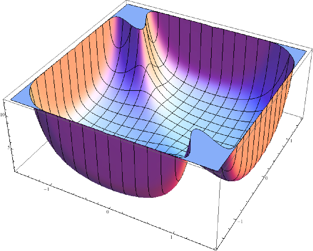
Note that this function (see Figure 1) has singularities on all four sides of the region of integration, with particularly troublesome singularities at $(\pi/2,-\pi/2)$ and $(-\pi/2,\pi/2)$ . However, after making the substitutions $s\leftarrow\pi/2-s,\;t\leftarrow\pi/2-t$ and $r\leftarrow s/t$ , and taking advantage of the symmetry evident from Figure 1, we obtain

	$\displaystyle c_{5,0}$	$\displaystyle=$	$\displaystyle 2\pi\int_{0}^{\pi/2}\int_{0}^{1}\frac{t\,{\bf K}(\cos(rt))\,{\bf K}(\cos t)\,{\rm d}r\,{\rm d}t}{\sqrt{\sin^{2}(rt)\sin^{2}t+4\sin^{2}(t(1+r))}}$		(245)
			$\displaystyle{}+2\pi\int_{0}^{\pi/2}\int_{0}^{1}\frac{t\,{\bf K}(\cos(rt))\,{\bf K}(\cos t)\,{\rm d}r\,{\rm d}t}{\sqrt{\sin^{2}(rt)\sin^{2}t+4\sin^{2}(t(1-r))}}\,,$		(245)

which is significantly better behaved (although these integrands still have singularities on two of the four sides of the region). As a result, we were able to compute $c_{5,0}$ with this formula to 120-digit accuracy, using 240-digit working precision. This run required a parallel computation (using the MPI parallel programming library) of 43.2 minutes on 512 CPUs (1024 cores) of the “Franklin” system at the National Energy Research Scientific Computing Center at the Lawrence Berkeley National Laboratory. The final result matched the value that we had previously calculated using (5) (see [9]) to 120-digit accuracy.

This same strategy was successful for several other 2-D integrals. For example, we computed $c_{6,0}$ to 116-digit accuracy, which again matched the value we had previously computed, in 64.8 minutes on 1024 cores of the Franklin system. In the case of $c_{6,1}$ , the transformation described above for $c_{5,0}$ converted the integrand function of (240) into a completely well-behaved function, without any singularities. As a result, we were able to compute $c_{6,1}$ to 120-digit accuracy using only an Apple Intel-based workstation with four computational cores, in 28 minutes. As before, the result matched the earlier calculation.

As already noted, complex numbers are avoided in integral (228) by writing it as

s_{6,1}=\int_{0}^{\frac{1}{3}}D(y)\int_{0}^{\frac{1}{2}}\frac{4z\,f(A_{-}/A_{+})}{A_{+}\sqrt{1-4z^{2}}}\,{\rm d}z\,{\rm d}y

(246)

where

f(x):=\left\{\begin{array}[]{lll}{\rm arctanh}\left(\sqrt{x}\right)/\sqrt{x}&\mbox{ for }&x>0\\ 1&\mbox{ for }&x=0\\ \arctan\left(\sqrt{-x}\right)/\sqrt{-x}&\mbox{ for }&x<0\end{array}\right.

yields positive real numbers within the rectangle of integration. We were able to confirm that the double integral (246) yields the first 120 of the 1200 decimal places obtained, far more easily, from the single integral (235).

8 Conclusions

Despite some notable progress in discovering and proving new results, we are left with 8 outstanding conjectures.⁶⁶ 6 The conjecture in (112) was later proven by contour integration — see [27]. Of these, 5 have their first instances in Equations (105) to (108) and Equation (112) of Section 5.1, with 3 outliers, in Equations (131), (223) and (231).

Conjecture (105) lies deep in 4-dimensional quantum field theory, but it is reasonable to suppose that it might be derivable from the two-dimensional conjectures (106), (107) and (108), together with their proven sign-changed variants in (109), (110) and (111).

The conjectural integer relations (131) and (136) may be provable by adding rational data such as (132) to a set of recursions richer than those considered in [26, 60].

The real challenge is set by the remarkable sum rule (220), with a dispersive presentation (221), a non-dispersive presentation (222) and a kindergarten analogue (223).

Acknowledgements.

We are most grateful to Andrei Davydychev, for elucidation of dilogarithms obtained in quantum field theory, to Stefano Laporta, for the astute observations in 4-dimensional quantum field theory from which our work arose, to Bas Tausk, for advice on Mellin–Barnes transforms, and to John Zucker, for several pertinent observations regarding integrals of elliptic integrals.

References

[1] M. Abramowitz and I.A. Stegun, Handbook of Mathematical Functions, NBS (now NIST), 1965.
[2] V. Adamchik, “The evaluation of integrals of Bessel functions via G-function identities,” J. Computational and Applied Math, 64 (1995), 283–290.
[3] Gert Almkvist and Bruce Berndt, “Gauss, Landen, Ramanujan, the Arithmetic-Geometric Mean, Ellipses, $\pi$ , and the Ladies Diary,” American Mathematical Monthly, 95 (1988), 585–608.
[4] Kendall E. Atkinson, An Introduction to Numerical Analysis, John Wiley and Sons, New York, 1978.
[5] David H. Bailey, “Integer relation detection,” Computing in Science and Engineering, Jan-Feb, 2000, 24–28.
[6] David H. Bailey and Jonathan M. Borwein, “Highly parallel, high-precision numerical integration,” manuscript, Jun 2006; LBNL-57491, http://crd.lbl.gov/~ dhbailey/dhbpapers/quadparallel.pdf .
[7] D. Bailey, J. Borwein, N. Calkin, R. Girgensohn, R. Luke, and V. Moll, Experimental Mathematics in Action, AK Peters, 2007.
[8] David H. Bailey, Jonathan M. Borwein and Richard E. Crandall, “Integrals of the Ising class,” J. Physics A: Mathematical and General, 39 (2006), 12271–12302, http://crd.lbl.gov/~ dhbailey/dhbpapers/ising.pdf .
[9] David H. Bailey, Jonathan M. Borwein and Richard E. Crandall,“Ising data,” http://crd.lbl.gov/~ dhbailey/dhbpapers/ising-data.pdf .
[10] David H. Bailey, David Borwein, Jonathan M. Borwein and Richard Crandall, “Hypergeometric forms for Ising-class integrals,” Experimental Mathematics, 16 (2007), 257–276, http://crd.lbl.gov/~ dhbailey/dhbpapers/meijer.pdf .
[11] David H. Bailey, Jonathan M. Borwein and Richard E. Crandall, “Box integrals”, Journal of Computational and Applied Mathematics, 206 (2007), 196–208, http://crd.lbl.gov/~ dhbailey/dhbpapers/boxintegrals.pdf .
[12] David H. Bailey and David J. Broadhurst, “Parallel integer relation detection: techniques and applications,” Math. Comp., 70 2001, 1719–1736, http://crd.lbl.gov/~ dhbailey/dhbpapers/ppslq.pdf .
[13] David H. Bailey, Yozo Hida, Xiaoye S. Li and Brandon Thompson, “ARPREC: An Arbitrary Precision Computation Package,” 2002, http://crd.lbl.gov/~ dhbailey/dhbpapers/arprec.pdf . The corresponding software is available at http://crd.lbl.gov/~ dhbailey/mpdist .
[14] David H. Bailey, Xiaoye S. Li and Karthik Jeyabalan, “A comparison of three high-precision quadrature schemes,” Experimental Mathematics, 14 (2005), 317–329, http://crd.lbl.gov/~ dhbailey/dhbpapers/quadrature.pdf .
[15] W. N. Bailey, Generalized Hypergeometric Series, Cambridge University Press, Cambridge, 1935.
[16] W. N. Bailey, “Some infinite integrals involving Bessel functions,” Proc. London Math. Soc., 40 (1936), 37–48.
[17] W. N. Bailey, “Some infinite integrals involving Bessel functions (II),” J. London Math. Soc., 11 (1936), 16–20.
[18] P. Barrucand, “A combinatorial identity,” Problem 75-4, SIAM Rev., 17 (1975), 168.
[19] V. Bârsan, “A two-parameter generalization of the complete elliptic integral of the second kind,” preprint, 2007, http://arxiv.org/PS_cache/arxiv/pdf/0708/0708.2325v1.pdf .
[20] Gabriel Barton, Introduction to dispersion techniques in field theory, Lecture Notes and Supplements in Physics, W.A. Benjamin, New York and Amsterdam, 1965.
[21] T. Blum and Y. Shapir, “Lattice magnetic walks,” J. Phys., A27 (1994), 295–315, http://arxiv.org/PS_cache/cond-mat/pdf/9310/9310024v1.pdf .
[22] Jonathan M. Borwein and David H. Bailey, Mathematics by Experiment: Plausible Reasoning in the 21st Century, AK Peters, Natick, MA, 2004. Second expanded edition, 2008.
[23] Jonathan M. Borwein, David H. Bailey and Roland Girgensohn, Experimentation in Mathematics: Computational Paths to Discovery, AK Peters, Natick, MA, 2004.
[24] Jonathan M. Borwein and Peter B. Borwein, Pi and the AGM: A Study in Analytic Number Theory and Computational Complexity, CMS Monographs and Advanced books in Mathematics, John Wiley, Hoboken, NJ, 1987.
[25] J.M. Borwein, P.B. Borwein and F. Garvan, “Some cubic modular identities of Ramanujan,” Trans. Amer. Math. Soc., 343 (1994), 35–48.
[26] Jonathan Borwein and Bruno Salvy, “A proof of a recursion for Bessel moments,” D-drive Preprint 346, 2007, http://locutus.cs.dal.ca:8088/archive/00000346/ .
[27] David Broadhurst, “Elliptic integral evaluation of a Bessel moment by contour integration of a lattice Green function,” http://arxiv.org/abs/0801.4813 .
[28] D.J. Broadhurst, “The master two-loop diagram with masses”, Zeit. Phys., C47 (1990), 115–124.
[29] D.J. Broadhurst, “Massive three-loop Feynman diagrams reducible to SC* primitives of algebras of the sixth root of unity,” Eur. Phys. J., C8 (1999), 311–333, http://arxiv.org/PS_cache/hep-th/pdf/9803/9803091v1.pdf .
[30] D.J. Broadhurst, J. Fleischer and O.V. Tarasov, “Two-loop two-point functions with masses: Asymptotic expansions and Taylor series, in any dimension,” Zeit. Phys., C60 (1993), 287–302, http://arxiv.org/PS_cache/hep-ph/pdf/9304/9304303v1.pdf .
[31] R.E. Cutkosky, “Some applications of the generalized unitarity relation,” Phys. Rev. Lett., 4 (1960), 624–626; “Singularities and discontinuities of Feynman amplitudes,” J. Math. Phys., 1 (1960), 429–433.
[32] D. Cvetkovic, P. Fowler, P. Rowlinson and D. Stevanovic, “Constructing fullerene graphs from eigenvalues and angles,” Linear Algebra and its Applications, 356 (2002), 37–56.
[33] A.I. Davydychev and R. Delbourgo, “Explicitly symmetrical treatment of three body phase space,” J. Phys., A37 (2004), 4871–4886, http://arxiv.org/PS_cache/hep-th/pdf/0311/0311075v1.pdf .
[34] A.I. Davydychev and J.B. Tausk, “Two-loop self-energy diagrams with different masses and the momentum expansion,” Nucl. Phys., B397 (1993), 123–142, http://www.higgs.de/~ davyd/papers/dt1.pdf .
[35] A.I. Davydychev and J.B. Tausk, “A magic connection between massive and massless diagrams,” Phys. Rev., D53 (1996), 7381–7384, http://arxiv.org/PS_cache/hep-ph/pdf/9504/9504431v1.pdf .
[36] C. Domb, “On the theory of cooperative phenomena in crystals,” Advances in Phys., 9 (1960), 149–361.
[37] A. Erdélyi, W. Magnus, F. Oberhettinger and F.G. Tricomi, Higher Transcendental Functions, Volumes 1–3, McGraw-Hill, 1953.
[38] M.L. Glasser, “Definite integrals of the complete elliptic integral K,” J. Res. NBS, 80B (1976), 313–323.
[39] M.L. Glasser, “A two-parameter generalization of the complete elliptic integral of the second kind,” HAIT Journal of Science and Engineering A, in press, 2007, http://arxiv.org/PS_cache/arxiv/pdf/0709/0709.1289v1.pdf .
[40] S. Groote, “Lectures on configuration space methods for sunrise type diagrams,” International Research Workshop on Calculations for Modern and Future Colliders (CALC 2003), http://arxiv.org/PS_cache/hep-ph/pdf/0307/0307290v1.pdf .
[41] S. Groote, J.G. Korner and A.A. Pivovarov, “On the evaluation of a certain class of Feynman diagrams in x- space: Sunrise-type topologies at any loop order,” Annals Phys., 322 (2007), 2374–2445, http://arxiv.org/PS_cache/hep-ph/pdf/0506/0506286v1.pdf .
[42] A.J. Guttmann and T. Prellberg, “Staircase polygons, elliptic integrals, Heun functions and lattice Green functions,” Phys. Rev., E47 (1993), 2233–2236.
[43] J.A. Hendrickson, Jr., “On the enumeration of rectangular (0,1)-matrices,” Journal of Statistical Computation and Simulation, 51 (1995), 291–313.
[44] R.S. Hijjawi, “Lattice Green’s function for the diamond lattice,” International Journal of Theoretical Physics, 45 (2006), 135–146.
[45] R. Jost, J.M. Luttinger and M. Slotnick, “Distribution of recoil nucleus in pair production by photons,” Phys. Rev., 80 (1950), 189–196.
[46] G.S. Joyce, “Lattice Green function for the anisotropic face centred cubic lattice,” J. Phys., 4 (1971), L53–L56.
[47] G.S. Joyce, “Exact evaluation of the body centred cubic lattice Green function,” J. Phys., 4 (1971), 1510–1512.
[48] G.S. Joyce, “On the simple cubic lattice Green function,” Philosophical Transactions of the Royal Society of London, Mathematical and Physical Sciences, 273 (1973), 583–610.
[49] G.S. Joyce, “On the cubic lattice Green functions,” Philosophical Transactions of the Royal Society of London, Mathematical and Physical Sciences, 445 (1994), 463–477.
[50] G.S. Joyce and I.J. Zucker, “On the evaluation of generalized Watson integrals,” Proceeding of the American Mathematical Society, 133 (2004), 71–81.
[51] G. Källén, Quantum Electrodynamics, Springer-Verlag, 1972.
[52] G. Källén and A. Sabry, “Fourth order vacuum polarization”, Kgl. Danske Videnskab. Selskab. Mat.-Fys. Medd., 29 (1955), #17.
[53] H.A. Kramers, “La diffusion de la lumière par les atomes,” Atti Congresso Internatzionale dei Fisici Como, 2 (1927), 545–557.
[54] R. de L. Kronig, “On the theory of the dispersion of X-rays,” Journal of the Optical Society of America and Review of Scientific Instruments, 12 (1926), 547–557.
[55] S. Laporta, “High precision calculation of multiloop Feynman integrals by difference equations,” Int. J. Mod. Phys., A15 (2000), 5087–5159, http://arxiv.org/PS_cache/hep-ph/pdf/0102/0102033v1.pdf .
[56] S. Laporta, “High precision epsilon expansions of massive four loop vacuum bubbles,” Phys. Lett., B549 (2002), 115–122, http://arxiv.org/PS_cache/hep-ph/pdf/0210/0210336v1.pdf .
[57] L. Lewin Polylogarithms and Associated Functions, North Holland, 1981.
[58] I. Mannari and C. Kawabata, “Extend Watson integrals and their derivatives,” Res. Notes No 15, Dept. of Physics, Okayama University, Okayama, Japan, 1964.
[59] F. Oberhettinger, Tables of Fourier Transforms and Fourier Transforms of Distributions, Springer-Verlag, New York, 1990.
[60] Stéphane Ouvry, “Random Aharonov-Bohm vortices and some exactly solvable families of integrals,” Journal of Statistical Mechanics: Theory and Experiment, 1 (2005), P09004, http://arxiv.org/abs/cond-mat/0502366 .
[61] C.G. Papadopoulos and M. Worek, “Multi-parton cross sections at hadron colliders,” Eur. Phys. J., C50 (2007), 843–856, http://arxiv.org/PS_cache/hep-ph/pdf/0512/0512150v2.pdf .
[62] Marko Petkovsek, Herbert S. Wilf and Doron Zeilberger, A = B, AK Peters, Natick, MA, 1996.
[63] A.P. Prudnikov, Yu.A. Brychkov and O.I. Marichev, Integrals and Series, Volumes 1–3, Taylor and Francis, London, 1986.
[64] A. Ronveaux (Ed.), Heun’s Differential Equations, The Clarendon Press, 1995.
[65] A. Sabry, “Fourth order spectral functions for the electron propagator”, Nucl. Phys., 33 (1962), 401–430.
[66] N.J.A. Sloane and S. Plouffé, The Encyclopedia of Integer Sequences, Academic Press, San Diego, 1995, ISBN: 0-12-558630-2.
[67] H. Takahasi and M. Mori, “Double exponential formulas for numerical integration,” Publications of RIMS, Kyoto University, 9 (1974), 721–741.
[68] F.G. Tricomi, Bollettino Unione Matematica Italiana, 14 (1935), 213–218; 277–282; 15 (1936), 102–195.
[69] N.G. van Kampen, “S-Matrix and causality condition. I. Maxwell field”, Phys. Rev., 89 (1953), 1072–1079; “II. Nonrelativistic particles”, 91 (1953), 1267–1276.
[70] Yung-Li Wang, Chris Wentworth and B. Westwanski, “Linked-cluster expansion for quantum spin systems and the perpendicular susceptibility of the Ising model,” Phys. Rev., B32 (1985), 1805–1812.
[71] G.N. Watson, “Three triple integrals,” Q. J. Math. (Oxford), 10 (1939), 266–276.
[72] G.N. Watson, A Treatise on the Theory of Bessel Functions, second edition, Cambridge University Press, 1944.

Elliptic integral evaluations of Bessel moments

Abstract

1 Introduction

2 Two Bessel functions

3 Three Bessel functions

Nomenclature.

3.1 The odd moments s3,2​k+1s_{3,2k+1}

3.2 The odd moments c3,2​k+1c_{3,2k+1}

3.3 The even moments c3,2​kc_{3,2k}

Remark.

3.4 Continued fraction

3.5 Double integrals

3.6 Hypergeometric series

3.7 Integrals of elliptic integrals

3.8 Sum rule

4 Four Bessel functions

4.1 The odd moments s4,2​k+1s_{4,2k+1}

4.2 Dispersion relation

4.3 The odd moments c4,2​k+1c_{4,2k+1}

4.4 The even moment c4,0c_{4,0}

4.5 Sum rule

4.6 The even moment c4,2c_{4,2}

4.7 Further evaluation of integrals

4.8 Further evaluations of sums

4.9 Relation to Meijer’s G-function

4.10 Another continued fraction

4.11 The even moment s4,0s_{4,0}

4.12 Tabular summary

5 Five Bessel functions

5.1 Conjectural evaluations of Feynman diagrams

Notation.

5.2 The odd moments t5,2​k+1t_{5,2k+1}

5.3 Double integrals

5.4 Single integrals from polar coordinates

5.5 Single integrals over discontinuities

5.6 Relations between elliptic integrals

5.7 Expansions near singularities

5.8 A modular identity from quantum field theory

5.9 A discrete sum rule

5.10 Sum rules for diamond and cubic lattice integers

5.11 Cubic modular equations

5.12 Integral sum rules

5.13 The even moment c5,0c_{5,0}

6 Six Bessel functions

6.1 The odd moments t6,2​k+1t_{6,2k+1}

6.2 The odd moments s6,2​k+1s_{6,2k+1}

6.3 Sum rules

6.4 The odd moments c6,2​k+1c_{6,2k+1}

6.5 The even moment c6,0c_{6,0}

7 Computational notes

7.1 Multi-dimensional quadrature

8 Conclusions

Acknowledgements.

References

3.1 The odd moments $s_{3,2k+1}$

3.2 The odd moments $c_{3,2k+1}$

3.3 The even moments $c_{3,2k}$

4.1 The odd moments $s_{4,2k+1}$

4.3 The odd moments $c_{4,2k+1}$

4.4 The even moment $c_{4,0}$

4.6 The even moment $c_{4,2}$

4.11 The even moment $s_{4,0}$

5.2 The odd moments $t_{5,2k+1}$

5.13 The even moment $c_{5,0}$

6.1 The odd moments $t_{6,2k+1}$

6.2 The odd moments $s_{6,2k+1}$

6.4 The odd moments $c_{6,2k+1}$

6.5 The even moment $c_{6,0}$