The rotation curves of flattened Sérsic bulges
Abstract
I present a method to deproject the observed intensity profile of an axisymmetric bulge with arbitrary flattening to derive the 3D luminosity density profile and to calculate the contribution of the bulge to the rotation curve. I show the rotation curves for a family of fiducial bulges with Sérsic surface brightness profiles and with various concentrations and intrinsic axis ratios. Both parameters have a profound impact on the shape of the rotation curve. In particular, I show how the peak rotation velocity, as well as the radius where it is reached, depend on both parameters.
I also discuss the implications of the flattening of a bulge for the decomposition of a rotation curve and use the case of NGC 5533 to show the errors that result from neglecting it. For NGC 5533, neglecting the flattening of the bulge leads to an overestimate of its mass-to-light ratio by approximately 30% and an underestimate of the contributions from the stellar disc and dark matter halo in the regions outside the bulge-dominated area.
Keywords:
galaxies: bulges – galaxies: kinematics and dynamics – galaxies: structure1 Introduction
Rotation curves of spiral galaxies are one of the prime methods to probe the mass distribution on galactic scales. The discovery, made in the 1970s (Rogstad & Shostak, 1972; Roberts & Whitehurst, 1975; Bosma, 1978; Bosma, 1981), that rotation curves remain flat till the last measured points, well outside the optical discs, provided the decisive evidence for the presence of large amounts of dark matter in galaxies. Unfortunately, however, it has proven difficult to gain detailed knowledge about the distribution of dark matter in galaxies. This is primarily due to the fact that, with the exception of the lowest surface brightness galaxies, the stars in galaxies contribute a significant, but not precisely known, fraction to the overall gravitational potential (Persic et al., 1996; de Blok & McGaugh, 1997; Palunas & Williams, 2000; Noordermeer, 2006).
To determine the contribution from the stars to an observed rotation curve, the full 3D structure of the stellar mass distribution needs to be known. In most disc galaxies, the bulk of the stars can be divided between a flat disc and a thicker central bulge. Once an accurate bulge-disc decomposition has been performed, it is relatively straightforward to calculate the contribution to the rotation curve from the disc, given its simple, effectively 2D structure (Casertano, 1983, e.g.). For the central bulge, however, the situation is more complex. Historically, it was often assumed that bulges follow an luminosity-profile (de Vaucouleurs, 1958; van Houten, 1961; de Vaucouleurs, 1974). For dynamical purposes, they were often further assumed to be spherically symmetric bodies, in which case the observed intensity profile can be deprojected and the gravitational potential calculated easily (Young, 1976, e.g.). In reality, however, bulges are generally neither spherical, nor do they follow the density-profile (Andredakis & Sanders, 1994; Andredakis et al., 1995; Erwin & Sparke, 1999; Graham, 2001; Erwin & Sparke, 2002; Noordermeer & van der Hulst, 2007).
Several papers have addressed various aspects related to the properties of non-spherical bulges with a more general luminosity density profile. The problem of deprojecting a non-spherical bulge was already addressed by Stark (1977). The dynamical properties of spherical bodies following a general luminosity profile have been studied by Ciotti (1991). This analysis was extended by Trujillo et al. (2002), who studied triaxial systems following the luminosity law and presented an analytical expression to approximate the deprojected, 3D luminosity density profile.
For the purpose of rotation curve analysis, one usually assumes axisymmetry for all components in the galaxy and ignores the triaxial nature of the bulge. Most bulges are only mildly triaxial (Bertola et al., 1991; Méndez-Abreu et al., 2007), so that the errors stemming from this assumption are generally small. Accounting for the full triaxiality of the bulges merely complicates the calculations in this context. In fact, given the fact that rotation curves are by definition one-dimensional quantities, they are intrinsically unsuitable to account for deviations from axisymmetry. A proper treatment of the dynamical effects of triaxial bulges requires two- or three-dimensional modelling of the gas flows in their potentials. The flattening of the bulge in the vertical direction, on the other hand, is often significant (Bertola et al., 1991; Noordermeer & van der Hulst, 2007, e.g.). It is also dynamically important and should not be neglected, even in the axisymmetric approximation.
In this paper, I study the 3D luminosity density of axisymmetric bulges with various intrinsic flattenings and their contribution to the rotation curve of a galaxy. In section 2, I present the relevant equations to deproject the observed surface brightness profile of a bulge to the 3D luminosity density and to calculate its contribution to the rotation curve. Although some of the equations in section 2 can be applied to an arbitrary bulge surface brightness profile, I specifically focus on bulges with a Sérsic luminosity profile (Sérsic, 1968). In section 3, I present the bulge rotation curves for a range of parameters and discuss various properties of the curves. I show the effects of the concentration and flattening of the bulge on the shape of its rotation curve and in particular on the location and height of the peak. Finally, in section 4, I briefly discuss the implications of the results from the preceding sections. In particular, I use the example of the Sab galaxy NGC 5533 to illustrate the errors which result from neglecting the flattening of the bulge when decomposing a rotation curve.
2 Derivation of the rotation curves
2.1 Deprojection of the observed surface density distribution
The first step in our calculations involves the deprojection of the observed surface density distribution, to yield the 3D luminosity density. This has been done for the general triaxial situation by Stark (1977). Here, I consider the simpler configuration of an axisymmetric spheroid, symmetric with respect to the plane of the galactic disc.
Let us define an -coordinate system such that the -plane coincides with the plane of symmetry of the galaxy. The luminosity density can then be written as , with and the intrinsic axis ratio of the bulge isodensity surfaces.

A second coordinate system, , can be defined corresponding to the observational configuration. lies along the line of sight and is inclined by an angle with respect to the -axis. The -axis coincides with the -axis; both are defined to lie along the line of nodes. is the axis that is perpendicular to on the plane of the sky; in practice this means that lies along the minor axis of the galaxy. See figure 1 for an overview of the coordinate systems. The and coordinate systems are related by the following transformation matrices:
| (1) |
| (2) |
With these coordinates, the projected intensity at each position on the sky can be written, in the case of an optically thin medium, as
| (3) |
It can be shown that the projected intensity distribution on the sky has an ellipsoidal shape, where the ellipticity of the projected image is related to the intrinsic axis ratio and the inclination angle as
| (4) |
Thus, the problem is reduced to finding the relation between the projected intensity at the line of nodes () and the density . Once the intensity at the line of nodes is derived, the rest of the image can be reconstructed using equation 4.
Given a position at the line of nodes (), the relation between and is (see equations 1, 2):
| (5) | |||||
| (6) | |||||
| (7) |
Then, setting in equation 3, changing the integration variable from to and using equation 7, the projected intensity at the line of nodes becomes:
This is an Abel-integral, which can be inverted (e.g. Binney & Tremaine, 1987, app. 1.B4) to obtain the following equation, which gives the 3D luminosity density distribution when the observed major-axis intensity profile is given:
| (9) |


2.2 Calculation of the rotation curve
Now, assuming that the observed emission traces mass and that the mass-to-light ratio is constant throughout the bulge, equation 9 also gives the 3D mass density distribution in the bulge (except for a constant factor for the actual value of the mass-to-light ratio, ). The derivation of the corresponding rotation curve is then straightforward and is described in Binney & Tremaine (1987). Inserting equation 9 into their equation 2-91, we get for the rotation curve:
where is the eccentricity of the bulge: .
This equation is valid for any given observed intensity profile ; no prior assumptions have been made regarding the shape of the light or density profiles, except that of spheroidal symmetry. In principle, one could directly derive the rotation curve for any given intensity profile by numerically calculating the derivative and evaluating the integral. In practice, the intensity profiles of many bulges follow a general Sérsic profile (Sérsic, 1968), defined as:
| (11) |
Here, is the central surface brightness and is a concentration parameter that describes the curvature of the profile in a radius-magnitude plot. For , equation 11 reduces to the well-known de Vaucouleurs profile (de Vaucouleurs, 1948), whereas describes a simple exponential profile. is the characteristic radius, which is related to the effective radius (, the radius which encompasses 50% of the light) as . is a scaling constant that is defined such that it satisfies , with and the incomplete and complete gamma functions respectively. Given a Sérsic bulge, one can evaluate the derivative analytically:
| (12) |
Inserting this into equation 2.2, we get the following, final equation for the bulge rotation curve:
| (14) |
3 Properties of the rotation curves
Equation 14 can, to my knowledge, generally not be solved analytically. Instead, it was evaluated numerically, using algorithms from Press et al. (1992)11 1 A FORTRAN program to evaluate the integrals in equation 14 is available upon request from the author., for various parameter combinations.
Of particular interest are the effects of the flattening, , and the concentration, , of the bulges on the resulting rotation curves. In figure 3, I show the rotation curves for a family of fiducial bulges with various concentrations and axis ratios, but with and scaled such that all bulges have equal total luminosity () and effective radius (). For simplicity, I assumed a mass-to-light ratio of . The range of values for and which I consider here spans the observed values in bulges of nearby spiral galaxies of various morphological types (Andredakis et al., 1995; Khosroshahi et al., 2000; Graham, 2001; Noordermeer & van der Hulst, 2007), although I also include a number of prolate bulges with which are not observed in reality. Note that observed bulges show a general trend of increasing luminosity and radius with increasing . For easy comparison, however, I choose to study bulges with equal luminosity and effective radii here; the rotation curves shown in figure 3 can be scaled easily for bulges with different mass or radius.
It is clear that both the flattening and the concentration of the bulge have a large influence on the shape of the rotation curves. Varying either parameter changes both the radius where the rotation curve peaks and the corresponding peak velocity. This is illustrated in a quantitative way in figure 3. As expected, a flattened bulge has a higher peak rotational velocity than a spherical one. Interestingly, the strength of the correlation is a weak function of the concentration, being largest for less concentrated bulges. For , a highly flattened bulge with an intrinsic axis ratio of has a peak velocity about 22% higher than the spherical case. For a highly concentrated bulge (), the difference is approximately 17%.
Not surprising either, more centrally concentrated bulges reach the peak in their rotation curve at smaller radii. Cored bulges with reach the maximum rotation velocity between 1.5 and 2.0 effective radii, depending on . Concentrated bulges with , on the other hand, peak at very small radii, within 2% of the effective radius, with the exact radius again depending on .
The dependence of the location of the peak in the rotation curve on the flattening of the bulge is somewhat less expected. The bottom left hand panel in figure 3 shows that the peak is reached at smaller radii in more flattened bulges. The strength of the correlation depends on the concentration of the bulge: for , a highly flattened bulge with an intrinsic axis ratio of reaches the peak rotation velocity at a 12% smaller radius than the spherical case, whereas for , this difference is 18%. As an aside, I note that a spherical bulge () with a Sérsic parameter of reaches the peak rotational velocity at exactly one effective radius.
Finally, for a given total mass, effective radius and intrinsic axis ratio, the peak rotational velocity is lowest for a bulge with , with both more and less concentrated bulges having higher peak rotation velocities.
4 Discussion
It is now common knowledge that morphologically, the assumptions that bulges are spherical and have an luminosity-profile are poor descriptions of reality. Our analysis shows that this is also true dynamically. As figures 3 and 3 illustrate, the flattening and concentration of a bulge have a strong influence on the shape of its rotation curve. Specifically, non-spherical bulges and bulges with a concentration parameter different from 4 have rotation curves with very different peak velocities and radii than a ‘classical’ spherical de Vaucouleurs bulge.
The dependence of the peak velocity on the flattening of the bulge has important consequences in the decomposition of an observed rotation curve into contributions from the various components in a galaxy. In practice, the bulge contribution in such a decomposition is often determined by scaling up the bulge mass-to-light ratio until the peak of the bulge rotation curve matches the amplitude of the observed curve at that radius. If we neglect the intrinsic flattening of a bulge and instead derive its rotation curve under the assumption that it is spherically symmetric, we will underestimate the peak velocity (see figure 3). As a result, we will need to assume a higher mass-to-light ratio in order to explain the observed rotation velocity at the peak radius. Figure 3 shows that the difference in peak velocity between a spherical bulge and a highly flattened bulge with is of the order of 20%. Since the mass-to-light ratio is proportional to the square of the bulge rotation velocity (equation 14), the error in the former would be more than 40%.
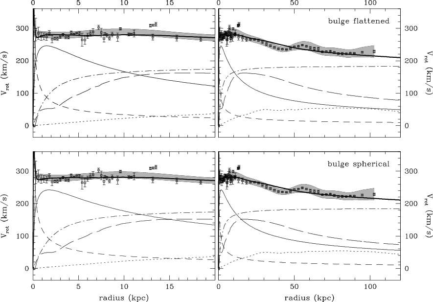
To illustrate this effect, I show in figure 4 the rotation curve decomposition for the massive Sab galaxy NGC 5533. Its rotation curve was measured from a combination of optical spectroscopic data and Hi observations by Noordermeer et al. (2007). R-band photometry for this galaxy was presented by Noordermeer & van der Hulst (2007), as well as a detailed study of the properties of its bulge and disc. The effects of the seeing on the measured bulge parameters were corrected for, using the deconvolutions from Graham (2001). The bulge was found to be highly flattened, , making this galaxy an interesting test-case for the effect described above.
Based on the derived properties of the bulge from Noordermeer & van der Hulst (2007), I have derived two versions of its contribution to the rotation curve: one accounting correctly for its flattening using equation 14 and another by neglecting the flattening and assuming . The contribution of the stellar and gaseous discs were calculated using the prescriptions from Casertano (1983), assuming a vertical scale height of one fifth of the stellar disc scale length. For simplicity, the dark matter halo was assumed to have an isothermal density profile. Finally, in order to explain the rapid rise of the rotation curve in the centre, a central black hole was added to the model. The contributions from the various components were then added and the 5 free model parameters (the R-band mass-to-light ratios and for the bulge and disc respectively, the core radius and central density of the dark halo and the mass of the black hole ) were adapted in a simple minimisation procedure to obtain the best fitting model rotation curve. The values for the fitted parameters are listed in table 1.
| () | 2.8 | 0.1 | 3.7 | 0.1 |
| () | 5.0 | 0.2 | 4.4 | 0.2 |
| () | 1.4 | 0.2 | 1.7 | 0.2 |
| () | 0.31 | 0.08 | 0.23 | 0.05 |
| () | 2.7 | 0.6 | 3.4 | 0.6 |
Figure 4 shows that equally good fits can be made with both bulge rotation curves; neglecting the bulge flattening does not have a noticeable effect on the quality of the model in this case. However, it is clear from table 1 that, when the bulge is assumed to be spherically symmetric, a higher mass-to-light ratio has to be assumed to explain the observed rotation velocities around the peak radius of 2 kpc. In this case, the difference between the two values for is 32%.
Figure 4 and table 1 also illustrate a more subtle effect. The effect of the flattening of the bulge on its rotation curve contribution diminishes rapidly with radius (see also figure 3). Outside about 5 effective radii, the flattening has virtually no effect anymore on the amplitude of the bulge rotation curve, which then only depends on the total mass of the bulge. Thus, because we were forced to assume a higher mass-to-light ratio for the spherical bulge, its contribution at large radii is larger than in the flattened case. As a result, the derived contribution of the disc is somewhat smaller and the dark matter halo is less concentrated, with a 21% larger core radius. The same effect occurs when we assume an NFW density profile (Navarro et al., 1997) for the dark matter halo. In that case, we find again that the concentration of the halo is significantly smaller (by about 15%) when we assume that the bulge is spherical, compared to the model where we account for the flattening of the bulge.
In conclusion, the results shown in this paper prove that, for a detailed study of the dynamical structure of disc galaxies with a sizeable bulge, it is crucial to properly account for the concentration and intrinsic flattening of the latter.
Acknowledgements
I would like to thank Mike Merrifield for stimulating discussions and helpful suggestions during the preparations of this paper. I am also grateful to the referee, Enrico Corsini, for useful suggestions.
References
- Andredakis et al. (1995) Andredakis Y. C., Peletier R. F., Balcells M., 1995, MNRAS, 275, 874
- Andredakis & Sanders (1994) Andredakis Y. C., Sanders R. H., 1994, MNRAS, 267, 283
- Bertola et al. (1991) Bertola F., Vietri M., Zeilinger W. W., 1991, ApJ, 374, L13
- Binney & Tremaine (1987) Binney J., Tremaine S., 1987, Galactic dynamics. Princeton, NJ, Princeton University Press, 1987
- Bosma (1978) Bosma A., 1978, PhD thesis, Rijksuniversiteit Groningen
- Bosma (1981) Bosma A., 1981, AJ, 86, 1825
- Casertano (1983) Casertano S., 1983, MNRAS, 203, 735
- Ciotti (1991) Ciotti L., 1991, A&A, 249, 99
- de Blok & McGaugh (1997) de Blok W. J. G., McGaugh S. S., 1997, MNRAS, 290, 533
- de Vaucouleurs (1948) de Vaucouleurs G., 1948, Annales d’Astrophysique, 11, 247
- de Vaucouleurs (1958) de Vaucouleurs G., 1958, ApJ, 128, 465
- de Vaucouleurs (1974) de Vaucouleurs G., 1974, in Shakeshaft J. R., ed., The Formation and Dynamics of Galaxies Vol. 58 of IAU Symposium, Structure, dynamics and statistical properties of galaxies. pp 1–52
- Erwin & Sparke (1999) Erwin P., Sparke L. S., 1999, ApJ, 521, L37
- Erwin & Sparke (2002) Erwin P., Sparke L. S., 2002, AJ, 124, 65
- Graham (2001) Graham A. W., 2001, AJ, 121, 820
- Khosroshahi et al. (2000) Khosroshahi H. G., Wadadekar Y., Kembhavi A., 2000, ApJ, 533, 162
- Méndez-Abreu et al. (2007) Méndez-Abreu J., Aguerri J. A. L., Corsini E. M., Simonneau E., 2007, ArXiv e-prints: 0710.5466, 710
- Navarro et al. (1997) Navarro J. F., Frenk C. S., White S. D. M., 1997, ApJ, 490, 493
- Noordermeer (2006) Noordermeer E., 2006, Ph.D. Thesis, Rijksuniversiteit Groningen
- Noordermeer & van der Hulst (2007) Noordermeer E., van der Hulst J. M., 2007, MNRAS, 376, 1480
- Noordermeer et al. (2007) Noordermeer E., van der Hulst J. M., Sancisi R., Swaters R. S., van Albada T. S., 2007, MNRAS, 376, 1513
- Palunas & Williams (2000) Palunas P., Williams T. B., 2000, AJ, 120, 2884
- Persic et al. (1996) Persic M., Salucci P., Stel F., 1996, MNRAS, 281, 27
- Press et al. (1992) Press W. H., Teukolsky S. A., Vetterling W. T., Flannery B. P., 1992, Numerical recipes in FORTRAN. The art of scientific computing. Cambridge University Press
- Roberts & Whitehurst (1975) Roberts M. S., Whitehurst R. N., 1975, ApJ, 201, 327
- Rogstad & Shostak (1972) Rogstad D. H., Shostak G. S., 1972, ApJ, 176, 315
- Sérsic (1968) Sérsic J. L., 1968, Atlas de Galaxias Australes. Cordoba, Argentina: Observatorio Astronomico, 1968
- Stark (1977) Stark A. A., 1977, ApJ, 213, 368
- Trujillo et al. (2002) Trujillo I., Asensio Ramos A., Rubiño-Martín J. A., Graham A. W., Aguerri J. A. L., Cepa J., Gutiérrez C. M., 2002, MNRAS, 333, 510
- van Houten (1961) van Houten C. J., 1961, Bull. Astron. Inst. Netherlands, 16, 1
- Young (1976) Young P. J., 1976, AJ, 81, 807