Counting Statistics of Non-Markovian Quantum Stochastic Processes

Full counting statistics (FCS) has recently attracted intensive theoretical [1] and experimental [2] attention. The interest stems from the usefulness of FCS as a sensitive diagnostic tool of stochastic electron transport through mesoscopic systems. Detectable mechanisms include quantum-mechanical coherence, entanglement, disorder, and dissipation [1]. Mathematically, FCS encodes the complete knowledge of the probability distribution $P(n,t)$ of the transmitted number $n$ of electrons or, equivalently, of all corresponding cumulants. Non-zero higher order cumulants describe non-Gaussian behavior. The study of counting statistics for stochastic processes in general is of broad relevance for a wide class of problems, also outside mesoscopic physics. For example, rare events, whose study has become an important topic within non-equilibrium statistics of stochastic systems in physics, chemistry, and biology [3], are reflected in higher order cumulants. Efficient methods for evaluating the counting statistics of stochastic processes are therefore of urgent need.

In this Letter, we present a method which unifies and extends a number of earlier approaches to FCS within a generalized master equation (GME) formulation [4, 5, 6]. The earlier approaches have in practice been limited to systems with only a few states [4, 6], or only the first few current cumulants [5]. In contrast, our theory enables studies of a much larger class of problems: Evaluation of zero-frequency current cumulants of very high orders for non-Markovian systems with many states is now possible. Furthermore, the method allows us to develop a general approach to the finite-frequency current noise of non-Markovian transport processes. In the case of finite-frequency noise, we show that not only the memory kernel but also initial system-environment correlations are crucial. Such correlations can be, and have been [6, 7], neglected for non-Markovian processes at low frequencies, but must be included at frequencies comparable with the internal frequencies of the system. We demonstrate our methods on a system of recent experimental relevance, namely transport through a dissipative double quantum dot [7, 8], but they may easily be applied to other electronic (or photonic) counting systems, as well as other counted quantities, such as heat or work, in non-equilibrium systems [9].

Non-Markovian GME. Consider a nanoscale transport system governed by a generic non-Markovian GME of the form [10, 11]

Here, the reduced density matrix of the system $\hat{\rho}(t)$ has been resolved into components $\hat{\rho}(n,t)$ corresponding to the number of electrons $n$ passing through the nanosystem within time-span $[0,t]$. The memory kernel $\mathcal{W}$ describes the influence of the environment on the dynamics of the system, while the inhomogeneity $\hat{\gamma}$ accounts for initial correlations between system and environment. Both $\mathcal{W}$ and $\hat{\gamma}$ decay with time, usually on a comparable timescale, so that $\hat{\gamma}$ is irrelevant for the long-time limit. The inhomogeneity $\hat{\gamma}$ does, however, play a crucial role at finite times. The probability distribution for the number of transferred charges is $P(n,t)=\mathrm{Tr}\{\hat{\rho}(n,t)\}$. The corresponding cumulant generating function (CGF) $\mathcal{S}(\chi,t)$ is defined as $e^{\mathcal{S}(\chi,t)}\equiv\sum_{n}P(n,t)e^{in\chi}$. In Laplace space Eq. (1) leads to the algebraic expression $\hat{\rho}(\chi,z)=\mathcal{G}(\chi,z)[\hat{\rho}(\chi,t=0)+\hat{\gamma}(\chi,z)]$, where $\mathcal{G}(\chi,z)\equiv[z-\mathcal{W}(\chi,z)]^{-1}$ is the resolvent of the kernel, and $\hat{\rho}(\chi,z)\equiv\sum_{n}\int_{0}^{\infty}dt\hat{\rho}(n,t)e^{in\chi-zt}$ and similarly for $\hat{\gamma}(\chi,z)$ and $\mathcal{W}(\chi,z)$. Inverting the Laplace transformation, the CGF then becomes

where $a$ is a real number, chosen such that all singularities of the integrand are situated to the left of the vertical line of integration. We have moreover introduced the notation $\langle\mathcal{G}(\chi,z)\rangle\equiv\mathrm{Tr}\{\mathcal{G}(\chi,z)[\hat{\rho}(\chi,t=0)+\hat{\gamma}(\chi,z)]\}$. Equation (2) contains the full statistical information about the charge transfer process. It is a powerful formal result, but it also leads to useful practical schemes, as we shall now demonstrate.

Zero-frequency FCS. Consider first the zero-frequency cumulants of the current, defined as $\langle\!\langle I^{m}\rangle\!\rangle=\frac{d}{dt}\frac{\partial^{m}\mathcal{S}(\chi,t)}{\partial{(i\chi)^{m}}}|_{\chi\rightarrow 0,t\rightarrow\infty}$, $m=1,2,\ldots$. We assume that the system with the counting field $\chi$ set to zero tends exponentially to a unique stationary state determined by the $1/z$ pole of the resolvent $\mathcal{G}(\chi=0,z)$. The stationary state is given by the eigenvector corresponding to the zero-eigenvalue of $\mathcal{W}\equiv\mathcal{W}(\chi=0,z=0)$, i.e., $\lim_{t\rightarrow\infty}\hat{\rho}(t)=\hat{\rho}^{\rm stat}$, where $\hat{\rho}^{\rm stat}$ is the normalized solution to $\mathcal{W}\hat{\rho}^{\rm stat}=0$. With finite values of $\chi$, an eigenvalue $\lambda_{0}(\chi,z)$ develops adiabatically from the zero-eigenvalue, such that $\lambda_{0}(0,z)=0$, and the long-time behavior is determined by the isolated pole structure $1/[z-\lambda_{0}(\chi,z)]$ of $\mathcal{G}(\chi,z)$ close to zero. This pole $z_{0}(\chi)$ solves

and goes to zero with $\chi$ going to zero, i.e., $z_{0}(0)=0$. We thus find $e^{\mathcal{S}(\chi,t)}\rightarrow\mathcal{D}(\chi)e^{z_{0}(\chi)t}$ for large $t$, where $\mathcal{D}(\chi)$ is a time-independent function depending on the initial conditions and correlations. The current cumulants then read $\langle\!\langle I^{m}\rangle\!\rangle=\frac{\partial^{m}z_{0}(\chi)}{\partial{(i\chi)^{m}}}|_{\chi\rightarrow 0}$. In the Markovian limit for the kernel $\mathcal{W}(\chi,z\rightarrow 0)$ we get $z_{0}(\chi)=\lambda_{0}(\chi,0)$ as found in Refs. [4, 5].

Recursive scheme. When the involved matrices are large, it may be non-trivial to determine the full $\chi$ and $z$ dependence of the eigenvalue $\lambda_{0}(\chi,z)$, and thereafter solve Eq. (3). Instead, we expand the eigenvalue as $\lambda_{0}(\chi,z)=\sum_{k,l=0}^{\infty}\frac{(i\chi)^{k}}{k!}\frac{z^{l}}{l!}c^{(k,l)}$ with $c^{(0,L)}=0$, and calculate the expansion coefficients recursively using Rayleigh-Schrödinger perturbation theory [12]:

with $K,L=0,1,2,\ldots$. Here, $\langle\!\langle\tilde{0}|$ solves $\langle\!\langle\tilde{0}|\mathcal{W}=0$, while $|0^{(0,0)}\rangle\!\rangle$ is the stationary state $\hat{\rho}^{\rm stat}$. Moreover, $\mathcal{\overline{W}}(\chi,z)\equiv\mathcal{W}(\chi,z)-\mathcal{W}$ has been expanded as $\mathcal{\overline{W}}(\chi,z)=\sum_{k,l=0}^{\infty}\frac{(i\chi)^{k}}{k!}\frac{z^{l}}{l!}\mathcal{\overline{W}}^{(k,l)}$ with $\mathcal{\overline{W}}^{(0,0)}=0$. Finally, the pseudoinverse of the kernel is $\mathcal{R}\equiv\mathcal{Q}\mathcal{W}^{-1}\mathcal{Q}$ with $\mathcal{Q}\equiv 1-|0^{(0,0)}\rangle\!\rangle\!\langle\!\langle\tilde{0}|$ ¹¹ 1 Details of the notation can be found in Ref. [13].. With the $c^{(K,L)}$’s at hand we can solve Eq. (3) for $z_{0}(\chi)$ to a given order in $\chi$, and from the expansion $z_{0}(\chi)=\sum_{n=1}^{\infty}\frac{(i\chi)^{n}}{n!}\langle\!\langle I^{n}\rangle\!\rangle$ extract the zero-frequency cumulants of the current:

with $L=0,1,2,\ldots$, and $K,N=1,2,3,\ldots$. For the auxiliary quantity $P^{(K,L)}$, we have $P^{(K,0)}=\delta_{K,0}$, $P^{(0,L)}=\delta_{0,L}$, and $P^{(K,-1)}\equiv 0$.

We illuminate the recursive scheme by evaluating the first three cumulants of the current using Eq. (5); the mean current, the variance (the noise), and the skewness:

Higher order cumulants can be obtained in a similar manner, analytically or numerically. Coefficients of the form $c^{(L,0)}$ are purely Markovian quantities, and the mean current is thus not sensitive to non-Markovian effects, whereas higher order cumulants are [6, 14]. From Eq. (4) we find for the coefficients $c^{(K,L)}$, e.g., $c^{(1,0)}=\langle\!\langle\tilde{0}|\mathcal{\overline{W}}^{(1,0)}|0^{(0,0)}\rangle\!\rangle$, $c^{(1,1)}=\langle\!\langle\tilde{0}|(\mathcal{\overline{W}}^{(1,1)}-\mathcal{\overline{W}}^{(1,0)}\mathcal{R}\mathcal{\overline{W}}^{(0,1)})|0^{(0,0)}\rangle\!\rangle$, and $c^{(2,0)}=\langle\!\langle\tilde{0}|(\mathcal{\overline{W}}^{(2,0)}-2\mathcal{\overline{W}}^{(1,0)}\mathcal{R}\mathcal{\overline{W}}^{(1,0)})|0^{(0,0)}\rangle\!\rangle$. Evaluation of the pseudoinverse $\mathcal{R}$ amounts to solving matrix equations which is feasible even with very large matrices [13]. Numerically, the recursive scheme is stable for very high orders of cumulants ($>20$) as we have tested on simple models.

Double quantum dot. We illustrate our method by considering a model of charge transport through a Coulomb blockaded double quantum dot in a dissipative environment [7]. Maximally one additional electron is allowed on the double quantum dot. The Hamiltonian of the double quantum dot is $\hat{H}_{S}=\frac{\varepsilon}{2}\hat{s}_{z}+T_{c}\hat{s}_{x}$, where the pseudo-spin operators are $\hat{s}_{z}\equiv|L\rangle\!\langle L|-|R\rangle\!\langle R|$ and $\hat{s}_{x}\equiv|L\rangle\!\langle R|+|R\rangle\!\langle L|$, respectively. The tunnel coupling between the two quantums dot levels $|L\rangle$ and $|R\rangle$ is $T_{c}$, while $\varepsilon$ is their detuning. The pseudo-spin system is tunnel-coupled to left ($L$) and right ($R$) leads via the tunnel-Hamiltonian $\hat{H}_{T}=\sum_{k_{\alpha},\alpha=L,R}(V_{k_{\alpha}}\hat{c}^{\dagger}_{k_{\alpha}}|0\rangle\!\langle\alpha|+\mathrm{h.c.})$, with both leads described as non-interacting fermions, i.e., $\hat{H}_{\alpha}=\sum_{k_{\alpha}}\varepsilon_{k_{\alpha}}\hat{c}^{\dagger}_{k_{\alpha}}\hat{c}_{k_{\alpha}},\alpha=L,R$. Dissipation is provided by a reservoir of non-interacting bosons that couple to the $\hat{s}_{z}$ component of the pseudo-spin. The Hamiltonian is then $\hat{H}=\hat{H}_{S}+\hat{H}_{T}+\hat{H}_{L}+\hat{H}_{R}+\hat{H}_{B}+\hat{V}_{B}\hat{s}_{z}$, where $\hat{H}_{B}=\sum_{j}\hbar\omega_{j}\hat{a}_{j}^{\dagger}\hat{a}_{j}$ and $\hat{V}_{B}=\sum_{j}\frac{g_{j}}{2}(\hat{a}_{j}^{\dagger}+\hat{a}_{j})$.

To describe charge transport through the system we trace out the leads following Gurvitz and Prager [15], leading to an equation of motion for the reduced density matrix $\hat{\sigma}=(\hat{\sigma}_{00},\hat{\sigma}_{LL},\hat{\sigma}_{RR},\hat{\sigma}_{LR},\hat{\sigma}_{RL})^{T}$ of the double dot and the bath of bosons. The elements $\hat{\sigma}_{ij}$ are still operators in the Hilbert space of the boson bath. Charges are assumed to enter the left quantum dot from the left lead and leave from the right quantum dot via the right lead with energy-independent rates $\Gamma_{\alpha}(\epsilon)=2\pi\sum_{k}|V_{k_{\alpha}}|^{2}\delta(\epsilon-\varepsilon_{k_{\alpha}})=\Gamma_{\alpha}$, $\alpha=L,R$. This approach is valid to all orders in the tunnel coupling $T_{c}$ under the assumption of a large bias across the system [15].

Next, we consider the electronic occupation probabilities $\rho_{i}=\mathrm{Tr}_{B}\{\hat{\sigma}_{ii}\}$, $i=0,L,R$, where $\mathrm{Tr}_{B}$ is a trace over the bosonic degrees of freedom. A closed system of equations is obtained by assuming that the boson bath at any time is in local equilibrium corresponding to the given charge state: $\hat{\sigma}_{ii}\simeq\rho_{i}\otimes\hat{\sigma}_{i}(\beta)$, $i=L,R$, where $\hat{\sigma}_{L/R}(\beta)\equiv e^{-\beta H_{B}^{(\pm)}}/\mathrm{Tr}_{B}\{e^{-\beta H_{B}^{(\pm)}}\}$, $H_{B}^{(\pm)}\equiv H_{B}\pm V_{B}$, and $\beta=1/k_{B}T$ is the inverse temperature (see e.g. Sec. IV C in Ref. [13]). This approximation is valid when the bath-assisted hopping rates $\Gamma_{B}^{(\pm)}(z)$ (proportional to $T_{c}^{2}$, see below) are much smaller than $\Gamma_{L/R}$. The memory kernel for this model, with $\hat{\rho}=(\rho_{0},\rho_{L},\rho_{R})^{T}$, then reads

Here, the counting field $\chi$ has been introduced in the off-diagonal element containing the rate $\Gamma_{R}\rightarrow\Gamma_{R}e^{i\chi}$, corresponding to counting of the number of electrons that have been collected in the right lead. The bath-assisted hopping rates entering the kernel are $\Gamma_{B}^{(\pm)}(z)=T_{c}^{2}[g^{(+)}(z_{\pm})+g^{(-)}(z_{\mp})]$ with $g^{(\pm)}(z)=\int_{0}^{\infty}dte^{-W(\mp t)-zt}$, $W(t)=\int_{0}^{\infty}d\omega J(\omega)\{[1-\cos(\omega t)]\coth{(\beta\omega/2)}+i\sin(\omega t)\}/\omega^{2}$, and $z_{\pm}=z\pm i\varepsilon+\Gamma_{R}/2$. The spectral function of the heat bath is $J(\omega)\equiv\sum_{j}|g_{j}|^{2}\delta(\omega-\omega_{j})$, and below we show results for Ohmic dissipation, $J_{\Omega}(\omega)=2\alpha\omega e^{-\omega/\omega_{c}}$, when the rates can be evaluated either analytically (for $\beta\omega_{c}\gg 1$) or numerically.

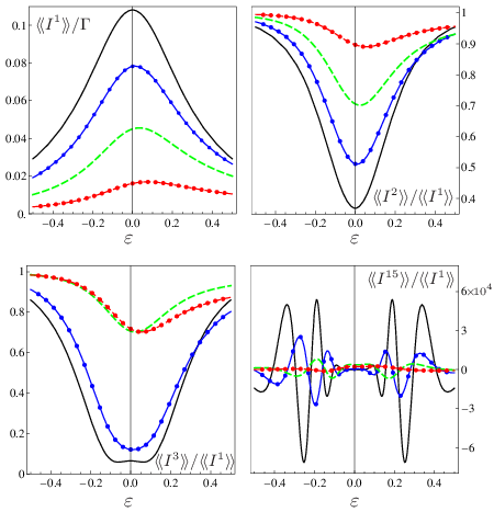
In Fig. 1 we show the first three cumulants of the current as functions of the level detuning $\varepsilon$ with different dissipations strengths $\alpha$. As an illustrative example the 15’th cumulant of the current, $\langle\!\langle I^{15}\rangle\!\rangle$, is also shown. As the dissipation strength is increased, a clear suppression of the coherent features (with $\alpha=0$) is seen. The increased coupling to the heat bath tends to localize the electron to one of the two quantum dots, thereby suppressing the effects of the coherent coupling between them. As a result a cross-over from coherent to sequential tunneling is observed with increasing $\alpha$. For large $\alpha$’s, the sequential tunneling process between the two quantum dots constitutes a ‘bottle-neck’ and the cumulants consequently approach the Poisson limit $\langle\!\langle I^{m}\rangle\!\rangle/\langle\!\langle I^{1}\rangle\!\rangle=1$, $m=1,2,3,\ldots$. The typical behavior of cumulants is, however, factorial growth, i.e., $|\langle\!\langle I^{m}\rangle\!\rangle|\approx c\,q^{m}\,m!$ for some constants $c,\,q>0$. In the coherent case ($\alpha=0$), this behavior is clearly seen for the 15’th cumulant, demonstrating its high sensitivity to dephasing and decoherence mechanisms.

Finite-frequency noise. The expression for the CGF, Eq. (2), allows us also to study the finite-frequency spectrum of the second cumulant of the current, the (symmetrized) current noise ²² 2 Non-symmetrized noise in a non-Markovian system was studied in Ref. [14], but not within the framework of FCS., expressed by MacDonald’s formula as $S_{II}(\omega)=\omega\int_{0}^{\infty}dt\sin{(\omega t)}\langle\!\langle I^{2}\rangle\!\rangle(t)$ [16, 17, 18], where $\langle\!\langle I^{2}\rangle\!\rangle(t)=\frac{d}{dt}\frac{\partial^{2}\mathcal{S}(\chi,t)}{\partial{(i\chi)^{2}}}|_{\chi\rightarrow 0}$. We then find

In order to evaluate this expression, we need to choose $\hat{\rho}(\chi,t=0)$ appropriately and find the inhomogeneity $\hat{\gamma}(\chi,z)$ as they enter the definition of $\langle\mathcal{G}(\chi,z)\rangle$. Following Ruskov and Korotkov [19] we assume that the system evolves from $t_{0}=-\infty$, such that the electronic occupation probabilities at $t=0$, where electron counting begins, have reached the stationary state, i.e., $\hat{\rho}(n,t=0)=\delta_{n,0}\hat{\rho}^{\rm stat}$. For this model the inhomogeneity is independent of the counting field [12]:

We see that the effects of the initial correlations accounted for by $\hat{\gamma}(z)$ vanish in the long-time limit. Moreover, since $\mathcal{W}\hat{\rho}^{\rm stat}=0$, we find $\langle\mathcal{G}(\chi,z)\rangle=\mathrm{Tr}\{\mathcal{G}(\chi,z)\mathcal{G}^{-1}(\chi=0,z)\hat{\rho}^{\rm stat}\}/z$ from which we can calculate the finite-frequency current noise. We note that only the proper inclusion of the inhomogeneity ensures a correct finite-time behavior, such as proper normalization of $\mathrm{Tr}\{\hat{\rho}(t)\}=\langle\mathcal{G}(\chi=0,t)\rangle=\mathrm{Tr}\{\hat{\rho}^{\rm stat}\}=1$ at all times.

Displacement currents (due to finite capacitances between quantum dots and leads) can be included in the finite-frequency current noise via the Ramo-Shockley theorem [20]. Evaluating the full current noise spectrum then requires an additional counting field accounting for tunneling from the left lead [18]. For the shown results we have included displacement currents and assumed identical capacitances between the left/right quantum dot and the left/right lead. In Fig. 2 we show the finite-frequency current noise $S_{II}(\omega)$ at frequencies around the hybridization energy $\Delta=\sqrt{\varepsilon^{2}+(2T_{c})^{2}}$, where signatures are expected in the current noise spectrum [7, 17, 20]. Resonances are not observed exactly at the ‘bare’ value $\omega=\Delta$, but are shifted towards lower frequencies. This renormalization occurs due to coupling to the heat bath which dresses the eigenspectrum of the electronic degrees of freedom, similar to the Lamb shift in atomic physics. The left figure shows how the signatures due to the coherent coupling between the two quantum dots are washed out with increasing temperature. In the right figure, we show how the frequency shift increases with increasing dissipation strength, which simultaneously reduces the effect of the coherent coupling. For larger $\alpha$’s ($\sim 0.1$) a change of line shape is observed (not shown).

In conclusion, we have presented a general theory for current fluctuations in non-Markovian quantum transport systems. Our methods allow us to calculate recursively zero-frequency current cumulants of very high orders, governed by a single dominating pole of the resolvent of the memory kernel, as well as the finite-frequency current noise, which is given not only by the resolvent, but also initial correlations. As an illustrative example of our approach, we have considered transport through a dissipative double quantum dot for which we have studied the effects of dissipation and temperature on the current cumulants of very high orders and the finite-frequency current noise.

We would like to thank R. Aguado, T. Brandes, S. Kohler, and K. Netočný for fruitful discussions and suggestions. The work was supported by FiDiPro, Italian MIUR via PRIN05, ESF (‘Arrays of Quantum Dots and Josephson Junctions’) and by the grant 202/07/J051 of the Czech Science Foundation.

References

- [1] Yu. V. Nazarov, ed., Quantum Noise in Mesoscopic Physics (Kluwer, Dordrecht, 2003).
- [2] B. Reulet, J. Senzier, and D. E. Prober, Phys. Rev. Lett. 91, 196601 (2003), Y. Bomze et al., Phys. Rev. Lett. 95, 176601 (2005), T. Fujisawa, T. Hayashi, R. Tomita, and Y. Hirayama, Science 312, 1634 (2006), S. Gustavsson et al., Phys. Rev. Lett. 96, 076605 (2006), A. Timofeev et al., Phys. Rev. Lett. 98, 207001 (2007), G. Gershon, Y. Bomze, E. V. Sukhorukov, and M. Reznikov (2007), eprint arXiv:0710.1852v1.
- [3] E. Sevick, R. Prabhakar, S. R. Williams, and D. J. Searles Annu. Rev. Phys. Chem. 59, 603 (2008).
- [4] D. A. Bagrets and Yu. V. Nazarov, Phys. Rev. B 67, 085316 (2003).
- [5] C. Flindt, T. Novotný, and A.-P. Jauho, Europhys. Lett. 69, 475 (2005a).
- [6] A. Braggio, J. König, and R. Fazio, Phys. Rev. Lett. 96, 026805 (2006).
- [7] R. Aguado and T. Brandes, Phys. Rev. Lett. 92, 206601 (2004a), Euro. Phys. Jour. B 40, 357 (2004b).
- [8] G. Kiesslich et al. , Phys. Rev. Lett. 99, 206602 (2007).
- [9] T. Speck and U. Seifert, J. Phys. A 38, L581 (2005), U. Seifert (2007), eprint arXiv:0710.1187v1.
- [10] R. Zwanzig, Nonequilibrium Statistical Mechanics (Oxford University Press, 2001).
- [11] Yu. Makhlin, G. Schön, and A. Shnirman, Rev. Mod. Phys. 73, 357 (2001).
- [12] C. Flindt et al. (to be published).
- [13] C. Flindt, T. Novotný, and A.-P. Jauho, Phys. Rev. B 70, 205334 (2004).
- [14] H.-A. Engel and D. Loss, Phys. Rev. Lett. 93, 136602 (2004).
- [15] S. A. Gurvitz and Ya. S. Prager, Phys. Rev. B 53, 15932 (1996).
- [16] D. K. C. MacDonald, Rep. Prog. Phys. 12, 56 (1949).
- [17] C. Flindt, T. Novotný, and A.-P. Jauho, Physica E 29, 411 (2005b).
- [18] N. Lambert, R. Aguado, and T. Brandes, Phys. Rev. B 75, 045340 (2007).
- [19] R. Ruskov and A. N. Korotkov, Phys. Rev. B 67, 075303 (2003).
- [20] Ya. M. Blanter and M. Büttiker, Phys. Rep. 336, 1 (2000).