Correlation of CMB with large-scale structure: I. ISW Tomography and Cosmological Implications
Abstract
We cross-correlate large scale structure (LSS) observations from a number of surveys with cosmic microwave background (CMB) anisotropies from the Wilkinson Microwave Anisotropy Probe (WMAP) to investigate the Integrated Sachs-Wolfe (ISW) effect as a function of redshift, covering . Our main goal is to go beyond reporting detections towards developing a reliable likelihood analysis that allows one to determine cosmological constraints from ISW observations. With this in mind we spend a considerable amount of effort in determining the redshift-dependent bias and redshift distribution () of these samples by matching with spectroscopic observations where available, and analyzing auto-power spectra and cross-power spectra between the samples. Due to wide redshift distributions of some of the data sets we do not assume a constant bias model, in contrast to previous work on this subject. We only use the LSS data sets for which we can extract such information reliably and as a result the data sets we use are 2-Micron All Sky Survey (2MASS) samples, Sloan Digital Sky Survey (SDSS) photometric Luminous Red Galaxies, SDSS photometric quasars and NRAO VLA Sky Survey (NVSS) radio sources. We make a joint analysis of all samples constructing a full covariance matrix, which we subsequently use for cosmological parameter fitting. We report a 3.7 detection of ISW combining all the datasets. We do not find significant evidence for an ISW signal at , in agreement with theoretical expectation in CDM model. We combine the ISW likelihood function with weak lensing of CMB (hereafter Paper II [1]) and CMB power spectrum to constrain the equation of state of dark energy and the curvature of the Universe. While ISW does not significantly improve the constraints in the simplest 6-parameter flat CDM model, it improves constraints on 7-parameter models with curvature by a factor of 3.2 (relative to WMAP alone) to , and with dark energy equation of state by 15% to [posterior median with “” (16th–84th percentile) range]. A software package for calculating the ISW likelihood function can be downloaded at http://www.astro.princeton.edu/˜shirley/ISW_WL.html.
pacs
98.80.Es, 95.36.+x, 98.65.Dx.I Introduction
The Cosmic Microwave Background (CMB) has provided us with a wealth of cosmological information. The large-scale anisotropies were first discovered by the Differential Microwave Radiometer (DMR) on Cosmic Background Explorer (COBE) satellite [2], and the smaller-scale CMB anisotropies were subsequently measured by various ground-based/balloon-borne experiments. More recently, the Wilkinson Microwave Anisotropy Probe (WMAP) satellite [3, 4] produced a cosmic variance limited map of CMB anisotropies down to . The structure of the angular power spectrum when combined with other cosmological probes (such as Sloan Digital Sky Survey, [5], Hubble Key Project [6] and 2dF Galaxy Redshift Survey [7]), allows extremely precise measurements of the cosmological parameters of the CDM model. While most of the fluctuations seen by WMAP and other CMB experiments were generated at the last surface of scattering, structures formed at low redshift also leave imprints on the CMB. These anisotropies, such as the thermal Sunyaev-Zeldovich (tSZ) [8] and kinetic Sunyaev Zeldovich effects (kSZ) [9], the Integrated Sachs-Wolfe (ISW) effect [10], and gravitational lensing, contribute only slightly to the CMB power spectrum on scales measured by WMAP, but they can be detected by cross-correlating the CMB with suitable tracers of the large scale structure.
This is the first of two papers that measure the Integrated Sachs-Wolfe effect and gravitational lensing (Paper II) in cross-correlation. In this paper, we focus on large scale galaxy-temperature correlations and their large scale cosmological source, the Integrated Sachs-Wolfe (ISW) effect. The ISW effect results from the red- or blue-shifting of the CMB photons as they propagate through gravitational potential wells. As the potential wells of the Universe (i.e., the spatial metric) evolve, the energy gained by photons falling into the potential well does not cancel out the energy loss as photons climb out of the well. This is important at late times when the Universe is not matter dominated and the gravitational potential is time dependent. It is only significant on large scales, since on small scales the amount of time spent by the photon in each coherence region of the gravitational potential is small and any small scale fluctuations will be smoothed out as the photon go through numerous potential wells along the line of sight.
To measure the above effect, we cross-correlate the CMB temperature anisotropies with maps of galaxies from the Two Micron All Sky Survey (2MASS), luminous red galaxies (LRGs) and quasars from the Sloan Digital Sky Survey, and radio sources from the NRAO VLA Sky Survey (NVSS). This incorporates most of the LSS tracers used by previous efforts [11, 12, 13, 14, 15, 16, 17, 18, 19, 20, 21, 22, 23, 24, 25] to detect the ISW effect. Our goal in this work extends this previous literature by going beyond detecting the ISW effect to measuring its redshift evolution and using that to constrain different cosmological models (e.g. the ISW effect due to spatial curvature occurs at significantly higher redshifts than that due to a cosmological constant). We therefore require a large redshift range ( to ) but with sufficient redshift resolution to unambiguously discern any redshift evolution of the signal. In addition, to draw robust cosmological conclusions from an observed redshift evolution, we must constrain both the redshift distribution and evolution of the bias with redshift for each of the samples; the simple assumption of constant bias is in most cases no longer sufficient. These considerations drive our survey selections; we discuss these in more detail in Sec. VIII. Our final product is a likelihood code that can be applied to any cosmological model. In addition to providing complementary constraints on standard cosmological parameters, we expect it can be a strong discriminator of the modified gravity models, which have very distinctive ISW predictions [26].
We review the theory behind the ISW effect in Sec. II. The CMB and LSS data sets used are described in Sec. III; the results of cross-correlating the two are in Sec. IV. Sec. V and VI constrain the redshift distributions of the samples, and possible systematic contamination of the cross-correlations. Sec. VII presents the cosmological implications of these results, and Sec. VIII summarizes our conclusions. The companion paper (Paper II) uses the same data sets to detect the weak lensing of the CMB. All of the theoretical predictions are made with WMAP 3 year parameters (=, = , , , ) except in Section V or otherwise stated.
II Theory
We briefly review the ISW effect and its cross-correlation with the galaxy density (see also Refs. [27, 28, 14]). The temperature anisotropy due to the ISW effect is expressed as an integral of the time derivative of the gravitational potential over conformal time ,
| (1) |
where and are the conformal time at recombination and today, respectively, and we ignored the effect of Thomson scattering suppression, which is negligible for the redshift range of interest here. For scales sufficiently within the horizon, the gravitational potential is related to the mass fluctuation in Fourier space by the Poisson equation:
| (2) |
where is the ratio of the matter density to the critical density today, is the Hubble constant today, is the speed of light, is the redshift, and is the comoving wave number. On large scales where the mass fluctuation , the perturbations grow according to linear theory = .
We are interested in cross–correlating the temperature anisotropies, , with the observed projected galaxy overdensity . The intrinsic angular galaxy fluctuations are given by:
| (3) |
where is an assumed scale-independent bias factor relating the galaxy overdensity to the mass overdensity, i.e. , is the normalized selection function, and is the comoving distance to redshift . We focus on the cross-spectrum of the galaxies with the CMB temperature fluctuation:
| (4) |
where is the matter power spectrum today as a function of the wave number , and the functions and are
| (5) |
and
| (6) | |||||
The Limber approximation, which is quite accurate when is not too small (), can be obtained from Eq. (4) by setting and using the asymptotic formula that (when ). We find that the substitution is a better approximation to the exact expressions than . This gives
| (7) | |||||
The above discussion ignores the effects of gravitational lensing, which alters the expected signal through two competing effects – changing the flux limit of the survey as well as the observed galaxy density. Both of these effects can be thought of as altering the redshift distribution of the tracers, and so we defer the discussion to Sec. V.
III Data
We describe the CMB and galaxy data sets used in our analysis below; these are summarized in Table 1. The data sets not used in this paper are discussed further in the Sec. VIII, where we provide detailed explanations for the choices made. All large scale structure data were pixelized in the HEALPix system with the resolution and sky coverage shown in Table 1.
| Sample (its notation in paper) | Area | Density | Number of | HEALPix | Number of | |||||||||
|---|---|---|---|---|---|---|---|---|---|---|---|---|---|---|
| deg2 | deg-2 | galaxies | resolution | HEALPix Pixels | ||||||||||
| 2MASS, (2MASS0) | 27 191 | 01.84 | 0 050 096 | 09 | 073 457 | 1.63 | 0.06 | |||||||
| 2MASS, (2MASS1) | 27 191 | 03.79 | 0 103 060 | 09 | 073 457 | 1.52 | 0.07 | |||||||
| 2MASS, (2MASS2) | 27 191 | 07.85 | 0 213 516 | 09 | 073 457 | 1.54 | 0.10 | |||||||
| 2MASS, (2MASS3) | 27 191 | 16.00 | 0 435 570 | 09 | 073 457 | 1.65 | 0.12 | |||||||
| SDSS, LRG, low- (LRG0) | 06 641 | 35.10 | 0 232 888 | 10 | 025 731 | 1.97 | 0.31 | |||||||
| SDSS, LRG, high- (LRG1) | 06 641 | 93.80 | 0 622 646 | 10 | 025 731 | 1.98 | 0.53 | |||||||
| SDSS, QSO, low- (QSO0) | 06 039 | 20.80 | 0 125 407 | 10 | 842 044 | 2.36 | 1.29 | |||||||
| SDSS, QSO, high- (QSO1) | 06 039 | 18.30 | 0 110 528 | 10 | 842 044 | 2.75 | 1.67 | |||||||
| NVSS point sources (NVSS) | 27 361 | 40.30 | 1 104 983 | 08 | 0521 594 | 1.98 | 1.43 |
III.1 CMB temperature from WMAP
The WMAP mission [3, 4] measured the all-sky maps of the CMB at multipoles up to several hundred. We use the second public data release of the WMAP data with the first three years of observations. The all-sky CMB maps are constructed in the following bands: K (23 GHz), Ka (33 GHz), Q (41 GHz), V (61 GHz) and W (94 GHz). These maps are pixelized in the HEALPix [29] resolution 9 format with pixels, each 47.2 sq. arcmin in area. These maps are not beam-deconvolved and this, with the scan strategy of WMAP, results in nearly uncorrelated Gaussian uncertainties on the temperature in each pixel [4]. We limit our analysis to Ka through W band as the K-band is heavily contaminated by the Galactic emission. We trim all masks with the WMAP Kp0 mask and point source mask to remove regions contaminated by Galactic emission and point sources, leaving 76.8% ( resolution 9 HEALPix pixels) of the sky for the ISW analysis. We choose not to use either the WMAP “Internal Linear Combination” (ILC) map or the foreground cleaned map to avoid a number of practical difficulties as these maps lose frequency dependence of the original maps and have complicated pixel-pixel noise correlations.
III.2 Two Micron All Sky Survey (2MASS)
We use galaxies from the Two Micron All Sky Survey (2MASS) Extended Source Catalog (XSC) [31, 30, 32] as mass tracers of the low redshift Universe. The median redshift of these objects is . We use , the -band isophotal magnitude measured inside a circular isophote with surface brightness of 20 mag arcsec-2, as our default flux measure. We extinction correct the magnitudes from the catalog using the reddening maps [33]:
| (8) |
where [14]. Note that we ignore changes to the isophotal radius due to extinction. We remove regions with in the dataset as the galaxy density starts to drop drastically. We visually inspects how the galaxy density changes with and decide to cut with as there is a drastic drop. There are galaxies in the 2MASS XSC after removing known artifacts and sources in close proximity to a large galaxy (’a’ and ’z’) and requiring (which rejects duplicate observations of the same part of the sky). The 2MASS XSC can miss objects near bright stars or overlapping artifacts, and so we used the XSC coverage map [30] and masked out pixels with coverage, thus of the sky.
We divided the 2MASS sample into 4 flux bins: , , , . Note that the redshift distribution of these 4 bins actually overlap significantly. Our sample selection for 2MASS is similar to Afshordi et al. [14] except the pixelization.
III.3 Data from Sloan Digital Sky Survey (SDSS)
The Sloan Digital Sky Survey has taken CCD images of deg2 of the high-latitude sky [34]. A dedicated 2.5m telescope [35, 36] at Apache Point Observatory images the sky in photometric conditions [37] in five bands () [38, 39] using a drift-scanning, mosaic CCD camera [35]. All the data processing are done by completely automated pipelines, including astrometry, source identification, photometry [40, 41], calibration [42, 43], spectroscopic target selection [44, 45, 46], and spectroscopic fiber placement [47]. The SDSS is well underway, and has produced seven major releases [48, 49, 50, 51, 52, 53, 54].
In addition to constructing LRG and quasar maps, we constructed three additional maps that we use to reject region sheavily affected by poor seeing or stellar contamination. These include (i) a map of the full width at half-maximum (FWHM) of the point-spread function (PSF) in band; (ii) a map of stellar density ( stars, smoothed with a 2 degree FMHM Gaussian); and (iii) a similar map using only the red stars ().
All SDSS magnitudes used here are extinction-corrected using the maps of Ref. [33]. We use SDSS model magnitudes for the LRGs, and PSF magnitudes for the quasars and stars.
III.3.1 Luminous Red Galaxies
We use the photometric Luminous Red Galaxies (LRGs) from Sloan Digital Sky Survey (SDSS) constructed as described in [55]. The LRGs have been very useful as a cosmological probe since they are typically the most luminous galaxies in the Universe, thus probing a larger volume than most other tracers. On top of this, they also have very regular spectral energy distributions and a prominent 4000Å break, making photo- acquisition much easier than the other galaxies. We will not be repeat our selection criteria here as it is thoroughly described in [55]. We only accept sky regions with (almost identical to as in [55]) and an band FWHM arcsec.
Furthermore, there are a few regions in SDSS that have 60% more red stars than typical for their galactic latitude; we suspect photometric problems and rejected these regions. The red star cut removed deg2 in assorted parts of the sky.
We slice our LRG sample into two redshift bins for the ISW analysis: and .

III.3.2 Photometric quasars
We select quasars photometrically from the Sloan Digital Sky Survey by first generating a candidate quasar catalog consisting of UVX objects [56]. These are point sources with excess UV flux (i.e. ) observed magnitudes fainter than 14.5 (to avoid saturation problems), extinction corrected magnitudes brighter than , and u-band error less than mag ( detection in ). We call this the ALL-UVX catalog. We also have the public catalog of photometric quasars from Data Release 3 (DR3) generated by Ref. [57], which we will call DR3-QSO objects. We also construct a UVX object list from only DR3 data, denoted DR3-UVX. This catalog is used to extend the selection and photometric redshifts from the DR3 region to the ALL region. Ideally the catalog would have been based on running the algorithm of Ref. [57] on the ALL region but this option was not available at the time we constructed the quasar catalog.
We first match the DR3-UVX objects to the DR3-QSO objects and then assign the photometric redshifts from the DR3-QSO objects to the matched DR3-UVX object. For objects that are in DR3-UVX catalog, but not in the DR3-QSO catalog, we mark them as rejects. We now have a DR3-UVX catalog with every object either assigned a redshift or marked as a reject. The reject rate for DR3-UVX (ALL-UVX) is (). Then, we lay down the DR3-UVX catalog in color4 (,,,) space, and then for each ALL-UVX object, we find its nearest neighbor in this color4 space, then assigning it the same “redshift” as its matched DR3-UVX neighbor. If the DR3-UVX object has a redshift (not a reject), then the ALL-UVX object is classified as a quasar with the same redshift (photo- only), otherwise it is rejected. This procedure generates a photometric catalog of quasars in the full survey area, based on the matching against DR3 quasars in color4 space. However, this catalog only has the photometric redshifts, but not the actual redshift distribution. The actual redshift distribution will be discussed in Sec. VI. The average color offsets of the quasar candidate to its match for , , and are , , and , while the typical errors on the colors of the candidates are (), (), () and (). As the color differences between the match and the candidate are well within the error of the colors, we conclude that the quasar candidates are matched with high accuracy.
We then cut the catalog according to and FWHM arcsec. These cuts are determined when we look at the variation of the quasar number overdensity over a range of extinction and seeing. Also, since quasars are more sensitive than LRGs to extinction (as a result of the importance of the filter in selecting quasars), we cut the catalog at a lower . We also imposed a cut rejecting regions with more than twice average stellar density, i.e. we require stars/deg2.
We further divide the sample into two redshift (photo-z) bins: (low-) and (high-). This division of sample is due to the fact that there are strong emission lines (e.g. Mg ii) that redshift from one filter into the next around the redshifts of , and , causing these two redshift bins to be relatively free of cross-contamination. However, as we will see, they do contain significant contamination from redshifts below and above . We therefore constrain their redshift distribution by cross-correlating these with auxiliary data sets; we discuss this further in Sec. V.
The construction of the full sample using the DR3 catalog as described above introduces one potentially worrying systematic, namely the possibility that regions of the sky observed after DR3 would have a different density of sources than DR3 regions as a result of the nearest-neighbor method misbehaving in low-density regions of color4 space. This would provide a spurious feature in the quasar maps that resembles the DR3 coverage map. In order to check for this problem, we look for correlations between observing dates (if the ALL sample is misbehaving, it will be different from DR3 sample) with galaxy overdensity, and we do not find any significant correlations (Fig. 2). We also look at the correlation between quasar overdensity and the stellar number density to see if there is significant stellar contamination, we do not find any either (Fig. 2).

III.4 NRAO VLA Sky Survey (NVSS)
The NRAO VLA Sky Survey (NVSS) is a 1.4 GHz continuum survey covering the entire sky north of declination using the compact D and DnC configurations of the Very Large Array (VLA) [58]. The images all have 45 arcsec FWHM resolution and nearly uniform sensitivity and yield a catalog of almost discrete sources stronger than mJy.
This survey has several potentially major artifacts: Galactic synchrotron emission, spurious power from bright sources and a declination-dependent striping problem. All of these have to be treated properly before one can claim that the power coming from the cross-/auto-correlation is not due to some spurious issues. The Galactic synchrotron emission can in principle be an issue because it contributes significantly to the noise temperature of the VLA, and for realistic number counts, increased noise temperature could change the number of sources with measured flux above some threshold. (As an interferometer the VLA is not directly sensitive to the diffuse synchrotron foreground.) This issue is treated by incorporating a template – the Haslam map [59] – in the cross-correlation analysis and projecting out the power that are correlated to this template. Even though the Haslam map is at 408 MHz, the frequency dependence of the galactic synchrotron emission is fairly flat, allowing us to use it as a template of the Galactic synchroton radiation. The bright sources are problematic since the VLA has a finite dynamic range ( in snapshot mode with limited -plane coverage) and thus the identification of faint sources in fields with a bright source is unreliable. This issue is mitigated by masking out all the bright sources. Striping is a known systematic effect in NVSS [60]: the galaxy density has a systematic dependence on declination, which can mimic long-wavelength modes in the galaxy field. To deal with the above potential problems, we first impose a flux limit of 2.5 mJy (where NVSS is 50% complete), mask out a 0.6 degree radius around all the bright sources ( Jy). Then to reduce striping, we also include templates to project out the synchrotron and declination-striping modes. The implementation of this projection of spurious power will be further discussed in Sec. IV.
IV Cross-correlation power spectrum analysis
IV.1 Methodology
We start by organizing the temperature fluctuations and the galaxy overdensities into a single data vector,
| (9) |
where is a vector with the measured CMB temperature (with the monopole and dipole subtracted) in band at every HEALPix pixel; analogously, is the tracer number overdensity. The vector has a total length where and are the number of accepted pixels for the CMB and LSS maps respectively. We suppress the band subscript for simplicity, with the implicit understanding that we always refer to the cross correlation of a single WMAP band with the tracer overdensity. The covariance matrix of is,
| (10) |
where is given by,
| (11) |
where is the noise matrix. The submatrices , and are defined by
| (12) |
where is the position (on the sky) of the point of the vector . The temperature-temperature, galaxy-galaxy and galaxy-temperature angular power spectra are denoted by and respectively.
The galaxy power spectrum is first estimated using a pseudo- estimator [61], and fit by the non-linear power spectrum of [62], multiplied by a constant linear bias. We project out the monopole and dipole of both these power spectra by setting the power in the modes to a value () much greater than the true power spectrum.
We parametrize as a sum of bandpowers, , with amplitudes to be estimated,
| (13) |
We consider “flat” bandpowers given by
| (14) |
where is the product of the beam transfer function [63], and the HEALPix pixel transfer functions at WMAP and LSS resolution. This parametrizes the power spectrum as a sum of step functions and is useful when the shape of the power spectrum is unknown.
We estimate the by forming quadratic combinations of the data [64, 65],
| (15) |
These are related to the estimated by the response matrix ,
| (16) |
where
| (17) |
If , then the are good approximations to the maximum likelihood estimates of the . The covariance matrix of the is the inverse of the response matrix, if the fiducial power spectra and noise used to compute correctly describe the data (in this case is the Fisher matrix, hence the notation). The matrix determines the weighting and is often called a “prior” in quadratic estimation theory. Note that this usage has nothing to do with Bayesian priors – in particular, Eq. (16) is unbiased regardless of the choice of prior (though for bad choices the estimator is not minimum variance). Implementing the above algorithm is complicated by the sizes of the datasets; the implementation we use is in [66, 67, 18], and we refer to the reader to the discussion there.
[In addition to the cross-power spectra in Eq. (14), in quadratic estimator theory one usually tries to estimate the CMB and galaxy auto-power spectra as well. Because our prior is diagonal, however, these decouple, i.e. the entries in that couple the auto-powers and cross-powers are zero. For this reason we can leave the auto-powers out of the quadratic estimator.]
As mentioned earlier, the NVSS dataset has issues that require additional processing. Assume a systematic that we characterize as follows:
| (18) |
If estimate , even if is the true covariance, we will still have a biased answer. However, the substitution
| (19) |
yields an unbiased estimate of when . One can add as many systematic templates (i.e. modes to project out of the map) as desired. To immunize the NVSS correlations from possible systematics, we break the NVSS map into 74 declination rings, and for each ring include a template map consisting of either (for pixels within the declination ring) or (for all other pixels). This removes the declination-dependent stripes. We also put in the 408 MHz Haslam map [59] (technically K) as a template for the Galactic synchrotron radiation. We experimented with the values of and found that the cross-spectra are converged with the choice for the declination rings and K-2 for the synchrotron map.
IV.2 Priors
To generate the priors for the cross-correlation power spectrum analysis, we need the approximate autopower spectrum of the galaxies. The auto-correlation is done using the same methodology as described in Sec. IV.1. The resulting autopower spectra must be smoothed, before being used as priors. This avoids statistical fluctuations in over- or under-weighting the corresponding monopoles in the cross-correlation, which could result in underestimation of signal since we would artifically down-weight multipoles that had accidentally high power in galaxies and place more weight on multipoles that had little power. We did the smoothing in two different ways. For the cases where the redshift distribution was available early enough in the analysis (2MASS or LRG), we fit the auto-power spectrum to the non-linear matter power spectrum [62] to get the linear bias. In other cases (quasars, NVSS) we did not have the redshift distribution at the time the priors were created; we created the priors by using a smoothed, splined auto-power spectrum of the sample as the prior.
In the cases where we did a fit using the nonlinear matter power spectrum, the fit biases are 1.15, 1.18, 1.20, and 1.22 (2MASS, brightest to faintest); 1.92 (LRG low-); and 1.86 (LRG high-). After generating the priors, we made several modifications to the analysis, including the inclusion of redshift-dependent bias in 2MASS. Thus while the priors were not updated since they give a good fit to the observed autopower spectrum, it should be noted that these bias values are not used in the cosmological analysis (i.e. for ISW prediction purposes).
To generate priors for the CMB, we generate the priors using the theoretical s from WMAP and take into the account of the effect of pixelization and beams by convolving with the pixel and beam window functions.
IV.3 Results of cross-correlation


Figs. 3, 4, and 5 plot the cross-correlation between WMAP and the 2MASS, SDSS and NVSS samples respectively; the four different symbols in each of these plots correspond to the four WMAP bands we use. The observed achromatic nature of the signal is consistent with it being ISW, and is an important check for frequency dependent systematics. The two quasar samples are at the highest redshifts we can probe, so if there is an ISW cross-correlation at –2, it would mean that there is significant gravitational potential change at these redshifts. This is not expected in simplest CDM cosmology, but could be present either in models where dark energy equation of state is rapidly changing with redshift or in models where curvature plays a role. The observed lack of a signal for these redshifts therefore strongly constrains such models. Note however that the NVSS cross-correlation cannot be automatically interpreted as a detection of high redshift ISW, as (see below) it covers a wide redshift range.

V Redshift Distributions
The basic problem is to determine for each galaxy sample and each cosmological model the function that relates the matter density to the two-dimensional galaxy overdensity :
| (20) |
Eq. (20) is understood to be valid on scales where the galaxies trace the matter distribution. In the absence of magnification bias, the function is simply the product of the bias and the redshift distribution: , where is the probability distribution for the galaxy redshift. In the presence of magnification bias, which is important for the SDSS quasars and possibly the NVSS radio sources, takes on the more complicated form
| (21) |
where is the slope of the number counts of the galaxy density as a function of flux: . Here is the lensing window function:
| (22) | |||||
where is the radial comoving distance, is the sine like function (equal to in a flat Universe), and is the cotangent like function (equal to in a flat Universe).
It is in fact the function that is required if one is to predict the ISW effect in a given cosmology. It is this same function that is required to predict the linear-regime angular power spectrum of the galaxies. This section describes the method by which is obtained for each of the samples. The methods are quite different due to the different types of information available for each sample. In particular there are very few spectroscopic redshifts available for NVSS. Note however that all methods include galaxy clustering data, as this is needed to determine the bias even if the redshift probability distribution is known perfectly.
All of the numbers and plots in this section only that depend on cosmology are computed using the original WMAP third-year flat 6-parameter CDM cosmology (, , , , and ), i.e. from the first release of Ref. [68]. However in the Markov chain, the functon is re-computed for each cosmological model and used to predict the ISW signal.
V.1 2MASS
The 2MASS samples go down to a limiting magnitude of . At this relatively bright magnitude, almost all objects (97.9%, after correcting for the fiber collisions) have SDSS spectra, provided of course that they lie within the spectroscopic mask. In practice there are two subtleties that can occur. One is that the bias cannot be obtained to high accuracy from linear theory because even the moderate multipoles () are nonlinear, especially for the nearest 2MASS slice, and the lowest multipoles suffer from cosmic variance. The other is that the bias varies with redshift: even though the 2MASS galaxies cover a narrow range in redshift during which the Universe expands by only %, the use of apparent magnitude to define the samples means that the typical luminosity of a galaxy varies by several magnitudes across the redshift range of interest. more biased, this effect shifts the peak of the effective redshift distribution to higher redshifts than the actual distribution .
We match the 2MASS galaxies with the SDSS MAIN galaxy sample by first defining the 2MASS sample as discussed in III.2, then we select 2MASS galaxies only within mask that is more than 90% complete. We then try to match all the 2MASS galaxies with the SDSS MAIN galaxies that are within and found that almost all of the objects from 2MASS sample have SDSS spectra. We thus use the spectroscopic redshifts of the matched SDSS galaxies to identify the redshifts of the 2MASS galaxies. The redshift distribution is binned with . The redshift distribution for each of the four slices is shown in Fig. 6.

The problem of nonlinear evolution is generally very complicated, however for ISW work we only need a solution accurate to a few tens of percent. Therefore we have used the -model [7], which relates the galaxy power spectrum to the linear power spectrum via
| (23) |
where is the linear bias appearing in Eq. (21). Cole et al. [7] found in simulations that this function fits the galaxy power spectrum in simulations for Mpc, while the required value of varies depending on the sample. Our method is to compute the theoretical angular galaxy power spectrum via the Limber integral, and fit this to the measured treating and as free parameters. This procedure can be done either assuming is constant with redshift, or (better) taking into account the redshift-dependent bias,
| (24) |
where is known and is a free parameter. While there is very little evolution in the 2MASS redshift range, the nearby and distant galaxies can have very different biases because they correspond to different luminosity ranges. The results for each are shown in Table 2. is based on taking the r-band luminosities of the galaxies and using from Tegmark et al. [5]. Note that the prominent peak of redshift distribution at is a supercluster known as the Sloan Great Wall. (In principle can depend on redshift as well, so one should be careful about interpreting the fit value and indeed one can see from Table 2 that fit in this way is not stable. However the changes in seen in the table when we restrict to much lower suggest that this is not a large effect on the bias.)
| range | Varying fit | Constant fit | fit | |||||||
|---|---|---|---|---|---|---|---|---|---|---|
| 12.0–12.5 | 49 | |||||||||
| 12.5–13.0 | 61 | |||||||||
| 13.0–13.5 | 74 | |||||||||
| 13.5–14.0 | 99 | |||||||||
The -model fits for the 2MASS sample (and the LRGs) are shown in Fig. 7.

V.2 SDSS LRGs
Next we consider the photometric LRG sample from SDSS. The sample is faint enough that spectroscopic redshifts are unavailable for most of the objects. Fortunately, precise photometric redshifts are available for LRGs since they have very uniform spectra whose main broadband feature is a break at 400 nm. This break passes through the SDSS and filters in the interesting redshift range, so the and colors of an LRG correlate very strongly with its redshift [55]. The error distribution of the photometric redshifts has been calibrated using spectro-s from the 2SLAQ survey[69]; this procedure, and an inversion method used to determine the actual redshift distribution given the photo- distribution, are described in Padmanabhan et al. [55]. These methods were applied to determine the redshift probability distribution for the LRGs used in this sample. The redshift distributions so obtained are shown in Fig. 8.

The bias is determined by the same -model fitting procedure as we used for 2MASS. The maximum values of considered are 240 for the low- slice and 400 for the high- slice, which correspond to roughly Mpc-1 at the typical redshifts of these samples. For the fiduciual cosmology, the low- LRG slice gives a bias of and ; the high- slice gives and . In order to reduce the possible impact of the nonlinear regime on our results, we also did fits where the maximum value of was reduced by a factor of 2 or 4. The results are shown in Table 3 and the bias estimates are seen to be consistent with each other. In what follows we have used the original () fits for the LRG bias, noting that the remaining uncertainty in is small compared to the uncertainty (change in number of sigma detection is: 0.0043 (0.0388) for low-z LRG (high-z LRG)) resulting from statistical error in the ISW signal. However we note that it is not clear how well the -model works for LRGs at small scales, and we recommend more detailed analysis before taking the very small statistical error in at face value. The -model fits are shown in Fig. 7.
| Value of | Low- slice | High- slice | ||
|---|---|---|---|---|
For the LRGs – unlike the 2MASS galaxies – each of the two photo- slices covers a narrow redshift range and the threshold luminosity varies slowly across that range, so we expect the bias to not vary significantly across the redshift range. This expectation has been confirmed in previous angular clustering studies which found % variation from to [70], and also by our own bias analysis which finds no significant difference between the two bins. Thus we conclude that for the purposes of ISW work (where we have a sigma signal for low-z LRG (high-z LRG) correlation), variation of the LRG bias within an individual photo- bin (0.2–0.4 or 0.4–0.6) can be neglected.
We calculate the possible contribution from magnification bias given the redshift distribution of the LRGs and also an assumed cosmology. We find that the possible contribution from magnification bias is times (depending on the scale) smaller than the actual signal. Therefore magnification bias is not contributing significantly to our signal.
V.3 SDSS quasars
The function for the quasars is more uncertain than for the LRGs. This is in part due to the limited spectroscopic coverage available, but also the difficulty of constructing quasar photo-s and the lower clustering amplitude, which leads to noisier estimates of bias parameters. The basic procedure for obtaining is thus to find a region of sky with as high spectroscopic completeness as possible while still retaining a large area; use this to obtain a preliminary estimate ; and then fit for the bias parameters using clustering data, of which several are needed if is multimodal. The remainder of this section describes the details of the determination and what possible errors can be introduced by spectroscopic incompleteness, stellar contamination, redshift-dependent bias, and cosmic magnification.
In order to determine the redshift probability distribution, we began by constructing a set of five rectangles that lie within the coverage area of the
SDSS, 2QZ [71], 6QZ [71], and 2SLAQ [72] surveys. These rectangles lie along the equator (the declination range is
to ) and cover the five RA ranges 137–143∘, 150–168∘, 185–193∘, 197–214∘, and
218–230∘. There is a significant amount of area with coverage from all surveys that is rejected as it was found to have lower completeness in
2SLAQ because there is less plate overlap. Spectra in SDSS were required to have high confidence (zConf) [48] and those in
2QZ, 6QZ, and 2SLAQ were required to be of high quality (quality) [71].
Our coverage rectangles contained a total of 1410 low-redshift and 1269 high-redshift photo- quasars; these numbers are lower than the product of the spectroscopic coverage area and the number density of photo- quasars because some parts of the latter catalogue were rejected by our stellar density cuts. Of the low-redshift photo- quasars, we found that 257 (18%) had no spectroscopic redshift determination or low quality ones, 58 (4%) were identified as stars, and the remaining 1095 (78%) are extragalactic. For the high-redshift sample these numbers are 208 (16%), 13 (1%), and 1048 (83%) respectively. From this data we construct a preliminary redshift probability distribution for each of the photo- slices using a kernel density estimator,
| (25) |
where is the number of matches to extragalactic objects, is the redshift of the th object, and is the kernel width. The estimator is consistent in the limit that the number of objects and at fixed . In practice, must be chosen to be small compared to the width of any real features in the redshift distribution (otherwise these are artificially smoothed out), and large enough to smooth out shot noise (and redshift-clustering noise, if significant). We have used (using changes the fit bias by only 5%). This preliminary distribution is shown in the top panel of Fig. 9. The redshift distributions in the two photo- quasar slices are multimodal due to the nature of the photo- error distribution: the quasar spectra redward of Lyman- are usually characterized by a roughly power-law continuum with superposed emission lines. This means that quasar colors oscillate as emission lines redshift into and out of the SDSS filters, resulting in an (approximately) self-intersecting locus in color space and many degeneracies in the photo- solution.

If the quasar bias were constant and magnification bias negligible, then we would have simply , with the proportionality constant being the product of the bias and the probability for a photo- quasar to actually be extragalactic. This constant could then be determined by fitting the amplitude of the quasar autocorrelation function, as has been done in most past ISW studies. However, in the real Universe quasars are known to have an evolving bias, which is potentially significant across the redshift range considered, and at redshifts lensing magnification can become significant. The magnification can be calculated from the slope of the quasar counts near the magnitude limit, which gives for the low- sample and for the high- sample. In principle the cut on the -band magnitude error () could have an additional effect since magnification will reduce ; however this is not an issue for us since at the threshold, for UVX objects we will have where the typical magnitude error is even accounting for extinction (). Since for these samples is small, we compute the magnification bias using in place of the true distribution . That is, we replace Eq. (21) with
| (26) | |||||
This leaves only the problem of constraining the product using the clustering data, i.e. the quasar power spectrum and quasar-LRG cross-power. Unfortunately the data is not capable of constraining a full model-independent distribution, so instead we write
| (27) |
where is the growth factor, and is a piecewise constant function of . This is equivalent to assuming that the clustering amplitude (divided by spectroscopic completeness) of the quasars is constant in redshift slices, which has been found to be a better approximation than constant bias in most quasar surveys [73]. For comparison, the empirical “Model 3” of Ref. [74] predicts to change by only 5% from to 1.45, and by 13% from to 2.00. For the more recent model, Eq. (15) of Ref. [75], these numbers are 24% and 15% respectively. At higher redshifts () there is a sharp increase in [76] but UVX-selected samples do not contain objects from this redshift range.
We constrain in as many redshift slices as can be constrained using the data. In particular since the quasar redshift distributions are multimodal, we would like to be able to fit a different clustering amplitude in each peak. The treatment of the two quasar samples is slightly different due to the availability of different information in their redshift ranges, so we now discuss their redshift distributions separately. In each case, the autopower spectra were fit to linear theory up to (Mpc-1 at ) and the quasar-LRG cross-spectra were fit up to (Mpc-1 at ).
V.3.1 Low- sample:
For the low- quasar sample, we can only constrain one redshift slice. An examination of Fig. 9 shows that the distribution is actually trimodal, with peaks at , , and . A fit assuming a constant yields , with dof (). Almost all of the weight for this comes from the central () peak. We also ran two-slice fits to determine whether the clustering data constrain the amplitudes of the low- and high-redshift peaks. The first such fit is of the form
| (28) |
which allows the low-redshift slice to vary ( is the local minimum of ). This fit gives and , with dof. We also tried a two-parameter fit in which the high-redshift slice is allowed to vary:
| (29) |
(the local minimum of between the main and high-redshift peaks is at ). This fit gives and (), with dof. The errors on are highly asymmetric in this case because the constraint comes mainly from the quasar autopower; and are then degenerate because one only knows the total power, not how much comes from each redshift slice. The shape of the power spectrum breaks this degeneracy in principle, however in practice it is far too noisy. The fact that the high-redshift slice cannot give negative power accounts for the “hard” upper limit on .
From this exercise we conclude that the clustering data cannot independently measure the bias in either the low- or high-redshift peak. The reasons are different in each case. The low-redshift peak contained only 1.7% of the spectroscopic identifications, and thus almost certainly contains only a very small fraction of our quasars. This peak lies at the same redshift as the low- SDSS LRGs, and the quasar-LRG cross-correlation is the major constraint on . Unfortunately this cross-correlation is drowned out by the enormous Poisson noise contributed by the quasars in the other two peaks, and is detected at only . On the other hand, the LRGs oversample the cosmic density field on linear scales and cover the same region of sky as the quasars. One would thus expect that since the LRG-quasar correlation is only seen at this low significance, and the ISW effect from this redshift range contributes only a small fraction of the power in the CMB, the contribution of the low-redshift peak to the quasar-ISW correlation would be statistically insignificant. We find that the predicted peak of the quasar-ISW for only the low-redshift peak quasars is lower than the entire sample (high-z QSO) by , which is significantly smaller than the error on the cross correlation. This is run using a WMAP-3yr parameters.
The high-redshift peak contains 10% of the quasars. Its amplitude must be measured in autocorrelation due to the lack of other samples at that redshift, which is a serious drawback since only 1% of quasar pairs come from the high-redshift peak. An alternative approach to constraining its amplitude would be cross-correlation against the spectroscopic quasar sample at , but we did not pursue this approach here.
V.3.2 High- sample:
The high- photometric quasar sample also has a trimodal distribution: there is one peak at , a second at , and a third at . In this case however, it is the highest-redshift peak that contains most of the objects, with the middle peak in second place and only a few objects in the lowest-redshift peak. This situation makes it both possible and necessary to fit separate amplitudes for the peaks; in this case we will find that two amplitudes can be constrained, one for the two low-redshift peaks and one for the main (high-redshift) peak.
As a first step, we attempt to fit all three of the peaks with separate amplitudes,
| (30) |
This leads to the results , , and (1), with dof. The large error bar on indicates that this parameter cannot be constrained from the data, so we instead try a two-slice fit in which we fix . This fit gives the tighter constraints and , with dof, and it is what we use for the rest of the paper.
V.3.3 Redshift Distribution Summary
The quasar autopower spectra and quasar-LRG cross-spectra, along with the model fits, are shown in Fig. 10. For the QSO0 sample, there is excess power ( above the prediction) in the lowest- bin, corresponding to a % RMS fluctuation in the number density on scales of degrees. The two most obvious sources of such power are stellar contamination and photometric calibration errors. Given that % of the photometric “quasars” are actually stars [56] and that the relative photometric calibration across the sky in SDSS is estimated to be % in the band (the worst band, but one very important for quasar work) [70], either of these seems plausible. In any case, these very low multipoles were not used in fitting the redshift distribution in either auto- or cross-power.

It is essential to test the robustness of the quasar fits, in particular against the possibility of nonlinear clustering affecting the range of multipoles used in the fits. The first way we do this is by repeating our analysis using the nonlinear matter power spectrum of Smith et al. [62] in place of the linear power spectrum. In the analysis with the nonlinear spectrum, the amplitude for the low- quasar slice increases by , and the amplitudes for the and parts of the high- quasar slice increase by and , respectively. If we restrict our attention to the lowest multipoles (instead of cutting at 140 or 160), these changes are , , and . In each case the change is very small compared with the error bars. Thus we do not believe that nonlinear clustering is affecting our estimates.
V.4 NVSS
The function for NVSS is the hardest to obtain because there are no spectroscopic samples of NVSS objects that have sufficiently high completeness to obtain the redshift distribution. Past ISW analyses [15, 17] with the NVSS have been based on the radio luminosity function of Dunlop & Peacock [77], which itself was fit to a combination of source counts, redshifts for some of the brightest sources, and the local luminosity function. A constant bias was then assumed. The redshift distribution so obtained is reasonable, however it has three major drawbacks: (i) the redshift probability distribution for the faint sources (which make up most of the sample) is constrained only by the functional form used for the luminosity function and not by the data; (ii) it does not give the redshift dependence of the bias, which could be very important since the redshift range is broad, and the typical luminosity of the sources varies with redshift; and (iii) the absolute bias is constrained using the NVSS autopower spectrum, which is known to contain power of instrumental origin and hence is probably a less reliable constraint than the cross-correlation against other surveys. The alternative method to measure is by cross-correlation against the other samples whose redshift distributions are known. This method is adopted here, since it does not have any of the aforementioned problems. Its main drawback is that the other samples only probe the range out to , and little data is available to constrain above that.
V.4.1 Procedure
In order to measure the effective redshift distribution of NVSS, we must first obtain the cross-correlation of NVSS with each of the eight other samples (the four 2MASS samples, and two samples each of LRGs and quasars). This is done by using the same angular cross-spectrum estimation method as was used for the ISW analysis, and the cross-spectra are shown in Fig. 11. The main subtlety that arises is that the cross-spectrum (where and are LSS samples) can actually contain Poisson noise if there are objects that are in both samples. The Poisson noise term is of the form
| (31) |
where is the number of sources per steradian in catalog , and is the number of sources per steradian that appear in both catalogs. In order to measure we must match the NVSS to each of the other samples. Note that the positional errors in NVSS are typically several arc seconds, and consequently there will always be some false matches. Therefore we estimate the fraction of matches as
| (32) |
where is the number of matches within some radius , and is the number of sources in catalog in the NVSS mask. This was estimated for radii of 40 and 20 arcsec, and the results are shown in Table 4.
| Sample | Multipoles used | ||||||
|---|---|---|---|---|---|---|---|
| 2MASS | 10 | 14 | |||||
| 2MASS | 10 | 14 | |||||
| 2MASS | 10 | 24 | |||||
| 2MASS | 10 | 36 | |||||
| SDSS LRG low- | 10 | 87 | |||||
| SDSS LRG high- | 10 | 139 | |||||
| SDSS QSO low- | 10 | 239 | |||||
| SDSS QSO high- | 10 | 159 | |||||
We next computed the cross-power spectra between NVSS and each of the other samples. These spectra (after subtraction of the Poisson term) are shown in Fig. 11. The redshift distribution was then fit to the cross-power spectra. In this fit the minimum multipole used is (below which there is a large amount of spurious power in the NVSS map) and the highest- bin used was determined by the formula , where Mpc-1 is the smallest scale to be fit and is the distance corresponding to the 20th percentile of the window function for that sample as defined in Appendix A. We have fit with a -distribution,
| (33) |
This function has three free parameters, , , and . Of these the normalization may be viewed as an effective bias in the sense that ; in the absence of cosmic magnification this would be the bias averaged over the redshift distribution. The peak of the distribution is at , and controls the width of the distribution. The parameter fit gives , , and .

V.4.2 High-redshift tail
The above analysis of the NVSS distribution involved cross-correlations against several samples at . (The QSO0 sample has a small number of objects at , however they have no significant impact on the fitting of the QSO0NVSS cross-spectrum.) Thus it leaves open the issue of whether there is a tail of objects at high redshift, . Since is a product of bias times redshift probability distribution, it need not be normalized – can have any value – so there is no way to tell from the cross-correlation analysis alone whether a portion of the sample is missing. If we also use the NVSS autopower spectrum then in principle one can determine whether an additional source of angular fluctuations is necessary. However the angular clustering at fixed angular scale is much stronger at low than high redshift, and the NVSS autopower spectrum is of low signal-to-noise ratio and possibly contaminated by systematics, so we have not chosen this strategy.
An alternative approach to the high- tail is to directly match against optical/ NIR catalogs. One can then use the relation or (if multiband imaging is available) photometric redshifts. There are always some radio sources without optical identifications, however this method enables one to set an upper limit to the number of NVSS sources that can be at high redshift. For our analysis, we have matched against the COSMOS field, which has a modest solid angle (2 deg2), multiband imaging allowing good photometric redshifts, and deep high-resolution coverage with the VLA. Area is required due to the low density of NVSS sources (40 deg-2), and high-resolution radio images are required to uniquely identify an NVSS source with an optical counterpart due to the large positional uncertainty in the NVSS ( arcsec for faint sources) [58].
The COSMOS field contains 87 NVSS sources that pass our cuts. We began by matching these to the VLA-COSMOS observations, which are much deeper and have typical positional uncertainties of arcsec [78]. Of the NVSS sources, 79 have a match within 30 arcsec (we take the nearest source in the event of multiple matches). The 79 VLA-COSMOS sources that match to NVSS are then matched to the optical catalog [79]; there are 64 successful matches within 1 arcsec. This represents 74% of the original NVSS catalog. It is of course possible that there are some false matches. By adding up for each NVSS source, where is the density of VLA-COSMOS sources and is the distance to the nearest VLA-COSMOS source (or 30 arcsec if the NVSS source had no match), we estimate that there are false NVSS/VLA-COSMOS matches. A similar argument suggests that false matches of VLA-COSMOS to the COSMOS optical/NIR catalog. Thus we expect that 58.5 of the matches are correct, corresponding to 67% of the initial NVSS catalog.
We show the photometric redshift distribution of the matches (according to Mobasher et al. [80]) in Fig. 12. Our best-fit (with the distribution) has 24% of the bias-weighted source distribution at and 8% at ; if the source bias increases with redshift, as usually found for optical quasars, this number would be lower. From Fig. 12 we see that only 2 out of 64 matches fall at , i.e. the high-redshift tail of the distribution can only exist in reality if (i) most of the 26% of the sources with failed matches to COSMOS optical/NIR data are actually at , or (ii) the sources at have a large bias. Both (i) and (ii) are physically plausible but we have no direct evidence for them.
The conservative solution in this case is to consider two limiting cases for the redshift distribution of the sources at . One case, which gives the minimal lensing signal for all cosmologies, and the minimal (maximal) ISW signal for CDM (closed) cosmologies, is to set at . In the opposite limiting case, we have assumed that all failed and incorrect NVSS matches, and all sources with (i.e. a total of 35%) are at , and have four times the clustering amplitude measured for the optical quasars (QSO1 sample), e.g. (where is the growth factor) for the fiducial cosmology; the shape of at was left unchanged from the -distribution fit. In order to understand the change of ISW and CMB-lensing signals due to changes of our assumption of the high-z end of the redshift distribution of NVSS, we look at two different redshift distributions, one with nothing at (minimal model) and the other with a ”maximal” number of sources (assuming clustering strength 4 times of the optical quasars and all the failed optical IDs are at ). We find that the signals for both ISW (average: ) and CMB-Lensing change by less than 10%, therefore, one won’t expect the unidentified high-z tail of the NVSS sources be a problem in our analysis.

V.4.3 Constraints, robustness, and alternatives
While the fit parameters are formally determined by the , it is useful to graphically display the constraints in order to show what parts of the distribution are constrained by which data. This we have done in Fig. 13. For each of the eight samples, we have plotted on the vertical axis the constant value that provides the best fit to cross-correlation with that sample and its error bar. The horizontal position is determined by the following procedure. We show in Appendix A that the estimated constant is actually given by an integral over some window function,
| (34) |
where the window function integrates to unity. The horizontal position of the data points in Fig. 13 is the median of the window function, i.e. the redshift where . The error bars extend from the 20th to the 80th percentile of the window function.

Finally we wish to compare the redshift distribution we have obtained to that used in previous ISW studies. The previous results were based on the radio luminosity function of Dunlop & Peacock [77]. In each case, it appears that the authors used the luminosity function and -correction based on the spectral index to infer the redshift distribution, assumed constant bias and negligible magnification, and determined the one free parameter (the bias) by fitting to the autopower spectrum. If we do this using the fiducial WMAP cosmology and our autopower spectrum we find , and the function obtained is shown as the dashed line in Fig. 13. This curve, while roughly consistent with the NVSS-quasar and NVSS-LRG correlations, badly overpredicts the NVSS-2MASS correlation. Note that the problem cannot be fixed by changing the single bias parameter: if were reduced by a factor of to fit the 2MASS data, then the LRG and quasar data would be discrepant.
There are several possible explanations for this:
- 1.
The shape of is being modified by magnification bias.
- 2.
The extrapolation of the luminosity function to faint sources at high redshift by Dunlop & Peacock is in error.
- 3.
It is possible that the Dunlop & Peacock redshift distribution accurately describes the NVSS sources, but the bias increases with redshift so as to produce the shape seen in Fig. 13.
- 4.
The cut imposed by us (and by other ISW groups) that requires NVSS sources to be unresolved is selecting against nearby objects, and hence pulling down the low- part of the curve.
Of these, possibility number 1 is easy to rule out. Application of Eq. (21) implies that has a maximum change due to magnification bias of (), and a smaller change at lower redshift ( at ), where is the source count slope. The NVSS point source counts suggest a slope of between 2.5 and 5.0 mJy, and between 5 and 10 mJy, which suggests that the effect of magnification bias on is at most of order . In order to accommodate the discrepancy of between our result and the Dunlop & Peacock distribution of at , we would need an absurd slope, .
Distinguishing among the remaining three possibilities is harder. We believe possibility number 2 is unlikely because the discrepancy between Dunlop & Peacock and our work occurs at low redshift where their luminosity function should be most reliable: this regime is constrained by the local source counts rather than by extrapolation. Redshift-dependent bias (possibility number 3) exists for most samples of objects and there is no reason to expect it to be absent for NVSS. However, based on the Dunlop & Peacock and our , the bias would have to change from at to at . Such a large variation, combined with the unusually low value of the bias at , suggests that this is not the full explanation. The final possibility (4) is the removal of extended sources. This is hard to assess because of the low density of extended NVSS sources above our flux cut (deg-2). Of the 20 such sources in the COSMOS field, 19 match to VLA-COSMOS and 13 of these matches are found in the COSMOS optical/NIR catalog. It is worth noting that 8 of these (62%) have , versus 30/64 (30%) for the unresolved NVSS sources. This appears to go in the right direction, however it is difficult to make quantitative statements about whether the extended sources actually resolve the discrepant redshift distributions because of the unknown (but probably large, especially for the low- part of the distribution) sampling variance error bars.
In summary, while the full explanation for the difference between our and that of Dunlop & Peacock remains unknown, it seems likely (based on process of elimination) that a combination of redshift-dependent bias and our rejection of the unresolved NVSS sources plays a role. Magnification bias is ruled out as the explanation, and the discrepancy occurs in a regime where the extrapolations used in Dunlop & Peacock probably do not matter.
VI Systematics
We investigate various systematic effects in our correlations utilizing a specific multipole range. We choose these multipole bins based on two criteria. First, they should not be affected by non-linearities. Second, they should not be affected by any of the systematic effects in a significant way. We therefore only utilize the multipoles corresponding to Mpc-1 and we also discard the first -bin for all samples since it is affected by the galactic foreground contamination. The specific -bins that are utilized are tabulated in Table 5.
VI.1 Dust Extinction
Since it is possible that incorrect dust extinction systematically adds signals to our ISW cross correlation, we cross correlate the reddening maps [33] in the same manner as we cross correlate each of our sample to the cosmic microwave background. If there is a systematic effect contributed via dust extinction, it will show up as a correlation, we can then estimate the effect and correct it from our tracer-cmb correlation.
In order to the verify that dust extinction does not affect our results, we constructed a vector of the estimated spurious cross-spectra . The spurious cross-spectra were computed by taking the cross-power spectrum of the CMB with the reddening map and multiplying by an estimate of . Note that has an entry for each -bin for each sample, so it has a total length of 42. We then compute the quantity (the derivation of this quantity and its relevance to understand contamination from extinction is detailed in Appendix C):
| (35) |
Here is the total covariance matrix that is generated using looking at the covariances of the correlation with each tracer sample and the Monte-Carloed CMB temperature map (the MC1 procedure in the terminology of Cabré et al. [81]; see Sec. VII.2.2 for details).
Here is the maximum number of sigmas at which the effects of dust extinction could be detected if we knew all cosmological and redshift distributions perfectly; if then the dust extinction cannot have any statistically significant effect on any quantity derived from the cross-power spectrum, including cosmological parameter estimates. We estimate that = (all 2MASS samples). For the SDSS samples we did a Poisson-weighted fit to the LRG and quasar overdensities versus (see Fig. 2); this gives (low-z LRGs), (high-z LRGs), (low-z QSOs), and (high-z QSOs). (The Poisson error bars are all within of zero so there is no evidence that any of these derivatives is nonzero.) We ignore extinction for NVSS since it is at radio frequencies. This gives , so the dust extinction is not having a significant effect.
VI.2 Galactic foregrounds
To test whether galactic foreground contamination is important in our analysis, we cross correlate the templates of Galactic emission with the tracer overdensity maps. The galactic foregrounds that must be considered in producing a template at higher frequencies are free-free and thermal dust emission; at lower frequencies an additional component is present whose physical origin remains uncertain but which may include hard synchrotron emission [3] or spinning or magnetic dust [82, 83]. We have used Model 8 of Schlegel et al. [33], Finkbeiner et al. [84] for thermal dust and the H line radiation template of Finkbeiner [83] rescaled using the conversions of Bennett et al. [3] for free-free radiation (see [67] for further details). We then construct these maps in the same way as in WMAP temperature maps. Cross correlations between these templates with each of the tracer overdensity maps are then performed.
To understand the foreground contamination to our result we compute as above
| (36) |
where is the vector of cross-power spectra of the LSS and foreground maps, and is the Monte Carlo covariance matrix. Calculating the we find that the low multipoles of some of the low redshift samples correlates with the galactic foreground. We investigate this further and realize that there is incidentally a low redshift cluster at low latitude, thus correlating with the foreground map. We therefore restrict our l-range that contributes to our signal by leaving out the first multipole bins for all sample. For the remainder we get .
VI.3 Thermal SZ effect
The thermal Sunyaev-Zeldovich (tSZ) effect has a relatively weak frequency dependence compared to the Galactic foregrounds, so we constrain it from theoretical models. We look at the tSZ signal using the halo model, separating the effect of the tSZ signal into 1-halo term and 2-halo terms.
The 1-halo term stands for the situation when the flux added towards the CMB map via tSZ effect comes from the same halo as the one that hosts the galaxies that we are correlating them with. The theoretical prediction for the 1-halo term is:
| (37) |
where is the number of galaxies in that halo, is the flux from the halo, is the average number of galaxies, is the number of halos with galaxies and flux between and . We then turn Eq. (37) into integrals over halo mass and comoving distance:
| (38) |
where is the fraction of the mass in haloes between and , is the mean number of galaxies in a halo of mass , and is the flux from a halo of mass at comoving distance .
The 2-halo term stands for situation when the flux (from tSZ) comes from a different halo which hosts galaxies that cross-correlate with the flux. It is
| (39) |
where is the number of halos with galaxies per steradian, is the number of halos with flux between and per steradian and is the cross-power spectrum between halos with galaxies and those with flux . We then turn the Eq. (39) into integrals over the mass functions and cosmological distances:
| (40) | |||||
where is the 3-D linear matter power spectrum.
Now, what is left for us to do is to figure out what the flux is for tSZ effect. One should note that this method is not limited to the tSZ effect prediction, but any kind of correlations between galaxy number overdensity and flux of any kind associated with the halos. For tSZ effect, the flux is
| (41) |
where is the mean Thomson optical depth per unit comoving distance, is the observed averaged CMB temperature, is the baryon fraction in the intracluster medium, is the cosmic baryon fraction, is the Boltzmann coefficient, is the average temperature of electrons inside halos of mass M, is the mass of electrons, is the speed of light.
In order to assess the effect of tSZ on the ISW correlation, we calculate the and with a high (0.92) in order to give a conservative estimate. We must also estimate . For the 2MASS samples, we use of the satellites and the conditional luminosity function from [85] while assuming that there is 1 BCG per cluster. This is a conservative estimate as some of the BCGs may fall out of the flux limit. For the LRGs, we use from [86] for our calculation without modification, as we use the same galaxy sample. The quasars and NVSS are both examples of active galactic nuclei, and are generally found in haloes of some mass range with a small probability [i.e. ] usually interpreted as the duty cycle. For these cases, we first obtain the redshift distribution () and bias. For NVSS, we assume that bias where is the growth factor of scale factor , as there is no better available information (our determination of is not capable of separately distinguishing the bias from the redshift distribution). From the bias, we constrain the minimum halo mass that will host a QSO or NVSS object, and then obtain the duty cycle based on . Duty cycles cannot exceed unity, so we cap at 1 and above this use to get minimum halo mass. Then, if and 0 otherwise.
We assess the level of contaminations by calculating
| (42) |
which is the tSZ analogue to Eq. (35). We find that using the -bins that are tabulated in Table 5 and thus thermal SZ effect is not a significant contamination for the ISW effect.
We present our results for the tSZ contamination for the -bins that we use in our analysis the cosmological parameter estimation in Table 5.
| Sample | (K) | |||||||||
| tSZ 1h | tSZ 2h | tSZ 1+2h | pt src | |||||||
| 2MASS0 | 6 | |||||||||
| 2MASS1 | 6 | |||||||||
| 2MASS1 | 11 | |||||||||
| 2MASS2 | 6 | |||||||||
| 2MASS2 | 11 | |||||||||
| 2MASS3 | 6 | |||||||||
| 2MASS3 | 11 | |||||||||
| LRG0 | 18 | |||||||||
| LRG0 | 31 | |||||||||
| LRG0 | 43 | |||||||||
| LRG1 | 18 | |||||||||
| LRG1 | 31 | |||||||||
| LRG1 | 43 | |||||||||
| LRG1 | 56 | |||||||||
| LRG1 | 68 | |||||||||
| QSO0 | 18 | |||||||||
| QSO0 | 31 | |||||||||
| QSO0 | 43 | |||||||||
| QSO0 | 56 | |||||||||
| QSO0 | 68 | |||||||||
| QSO0 | 81 | |||||||||
| QSO0 | 94 | |||||||||
| QSO0 | 110 | |||||||||
| QSO0 | 130 | |||||||||
| QSO1 | 18 | |||||||||
| QSO1 | 31 | |||||||||
| QSO1 | 43 | |||||||||
| QSO1 | 56 | |||||||||
| QSO1 | 68 | |||||||||
| QSO1 | 81 | |||||||||
| QSO1 | 94 | |||||||||
| QSO1 | 110 | |||||||||
| QSO1 | 130 | |||||||||
| QSO1 | 150 | |||||||||
| QSO1 | 170 | |||||||||
| NVSS | 6 | |||||||||
| NVSS | 11 | |||||||||
| NVSS | 20 | |||||||||
| NVSS | 31 | |||||||||
| NVSS | 43 | |||||||||
| NVSS | 56 | |||||||||
| NVSS | 68 | |||||||||
VI.4 Point source contamination
Point source contamination is one of the main concerns that we have for analysis for cross correlation of CMB with large scale structure, as point sources add to the CMB, while they are probably correlated with the tracers of large scale matter density field. Therefore, we estimate the contamination from the point sources by estimating by looking at the differences of cross correlation of the tracer samples with different frequency maps of WMAP. We estimate at 61 GHz (V band):
| (43) |
where is the ratio of thermodynamic temperature to the antenna temperature of band and we assume that is proportional to . We assess the level of contaminations by calculating (similarly as above mentioned foreground analysis):
| (44) |
We find that using the -bins that are tabulated in Table 5 and thus point sources is not a significant contamination for the ISW effect. Note that this includes some effect from Galactic foregrounds (which probably dominate the low ’s), since any foreground effects that have frequency dependence will show up in . In particular one would be double-counting the Galactic foreground if one added and .
We present the point sources contamination for -bins we use for our analysis in the last column of Table 5.
VII Cosmological Implications
VII.1 Significance of ISW detection after rejecting contaminating bins
After investigating all the listed systematics and taking into account of the non-linearities, we decide to only take the -bins as are listed in Table 5. The high- bins are cut off due to the non-linearities; we cut off all the bins that at the median redshift for the fiducial cosmology correspond to Mpc-1 using . This is a more conservative cut than the usual Mpc-1 but it must be remembered that in linear theory the ISW effect is sensitive to the derivative of which contains a cancellation from the growth of structure in the numerator and the scale factor in the denominator. Therefore nonlinear effects could be larger than one naively expects. We cut off the first -bin for all samples as these are most affected by Galactic foregrounds.
We calculate the significance of each of the sample by the standard method. First, we compute the amplitude of the signal (Appendix C, in our case, fiducial model is based on the WMAP 3-year parameters):
| (45) |
where is the vector of predicted cross-power spectra for the fiducial cosmology, is the vector of observed cross-spectra, and is the inverse-covariance matrix. We obtain by Monte Carlo simulation as described in the next section.
The error is similarly computed with:
| (46) |
and the significance in sigmas is obtained by the usual calculation, . The result is shown in Table 6.
In Fig. 14 we plot the amplitude () and its error using covariance matrices and fisher matrices from the correlation of the tracer sample with WMAP V-band, computed with angular and redshift weighting optimized for WMAP3 model, together with theoretical predictions for three cosmological models (open, closed and flat) to illustrate the constraining power on from ISW effect. Flat model is WMAP3 model and by definition its theoretical prediction is (see Eq. 45). The other two models were chosen to lie along the WMAP degeneracy curve (which essentially keeps fixed , and , defined to be 100 times the ratio of the sound horizon to the angular diameter distance to recombination), although this does not imply they are necessarily good fits to the WMAP data: the ISW signal in the CMB power spectrum itself can break the degeneracy between the parameters that keep the angular diameter fixed, but because ISW is a subdominant contribution to primary CMB even on the largest scales its power to discriminate among models is limited. We can see that the predicted amplitude of ISW signal for CDM is positive (using the standard sign convention) because at late time when cosmological constant becomes important growth of structure is decreasing in time relative to Einstein-de Sitter (EdS) model and the associated gravitational potential, constant at high redshift when the Universe is effectively EdS, begins to decay. The decay is larger if we decrease (for which we need to go to a slightly open universe to preserve angular diameter distance), which in turn increases ISW. On the other hand, a closed universe with accelerates the growth of structure relative to EdS, so potential is growing and this model predicts ISW signal with opposite sign. While the sign is essentially determined by the growth rate, its amplitude and scale dependence depend on other cosmological parameters as well and vary as a function of redshift, as shown in Fig. 14.
As can be seen from Fig. 14 and Table 6 we have a detection of ISW signal in a number of data sets. Most convincing are SDSS LRG1 and NVSS, both at about , followed by LRG0, QSO1 and 2MASS3 at 1.2–1.5 evidence. Remaining data sets have significance below 1, although only one among them has negative signal, opposite to CDM model predictions. The overall significance of detection with CDM weighting is 3.7. We emphasize that while we use optimal weighting of data to maximize the signal by downweighting the scales and redshifts where we do not expect the signal, this depends somewhat on the assumed model, so the significance of detection can be somewhat affected by this. For example, we could instead of CDM have used a model that predicts an upward feature at that only occurs at redshift around 0.5, therefore taking advantage of the 3 sigma excess power seen in LRG1 at that scale (Fig 4). Using this model would give high weight to that feature and would lead to a higher significance of the overall detection. Of course such aposteriori procedure is not really waranted, but it does highlight the difficulty of comparing the significance of detection among different analyses, which may have used different priors. This problem is exacerbated if cross-correlation function analysis is used, as in most of the previous work, because in that case a narrow feature in Fourier space would spread out to a broader feature in correlation function.
While we find a 3.7 detection we also note that the observed ISW signal exceeds the predictions of WMAP3 CDM model by about 2, since the fit gives relative to model prediction . The discrepancy is reduced if we change cosmological parameters somewhat and this is explored further in the next subsection using MCMC analysis.

| Sample | Amplitude () | # sigmas | ||
|---|---|---|---|---|
| 2MASS0 | ||||
| 2MASS1 | 0.77 | |||
| 2MASS2 | 1.00 | |||
| 2MASS3 | 1.41 | |||
| LRG0 | 1.25 | |||
| LRG1 | 2.46 | |||
| QSO0 | 0.16 | |||
| QSO1 | 1.38 | |||
| NVSS | 2.86 | |||
| All Samples | 3.69 |
To show that our results are consistent throughout different bands in WMAP, thus there is no significant contamination from frequency dependent systematics, we show the amplitude of ISW signal and associate one sigma error relative to the WMAP3 model for each of the sample for all of the WMAP bands (except K band) in Table 7. The differences in frequency (Q)-(V) and (W)-(V) are all and most are , and there is no consistent sign. This reassures us that the frequency-dependent foregrounds are subdominant to the statistical errors in these higher-frequency bands. The comparison with Ka band, i.e. (Ka)-(V), is worse especially for 2MASS0 (the difference is for the other samples), probably due to Galactic emission.
| Sample | Amplitude | |||||||
|---|---|---|---|---|---|---|---|---|
| Ka | Q | V | W | |||||
| 2MASS0 | ||||||||
| 2MASS1 | ||||||||
| 2MASS2 | ||||||||
| 2MASS3 | ||||||||
| LRG0 | ||||||||
| LRG1 | ||||||||
| QSO0 | ||||||||
| QSO1 | ||||||||
| NVSS | ||||||||
VII.2 MCMC methodology and Likelihood function
VII.2.1 MCMC methodology
A major goal of this paper is to provide a full likelihood function with which cosmological models can be compared to each other. Here we describe the details of the likelihood function construction and apply it to some simple cosmological model parametrizations. Our goal is not to give an exhaustive parameter estimation analysis, but just to provide some characteristic examples of possible applications. We include both ISW analysis of this paper and the lensing analysis of Paper II. However, the latter effect has small statistical significance and does not contribute significantly to the likelihood analysis. We decided to test the following cosmological models: flat CDM model (, , , , , ), CDM + (not assuming flatness), flat CDM + (assuming flatness, but allowing dark energy to evolve). Here is the matter density, is the baryon density in units of critical density, is the curvature expressed in terms of critical density, is the Hubble parameter, is 100 times the ratio of sound horizon to angular diameter distance at recombination, reionization optical depth and and are the slope and amplitude (at ) of primordial power spectrum. We also refit for the bias with the redshift distributions for each of the dataset used for each of the cosmological parameter sets which we calculate the for. There is a detailed description of the determination of bias and redshift distribution in Section V. We limit our search to models with scalar fluctuations only with no running of spectral index, no tensors, and no neutrino masses. We assume flat priors on all of the parameters defined above. The priors we use are shown at Table 8. In addition we impose and that age of the Universe has to be at least Gyr and at most Gyr. These priors are applied to all the chains that we show in the paper (including those with WMAP alone).
| Parameter | minimum | maximum | ||
| for all models, 6 parameters | ||||
| for CDM + only | ||||
| for CDM + only | ||||
In most cases the intervals are sufficiently broad that the boundaries do not matter, with exception of WMAP only case with curvature or dark energy, where we apply additional prior with . We search the parameter space using COSMOMC [87] with likelihood function from WMAP 3 year analysis [68]. We discuss the Integrated Sachs Wolfe likelihood function in the following section, and leave the discussion of the Weak Lensing of CMB likelihood function to Paper II. We test the convergence of our Markov chains following Dunkley et al. [88].
VII.2.2 Integrated Sachs Wolfe likelihood function
This section describes the ISW likelihood function. We utilize the amplitude from the galaxy-temperature cross-spectrum from cross correlating the CMB sky (V-band) with the following samples: 2MASS (0-3), SDSS-LRG (low- and high-), SDSS-QSO (low- and high-), NVSS. When we construct the likelihood function, we need three items: (i) the “data”, which is for each of the sample for each -bin (ii) the theoretical prediction; and (iii) the covariance matrix of the .
The data vector consists of the measured in each -bin and for each LSS sample used. After our cuts there are 42 such bins remaining, when combining all samples, thus the data vector has length 42.
We calculate this covariance matrix by first generating 1000 simulated CMB skies of WMAP resolution and then cross-correlate each of the samples with these simulated CMB sky. We call these . We then calculate the covariance among the samples by first calculating the by averaging over all the correlations with all the simulated maps, then we find:
| (47) | |||||
Note that this is a covariance matrix, and that it is not block-diagonal in the LSS samples because there is some overlap in sample volume. The Monte Carlo procedure, by considering many realizations of the CMB but the actual realization of the galaxies, includes the implied correlations between different LSS samples.
The issue of how to construct error bars on estimates of the galaxy-temperature cross-spectrum , or its real-space equivalent , has been a contentious issue ever since the first claimed ISW detections were announced. The methods used have ranged from Gaussian error estimates based entirely on the theoretical galaxy and CMB spectra, to jack-knife methods that are based entirely on the data. Among the intermediate options are the Monte Carlo approach used here (MC1 in the terminology of Cabré et al. [81]) in which the real galaxy field is cross-correlated against many random realizations of the CMB.
If we knew the CMB and galaxy power spectra perfectly from theory or observation, we would like to use analytic Gaussian error estimates for or do Monte Carlo simulations of random CMB and galaxy fields. Unfortunately, the galaxy maps, particularly QSO0 and NVSS, are subject to spurious power at large angular scales for which we have no good theory, and for which we cannot measure the power spectrum accurately due to sampling variance. However we do know the theoretical CMB power spectrum so we can implement MC1. It would also have been possible (but computationally expensive) to implement a jack-knife; we chose not to do so because of concerns that at low multipoles the jack-knife regions would not be independent [14] although we note that the Cabré et al. simulations [81] suggest that at least in some cases this is not a significant problem. The MC1 method is however subject to two biases that could understimate the errors: a “correlation bias” due to neglect of the galaxy-temperature correlation when determining the error bars, and a “realization bias” due to the fact that only one realization of the galaxy field is used. These biases are discussed in Appendix B, where we find them to be negligible.
We construct the likelihood function as the following:
| (48) |
where is simply ; the index encodes both the -bin and the sample used. We denote by the observed correlations , and denotes the mean value predicted for cosmological parameters . Note that the vector is of length 42 and that all LSS samples are included in a single ; we do not add the values of different samples separately since they are correlated and such an addition would be invalid. Among the three components of the likelihood function, only the predicted needs to be re-calculated for each cosmological model.
VII.3 Parameter fits


We investigate the following cosmological models: (i) CDM model (, , , , , ); (ii) CDM model + ; and (iii) CDM model + . Note that is the ratio of the sound horizon to the angular diameter distance, while is the the primordial superhorizon power in the curvature perturbation on scale. The numerical results are shown in Table 10 for both the full likelihood (CMB+ISW+WL) and CMB alone. We also looked at the effect of WL (or ISW) separately in constraining cosmological parameters by analyzing a cosmological model (CDM + ) using only CMB+ISW (without lensing). We find the constraints to be similar to the full case (CMB+ISW+WL), but with slightly larger errorbars (see table 9). Note that for the CMB-only model including , the Markov chain ran up against the km/s/Mpc boundary, thus artificially tightening the constraints; this did not occur for the full CMB+ISW+WL chains.
For the CDM model, the combined constraints from WMAP+ISW+WL is only slightly improved over using WMAP alone, but does lead to a decrease in as expected, because this is the direction of increase in ISW, which is needed given that we find the measured ISW exceeds WMAP3 prediction. The effect is smaller than expected because moving along the WMAP degeneracy line in the direction of decrease in also requires an increase in and decrease in , both of which reduce ISW (see also Fig. 15).
For CDM + model, we improve significantly over what using CMB alone can do. In Fig. 16 we compare 1-D distributions of the and when we use WMAP+ISW+WL versus using WMAP alone. The ISW effect, as discussed above, can constrain the change of gravitational potential of the Universe as it depends linearly on the change of growth factor of the potential (). For example, in the closed Universe model we plotted in Fig 15, increases as redshift decreases, while in the other two models, would decrease as redshift decreases. As has a different sign for the closed Universe model on WMAP degeneracy curve as compared to the open and the flat universe model on the same curve, the sign of the ISW effect changes too. In Fig. 15 we plot the predicted ISW signal using the low-redshift LRG and the high-redshift quasar distribution for 3 different Universes along the WMAP degeneracy curve. As expected closed model differs drastically from open and flat models. We also see that for LRG there is not much difference between flat and open models even though the latter has compared to , but the increase in ISW induced by is compensated by the reduction caused by other parameters such as and . The differences between the two are more significant for the high- quasar redshift distribution. ISW effect breaks the WMAP degneracies between and (or ). In Fig. 17 we show the 2-D contour plots of this set of parameters to demonstrate how our analysis improves the constraints on these parameters.
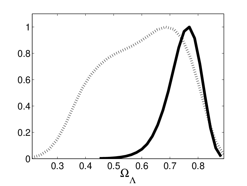


Finally, we look at the CDM + model where we look for better constraints on dark energy equation of state (). The constraint on is modestly improved, since the dark energy equation of state changes the growth factor along the WMAP degeneracy curve, thus the evolution of the gravitational potential. We also see that there is a tilt of towards lower value when we combine WMAP with ISW and WL effects. We also plot the 2-D contours for the and in Fig 18.
As mentioned above, WMAP 3-year model predicts ISW amplitude that is about two sigma below our constraints and this is also the case for the best fit CDM model (which is almost the same as WMAP 3-year). Adding curvature or dark energy equation of state does not reduce this discrepancy either and in both cases these two parameters are not needed to improve the fit. While reducing matter density goes in the desired direction of increasing ISW in cross-correlations, such models also increase the CMB power at large scales through the ISW auto-correlation power, which is in disagreement with the low power observed on large scales in WMAP. For example, we find that there are models with which improve the fit to ISW data by 13 relative to the best fit CDM + model, but at the same time make the WMAP fit worse by 15. There is thus some mild tension between low power in WMAP at low and the high ISW power we measure, but it is a tension that cannot be removed by simple extensions of parameter space explored here. As this is only a two sigma effect there is a considerable probability that it is just a statistical fluctuation.
| Parameter | Limits (CMB+ISW+WL) | Limits (CMB+ISW) |
|---|---|---|

| Parameter | C() | C() | C() | C() | C() | I() | I() | I() | I() | I() | |
|---|---|---|---|---|---|---|---|---|---|---|---|
| CDM, 6 parameters | |||||||||||
| 0.0208 | 0.0214 | 0.0222 | 0.0229 | 0.0236 | 0.0208 | 0.0215 | 0.0222 | 0.0229 | 0.0236 | ||
| 0.0901 | 0.0976 | 0.105 | 0.113 | 0.121 | 0.0901 | 0.0970 | 0.104 | 0.111 | 0.119 | ||
| 0.0312 | 0.0612 | 0.0911 | 0.121 | 0.151 | 0.0359 | 0.0662 | 0.0956 | 0.125 | 0.154 | ||
| 0.929 | 0.943 | 0.959 | 0.976 | 0.993 | 0.929 | 0.944 | 0.960 | 0.977 | 0.994 | ||
| 0.684 | 0.724 | 0.760 | 0.793 | 0.822 | 0.698 | 0.734 | 0.766 | 0.796 | 0.822 | ||
| 0.178 | 0.207 | 0.240 | 0.276 | 0.316 | 0.178 | 0.204 | 0.234 | 0.266 | 0.302 | ||
| 0.670 | 0.717 | 0.767 | 0.816 | 0.863 | 0.671 | 0.715 | 0.763 | 0.810 | 0.855 | ||
| 67.0 | 69.9 | 72.9 | 76.3 | 79.7 | 67.9 | 70.6 | 73.5 | 76.6 | 79.8 | ||
| CDM + , 7 parameters | |||||||||||
| 0.0203 | 0.0211 | 0.0218 | 0.0226 | 0.0233 | 0.0206 | 0.0213 | 0.0221 | 0.0229 | 0.0236 | ||
| 0.0916 | 0.0990 | 0.107 | 0.115 | 0.123 | 0.0900 | 0.0968 | 0.104 | 0.112 | 0.120 | ||
| 0.0269 | 0.0546 | 0.0836 | 0.113 | 0.142 | 0.0330 | 0.0637 | 0.0934 | 0.123 | 0.152 | ||
| -0.147 | -0.115 | -0.0499 | -0.00574 | 0.0150 | -0.0515 | -0.0235 | -0.00395 | 0.0103 | 0.0201 | ||
| 0.917 | 0.932 | 0.948 | 0.966 | 0.984 | 0.925 | 0.941 | 0.958 | 0.976 | 0.993 | ||
| 0.332 | 0.437 | 0.606 | 0.745 | 0.821 | 0.610 | 0.691 | 0.754 | 0.802 | 0.837 | ||
| 0.166 | 0.262 | 0.445 | 0.678 | 0.804 | 0.148 | 0.190 | 0.250 | 0.330 | 0.436 | ||
| 0.648 | 0.690 | 0.738 | 0.788 | 0.839 | 0.663 | 0.709 | 0.758 | 0.807 | 0.857 | ||
| 40.5 | 43.6 | 53.8 | 69.5 | 86.6 | 54.0 | 62.1 | 71.0 | 81.3 | 92.0 | ||
| CDM + , 7 parameters | |||||||||||
| 0.0208 | 0.0215 | 0.0222 | 0.0231 | 0.0239 | 0.0207 | 0.0214 | 0.0222 | 0.0230 | 0.237 | ||
| 0.0900 | 0.0981 | 0.106 | 0.114 | 0.122 | 0.0906 | 0.0975 | 0.105 | 0.112 | 0.120 | ||
| 0.0294 | 0.0600 | 0.0894 | 0.119 | 0.149 | 0.0347 | 0.0647 | 0.0940 | 0.123 | 0.153 | ||
| -1.731 | -1.457 | -1.031 | -0.573 | -0.240 | -1.646 | -1.401 | -1.006 | -0.704 | -0.425 | ||
| 0.927 | 0.943 | 0.960 | 0.981 | 1.010 | 0.928 | 0.943 | 0.960 | 0.978 | 0.998 | ||
| 0.457 | 0.617 | 0.764 | 0.844 | 0.870 | 0.546 | 0.672 | 0.778 | 0.845 | 0.871 | ||
| 0.130 | 0.156 | 0.235 | 0.383 | 0.543 | 0.128 | 0.155 | 0.220 | 0.328 | 0.454 | ||
| 0.437 | 0.613 | 0.776 | 0.919 | 1.032 | 0.540 | 0.659 | 0.781 | 0.898 | 1.00 | ||
| 47.8 | 57.9 | 73.8 | 90.7 | 98.5 | 53.2 | 62.4 | 75.6 | 90.2 | 98.2 | ||
VIII Discussion
The main goal of this paper is to perform a full analysis of the integrated Sachs-Wolfe effect using the cross-correlations between WMAP CMB maps and maps of large scale structure. In contrast to previous work on this subject we place less emphasis on establishing a detection of ISW and more emphasis on developing a tool with which cosmological models can be compared to the data in a close to optimal fashion. For this reason we only select the data sets that can be reliably used towards this goal, as discussed in more detail below. The redshift range of the datasets we use is between 0 and 2.5. We use optimal weighting of the data both in angular space and in redshift space to extract the maximum amount of information, taking into account properly the correlations between them. Our final product is the likelihood function with which different cosmological models can be compared to each other.
As the ISW effect is both a probe of cosmological parameters and a consistency test of the standard CDM cosmology, there have been significant previous efforts made to detect it. A number of different analysis methods have been used and the WMAP data have been cross-correlated with several samples. These include the 2MASS XSC; several SDSS samples including magnitude-limited galaxy samples, LRGs, and quasars; the NVSS; and the HEAO hard X-ray map. Most of these samples (or samples with similar spatial coverage and redshift range) are included in the present work, but not all. Here we compare our analysis with the previous work and comment on the reasons for our choice of data sets.
- 1.
Near-infrared galaxies (2MASS). The 2MASS galaxies are useful for ISW due to high sky coverage and the ability to see closer to the Galactic plane in the near-IR than in the optical. However they can only probe the lowest redshifts (). Afshordi et al. [14] and Rassat et al. [25] have measured the ISW signal using the 2MASS sample and we deliberately cut our 2MASS sample into brightness bins such as theirs so that we can compare the results. We find that our measured signal from 2MASS is very similar. We do however derive cosmological constraints using a Markov chain (which fits all the cosmological parameters instead of just ) from these samples. We also take into account (albeit in a crude way) the redshift dependence of the bias resulting from seeing all nearby galaxies but only the brightest and most biased galaxies at .
- 2.
Optical galaxies (SDSS, APM). Wide-angle multicolor galaxy surveys such as SDSS open almost limitless possibilities for constructing galaxy samples, and many of these samples have been used in previous ISW work. Most work so far has been on either flux-limited samples [12, 20], which have a broad redshift distribution, or photometric LRGs [12, 13, 18, 20], which can be seen to larger distances and for which it is easier to construct reliable photo- cuts. In SDSS, photometric LRG samples oversample the linear density field in the redshift range and the lower redshifts are covered by 2MASS, so the flux-limited galaxy samples would be redundant in terms of volume for our study; we therefore did not include them. Our LRG samples cover the largest solid angle to date of any SDSS ISW analysis (6641 deg2) and for the purposes of cosmological analysis are split into two photo- slices. Fosalba & Gaztañaga [16] have also used galaxies from the Automated Plate Measuring (APM) survey [89], which adds deg2 in the Southern Hemisphere inaccessible to SDSS. Their APM sample has a typical redshift and thus would add some information beyond the most distant of our 2MASS samples. Considering that APM area is only 16% of 2MASS and that it only marginally extends the redshift range we have not used APM in our analysis. However adding a deeper galaxy survey in the South, comparable to or deeper than SDSS, would be valuable for improving ISW constraints. Overall signal to noise from SDSS LRG galaxies is about 3, most of which comes from the higher redshift sample around .
- 3.
Optical quasars (SDSS). Photometrically selected quasars can probe large-scale structure at much higher redshifts than “normal” galaxies because they are bright enough to be seen in wide-angle surveys (such as SDSS) even at . The only ISW analysis with quasars so far has been that of Giannantonio et al. [21], who cross-correlated WMAP with a sample of photometric quasars from the SDSS. Our analysis uses similar selection criteria, but we have used photo- cuts to eliminate most of the lower-redshift objects, and used a combination of spectroscopic data and angular clustering to constrain taking into account the multimodal nature of the photo- failures. We also slice our quasars into two photo- bins. Despite these improvements we find that the significance is only 1.3 (1.24 for the high redshift sample with ), and we therefore do not confirm that the 2.1 signal seen in [21] comes from .
- 4.
Radio sources (NVSS). There have been several past WMAPNVSS ISW analyses [15, 17, 23, 24], taking advantage of the high redshift (compared to most optical samples) and wide sky coverage of the NVSS. We have used the angular power spectrum whereas the previous works have used correlation functions or wavelet coefficients. However, the most important difference between our analysis and the previous result is that we fit from cross-correlations rather than using the Dunlop & Peacock model [77] for the redshift distribution and assuming constant bias. This is important as we find the fit looks very different (see Fig. 13). All of these studies, including ours, have found positive cross correlations at the level. However, the interpretation of this result depends sensitively on one’s ability to measure and this is where we believe our analysis is an improvement upon previous efforts.
- 5.
Hard X-ray background (HEAO). Boughn & Crittenden [15] have used the HEAO hard X-ray map [90] for ISW cross-correlation. The background is due mainly to unresolved (by HEAO) active galactic nuclei and hence traces large scale structure at redshifts of order unity. This, combined with the all-sky nature of HEAO, is beneficial for ISW projects. However, we decided not to add in HEAO sample to our analysis for several reasons. First is the difficulty in understanding the of the sample (we use the general notation here even though for unresolved X-ray flux it would be more accurate to write ). Only % of the background is resolved by Chandra into sources with measured redshifts [91, 92], and we have little guidance on where to place the other 25%. Even if we knew perfectly, this does not tell us : the modeled spans the range and it is unlikely that the bias would be even approximately constant over this range. An alternative is to fit for their bias and redshift distributions up to high using a cross-correlation method similar to that done for NVSS in Sec. V. Unfortunately HEAO has FWHM of and does not resolve individual sources, so we would have to fit the data to the model without small-scale information, which loses signal-to-noise on the cross-correlation very rapidly. A secondary reason is that there is considerable overlap between HEAO and NVSS, so it is likely that the two trace partly the same structure, and thus the improvement in ISW constraint is not as large as adding two independent data sets. We note that it may make sense to include the hard X-ray maps in parameter estimation in the future if a robust determination of becomes available.
In summary, we believe we used most of the available large scale structure data useful for ISW analysis. This not only updates previous work on ISW effect [11, 12, 13, 14, 15, 16, 17, 18, 19, 20, 21, 22, 23, 24, 25], but is also the first one that attempts to do the tomography of ISW, in the sense of encompassing a wide redshift range via our mass tracers going from the local Universe to , while reducing the amount of overlap in area and redshift as much as possible. We have argued that many of the previous measurements have a considerable overlap in redshift and area, which means that they cannot be combined independently and that the effective redshift of the sample is not necessarily the redshift from where most of the ISW signal is coming from. Our analysis, while attempting to minimize the overlap in the first place, takes the residual correlations into account explicitly via the construction of the full covariance matrix. We note that Giannantonio et al. 11 1 T. Giannantonio et al., in preparation. are also pursuing an ISW tomography analysis, with somewhat different choices of LSS samples and cross-correlation methodologies.
We spend a significant fraction of our analysis obtaining the correct redshift distributions for all of the samples. To be more accurate, it is the that we constrain for all samples. The signature of ISW effect is highly affected by the redshift distribution of the tracer, and thus one would need to have an accurate idea of what the redshift distribution is in order to interpret the correlation. Apart from employing spectroscopic datasets that overlap in magnitude range and sky coverage, we correlate the tracer samples with one another so as to obtain the for some of the samples. This is mainly possible because LRGs have relatively good photometric redshifts and so we correlate the LRGs with other overlapping datasets to determine what are the at the redshift range that LRGs cover. In addition, we account for redshift-dependent bias in 2MASS and for the multimodal error distributions for the quasars. We also made the first determination of for NVSS sample which is not based simply on a theoretical model fitting the luminosity function.
Correlations of mass tracers with the CMB sky can be caused not only by the ISW effect, but also by other cosmological effect such as thermal SZ, Galactic foregrounds and extinction, and extragalactic point sources. We provide an estimate for all these effects and only include the scales deemed reliable, where the contamination is subdominant or negligible.
We report a detection of of the ISW effect combining 2MASS, SDSS, and NVSS with WMAP data. We make a joint analysis of all samples by constructing a reliable covariance matrix including cross-correlations of different samples, which is needed for cosmological parameter fitting. We combine our ISW correlation functions with weak lensing of the CMB (Paper II) to derive cosmological constraints on three different cosmological models: (i) the “vanilla” CDM model, (ii) CDM+, and (iii) CDM+. We find a slight improvement of our measurement of in model (iii) over the measurement made by CMB alone: instead of . The constraining power of our analysis is however most prominent in determining that curvature of the Universe: for CMB+ISW+WL we find instead of for CMB alone. These constraints are not as tight as that obtained by some other methods, such as combining the CMB with baryonic oscillations or with supernovae [93, 94, 68], but it is subject to very different systematics. It is thus reassuring that all of them are consistent with each other. Even more importantly, there are other models where ISW can be crucial in distinguishing them from standard CDM, such as models in which the growth of structure is not fixed by the background geometry [26]. Some of these models may already be inconsistent with our ISW signal; we plan to present such constraints in a future paper. These constraints should improve further in the future with deeper galaxy surveys that should reach the cosmic variance limit out to , and future CMB data that enables lower-noise lensing reconstruction.
Finally, we would like to note that we plan to release a package for calculating ISW likelihood function given the datasets and cosmological parameters. This will be described further in the documentation for the package.
Acknowledgements.
We would like to thank Joanna Dunkley for her extensive help on the discussion of chain convergences, and Lucas Lombriser and Anže Slosar for bringing an error in an earlier version of this paper to our attention. We would also like to thank David Spergel, Kendrick Smith and Jim Gunn for helpful conversations. C.H. was a John Bahcall fellow at the Institute for Advanced Study during most of the preparation of this paper. N.P. is supported by a Hubble Fellowship HST.HF-01200.01 awarded by the Space Telescope Science Institute, which is operated by the Association of Universities for Research in Astronomy, Inc., for NASA, under contract NAS 5-26555. Part of this work was supported by the Director, Office of Science, of the U.S. Department of Energy under Contract No. DE-AC02-05CH11231. U.S. is supported by the Packard Foundation and NSF CAREER-0132953. Funding for the SDSS and SDSS-II has been provided by the Alfred P. Sloan Foundation, the Participating Institutions, the National Science Foundation, the U.S. Department of Energy, the National Aeronautics and Space Administration, the Japanese Monbukagakusho, the Max Planck Society, and the Higher Education Funding Council for England. The SDSS Web Site is http://www.sdss.org/. The SDSS is managed by the Astrophysical Research Consortium for the Participating Institutions. The Participating Institutions are the American Museum of Natural History, Astrophysical Institute Potsdam, University of Basel, University of Cambridge, Case Western Reserve University, University of Chicago, Drexel University, Fermilab, the Institute for Advanced Study, the Japan Participation Group, Johns Hopkins University, the Joint Institute for Nuclear Astrophysics, the Kavli Institute for Particle Astrophysics and Cosmology, the Korean Scientist Group, the Chinese Academy of Sciences (LAMOST), Los Alamos National Laboratory, the Max-Planck-Institute for Astronomy (MPIA), the Max-Planck-Institute for Astrophysics (MPA), New Mexico State University, Ohio State University, University of Pittsburgh, University of Portsmouth, Princeton University, the United States Naval Observatory, and the University of Washington. The 2dF QSO Redshift Survey (2QZ) was compiled by the 2QZ survey team from observations made with the 2-degree Field on the Anglo-Australian Telescope. The 2dF-SDSS LRG and QSO (2SLAQ) Survey was compiled by the 2SLAQ team from SDSS data and observations made with the 2-degree Field on the Anglo-Australian Telescope. This publication makes use of data products from the Two Micron All Sky Survey, which is a joint project of the University of Massachusetts and the Infrared Processing and Analysis Center/California Institute of Technology, funded by the National Aeronautics and Space Administration and the National Science Foundation.Appendix A NVSS redshift window functions
In Sec. V.4.3, we fit a constant to the cross-spectra of NVSS and the other LSS samples. We argued that this procedure gave an estimator whose expectation value was given by Eq. (34). The purpose of this appendix is to prove this equation and construct the functional form .
We begin by noting that we have measured cross-spectra and their covariance matrix . The theoretical cross-spectrum is on the other hand simply the Limber result,
| (49) | |||||
where is the comoving angular diameter distance and is defined by the equivalence in the second line. The fitting procedure for the constant is to minimize
| (50) | |||||
where and are the measured cross-spectra. The minimum value of is obtained for
| (51) |
Since the have expectation value given by Eq. (49), we have
| (52) |
This proves Eq. (34) and shows that the window function is
| (53) |
Appendix B Error bars on galaxy-CMB correlations
The purpose of this appendix is to discuss our choice of the Monte Carlo (“MC1”) estimator for the error bars on the estimator, and then give a crude estimate for the possible biases that are induced by its use. As mentioned in the main text there are two biases: the correlation bias (because the galaxies and CMB are correlated and MC1 does not take this into account) and a realization bias (since we have only one realization of the galaxies). The correlation bias is deterministic in the sense that the error bar is always underestimated in every -bin. The realization bias is more subtle: if , then the MC1 estimator returns an unbiased estimate of . However the -bins where the error is underestimated are weighted more heavily than those where it is overestimated, resulting in a final error bar on cosmological parameters that is biased low.
We consider each of these issues separately in a toy model. The toy model has the following assumptions:
- 1.
We are computing cross-spectra in -bins (call these cross-spectra ).
- 2.
The galaxies and CMB temperature are Gaussian random fields. (We are at linear scales where large scale structure is Gaussian; the systematics may not be.)
- 3.
In the th -bin, there are galaxy modes, and all of the CMB modes in this region are observed. (This is true except that NVSS goes slightly closer to the Galactic plane than WMAP.) We ignore mode coupling at the boundaries, i.e. each mode is ascribed to a single -bin.
- 4.
We are fitting the cross-correlation data to some parameter, say an amplitude of some template . More generally, when the ISW effect is essentially constraining one direction in parameter space with all others constrained by the CMB alone (the case with CDM+ and CDM+ models here) the template would be where parameterizes the CMB-degenerate direction. The fit is done using the Monte Carlo covariance matrix.
- 5.
The objective is to determine what is the ratio of the “true” error bar on to that derived from the fitting procedure.
Within these assumptions, we evaluate the correlation bias and realization bias , which we define to be the ratio of true to estimated variance. We find, using correlation coefficients and numbers of modes for the worst-case bins, that and . This corresponds to % underestimation of the error bars in the worst case, which is negligible.
B.1 Correlation bias
We will introduce the notation for the galaxy power spectrum including Poisson noise, and for a matrix Cov we will write Cov to mean the element of Cov-1 rather than the reciprocal of Covij. (In the cases considered in this appendix the covariance matrices are diagonal so this distinction will not matter.) We will also use the shorthand for the galaxy-temperature cross-spectrum in the th bin.
The estimator for the cross correlation is
| (54) |
where is a mode index.
The true uncertainty in Gaussian theory, using independence of modes, is
| (55) |
However the MC1 procedure gives
| (56) |
where the modes are in bin , the beta modes are in bin , and is the actual realization of the galaxies. Simplifying with CMB covariance matrix gives
| (57) |
Note that this is diagonal, even though we have only Monte-Carloed one of the data sets.
In the presence of a nonzero cross-correlation, the MC1 covariance matrix is biased:
| (58) |
where the correlation coefficient is
| (59) |
For the fiducial cosmology and the bins that we used, the maximum predicted correlation coefficient is 0.067 (LRG1, ). This would suggest an underestimate of the error bar by a factor of . For some cosmological models, such as those with lower or higher , the correlation coefficient could be larger. Indeed there is some evidence for this: we observe an overall ISW amplitude of times the prediction. If we multiply the correlation coefficient by 2.2 then the underestimate of the error bar grows to ; even this is negligible.
B.2 Realization bias
Having taken into account the correlation bias, we now consider the case where the cross-correlation coefficient is small (). In this case, the covariance matrix of the that we obtain from the CMB Monte Carlos is unbiased. The realization bias comes from the fact that we invert the covariance matrix, and unbiased Cov does not imply unbiased Cov.
The true covariance matrix of the estimator Eq. (54) for is
| (60) |
where and are the true (ensemble-averaged) galaxy and CMB power spectra, including Poisson noise for the galaxies. The estimated covariance matrix is instead given by Eq. (57). Now define the number
| (61) |
which is the ratio of the estimated to true variance in a given bin. This simplifies to
| (62) |
i.e. it is a distribution with degrees of freedom, divided by the number of degrees of freedom. In particular : the covariance matrix is unbiased, but we have from distribution theory and .
However what we really want to compare are the true and estimated errors on the parameter . The estimate of the amplitude is
| (63) |
Its estimated variance is
| (64) |
Its true variance is
| (65) |
(Note that and are uncorrelated because the probability distribution is symmetric in , under which changes sign but does not.) The ratio is
| (66) |
Using the definition of and diagonality of the matrices Cov and ,
| (67) |
We now consider two limiting cases. If we have a single -bin, then the ratio is and
| (68) |
If we have many -bins contributing then the sums go to their mean values and we get
| (69) |
if there were the same number of modes in each -bin. This is larger than Eq. (68) because with only a single bin there is then no possibility for the amplitude estimator to re-weight the bins to take advantage of the ones with smaller estimated variance.
The number of modes per bin is, in the limit of negligible mode coupling,
| (70) |
This is 40 for the lowest- 2MASS bin that we use in parameter fits, 77 for the lowest- LRGs, 70 for the quasars, and 40 for NVSS. To be pessimistic, if we take Eq. (69) for all these cases the worst number we get is , which means that in this pessimistic case we have underestimated the error bar () on the cross-correlation by 5%. In reality much of the constraint comes from higher- bins where is greater, so this should be taken as an upper limit.
Appendix C Signal to noise estimate and upper limit on foreground contamination
To assess the statistical signal to noise we look at correlation between the galaxy overdensity and the temperature of the CMB (), which is the data vector called . We also need its inverse covariance matrix () and the theoretical prediction, which we can model as amplitude times a fiducial model . To assess the possible contamination from foregrounds, tSZ, point sources etc. to our signal we need to estimate the associated cross-correlation contamination . For example, for foregrounds we look at the correlation between the galaxy overdensity and the foreground temperature (which is what we calculated using models such as described by Eq. 44).
Consider the usual analysis, where we are trying to fit for given , and :
| (71) |
We minimize and get
| (72) |
This is Eq. (45) and the associated variance is given by Eq. (46). The ratio of estimated amplitude to its variance is the estimated signal to noise.
Since the total signal is a sum of the true signal and contamination such as foreground, tSZ or point sources, the latter contribute to the signal to noise,
| (73) |
While we could use this expression to estimate the possible contamination we can make it less dependent on the weighting by theoretical model by using the Cauchy inequality, here written in the (primed) diagonal basis with eigenvectors normalized to eigenvalue, , to derive from Eq. (73):
| (74) |
We use this expression in our estimates of contamination; it represents an upper limit on the number of sigmas of contamination introduced by the foreground .
References
- [1] C. M. Hirata, S. Ho, N. Padmanabhan, U. Seljak, and N. A. Bahcall (2008), eprint arXiv:0801.0644.
- [2] G. F. Smoot, C. L. Bennett, A. Kogut, E. L. Wright, J. Aymon, N. W. Boggess, E. S. Cheng, G. de Amici, S. Gulkis, M. G. Hauser, et al., Astrophys. J Lett. 396, L1 (1992).
- [3] C. L. Bennett, R. S. Hill, G. Hinshaw, M. R. Nolta, N. Odegard, L. Page, D. N. Spergel, J. L. Weiland, E. L. Wright, M. Halpern, et al., Astrophys. J Supp. 148, 97 (2003), eprint arXiv:astro-ph/0302208.
- [4] N. Jarosik, C. Barnes, M. R. Greason, R. S. Hill, M. R. Nolta, N. Odegard, J. L. Weiland, R. Bean, C. L. Bennett, O. Doré, et al., Astrophys. J Supp. 170, 263 (2007), eprint arXiv:astro-ph/0603452.
- [5] M. Tegmark, D. J. Eisenstein, M. A. Strauss, D. H. Weinberg, M. R. Blanton, J. A. Frieman, M. Fukugita, J. E. Gunn, A. J. S. Hamilton, G. R. Knapp, et al., Phys. Rev. D 74, 123507 (2006), eprint arXiv:astro-ph/0608632.
- [6] W. L. Freedman, S. M. Hughes, B. F. Madore, J. R. Mould, M. G. Lee, P. Stetson, R. C. Kennicutt, A. Turner, L. Ferrarese, H. Ford, et al., Astrophys. J. 427, 628 (1994).
- [7] S. Cole, W. J. Percival, J. A. Peacock, P. Norberg, C. M. Baugh, C. S. Frenk, I. Baldry, J. Bland-Hawthorn, T. Bridges, R. Cannon, et al., Mon. Not. R. Astron. Soc. 362, 505 (2005), eprint arXiv:astro-ph/0501174.
- [8] R. A. Sunyaev and I. B. Zeldovich, Mon. Not. R. Astron. Soc. 190, 413 (1980a).
- [9] R. A. Sunyaev and I. B. Zeldovich, Ann. Rev. Astron. Astrophys. 18, 537 (1980b).
- [10] R. K. Sachs and A. M. Wolfe, Astrophys. J. 147, 73 (1967).
- [11] S. P. Boughn, R. G. Crittenden, and N. G. Turok, New Astronomy 3, 275 (1998), eprint arXiv:astro-ph/9704043.
- [12] P. Fosalba, E. Gaztañaga, and F. J. Castander, Astrophys. J Lett. 597, L89 (2003), eprint arXiv:astro-ph/0307249.
- [13] R. Scranton, A. J. Connolly, R. C. Nichol, A. Stebbins, I. Szapudi, D. J. Eisenstein, N. Afshordi, T. Budavari, I. Csabai, J. A. Frieman, et al., ArXiv Astrophysics e-prints (2003), eprint astro-ph/0307335.
- [14] N. Afshordi, Y.-S. Loh, and M. A. Strauss, Phys. Rev. D 69, 083524 (2004), eprint arXiv:astro-ph/0308260.
- [15] S. Boughn and R. Crittenden, Nature (London) 427, 45 (2004a), eprint arXiv:astro-ph/0305001.
- [16] P. Fosalba and E. Gaztañaga, Monthly Notices of the Royal Astronomical Society 350, L37 (2004).
- [17] M. R. Nolta, E. L. Wright, L. Page, C. L. Bennett, M. Halpern, G. Hinshaw, N. Jarosik, A. Kogut, M. Limon, S. S. Meyer, et al., Astrophys. J. 608, 10 (2004), eprint arXiv:astro-ph/0305097.
- [18] N. Padmanabhan, C. M. Hirata, U. Seljak, D. J. Schlegel, J. Brinkmann, and D. P. Schneider, Phys. Rev. D 72, 043525 (2005a), eprint arXiv:astro-ph/0410360.
- [19] E. Gaztañaga, M. Manera, and T. Multamäki, Mon. Not. R. Astron. Soc. 365, 171 (2006), eprint arXiv:astro-ph/0407022.
- [20] A. Cabré, E. Gaztañaga, M. Manera, P. Fosalba, and F. Castander, Mon. Not. R. Astron. Soc. 372, L23 (2006), eprint arXiv:astro-ph/0603690.
- [21] T. Giannantonio, R. G. Crittenden, R. C. Nichol, R. Scranton, G. T. Richards, A. D. Myers, R. J. Brunner, A. G. Gray, A. J. Connolly, and D. P. Schneider, Phys. Rev. D 74, 063520 (2006), eprint arXiv:astro-ph/0607572.
- [22] P. Vielva, E. Martínez-González, and M. Tucci, Mon. Not. R. Astron. Soc. 365, 891 (2006), eprint arXiv:astro-ph/0408252.
- [23] D. Pietrobon, A. Balbi, and D. Marinucci, Phys. Rev. D 74, 043524 (2006), eprint arXiv:astro-ph/0606475.
- [24] J. D. McEwen, P. Vielva, M. P. Hobson, E. Martínez-González, and A. N. Lasenby, Mon. Not. R. Astron. Soc. 376, 1211 (2007), eprint arXiv:astro-ph/0602398.
- [25] A. Rassat, K. Land, O. Lahav, and F. B. Abdalla, Mon. Not. R. Astron. Soc. 377, 1085 (2007).
- [26] Y.-S. Song, H. Peiris, and W. Hu, Phys. Rev. D 76, 063517 (2007), eprint arXiv:0706.2399.
- [27] H. V. Peiris and D. N. Spergel, Astrophys. J. 540, 605 (2000), eprint arXiv:astro-ph/0001393.
- [28] A. Cooray, Phys. Rev. D 65, 103510 (2002), eprint arXiv:astro-ph/0112408.
- [29] K. M. Górski, E. Hivon, A. J. Banday, B. D. Wandelt, F. K. Hansen, M. Reinecke, and M. Bartelmann, Astrophys. J. 622, 759 (2005), eprint arXiv:astro-ph/0409513.
- [30] T. H. Jarrett, T. Chester, R. Cutri, S. Schneider, M. Skrutskie, and J. P. Huchra, Astron. J. 119, 2498 (2000), eprint arXiv:astro-ph/0004318.
- [31] M. F. Skrutskie, S. E. Schneider, R. Stiening, S. E. Strom, M. D. Weinberg, C. Beichman, T. Chester, R. Cutri, C. Lonsdale, J. Elias, et al., in Astrophysics and Space Science Library, edited by F. Garzon, N. Epchtein, A. Omont, B. Burton, and P. Persi (1997), vol. 210 of Astrophysics and Space Science Library, pp. 25–+.
- [32] M. F. Skrutskie, R. M. Cutri, R. Stiening, M. D. Weinberg, S. Schneider, J. M. Carpenter, C. Beichman, R. Capps, T. Chester, J. Elias, et al., Astron. J. 131, 1163 (2006).
- [33] D. J. Schlegel, D. P. Finkbeiner, and M. Davis, Astrophys. J. 500, 525 (1998), eprint arXiv:astro-ph/9710327.
- [34] D. G. York, J. Adelman, J. E. Anderson, Jr., S. F. Anderson, J. Annis, N. A. Bahcall, J. A. Bakken, R. Barkhouser, S. Bastian, E. Berman, et al., Astron. J. 120, 1579 (2000), eprint arXiv:astro-ph/0006396.
- [35] J. E. Gunn, M. Carr, C. Rockosi, M. Sekiguchi, K. Berry, B. Elms, E. de Haas, Ž. Ivezić, G. Knapp, R. Lupton, et al., Astron. J. 116, 3040 (1998), eprint arXiv:astro-ph/9809085.
- [36] J. E. Gunn, W. A. Siegmund, E. J. Mannery, R. E. Owen, C. L. Hull, R. F. Leger, L. N. Carey, G. R. Knapp, D. G. York, W. N. Boroski, et al., Astron. J. 131, 2332 (2006), eprint arXiv:astro-ph/0602326.
- [37] D. W. Hogg, D. P. Finkbeiner, D. J. Schlegel, and J. E. Gunn, Astron. J. 122, 2129 (2001), eprint arXiv:astro-ph/0106511.
- [38] M. Fukugita, T. Ichikawa, J. E. Gunn, M. Doi, K. Shimasaku, and D. P. Schneider, Astron. J. 111, 1748 (1996).
- [39] J. A. Smith, D. L. Tucker, S. Kent, M. W. Richmond, M. Fukugita, T. Ichikawa, S.-i. Ichikawa, A. M. Jorgensen, A. Uomoto, J. E. Gunn, et al., Astron. J. 123, 2121 (2002), eprint arXiv:astro-ph/0201143.
- [40] R. Lupton, J. E. Gunn, Z. Ivezić, G. R. Knapp, and S. Kent, in Astronomical Data Analysis Software and Systems X, edited by F. R. Harnden, Jr., F. A. Primini, and H. E. Payne (2001), vol. 238 of Astronomical Society of the Pacific Conference Series, pp. 269–+.
- [41] J. R. Pier, J. A. Munn, R. B. Hindsley, G. S. Hennessy, S. M. Kent, R. H. Lupton, and Ž. Ivezić, Astron. J. 125, 1559 (2003), eprint arXiv:astro-ph/0211375.
- [42] D. L. Tucker, S. Kent, M. W. Richmond, J. Annis, J. A. Smith, S. S. Allam, C. T. Rodgers, J. L. Stute, J. K. Adelman-McCarthy, J. Brinkmann, et al., Astronomische Nachrichten 327, 821 (2006), eprint arXiv:astro-ph/0608575.
- [43] N. Padmanabhan, D. J. Schlegel, D. P. Finkbeiner, J. C. Barentine, M. R. Blanton, H. J. Brewington, J. E. Gunn, M. Harvanek, D. W. Hogg, Z. Ivezic, et al., ArXiv Astrophysics e-prints (2007a), eprint astro-ph/0703454.
- [44] D. J. Eisenstein, J. Annis, J. E. Gunn, A. S. Szalay, A. J. Connolly, R. C. Nichol, N. A. Bahcall, M. Bernardi, S. Burles, F. J. Castander, et al., Astron. J. 122, 2267 (2001), eprint arXiv:astro-ph/0108153.
- [45] M. A. Strauss, D. H. Weinberg, R. H. Lupton, V. K. Narayanan, J. Annis, M. Bernardi, M. Blanton, S. Burles, A. J. Connolly, J. Dalcanton, et al., Astron. J. 124, 1810 (2002), eprint arXiv:astro-ph/0206225.
- [46] G. T. Richards, X. Fan, H. J. Newberg, M. A. Strauss, D. E. Vanden Berk, D. P. Schneider, B. Yanny, A. Boucher, S. Burles, J. A. Frieman, et al., Astron. J. 123, 2945 (2002), eprint arXiv:astro-ph/0202251.
- [47] M. R. Blanton, H. Lin, R. H. Lupton, F. M. Maley, N. Young, I. Zehavi, and J. Loveday, Astron. J. 125, 2276 (2003), eprint arXiv:astro-ph/0105535.
- [48] C. Stoughton, R. H. Lupton, M. Bernardi, M. R. Blanton, S. Burles, F. J. Castander, A. J. Connolly, D. J. Eisenstein, J. A. Frieman, G. S. Hennessy, et al., Astron. J. 123, 485 (2002).
- [49] K. Abazajian, J. K. Adelman-McCarthy, M. A. Agüeros, S. S. Allam, S. F. Anderson, J. Annis, N. A. Bahcall, I. K. Baldry, S. Bastian, A. Berlind, et al., Astron. J. 126, 2081 (2003).
- [50] K. Abazajian, J. K. Adelman-McCarthy, M. A. Agüeros, S. S. Allam, K. Anderson, S. F. Anderson, J. Annis, N. A. Bahcall, I. K. Baldry, S. Bastian, et al., Astron. J. 128, 502 (2004), eprint arXiv:astro-ph/0403325.
- [51] K. Abazajian, J. K. Adelman-McCarthy, M. A. Agüeros, S. S. Allam, K. S. J. Anderson, S. F. Anderson, J. Annis, N. A. Bahcall, I. K. Baldry, S. Bastian, et al., Astron. J. 129, 1755 (2005), eprint arXiv:astro-ph/0410239.
- [52] J. K. Adelman-McCarthy, M. A. Agüeros, S. S. Allam, K. S. J. Anderson, S. F. Anderson, J. Annis, N. A. Bahcall, I. K. Baldry, J. C. Barentine, A. Berlind, et al., Astrophys. J Supp. 162, 38 (2006), eprint arXiv:astro-ph/0507711.
- [53] J. K. Adelman-McCarthy, M. A. Agüeros, S. S. Allam, K. S. J. Anderson, S. F. Anderson, J. Annis, N. A. Bahcall, C. A. L. Bailer-Jones, I. K. Baldry, J. C. Barentine, et al., Astrophys. J Supp. 172, 634 (2007), eprint arXiv:0707.3380.
- [54] J. K. Adelman-McCarthy and for the SDSS Collaboration, ArXiv e-prints 707 (2007), eprint 0707.3413.
- [55] N. Padmanabhan, T. Budavári, D. J. Schlegel, T. Bridges, J. Brinkmann, R. Cannon, A. J. Connolly, S. M. Croom, I. Csabai, M. Drinkwater, et al., Mon. Not. R. Astron. Soc. 359, 237 (2005b), eprint arXiv:astro-ph/0407594.
- [56] G. T. Richards, R. C. Nichol, A. G. Gray, R. J. Brunner, R. H. Lupton, D. E. Vanden Berk, S. S. Chong, M. A. Weinstein, D. P. Schneider, S. F. Anderson, et al., Astrophys. J Supp. 155, 257 (2004), eprint arXiv:astro-ph/0408505.
- [57] G. T. Richards, M. A. Strauss, X. Fan, P. B. Hall, S. Jester, D. P. Schneider, D. E. Vanden Berk, C. Stoughton, S. F. Anderson, R. J. Brunner, et al., Astron. J. 131, 2766 (2006), eprint arXiv:astro-ph/0601434.
- [58] J. J. Condon, W. D. Cotton, E. W. Greisen, Q. F. Yin, R. A. Perley, G. B. Taylor, and J. J. Broderick, Astron. J. 115, 1693 (1998).
- [59] C. G. T. Haslam, C. J. Salter, and H. Stoffel, in Origin of Cosmic Rays, edited by G. Setti, G. Spada, and A. W. Wolfendale (1981), vol. 94 of IAU Symposium, pp. 217–+.
- [60] C. Blake and J. Wall, Mon. Not. R. Astron. Soc. 329, L37 (2002), eprint arXiv:astro-ph/0111328.
- [61] G. Efstathiou, Mon. Not. R. Astron. Soc. 349, 603 (2004), eprint arXiv:astro-ph/0307515.
- [62] R. E. Smith, J. A. Peacock, A. Jenkins, S. D. M. White, C. S. Frenk, F. R. Pearce, P. A. Thomas, G. Efstathiou, and H. M. P. Couchman, Mon. Not. R. Astron. Soc. 341, 1311 (2003), eprint arXiv:astro-ph/0207664.
- [63] L. Page, C. Barnes, G. Hinshaw, D. N. Spergel, J. L. Weiland, E. Wollack, C. L. Bennett, M. Halpern, N. Jarosik, A. Kogut, et al., Astrophys. J Supp. 148, 39 (2003), eprint arXiv:astro-ph/0302214.
- [64] M. Tegmark, Phys. Rev. D 55, 5895 (1997), eprint arXiv:astro-ph/9611174.
- [65] U. Seljak, Astrophys. J. 506, 64 (1998), eprint arXiv:astro-ph/9711124.
- [66] N. Padmanabhan, U. Seljak, and U. L. Pen, New Astronomy 8, 581 (2003), eprint arXiv:astro-ph/0210478.
- [67] C. M. Hirata, N. Padmanabhan, U. Seljak, D. Schlegel, and J. Brinkmann, Phys. Rev. D 70, 103501 (2004), eprint arXiv:astro-ph/0406004.
- [68] D. N. Spergel, R. Bean, O. Doré, M. R. Nolta, C. L. Bennett, J. Dunkley, G. Hinshaw, N. Jarosik, E. Komatsu, L. Page, et al., Astrophys. J Supp. 170, 377 (2007), eprint arXiv:astro-ph/0603449.
- [69] R. Cannon, M. Drinkwater, A. Edge, D. Eisenstein, R. Nichol, P. Outram, K. Pimbblet, R. de Propris, I. Roseboom, D. Wake, et al., Mon. Not. R. Astron. Soc. 372, 425 (2006), eprint arXiv:astro-ph/0607631.
- [70] N. Padmanabhan, D. J. Schlegel, U. Seljak, A. Makarov, N. A. Bahcall, M. R. Blanton, J. Brinkmann, D. J. Eisenstein, D. P. Finkbeiner, J. E. Gunn, et al., Mon. Not. R. Astron. Soc. 378, 852 (2007b), eprint arXiv:astro-ph/0605302.
- [71] S. M. Croom, R. J. Smith, B. J. Boyle, T. Shanks, L. Miller, P. J. Outram, and N. S. Loaring, Mon. Not. R. Astron. Soc. 349, 1397 (2004), eprint arXiv:astro-ph/0403040.
- [72] G. T. Richards, S. M. Croom, S. F. Anderson, J. Bland-Hawthorn, B. J. Boyle, R. De Propris, M. J. Drinkwater, X. Fan, J. E. Gunn, Ž. Ivezić, et al., Mon. Not. R. Astron. Soc. 360, 839 (2005), eprint arXiv:astro-ph/0504300.
- [73] A. D. Myers, R. J. Brunner, G. T. Richards, R. C. Nichol, D. P. Schneider, D. E. Vanden Berk, R. Scranton, A. G. Gray, and J. Brinkmann, Astrophys. J. 638, 622 (2006), eprint arXiv:astro-ph/0510371.
- [74] S. M. Croom, T. Shanks, B. J. Boyle, R. J. Smith, L. Miller, N. S. Loaring, and F. Hoyle, Mon. Not. R. Astron. Soc. 325, 483 (2001), eprint arXiv:astro-ph/0012375.
- [75] S. M. Croom, B. J. Boyle, T. Shanks, R. J. Smith, L. Miller, P. J. Outram, N. S. Loaring, F. Hoyle, and J. da Ângela, Mon. Not. R. Astron. Soc. 356, 415 (2005), eprint arXiv:astro-ph/0409314.
- [76] Y. Shen, M. A. Strauss, M. Oguri, J. F. Hennawi, X. Fan, G. T. Richards, P. B. Hall, J. E. Gunn, D. P. Schneider, A. S. Szalay, et al., Astron. J. 133, 2222 (2007), eprint arXiv:astro-ph/0702214.
- [77] J. S. Dunlop and J. A. Peacock, Mon. Not. R. Astron. Soc. 247, 19 (1990).
- [78] E. Schinnerer, V. Smolčić, C. L. Carilli, M. Bondi, P. Ciliegi, K. Jahnke, N. Z. Scoville, H. Aussel, F. Bertoldi, A. W. Blain, et al., Astrophys. J Supp. 172, 46 (2007), eprint arXiv:astro-ph/0612314.
- [79] P. Capak, H. Aussel, M. Ajiki, H. J. McCracken, B. Mobasher, N. Scoville, P. Shopbell, Y. Taniguchi, D. Thompson, S. Tribiano, et al., Astrophys. J Supp. 172, 99 (2007), eprint arXiv:0704.2430.
- [80] B. Mobasher, P. Capak, N. Z. Scoville, T. Dahlen, M. Salvato, H. Aussel, D. J. Thompson, R. Feldmann, L. Tasca, O. Lefevre, et al., Astrophys. J Supp. 172, 117 (2007), eprint arXiv:astro-ph/0612344.
- [81] A. Cabre, P. Fosalba, E. Gaztañaga, and M. Manera, Monthly Notices of the Royal Astronomical Society 381, 1347 (2007), eprint arXiv:astro-ph/0701393.
- [82] A. de Oliveira-Costa, M. Tegmark, R. D. Davies, C. M. Gutiérrez, A. N. Lasenby, R. Rebolo, and R. A. Watson, Astrophys. J Lett. 606, L89 (2004), eprint arXiv:astro-ph/0312039.
- [83] D. P. Finkbeiner, Astrophys. J Supp. 146, 407 (2003), eprint arXiv:astro-ph/0301558.
- [84] D. P. Finkbeiner, M. Davis, and D. J. Schlegel, Astrophys. J. 524, 867 (1999), eprint arXiv:astro-ph/9905128.
- [85] Y.-T. Lin and J. J. Mohr, Astrophys. J. 617, 879 (2004), eprint arXiv:astro-ph/0408557.
- [86] S. Ho, Y.-T. Lin, D. Spergel, and C. M. Hirata, ArXiv e-prints 706 (2007), eprint 0706.0727.
- [87] A. Lewis and S. Bridle, Phys. Rev. D 66, 103511 (2002), eprint arXiv:astro-ph/0205436.
- [88] J. Dunkley, M. Bucher, P. G. Ferreira, K. Moodley, and C. Skordis, Mon. Not. R. Astron. Soc. 356, 925 (2005), eprint arXiv:astro-ph/0405462.
- [89] S. J. Maddox, G. Efstathiou, W. J. Sutherland, and J. Loveday, Mon. Not. R. Astron. Soc. 242, 43P (1990).
- [90] E. Boldt, Phys. Rep. 146, 215 (1987).
- [91] L. L. Cowie, A. J. Barger, M. W. Bautz, W. N. Brandt, and G. P. Garmire, Astrophys. J Lett. 584, L57 (2003), eprint arXiv:astro-ph/0301231.
- [92] S. P. Boughn and R. G. Crittenden, Astrophys. J. 612, 647 (2004b), eprint arXiv:astro-ph/0404348.
- [93] D. J. Eisenstein, I. Zehavi, D. W. Hogg, R. Scoccimarro, M. R. Blanton, R. C. Nichol, R. Scranton, H.-J. Seo, M. Tegmark, Z. Zheng, et al., Astrophys. J. 633, 560 (2005), eprint arXiv:astro-ph/0501171.
- [94] U. Seljak, A. Slosar, and P. McDonald, Journal of Cosmology and Astro-Particle Physics 10, 14 (2006), eprint arXiv:astro-ph/0604335.