Single-File Diffusion in a Box

Introduction. - Recent advances in the manufacturing of nanofluidic devices allow studies of geometrically constrained nano - sized particles in quasi one-dimensional systems in which crowding and exclusion effects are important [1, 2]. Situations where large molecules are hindered to overtake also occurs in living systems as, for instance, protein diffusion along DNA [3]. Furthermore, biological cells are characterized by a high degree of molecular crowding [4].

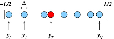
In this Letter, with experiments in mind, akin to [5], we focus on diffusive motion of tagged finite-sized hard-core interacting particles (unable to overtake) (Fig. 1). Such single-file systems show interesting behavior where the $t^{1/2}$ - scaling ($t$ denotes time) of the mean square displacement ${\cal S}(t)=\langle[y_{\cal T}(t)-y_{{\cal T},0}]^{2}\rangle$ in position $y_{\cal T}(t)$ of the tagged particle $[y_{{\cal T},0}\equiv y_{\cal T}(0)]$, for an infinite system with fixed concentration, is most striking ($\langle.\rangle$ denotes ensemble average). Also, the probability density function (PDF) $\rho(y_{\cal T},t|y_{{\cal T},0})\equiv\rho_{\cal T}$ is Gaussian [6, 7, 8]. Even though single-file diffusion has received much attention [9, 10, 11, 8, 12], to our knowledge very few exact results are given for finite-sized particles in finite systems [13]. One exception is [10] where the PDF for $N$ diffusing point particles on a finite interval was obtained. However, asymptotic expressions were only given when the system was made infinite (keeping the concentration finite). Here, we go beyond previous results in the following ways. First, finite-sized particles are considered and we show that the $N$-particle PDF can be written as a Bethe-ansatz solution. Second, we perform a (non-standard) large $N$-analysis of $\rho_{\cal T}$, keeping the system size finite, showing, for the first time, the existence of three dynamical regimes: $(i)$ $t\ll\tau_{\rm coll}=1/\varrho^{2}D$ where $\tau_{\rm coll}$ denotes mean collision time, $D$ the diffusion constant, and $\varrho=N/L$ particle concentration where $L$ is the length of the system, $(ii)$ $\tau_{\rm coll}\ll t\ll\tau_{\rm eq}$ where $\tau_{\rm eq}=L^{2}/D$ is the equilibrium time, and $(iii)$ $t\gg\tau_{\rm eq}$. Notably, only $(i)$ and $(ii)$ are found in infinite systems. Asymptotic expressions for $\rho_{\cal T}$ are derived in regimes $(i)$-$(iii)$ and good agreement with (stochastic) Gillespie simulations [14], is demonstrated.

Statement of the problem. - We study $N$ hard-core interacting particles with linear size $\Delta$ diffusing in a one-dimensional box of length $L$ (Fig. 1). The probability of finding the particles at positions $\vec{y}=(y_{1},\ldots,y_{N})$ at time $t$, given that they initially were at $\vec{y}_{0}=(y_{1,0},\ldots,y_{N,0})$, is contained in the $N$-particle conditional PDF ${\cal P}(\vec{y},t|\vec{y}_{0})$ which is governed by the diffusion equation

Neighboring particles $j$ and $j+1$ are unable to overtake

ensuring that $y_{j+1}-y_{j}\geq\Delta$ $\forall t$ provided that $y_{j,0}<y_{j+1,0}-\Delta$. The boundaries at $\pm L/2$ are reflecting

and the initial PDF is given by

where $\delta(z)$ is the Dirac delta function. The tagged particle PDF studied here is given by [15]

where $\rho_{\rm eq,{\cal T}0}=\int_{{\cal R}_{0}}dy_{1,0}^{\prime}\cdots dy_{N,0}^{\prime}\delta(y_{{\cal T},0}-y_{{\cal T},0}^{\prime}){\cal P}_{\rm eq}(\vec{y}_{0}^{\,{}_{{}^{\prime}}})$, with integration regions ${\cal R}=\{y_{j+1}-y_{j}\geq\Delta,j=1,\ldots,N-1;y_{1}\geq-(L-\Delta)/2;y_{N}\leq(L-\Delta)/2\}$ and ${\cal R}_{0}=\{y_{j+1,0}-y_{j,0}\geq\Delta,j=1,\ldots,N-1;y_{1,0}\geq-(L-\Delta)/2;y_{N,0}\leq(L-\Delta)/2\}$. Initially, the particles are distributed according to the equilibrium density,

$i.e$ the particles are distributed uniformly in the box. The function $\theta(z)$ is the Heaviside step function.

Bethe - ansatz solution. - The (coordinate) Bethe-ansatz yields an integral representation of the PDF in momentum space [11]. The Bethe ansatz satisfying Eqs. (1) - (4) is

where $x_{1},\ldots,x_{N}$ and $x_{1,0},\ldots,x_{N,0}$ are given in terms of $\vec{y}$ and $\vec{y}_{0}$ according to ($j=1,\ldots,N$)

where $-\ell/2\leq x_{1}\leq x_{2}\leq\ldots\leq x_{N}\leq\ell/2$ and $-\ell/2\leq x_{1,0}\leq\ldots\leq x_{N,0}\leq\ell/2$. In fact, transformation (8) effectively maps Eqs. (1)-(4) onto a point-particle problem. The bracket in Eq. (7) contains $N!$ terms corresponding to all permutations of momenta $\vec{k}=k_{1},\ldots,k_{N}$. The quantities $S_{lj}$ are scattering coefficients which contain information about the pair interaction between particles $l$ and $j$, and are in general functions of $k_{l}$ and $k_{j}$. For the case of a pair interaction on the form given by Eq. (2), $S_{lj}\equiv 1$ ($S_{lj}\equiv 0$ for non-interacting particles) [15]. The time dependence enters through $e^{-E(\vec{k})t}$ with dispersion relation (”energy”) $E(\vec{k})=D\,(k_{1}^{2}+\ldots+k_{N}^{2})$, obtained from Eq. (1). The functions $\phi(k_{j},x_{j,0})$ carry information about the boundary and initial conditions Eqs. (3)-(4), and for the finite box studied here $\phi(k_{j},x_{j,0})=2\sum_{m=-\infty}^{\infty}\cos[k_{j}(x_{j,0}+\ell/2)]\,e^{ik_{j}(2m+1/2)\ell}$, which was found using the method of images [15]. For an infinite system ($\ell\rightarrow\infty$), $\phi(k_{j},x_{j,0})=e^{-ik_{j}x_{j,0}}$ [11].

Performing integrations over $k_{1},\ldots,k_{N}$, Eq. (7) is rewritten as

where $\psi(x_{j},x_{l,0};t)=\int_{-\infty}^{\infty}\frac{dk_{j}}{2\pi}\phi(k_{j},x_{l,0})e^{ik_{j}x_{j}}e^{-Dk_{j}^{2}t}$ is the integral representation (inverse Fourier transform) of the (free) single particle PDF for particle $j$. Notably, as $\Delta\rightarrow 0$, the $N$-particle PDF in [10] is recovered. The single particle PDF is also found in [10] (for $\Delta=0$) but in an unsuitable form for studies of finite systems. We obtained a more convenient expression, in which the large time limit is easily tractable, by finding the Laplace transform to $\psi(x_{j},x_{l0};t)$, calculating the poles, and inverting it back using the corresponding residues enclosed within the Bromwich contour [15]:

where $\nu_{m}^{(\pm)}=1\pm(-1)^{m}$ and $F_{m}(t)=e^{-(m\pi)^{2}\frac{Dt}{\ell^{2}}}$.

Tagged particle density. - Integrating Eq. (9) according to Eq. (5) [10] leads to an exact form of the tagged particle PDF in terms of Jacobi polynomials $P_{n}^{(\alpha,\beta)}(z)$ [17], given by ¹¹ 1 For $\Delta=0$, Eq. (11) is also found in [10][Eq. (61)] and is related to Eq. (11) through elementary relations of the Jacobi Polynomial, found in $e.g.$ [17].

where $\xi=\xi(y_{\cal T},y_{{\cal T},0},t)=\psi_{R}^{L}\psi_{L}^{R}/(\psi_{R}^{R}\psi_{L}^{L})$, $N_{L}(N_{R})$ denotes the number of neighbors to the left (right) of the tagged particle, and

Arguments $y_{\cal T}$, $y_{{\cal T},0}$ and $t$ were left implicit. Also,

where

Normalization gives $\psi^{R}=1-\psi^{L}$, $\psi_{L}^{R}=1-\psi_{L}^{L}$ and $\psi_{R}^{L}=1-\psi_{R}^{R}$, which completely determines $\rho_{\cal T}$. A MATLAB implementation of $\rho_{\cal T}$ using Eqs. (11)-(14) is available upon request.

Figures 2 and 3 illustrate the typical behavior of the finite single-file system via stochastic simulations and $\rho_{\cal T}$. Figure 2 shows particle trajectories produced by the Gillespie algorithm (a Monte Carlo-like algorithm based on a lattice model which is equivalent to the master equation [14]). Figure 3 (a) illustrates the time evolution of $\rho_{\cal T}$ for one tagged particle in the middle of the ensemble, and one by the edge. Snapshots of the PDFs are given at short (solid), intermediate (dashed) and large times (dotted). Notice the excellent agreement between the analytical result Eq. (11) and the stochastic simulation. Panel (b) contains examples of the equilibrium PDF compared to the point-particle case $\Delta=0$.

Three dynamical regimes. - Figure 4 depicts a numerical calculation of the mean square displacement of a tagged particle located in the middle of the ensemble. The solid blue lines were obtained from numerical integration (trapezoidal method) of ${\cal S}(t)=\int_{-L/2+\Delta(N_{L}+1/2)}^{L/2-\Delta(N_{R}+1/2)}dy_{\cal T}\,(y_{\cal T}-y_{{\cal T},0})^{2}\rho_{\cal T}$, using Eq. (11) for $N=\{3,21,141\}$. The behavior seen in Fig. 4 illustrates the existence of three distinct regimes $(i)$-$(iii)$, which become more pronounced as $N$ increases.

In order to attain a deeper understanding of how regimes $(i)$-$(iii)$ emerge, $\rho_{{\cal}T}$ [Eq. (11)] was analyzed for large $N$, keeping $L$ finite. A saddle-point approximation of the integral representation of $\Phi(a,b,c;\xi)$ [Eq. (12)] proved unsuitable since it does not hold for all $\xi\in[0,1]$ ($i.e$ all times). However, making use of asymptotic forms of the Jacobi polynomial, derived in [16], we obtained a large $N$-expansion of $\Phi(a,b,c;\xi)$ valid for all $\xi$ ²² 2 $\Phi(a,b,c;\xi)|_{N\gg 1}\approx(N_{R}-b)!(N_{L}-a)!/[N-1-(a+b+c)]!\left(2/[N-(a+b+c)]\right)^{c}\xi^{c/2-1/4}(1-\xi)^{(N-(a+b+c))/2}\zeta^{1/2}I_{c}[(N-(a+b+c))\zeta]\{1-{\cal O}(N^{-1})\},$ where $I_{c}(z)$ is the modified Bessel function of the second kind and $\zeta=\log[(1+\sqrt{\xi})/(1-\sqrt{\xi})]/2$. The regimes are given by $(N\gg 1)$: $(i)$ $N\zeta\ll 1$, $\zeta\ll 1$; $(ii)$ $N\zeta\gg 1$, $\zeta\ll 1$ (equivalent to $(y_{\cal T}-y_{{\cal T},0})^{2}/4Dt\ll 1$); $(iii)$ $N\zeta\gg 1$, $\zeta\gg 1$ [15]., and asymptotic expressions for $\rho_{{\cal}T}$ in $(i)$-$(iii)$ and crossover times ($\tau_{\rm coll}$ and $\tau_{\rm eq}$), were deduced:

$(i)$ Short times ($t\ll\tau_{\rm coll}$): For short times very few particle (wall) collisions have yet occurred and the particles are (to a good approximation) diffusing independently of each other. In this limit, $\rho_{{\cal}T}$ is Gaussian $\rho_{\cal T}=(4\pi Dt)^{-1/2}\exp[-(y_{\cal T}-y_{{\cal T},0})^{2}/(4Dt)]$, with mean square displacement ${\cal S}(t)=2Dt$, which is in agreement with the numerical integration of Eq. (11), see Fig. 4.

$(ii)$ Intermediate times ($\tau_{\rm coll}\ll t\ll\tau_{\rm eq}$): The dynamics in this regime is dominated by particle collisions, and single-file behavior is observed: ${\cal S}(t)\propto t^{1/2}$ (Fig. 4). The PDF in this regime (for a particle located not too close to the edge) is found to be

which is a Gaussian with a concentration dependent mean square displacement ${\cal S}(t)=[(1-\varrho\Delta)/\varrho]\sqrt{4Dt/\pi}$. Thus, the simple rescaling $\varrho\rightarrow\varrho/(1-\varrho\Delta)$ takes us from the point-particle case [6, 7, 8] to the finite particle case.

$(iii)$ Large times ($t\gg\tau_{\rm eq}$): For large times, $\rho_{\cal T}$ reaches equilibrium [Fig. 3(b) contains examples], and ${\cal S}(t)$ is constant for $t>\tau_{\rm eq}$ (Fig. 4). The equilibrium density $\rho_{{\rm eq},{\cal T}}$ is found using $\lim_{t\rightarrow\infty}\xi=1$, leading to $\lim_{\xi\rightarrow 1}\Phi=1$ ³³ 3 The function $\Phi(a,b,c;\xi)$ can be expressed in terms of the Gauss hypergeometric function $\Phi(a,b,c;\xi)={}_{2}F_{1}[-N_{L}+a,-N_{R}+b,-(N_{L}+N_{R})+a+b+c;1-\xi]$ for which $\lim_{\xi\rightarrow 1}\Phi(a,b,c;\xi)=1$., and a large $t$ expansion of Eq. (13):

Notably, Eq. (16) is recovered by direct integration of Eq. (6), and also from simple entropy arguments [15]. The mean square displacement ${\cal S}(t\rightarrow\infty)\equiv{\cal S}_{\rm eq}$ for the case $N_{L}=N_{R}$ reads

where $\Gamma(z)$ is the gamma function.

Conclusions.- We have found an exact solution to a non-equilibrium many-body statistical mechanics problem involving finite-sized particles diffusing in a finite system. The analysis showed, for the first time, the existences of three distinctly different dynamical regimes for which exact analytical expressions of the PDF were found, using a non-standard asymptotic technique. The results showed excellent agreement with Gillespie simulations.

The motion of tagged particles is sensitive to environmental conditions ($e.g.$ concentration, diffusion constant and system size), suggesting that fluorescently tagged particles can function as probes or sensors at the nanoscale.

We thank Owe Orwar, Bob Silbey, Mehran Kardar, Ophir Flomenbom and Michael Lomholt for valuable discussions and comments. T.A. acknowledges the support from the Knut and Alice Wallenberg Foundation.

References

• [1] A. Karlsson, R. Karlsson, M. Karlsson, A.S Cans, A. Strömberg, F. Ryttsen, O. Orwar, Nature 409, 150(2001).
• [2] C. Dekker, Nature Nanotech. 2, 209 (2007).
• [3] M. A Lomholt, T. Ambjörnsson and R. Metzler, Phys. Rev. Lett. 95, 260603 (2005).
• [4] R. J. Ellis and A. P Milton, Nature 425, 27 (2003).
• [5] B. Lin, M. Meron, B. Cui, S.A Rice, and H. Diamant, Phys. Rev. Lett. 94, 216001 (2005).
• [6] M. Kollmann, Phys. Rev. Lett. 90, 180602 (2003).
• [7] T. E. Harris, J. Appl. Prob. 2(2), 323 (1965).
• [8] M. D. Jara and C. Landim, Annales de L’Institut Henri Poincare - Prob. et Stat., 45, 567 (2006).
• [9] D. G. Levitt, Phys. Rev. A 6, 3050 (1973); K. W. Kehr, R. Kutner and K. Binder, Phys. Rev. B 23, 4931 (1981); B. Derrida, M. R. Evans, V. Hakim, and V. Pasquier, J. Phys. A 26, 1493 (1993);
• [10] C. Rödenbeck, J. Kärger and K. Hahn, Phys. Rev. E 57, 4382 (1998).
• [11] G. M. Schütz, J. Stat. Phys. 88, 427 (1997).
• [12] Q. H. Wei, C. Bechinger, P. Leiderer, Science 287, 625 (2000); C. Lutz, M. Kollmann and C.  Bechinger, Phys. Rev. Lett. 93, 026001 (2004).
• [13] A. A. Ferreira and F. C Alcaraz, Phys. Rev. E 65, 052102 (2002).
• [14] D. Gillespie, J. Comput. Phys. 22, 403 (1976); D. Gillespie, J. Chem. Phys. 115, 1716 (2001).
• [15] T. Ambjörnsson and L. Lizana, manuscript in preparation.
• [16] D. Elliott, Math. Comp. 25, 309 (1971), F. W. J. Olver, Phil. Trans. Roy. Soc. London A 249, 65 (1956), F. W. J. Olver, Phil. Trans. Roy. Soc. London A 247, 307 (1954).
• [17] M. Abramowitz and I. A. Stegun, Handbook of Mathematical Functions, (Dover, New York, 1964).
• [18] F. Marchesoni and A. Taloni, Phys. Rev. Lett. 97, 106101 (2006).
• [19] R. Metzler and J. Klafter, Phys. Rep. 339, 1 (2000). R. Metzler and J. Klafter, J. Phys. A 37, R161 (2004).