A lattice approach to the conformal supercoset sigma model Part I: Algebraic structures in the spin chain. The Brauer algebra.
Constantin Candu(1) and Hubert Saleur(1,2)
Service de Physique Théorique, CEA Saclay,
Gif Sur Yvette, 91191, France(1)
Department of Physics and Astronomy,
University of Southern California
Los Angeles, CA 90089, USA(2)
Abstract
We define and study a lattice model which we argue is in the universality class of the supercoset sigma model for a large range of values of the coupling constant . In this first paper, we analyze in details the symmetries of this lattice model, in particular the decomposition of the space of the quantum spin chain as a bimodule over and its commutant, the Brauer algebra . It turns out that is a nonsemisimple module for both and . The results are used in the companion paper to elucidate the structure of the (boundary) conformal field theory.
1 Introduction
The solution of the worldsheet string theory is one of the cornerstones of the AdS/CFT duality program. Despite continuous effort and progress on classical aspects in particular [1], and the generally accepted presence of both integrability and conformal invariance symmetries, most aspects of the quantum theory remain elusive.
It is natural to try to understand some aspects of this quantum theory by first tackling simpler models with similar properties. The so called coset model - specifically, a sigma model on the supersphere - is a very attractive candidate for such an exercise: like the worldsheet theory it is conformal invariant and its target space is a supergroup coset. Of course, it lacks other aspects such as the BRST structure of the string theory.
Apart from the string theory motivation, models such as the coset model are extremely interesting from the pure conformal field theory point of view. Indeed, they are sigma models which are massless without any kind of topological term, and for a large range of values of the coupling constant . To make things more precise let us briefly remind the reader of some generalities. Supersphere sigma models have target super space the supersphere and can be viewed as a “supersymmetric” extension of the nonlinear sigma models (which differs of course from the usual “supersymmetric” models). Use as coordinates a real scalar field
where the first components are bosons, the last ones fermions, and the invariant bilinear form
where is the orthosymplectic metric
denoting the identity. The unit supersphere is defined by the constraint
The action of the sigma model (conventions are that the Boltzmann weight is ) reads
The perturbative function depends only on to all orders (see, e.g., Ref [2]), and is the same as the one of the model with . Physics can be reliably understood from the first order beta function
The model for positive flows to strong coupling for . Like in the ordinary sigma models case, the symmetry is restored at large length scales, and the field theory is massive. For meanwhile, the model flows to weak coupling, and the symmetry is spontaneously broken. One expects this scenario to work for small enough, and the corresponding Goldstone phase to be separated from a non perturbative strong coupling phase by a critical point.
The case we are interested in here is , where the function vanishes to all orders in perturbation theory, and the model is expected to be conformal invariant, at least for small enough, the Goldstone phase being replaced by a phase with continuously varying exponents not unlike the low temperature Kosterlitz Thouless phase. How the group symmetry combines with the (logarithmic) conformal symmetry in such models is largely unknown. It is an essential question to be solved before any serious attempts to understanding universality classes in non interacting disordered 2D electronic systems can be contemplated [3].
The coset model was considered in particular in two papers by Mann and Polchinski using the massless scattering and Bethe ansatz approaches. This is indeed a natural idea, since supersphere sigma models are in general integrable, and, when massive (ie ) can be described by a scattering theory involving particles in the fundamental representation of the group. The matrix is well known
Here, is the identity, is the graded permutation operator, and is proportional to the projector on the identity representation. For arbitrary, factorizability requires that
where , while itself is determined, up to CDD factors, by crossing symmetry and unitarity. One immediately observes that when , the amplitude cancels out, leaving a scattering matrix with a simpler tensorial structure, since the operator disappears. This corresponds to a particular point [4] on the sigma model critical line (where, among other things, the symmetry is enhanced to ), the rest of which is not directly accessible by this construction.11 1 The case is special and allows for an extension of the S matrix to the whole critical line. The idea used in [5] is to consider an analytical continuation to real, and an approach to with proper scaling of the mass. Though interesting results were obtained, the emphasis in these papers was not on conformal properties.
Another line of attack, more suited to the conformal aspects, was launched by Read and Saleur in 2001 [4], who proposed to use a lattice regularization to control the integrable features of the model. They obtained in this way the spectrum of critical exponents for several related sigma models on super target spaces, including the coset one at a particular (critical) value of the coupling . The results exhibited several mysterious features, including a pattern of large degeneracies, and a set of values of the exponents covering (modulo integers) all the rationals. In two subsequent papers [6, 7], it was argued further that many algebraic properties of the conformal field theory could be obtained at the lattice level already. These include fusion, and the structure of conformal “towers” (see below for further details).
The work we present in this paper and its companion is an attempt at understanding the conformal field theoretic description of the model for all values of the coupling by using a lattice regularization. Foremost in the lattice approach is the understanding of the algebraic structure of the lattice model - the algebra defined by the local transfer matrices and its commutant. While in the cases discussed in [7] most necessary results were already available in the mathematical literature, the situation here is much more complicated: in a few words, we have to deal, instead of the Temperley Lieb algebra, with the Brauer algebra whose representation theory, in the non semi-simple case, is far from fully understood. An important part of our work has consisted in filling up the necessary gaps of the literature, sometimes rigorously, but sometimes at the price of some conjectures. This algebraic work is the subject of the first paper, which we realize might be a bit hard to read for a physics reader. We capitalize on the algebraic effort in the companion paper, where the boundary conformal field theory for the coset sigma model is analyzed thoroughly.
In the second section of this paper we discuss generalities about lattice regularizations of sigma models in 2 dimensions and define the model we shall be interested in. In section 3, the transfer matrix, the loop reformulation and the associated Brauer algebra are introduced and discussed. Section 4 is the main section, where the full decomposition of the Hilbert space of the lattice model under the action of and is obtained. Our main result can be found in eqs. (4.36) and (4.37). Section 5 discusses aspects of the hamiltonian limit and section 6 contains conclusions. Technical aspects of representation theory are discussed further in the appendices.
For the reader’s convenience, we provide here a list of notations used throughout the paper:
- •
is the Lie superalgebra of the supergroup
- •
is the Brauer algebra on strings with fugacity for loops
- •
is the mod 2 graded vector space with even part and odd part . We shall often drop the indices in .
- •
is considered as a left and right bimodule
- •
stands for “ is a partition of ” and is the partition transposed
- •
and are the symmetric group on objects and its group algebra
- •
is the Temperley Lieb algebra with fugacity for loops
- •
and are generic elements of and
- •
is the set of partitions labeling the weights of . selects those of them which do realize on
- •
Associate weights are labels of irreps which are nonequivalent(identical) and become(split into two) isomorphic(nonequivalent) irreps under the restriction to the proper subgroup of supermatrices with
- •
is the set of hook shape partitions labeling the weights of irreps appearing in and
- •
are standard or generically irreducible representations of
- •
, , , are irreducible representations of , , and respectively.
- •
are direct summands of as a , and module
- •
are the supersymmetric generalization of symmetric functions
- •
are characters of , and .
2 The lattice models: generalities
2.1 The models and their loop reformulations
Lattice discretizations of sigma models have had a long history. The simplest way to go is obviously to introduce spins taking values in the target manifold - the sphere - on the sites of a discrete lattice, with an interaction energy of the Heisenberg type (where . stands for the bilinear -invariant quadratic form). This is however difficult to study technically, as the number of degrees of freedom on each site is infinite. A possible way to go is to discretize the target space, leading to various types of “cubic models” [8]. Another way which has proved especially fruitful in two dimensions has been to reformulate the problem of calculating the partition or correlation functions geometrically by using the techniques of high or low temperature expansions, thus obtaining graphs with complicated interaction rules and weights determined by properties of the underlying groups. The simplest of these formulations appeared in [9] where the authors studied the model on the honeycomb lattice in two dimensions, and replaced moreover the term by its considerably simpler high temperature approximation , [10]. Expanding the brackets, in say the calculation of the partition function, one can draw graphs by putting a bond between neighboring sites and whenever the term is picked up. The integral over spin variables leaves only loops, with a fugacity equal to as there are colors one can contract. Note that because of the very low coordination number of the honeycomb lattice, only self-avoiding loops are obtained. This leads to the well known self-avoiding loop gas partition function:
| (2.1) |
where the sum is taken over all configurations of self avoiding, mutually avoiding closed loops in number , covering a total of edges. Note that once an expression such as (2.1) is written down, it is possible to analytically continue the definition of the model for an arbitrary real number. Barring the use of superalgebras, only integer greater or equal to one has a well defined meaning as a spin model (the case coincides with the Ising model 22 2 The group is different from because of the additional freedom in choosing the sign of the determinant.). In two dimensions, the Mermin Wagner theorem prevents spontaneous symmetry breaking, so for integer, critical behavior can only occur for . Analysis of the same beta function suggests however that lattice models defined by suitable analytic continuation should have a Goldstone low temperature phase for all , though it says nothing about whether this phase might end by a second or first order phase transition.
Model (2.1) lacks interaction terms which would appear with less drastic choices of the lattice and the interactions: these are the terms where the loops intersect, either by going over the same edge, or over the same vertex, maybe many times. It has often been argued that such terms are irrelevant for the study of the critical points of the models in two dimensions. Most of the interest has focused on such critical points for , which have geometrical applications - in particular the case is related with the physics of self-avoiding walks. It turns out however that intersection terms are crucial for the understanding of low temperature phases. Indeed, the model (2.1) does have a sort of Goldstone phase for called the dense phase, but its properties are not generic, and destroyed by the introduction of a small amount of intersections. A simple way to see that the dense phase is not generic is that the exponents at are always those of the Kosterlitz Thouless transition point: model (2.1) does not allow one to enter the low temperature phase of the XY model. Also, model (2.1) has a first order transition for , which is not the behavior expected from the sigma model analysis.
It was suggested in [11] that model (2.1) can be repaired by allowing for some intersections. The minimal scenario one can imagine is to define a similar model on the square lattice, and allow for self intersections at vertices only, so either none, one or two loops go through the same vertex. The resulting objects are often called trails. This gives the new partition function
where the sum is taken over all configurations of closed loops, which visit edges of the lattice at most once, in number , covering a total of edges, with intersections.
The phase diagram of this model has not been entirely investigated. It is expected that at least for small enough, the critical behavior obtained with is not changed (though is), while the low temperature behavior will be.
In [11] a yet slightly different version was considered corresponding, roughly, to the limit of very large , where all the edges of the lattice are covered. The partition function of this fully packed trails model then depends on only two parameters:
| (2.2) |
and an example of allowed configuration is given in figure 1. Numerical and analytical arguments suggest strongly that this model has all the generic properties of the sigma model in the spontaneously broken symmetry phase (such that one might derive from analytic continuation in of the RG equations), for all .

Note that expression (2.2) can be obtained very naturally if instead of putting the degrees of freedom on the vertices, one puts them on the edges of the lattice. In this case, the minimal form of interaction involves two edges crossing at one vertex. Invariance under the group allows for three invariant tensors as illustrated on the figure 8, while isotropy and invariance under an overall scale change of the Boltzmann weights leaves one with a single free parameter, the crossing weight . Graphical representation of the contractions on the invariant tensors reproduces eq. (2.2), as will be discussed below.
For , model (2.2) flows to weak coupling in the IR, and therefore it is expected that the critical properties of the corresponding low temperature (Goldstone) phase do not depend on , a fact checked numerically in [11]. The case is expected to be different: as mentioned already in the introduction, the beta function of the corresponding sigma model is exactly zero so the coupling constant does not renormalize. It is indeed easy to see that the loop model (2.2) with is equivalent to the 6 vertex model with . Consider the vertices of the 6 vertex model as represented on figure 2. We chose isotropic weights . We can decide to split the vertices of a configuration into pieces of oriented loops as represented on figure 3. For each vertex, there are two possible splittings, and we assume that they are chosen with equal probability. The loops obtained by connecting all the pieces together provide a dense covering of the lattice, and come with two possible orientations, hence a fugacity of two once the orientations are summed over. The loops can intersect, with a weight given from the obvious correspondence:
and thus

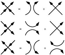
We note that there are indeed three invariant tensors for the case of . The corresponding projectors are . They project respectively on two one dimensional representations, and on a single two dimensional one.
The parameter covers the interval as . Changing is well known to change the exponents of 6 vertex model, and therefore eq. (2.2) for exhibits a critical line, which is in fact in the universality class of the continuous XY () model in the low temperature (Kosterlitz Thouless) phase.
All what was said so far can be easily generalized to the case of spins taking values on a supersphere . The fugacity of loops is now equal to : this combination is the number of bosonic minus the number of fermionic coordinates, and follows from the usual fact that when contracting fermions along a loop, a minus sign is generated 33 3 The generalization of results for models to the case of orthosymplectic groups dates back to the work of Parisi and Sourlas [12]., see sec. 3.3. The loop model formulation therefore provides a convenient graphical representation of the discrete supersphere sigma models for all , in particular where interesting physics is expected to occur. This physics was explored in [11], and the expected results were obtained for . The purpose of this paper is to explore the more challenging case.
Of course, at the naive level of partition functions and without worrying about boundary conditions, it looks as if there is no difference between the spin model and its supersphere cousins provided . The point is that the observables of the models are different or, at the very least, come with different multiplicities. Indeed, consider for instance correlation functions of spin variables. In the case, the spin has only two components , so one cannot build a totally antisymmetric tensor on three indices. This means that the corresponding operator (which has a nice geometrical interpretation to be given in the next paper) will not be present in this case, though it will be in the model when . Note that in general, correlators involving spins within the first bosonic and the first fermionic labels will be the same for any choice of group with and .44 4 Provided, of course, that the boundary conditions imposed on the bosonic and fermionic degrees of freedom are the same in both cases. This is immediately proved by performing a graphical expansion of the correlator: variables outside of the set of the first bosonic and the first fermionic labels are not getting contracted with the spins in the correlators, and cancel against each other in the loop contractions.
A standard trick to extract the full operator content of a model is to study the partition function with different boundary conditions. Consider for instance the spin model on an annulus with some symmetry preserving boundary conditions in the space direction. With what we will call periodic boundary conditions (corresponding to taking the supertrace of the evolution operator) in the time direction, representations of will always be counted with their superdimension, and the partition function will be identical with the one of the case. But if we take antiperiodic boundary conditions, we will get a modified partition function (in the sense of [4]) which is a trace over the Hilbert space instead of a supertrace, counts all observables with the multiplicities (not supermultiplicities), and will turn out to be a very complex object.
A good algebraic understanding of the lattice model will be essential to make further progress, and, since the area is largely unexplored, this will occupy us for most of the rest of this first paper.
3 Transfer matrices and algebra
3.1 Transfer matrices
As discussed briefly in the introduction, the spin model we consider is most easily defined on a square lattice with degrees of freedom (states) on the edges and interactions taking place at vertices. The set of states on every edge is a copy of the base space of the fundamental representation. Interactions at a vertex can be encoded in a local transfer matrix acting on and commuting with the supergroup action. We call an intertwiner and write .
The Boltzmann weights of the model are components of the transfer matrix along a basis of intertwiners. A natural choice of basis are the projectors onto irreducible representations appearing in the decomposition of the tensor product of two fundamental representations. To find them one can apply the same (anti)symmetrization and trace substraction techniques used for reducing tensor representations. If is a mod 2 graded set of basis vectors in with grading , the decomposition of will read
| (3.1) | ||||
Here is the invariant tensor, , and (resp. ) if is fermionic (resp. bosonic). Each of the three terms on the l.h.s. of (3.1) transforms according to an irreps of , or, in other words, belongs to a simple module.
Introduce the identity , the graded permutation operator (also known as braid operator), and the Temperley Lieb operator (proportional to the projector on the trivial representation),
| (3.2) |
In terms of projectors onto irreducible modules, eq. (3.1) may be written in a more elegant way as
Let denote as usual the inversion of space, the inversion of time and the charge conjugation with the matrix . One can check directly from definition (3.2) that is , and invariant, while is and invariant. Moreover, and transform into each other under the rotation of the lattice , while and are related by the crossing symmetry
Take , and as basis of intertwiners in . The local transfer matrix generally depends on three independent weights , and . However, on a homogeneous and isotropic lattice one can normalize and leave only the weight . Finally, the local transfer matrix takes the form
| (3.3) |

On a diagonal lattice with open boundaries represented in fig. 4 choose the time in vertical direction. The notation of sites at a fixed time is such that the left edge and right edge meet at vertex . Let denote a transfer matrix acting nontrivially only at vertex according to eq. (3.3). From the figure it is clear that odd and even times are inequivalent. The transfer matrix , propagating one step forward at equivalent times, may be written as a product of one layer transfer matrices
| (3.4) |
schematically shown in fig. 4.
The simplest way to define a partition function that depends on the whole spectrum of the transfer matrix is by taking the trace of at a certain power . Selecting other boundary conditions with some nontrivial symmetry generally amounts to restricting the whole space of states of the model to a subspace compatible with the symmetry of chosen boundary conditions. What exactly we mean by “symmetry of boundary conditions” will be explained later in sec. 3.3. For the moment let us just say that it is convenient to consider a more general class of boundary conditions, called quasiperiodic, in which is “twisted” by the action of an element of the supergroup. Define the quasiperiodic partition function to be
| (3.5) |
We must take the supertrace in eq. (3.5)
if we want the quasiperiodic partition function to be well defined.
For instance, when we get the usual trace partition function and when
equals to the identity matrix we get the supertrace partition function.
Note that because is a
supermatrix, the tensor product in has to be graded,
that is
After inserting the local transfer matrix from eq. (3.3) in eq. (3.4) and expanding the transfer matrix , the quasiperiodic partition function reads as a sum of weighted products of ’s and ’s. Such linearly independent products must be considered as words of a transfer matrix algebra, while intertwiners and are generators of this algebra. In the next section we identify this algebra as a representation of the Brauer algebra.
3.2 The Brauer algebra
For an abstract introduction to the Brauer algebra see ref. [13, 14] while in the context of centralizer algebra see ref. [15]. We collect in this section some well known facts about the Brauer algebra we shall use in the next sections.
Let and , act nontrivially as and in eq. (3.2) only at the sites of . One can check that for and so defined the following relations hold:
| (3.6) | |||
In the second line of these relations and are supposed to be nonadjacent sites.
Relations (3.6) (is one of the many ways to) define the Brauer algebra (also denoted sometimes by the names of braid-monoid algebra or degenerate Birman-Wenzel-Murakami algebra [16, 17, 18]). Note that this algebra depends on a single, generally complex, parameter , and contains the maybe more familiar Temperley Lieb algebra, generated by ’s alone, and the symmetric group algebra, generated by alone.
For fixed and big enough, the spin models provide highly unfaithful representations of the Brauer algebra . This is because, in , the generators and satisfy additional higher order relations on top of (3.6).55 5 This situation is similar to what happens for models with symmetry in the fundamental representation, and corresponding quotients of the Hecke algebra. For a simple example, consider the spin model on a lattice of width 3. The projector onto the antisymmetric tensor of rank 3 is zero, thus, contains the additional relation . Our spin models in general provide representations of the quotient algebras . The set of relations can be explicitly described for , see [19, 20] and references therein, and we have little to say about the case .
The first step in understanding the spectrum of the transfer matrix brings up the question of irreducible representations, and of their multiplicities in for a particular choice of and . This leads us to discussing some results about the representation theory of the Brauer algebra.

The most natural representation to begin with is the adjoint representation. It admits a diagrammatic representation in terms of graphs on points in which every vertex has degree 1. Usually one orders the points on two horizontal parallel lines as shown in fig. 5. Let denote the vector space spanned on the such diagrams.
The product of two diagrams and is performed by putting on top of and replacing each of the loops in the resulting diagram with . Define diagrammatically the identity and the generators , as represented in fig. 6. One can check that the graphical representation of generators with the multiplication of diagrams satisfy all of the eqs. (3.6). The left action of generators on via the multiplication of diagrams provide the adjoint representation of .

From the graphical representation we see that has a series of invariant subspaces , where is spanned on diagrams with fewer than vertical lines and . The vector space spanned on diagrams with exactly vertical lines may be defined as a module by the coset . The left action of on this modules may be seen as a modified multiplication of diagrams
Under the left action of the algebra the position of horizontal lines in the bottom of a diagram does not change. For a given configuration of the horizontal lines in the top of a diagram and a given pattern of intersections of vertical lines there are possibilities of choosing the configuration of horizontal lines in the bottom of the diagram. This simply means that decomposes into a direct sum of equivalent modules. The coset representative of these equivalent left modules is spanned on graphs on points with every vertex having degree 0 or 1 and a labeling with numbers of free vertices. An example of such a labeled graph is shown in fig. 7. If the labellings are omitted the resulting graph is called a partial diagram.
The labeling of the free points of a labeled graph is a permutation in the symmetric group . The labeled graphs will provide a representation of the Brauer algebra, which is irreducible for generic values of , if we take the labellings in an irreducible representation of . We call such representations generically irreducible. Let be a partition of , which we write as . In a more algebraic language the definition of generically irreducible left modules translates to
| (3.7) |
where is an irreducible module. In view of later numerical analysis we give below a basis in and describe the action of on this basis.

Let denote the labeling of a partial diagram with the permutation , be a set of basis vectors in and be the matrix of the permutation in the representation . A natural basis in is given by all pairs . The action of a diagram on a basis vector is
| (3.8) |
where is the labeling of and is the partial diagram labeled with the identity permutation. The dimensions of is .
In simple words, a generically irreducible module is a span on graphs on points, obtained by choosing points among , pairing all the others (this gives the multiplicity since intersections are allowed), choosing for the unpaired ones a representation of the permutation group and setting to zero the action of any Brauer diagram that reduces the number of unpaired points.
The generically irreducible representations labeled by , appear in the decomposition of the adjoint representation with multiplicity given by their dimension when is semisimple.
Let us conclude with a few words about the reducibility of generically irreducible modules . For integer and a number of strings the Brauer algebra is not semisimple and, as a consequence, certain of the modules become reducible, though they remain indecomposable.66 6 We adopt here the physicist’s habit of calling indecomposable a module which is reducible though not fully reducible. Therefore the set of indecomposables does not contain the irreducibles, unlike in most of the math literature. The irreducible components appearing in such reducible modules are far from being understood (the situation is much worse than in the case of the nonsemisimple Temperley Lieb algebra [21, 22]). Numerical computations based on the diagonalization of the transfer matrix in the diagrammatic representation of restricted to decreases in efficiency very fast with increasing , compared to the ideal case where the transfer matrix is restricted to an irreps of . This is because for big and fixed the number of irreducible components in “goes wild” and there are a lot of “accidental degeneracies” in the spectrum of the transfer matrix restricted to .
However, a significant progress in this direction has been recently made in [23, 24]. Let us note that, as described in [23], the content of (at least some) ’s can be computed by repeated applications of Frobenius reciprocity applied to the short exact sequence of [14] describing the structure of the induced modules .
In the end we recall the basic results for the Temperley Lieb algebra, to allow a quick comparison with Brauer. Temperley Lieb algebra diagrams are a subset of Brauer algebra diagrams subject to the constraint that no intersections between edges are allowed. The dimension of the algebra is given by the Catalan numbers . The main line of reasoning for finding generically irreducible modules follows the same way, except there is no available action of the symmetric group on vertical lines. Therefore, the analogue of the labeled graphs will be the partial diagrams, in which no free points may be trapped inside an edge. The number of such graphs is , where is the number of edges. The generically irreducible modules are parametrized by the number of free points in the graphs.
The presented facts about the Brauer algebra should be enough to understand the loop gas reformulation of spin model, which we give in the next section.
3.3 Loop reformulation of spin models: the algebraic point of view

The emergence of dense intersecting loops becomes transparent if we take the local transfer matrices in the adjoint representation of the Brauer algebra. This simply amounts to replacing in eq. (3.3) the generators , and defined by eq. (3.2) with the diagrams in fig. 6. The adjoint local transfer matrix is represented in fig. 8.
We now define a loop model on a diagonal lattice represented in fig. 4, with reflecting boundaries on the left and right (ie, free boundary conditions in the space direction) and identified boundaries on the top and bottom (quasiperiodic boundary conditions in the time direction.) The states of this model are coverings of the lattice with dense intersecting loops. Dense means that every edge on the lattice necessarily belongs to a loop. Avoiding loop vertices have weight 1 and intersections come with weight . There are two possible ways for a line to close in a loop. The first one comes from the graphical representation of the relation in fig. 9. We call such loops bulk loops. Clearly the fugacity of bulk loops is fixed to by the Brauer algebra. The second possibility is that the ends of the line close in the identified points of the top and bottom boundaries of the lattice. We call such loops cycles. The boundary condition we consider have an annulus geometry and, thus, a cycle can be either contractible or uncontractible. The fugacity of cycles is not fixed by the algebra. In fact, as we explain below, this is exactly the degree of freedom allowing for multiple mappings from the spin models with fixed and the dense intersecting loop model with fugacity for loops.
We start by evaluating the trace of a diagram in the spin representation and then we generalize the result for quasiperiodic boundary conditions given by . We follow the same line of reasoning as in [13].
A cycle in a diagram is the subgraph on the set of points belonging to a loop if we identify its top and bottom vertices. By an abuse of language we call the corresponding loop also cycle. If we put a diagram to the left of a diagram we get a new diagram which we denote . Let be the cycles in . We can separate them by permuting the top and bottom vertices of with the same permutation
Thus the trace of a diagram depends only on the weights of cycles
More than that, the weight of a cycle depends only on how many times it winds the annulus.
Indeed, if a cycle on points has no horizontal lines, then, by applying the same permutation to the top and bottom vertices we can bring it to the cycle . This is because permutations with one cycle are conjugate in .

If a cycle has a horizontal edge between the first and the second vertex in the top then it has the same weight as a certain cycle on four points less then
| (3.9) |
If we compare the on the left with on the right
![[Uncaptioned image]](0801.0430v1/contr.png)
it is clear that, in the end of the iterative application of eq. (3.9), the final cycle can be interpreted as being the initial cycle maximally contracted on the annulus.
In the end, the only weights we need to compute explicitly are that of the cycles and
For boundary conditions twisted by the matrix the generalized weights are computed to be
| (3.10) |
In the fundamental representation, every supermatrix is diagonalizable. The diagonal form of in the fundamental representation is determined by exponentiating elementary weights and introduced in sec. A.1. Thus, restricted to has eigenvalues and restricted to has eigenvalues . The braces in mean that appears for odd only. Eq. (3.10) can now be rewritten
| (3.11) |
For only the eigenvalues in change with respect to the previous case. There are of the form for odd, while for even and . Instead of eq. (3.11) one has now
To summarize the basic results in this section, let be a dense loop covering of the lattice, be the number of intersections, be the number of bulk loops, be the number of contractible loops (cycles) and () be the number of loops winding the annulus an even(odd) number of times.
On the annulus the trace partition function (which would correspond to antiperiodic boundary conditions in the (imaginary) time direction) of the spin model may be reformulated as a dense intersecting loop model in the following way
| (3.12) |
We see that it does depend on separately and not only on .
Meanwhile the supertrace partition function (which would correspond to periodic couplings) reads
where is the total number of “loops” and, since it depends on only, is the same as for the model. One can say that taking the supertrace in the partition function is equivalent to restricting the supersymmetry of the spin model to a, smaller, symmetry.
Denote the spectrum of the transfer matrix of the spin model by . We have the following important inclusion property
| (3.13) |
The only difference between the and quasiperiodic partition functions is the weight of uncontractible cycles. For a matrix with eigenvalues and , except , the weight of uncontractible cycles is, according to eq. (3.11) either or . Notice that these are exactly the weights of uncontractible cycles in the trace partition function for the spin model, which proves eq. (3.13).
We will use the inclusion property (3.13) in the next section to derive some information about the indecomposable representations of appearing in the decomposition of .
4 Decomposition of
4.1 General results
Assume the transfer matrix be a generic element of . The action of on the tensor space was defined in the beginning of sec. 3.2. The complete picture of the reducibility of the transfer matrix can be conveniently encoded in the decomposition of into a direct sum of indecomposable modules
| (4.1) |
where denotes the multiplicity of isomorphic indecomposable modules (it does not depend on ), and the set is defined implicitly by the formula, and will be defined explicitly below. We remind the reader that is not necessarily a semisimple module if , so the modules appearing on the rhs of eq. (4.1) can be reducible.
The question of computing degeneracies of eigenvalues of the spin transfer matrix is easier to treat by looking at the centralizer , which acts on from the left if one consider acting from the right. The dimension of indecomposable modules in the decomposition of as a -module
| (4.2) |
will give the desired degeneracies. This is due to the fact that are dimensions of simple modules appearing as constituents of in eq. (4.1), while are dimensions of simple modules appearing as constituents of in eq. (4.2). Taking the character of both eqs. (4.1,4.2) one can see that the number of irreducible components in is equal to the number of irreducible components in .
Because the action of commutes with we have that . However, when is semisimple it follows from the Wedderburn decomposition theorem that . In the following we suppose that there is still a Schur duality between and the quotient of faithfully represented on . This allows us to give an algorithm to compute the lhs of eqs. (4.1,4.2) for small tensor powers and get some intuition about the general structure of and .
The set of partitions labels irreps, while selects those of them which do realize on the tensor space . Denote by the double sided ideal defined by . The annihilator is diagrammatically described in [20]. Under the homomorphism , the indecomposable modules give rise to induced modules . Clearly, is a tensor representation and can be generated by trace substraction and symmetrization as
| (4.3) |
where , extracts all the traces from the tensor space and acts nontrivially only on as a Young symmetrizer. The double sided ideal is completely characterized by the set of weights . Note that . The surviving indecomposable tensor modules are given by with irreducible components removed. The quotient can be carried out by imposing the vanishing of all words with . It is useful to notice that not all of these conditions are independent and as one can see from eq. (4.3) if .
As discussed in sec. A.1 and A.2, the irreducible components of are indexed (up to an equivalence under the action of the outer automorphism induced by the symmetry of the Dynkin diagram of when even) by the set of hook shape partitions. Representing the supergroup as a semidirect product , the elements of naturally acquire the structure of a couple of the form or if and if , where are the trivial, alternating (superdeterminant) and two dimensional representations of . Thus, every gives rise to two inequivalent irreps with highest weights and the associate if and a single self-associate irreps of highest weight if . For typical , one can realize the irreps on tensors and describe their symmetry by some Young tableaux. As discussed in details in sec. B, the Young tableau corresponding to can be constructed by adding a border strip to the Young tableau of shape corresponding to . Ultimately, this is justified by the fact that eq. (4.5,4.6) gives the right characters for and that they coincide up to . Although atypical representations cannot be realized as tensor representations we represent the associate weight of an atypical weight by a Young tableau such that is a skew partition described in sec. B and sec. C.
The idea is to exploit the fact that the characters of indecomposable modules , given in [13], do not depend on the semisimplicity of . This and some properties of generalized Schur functions, which are summarized in [15], can be used to prove that
| (4.4) |
is true even for all . Here is the character of in the representation provided by . The functions are polynomials in the eigenvalues of , which where introduced for the first time by Bars in [25] in an early attempt to describe the supercharacters of . They can be defined recursively as
| (4.5) |
and
| (4.6) |
For the Brauer algebra is semisimple and . Consequently, are irreducible and . Because of the commuting actions of and one can naturally consider as a --bimodule, with acting from the left and from the right. Then, eq. (4.4) can be understood as a consequence of the decomposition
| (4.7) |
with being actual characters of tensor irreducible modules as shown in [15].
For such that , the polynomials cannot generally be interpreted as the character of some representation. As we have seen in sec. 3.3, can be brought to the form and eq. (4.4) is not more then a simple equality between two polynomials in eigenvalues of . Moreover, the two eqs. (4.2,4.4) are still compatible, even if there are much more elements in then in . This is possible because are not functionally independent when . Then, for the polynomials can be written in terms of functionally independent with by means of modification rules for characters
| (4.8) |
The fundamental eq. (4.4) is useful for small widths , when it is possible to compute the number of irreducible components in either by repeated applications Frobenius reciprocity, as explained in [23], or by numerically diagonalizing the transfer matrix of sec. (3.1) in the adjoint representation of and detecting the “accidental degeneracies” in its spectrum. Indeed, from the explicit definition (3.7) it is clear how to restrict the adjoint transfer matrix to indecomposable modules . After we described in details the action of generators on the basis of in sec. 3.2, the algorithm of a numerical diagonalization is straightforward.
The information about the structure of and the modification rules in eq. (4.8) can now be used to bring eq. (4.4) to the form
| (4.9) |
We see that iff 77 7 Although , are not irreducible characters, one can still use them as a basis for representing the character of any representation. there is at least one such that . To determine one has to decompose the factor of in eq. (4.9) as a sum of irreducible characters, which are explicitly known, as far as we know, only for and . Given the huge order of the set of weights , it may seem that calculations according to eq. (4.9) are extremely cumbersome already for small . The simplifying point is that (or ) is non zero only if both weights are in the same equivalence class of (or ). The splitting of (or ) into equivalence classes, called blocks and described in details in sec. B, is with respect to an equivalence relation between irreducible components of indecomposable (or ) modules.
An important consequence of the fact that supertrace partition functions depends only on the part of the spectrum is the vanishing of the superdimension for all indecomposable modules with . A more restrictive criterion for supercharacters deriving from the full inclusion sequence in eq. (3.13) can be derived by taking a matrix with eigenvalues and for , . Then, it can be seen from eqs. (3.11,3.12) or eqs. (4.5,4.6,4.4) that any quasiperiodic partition function will also be an quasiperiodic partition function. As a consequence and the supercharacters of vanish when and can be embedded in .
For the modules is semisimple. Therefore . On the other hand, if is big enough . It could be interesting to understand the relation between the sequence and the cohomology of the radical .
Observe that a filtration similar to that of is available on by the degree of atypicality of its elements. In fact, we explain in sec. B of the appendix how the weights in a block of or can be organized by the number of removable balanced continuous border strips in the corresponding Young tableau. This number can be interpreted as the degree of atypicality when the corresponding partition represents an weight.
4.2 spin model
Let be a two dimensional vector space endowed with an action of . The action of on the tensor space is
acts according to the following definition of generators
where have the following representation on
| (4.10) |
(note that differs in some essential way from the projection operator onto the singlet representation in the usual basis). The decomposition of as a --bimodule is simply
| (4.11) |
Here
The tensor representations are irreducible with dimensions and . The representation is the trivial one and is the associate one dimensional representation. At the restriction to the representations and become equivalent, while splits into two nonequivalent one dimensional representations where is the angle. The representations are irreducible as well and are constructed by acting with on the tensor module in eq. (4.3). The dimensions of simple modules are easily computed by looking at the first row of , where is the fusion matrix
| (4.12) |
described by a type Dynkin diagram with labeling of the nodes shown in fig. 10. It is not hard to solve the recurrence relations satisfied by
and get that except the case when is even and for which . These are, as expected, the number of eigenvalues of the transfer matrix for the 6 vertex model in the sector of spin .

We are interested in giving an algebraic description of the 6 vertex model transfer matrix algebra. In other words we want to identify the Brauer algebra annihilator of and carry out the quotient .
All the weights such that satisfy either or . Thus, it is enough to consider and impose the vanishing of the double sided ideal of the word projecting onto . As explained in the beginning of the previous section , where extracts all the traces from and are the Young symmetrizers corresponding to .
The projector can be found by looking at the form of an arbitrary tensor after extracting all of its traces
which gives
and clearly .
The Young symmetrizer is
and , where
are the projectors onto the standard Young tableau and . The two orthogonal projectors and are independent only if we restrict to the right action. In fact, the left ideal of the word is the same as the double sided ideal of the word .
The condition gives the following restriction
| (4.13) |
on generators . Putting one can see that eq. (4.13) implies that are Temperley Lieb operators with . There are no more restrictions that can be drawn from the conditions , because is a one dimensional projector.
Before exploring the next vanishing condition let us revise the the defining relations of given in eq. (3.6)
| (4.14) | ||||
| (4.15) | ||||
| (4.16) |
which imply
| (4.17) | ||||
| (4.18) |
Observe that although the algebra has now two Temperley Lieb operators their role is not symmetric yet at this stage.
Next, the condition implies
which after inserting with the help of eqs. (4.15,4.18) becomes
| (4.19) |
Multiplying eq. (4.19) by on the right we get:
| (4.20) |
which can be used to rewrite eq. (4.19) as
| (4.21) |
Multiplying by on the left and on the right of eq. (4.21) and using only the relations between , the relations between and eq. (4.14) one can get all the eqs. (4.15–4.20) and also
which establish a complete symmetry between and .
The double sided ideal of is composed of four linearly independent words — two generated by the left action and other two generated by the right action of . It is useful to note that after taking the quotient of we are left with 10 independent words instead of 15, which is exactly what we need for the 6 vertex local transfer matrix.
We give the following abstract definition to the 6 vertex model transfer matrix algebra in term of generators
| (4.22) | ||||
| (4.23) | ||||
| (4.24) | ||||
The defining relations are symmetric under the transposition , which changes the multiplication order, under the reflection and under the involution . Thus, if then , and is also true for any word .
Introducing the operators , with the property , one can rewrite eq. (4.20) as
Thus, one can eliminate all of the generators and leave only subject to satisfy
| (4.25) | ||||
Denote by the extension of the ordinary Temperley Lieb algebra, generated by , with the additional generator satisfying eqs. (4.25). We see that and are isomorphic algebras. The graphical interpretation for the reduced words (products of generators of minimum length) of and its relation to the blob algebra and the Temperley Lieb algebra of type is discussed [27]. The generators are diagrammatically represented as usual, whereas is represented as with each of its horizontal edges marked by an involutive blob as shown in fig. 11.

An unblobbed loop is identified with 2, while a blobbed loop with 0. Thus, we see that is a subalgebra of the blob algebra composed of all planar diagrams on points with an even number of blobbed edges. The dimension of is, as explained in [27], half the dimension of the blob algebra, that is .
There are several important consequences arising from the isomorphism between and from the point of view of integrability. First of all, we check that indeed the solution to the Yang-Baxter equation
| (4.26) |
provided by the algebra coincides with the well known XXZ spin chain -matrix.
For that, consider the ansatz and plug it in eq. (4.26). Choosing as basis set in the 10 words we get two independent functional equations
| (4.27) | ||||
| (4.28) |
where . The primed functions are evaluated in , the unprimed in and the double primed in . All other words provide the same third equation, which is a consequence of eqs. (4.27,4.28). The solution to the system of eqs. (4.27,4.28) is
| (4.29) | ||||
| (4.30) |
with an arbitrary constant . Taking and in the representation provided by the eq. (4.10) we find the famous XXZ spin chain -matrix
| (4.31) |
as expected.
Clearly, an integrable system in has to be related to an integrable system in because of the isomorphism of these two algebras. However, the ansatz plugged into the eq. (4.26) gives only the isotropic point () solution . The only possibility to give a richer content to the integrability in is by introducing nontrivial boundary conditions. This means that the anisotropy of the XXZ spin chain can be generated by introducing nontrivial boundary conditions at the isotropic points, an observation made earlier from a slightly different perspective in [28].
4.3 spin model
The representation theory of the superalgebra is summarized in [29]. As we have already mentioned, all of irreducible characters have been computed and indecomposable representations classified. We give a brief reminder of these results in sec.A.3 and make some remarks, based on the general discussion in sec. A.2, on the difference between the representation theory of the supergroup and its Lie superalgebra.
The tensor space , seen as a module, can be represented as a direct sum of a part “lifted” from
| (4.32) |
and a projective part
| (4.33) |
where is the projective cover of . This decomposition can be proved by induction on using two facts:
- •
The tensor product between atypical irreducible representations with highest weights labeled by one row partitions (see bellow) and decomposes to 88 8 Modulo irreps labeled by , this decomposition provides the same fusion matrix as eq. 4.12. Thus, multiplicities in are the same as those in . Rather then a coincidence, this is a direct manifestation of the algebra inclusion at the level of dimensions of irreps.
This is proved by counting the dimensions on the right/left hand sides and, then, observing that is typical and , being in different blocks, cannot give rise to indecomposables.
- •
The tensor product of a projective module with any other module is projective, thus, decomposing to a direct sum of projectives.
In the following we use the fundamental eqs. (4.4,4.9) to decompose as a module and verify the assumption that by comparing the result to eqs. (4.32,4.33).
The conditions of atypicality for a weight are given in sec. A.3. In the partition notation we adopt, these are equivalent to
Typical weights satisfy none of atypicality conditions listed above. Note that typical representations are irreducible, have vanishing superdimension, and are simultaneously projective and injective. This means they cannot be a constituents of any other representations without being a direct summand. One can say they are “their own blocks”.
The supercharacters of associate irreps satisfy . For typical weights, the polynomials give the right irreducible character. Because of the modification rules, see sec. C, it is possible to define a partition such that . Therefore, it is convenient to identify the associate weight with the partition . The Young tableau of can be constructed by replacing the orthogonal part of the Young tableau of by its associate, that is by putting and leaving all other columns unchanged. For instance . Exceptions are the typical weights such that . The only such weights are or and we put and .
The atypical weights can be labeled by two integers and , where denotes the isomorphism class, also called block.
In the partition notation, the block is composed of weights and . The associate block is composed of weights and .
The self associate blocks are composed of weights ( for and for ), for and for .
With the given notation for associate weights one can check with the help of [29] the following decomposition of polynomials as a sum of supercharacters
| (4.34) | ||||
This is done in two steps. First one show that eqs. (4.34) hold for a supermatrix with .99 9 To compare with [29] one has to take the eigenvalues of of the form At this step is yet impossible to distinguish between associate representations. In order to do so, one has to explicitly construct the elements of the enveloping Lie superalgebra connecting the maximal vectors of irreducible components of indecomposable highest weight modules and, then, look at their symmetry under the outer automorphism . See sec. A.3 for details.
We have just listed all the elements of . Eq. (4.34) is a bijection between and . As a consequence, and weights can be labeled by the same set in the partition notation we have adopted. This is supporting the assumption that there is some sort of exact equivalence between the category of and modules on . Bellow all the weights are partitions and, to avoid confusion, we write if is considered as a weight and if it is considered as a weight.
Let us show that the terms in eq. (4.4) with do not actually contribute to . First note that if cancels out from eq. (4.4) then certainly in eq. (4.3) is a trivial module. Therefore any module will also be trivial if . Second, if does not contribute to eq. (4.4) when then it does not contribute to it for any . Thus, it is enough to prove for every that the weights just greater (by inclusion) then do not contribute to eq. (4.4) when the are allowed for the first time to appear.
Let be a typical (associate) weight. Then, as we show in sec. B, is a minimal partition (with respect to the inclusion in its block). There will be a unique weight just greater then and, a priori, can modify to . It is proved by induction in sec. C that a positive sign would imply atypicality conditions on and, thus, . Moreover, from [23] we know that has one composition factor . Taking , we see that the contribution to eq. (4.4) of from cancels out with the one from .
Before proceeding to nontrivial blocks we need to know the number of irreducible components in . According to [23], the graph representing the partial ordering (by inclusion) of weights in a block determines the required information about the content of modules . The ordering graph is represented in fig. 12.
Now, let be an atypical (associate) weight. Then, any weight such that satisfies , with represented by a white dot in fig. 12.

The explicit form of is and . Next, one can check with the help of modification rules that
| (4.35) |
vanishes identically. Further, from fig. 12 each of the modules has a single irreducible component . Finally, taking one can see from eq. (4.35) that the contribution of to eq. (4.4) cancels out.
Let us introduce the compact notations and . Then, putting together eq. (4.34) and fig. 12 we get from eq. (4.4) the following content of indecomposable modules appearing in eq. (4.2)
| (4.36) | ||||||||||||
where and . The indecomposable modules are represented below and it should be understood that they get “paired up” in the decomposition of as a bimodule.1010 10 In pedantic terms, the pairing can be represented by the functor sending left modules to left modules. Alternative, maybe more intuitive physically, representations of the blocks will be given in the next paper.
The structure of modules is in perfect agreement with eq. (4.32,4.33). We recognize in the first term of eq. (4.36) the contribution to , while the rest of the terms are exactly the projective modules appearing in , that is and .
For typical , the modules are irreducible and get paired up with in the decomposition of as a --bimodule.
Observe that, as expected, only the modules (which coincide with in eq. (4.11)) contribute to the supertrace . Indeed, typical modules modules have superdimension 0. The same is true for projective modules. One can explicitly check from eq. (4.36) that if we take into account that only fermionic generators connect irreducible components of indecomposable modules. For instance, .
As we have explained at the beginning of sec. 4.1, the degeneracies of the eigenvalues of the spin transfer matrix are given by . We compute them in app. A.3.
Thus, in conclusion we see that and, because is by definition a faithful module we also have . In other words, the two algebras and are the full centralizers of each other on .
This results allows us to relate the decomposition of as a left module to the decomposition of as a right module.
Collecting in a single indecomposable module all factors in eq. (4.36) which correspond to (happen to be above) an irreducible component we get 1111 11 Again this “collecting” can be represented by the functor sending left modules to left modules.
| (4.37) | ||||||||||||||
where and the content of is represented below .
5 The hamiltonian limit
It will turn out in our forthcoming analysis of conformal properties to be easier to study numerically the hamiltonian
The expectation — which we will confirm in great details — is that this hamiltonian will be in the same universality class as the spin model we had started with.
The hamiltonian is obviously local and has only nearest neighbour interactions if the ’s and ’s are taken in the spin representation provided by eq. (3.2). However, this is no longer true if we think of as an element of the adjoint representation of .
The lowest eigenvalue of belongs to the irreducible representation labeled by .
For generic it is nondegenerate if is even and has degeneracy if is odd. On the other hand, the highest eigenvalue belongs to the completely antisymmetric representation labeled by . In this representation the ’s act as -1 and the ’s as 0.
The hamiltonian is determined up to an arbitrary additive constant and multiplicative factor. For numerical diagonalization it is convenient to fix the additive constant such that the maximal eigenvalue of be zero. The multiplicative factor is fixed by requiring
with as in eq. (3.2), as in app. A.1 and being the XXZ spin chain hamiltonian in its usual form
The fact that the eigenvalues of the 6 vertex model appear as a subset of the eigenvalues of the transfer matrix for the model and carries over to a similar result for the hamiltonians. The velocity of sound for the massless excitations can thus be derived from its value for the XXZ subset, which is well known from [30] to be
| (5.1) |
The hamiltonian is diagonalized numerically in the adjoint representation of the Brauer algebra by studying its action on the diagrams just like for the transfer matrices. Next, once the structure of indecomposable modules is known, eq. (4.4) can be used as explained in sec. 4.1 to select the part of the spectrum which does indeed appear for a fixed spin model.
However, in the two special cases the hamiltonian greatly simplifies. In the following two subsections we discuss the behaviour of the spectrum of in the two limits .
5.1 The limit
When the Temperley Lieb operators do not contribute to and, thus, the hamiltonian is no longer a generic element of the Brauer algebra , but belongs instead to the subalgebra . This will translate to additional degeneracies in the spectrum of at the point compared to other points in the range .
Hamiltonians of type , with ’s in the representation provided by eq. (3.2), are integrable and have been studied in [31] and [32]. Although the continuum limit of such spin chains is a gapless field theory, it fails to be conformal, because excitations have a scaling law in the thermodynamic limit. This can readily be seen from the vanishing of the sound velocity in eq. (5.1). We will not enter into the details here, but just mention that the different systems of Bethe ansatz equations are indexed by -hook shape partitions . This is exactly the label of irreducible representations of the group algebra realizing in the centralizer of the spin chain , with being the fundamental representation of . We see that the symmetry of our spin model jumps to at the point .
The additional degeneracies in the spectrum of the spin model at the point can be understood by looking at the decomposition of modules , into a direct sum of irreducible modules . Let and , then it was shown in [33] that the multiplicity of in the decomposition of is
| (5.2) |
where are Littlewood-Richardson coefficients. Alternatively, is the number of tensors of rank , with index symmetry of some fixed standard Young supertableau of shape , that can be obtained from a tensor of rank , with index symmetry of some standard Young supertableau of shape , by contracting indices in all the possible ways.
One can apply eq. (5.2) to understand the degeneracy of the lowest level of at . First, observe that is minimized in the sector (where ’s acts as 1). The only such that are one row partitions. Thus, the lowest eigenvalues of restricted to for become all degenerate at .
Arguments of this kind can be used to derive information about the critical exponents of the spin model in the limit
5.2 The limit
The same reasoning can be applied to the point . At this point, the hamiltonian belongs to the Temperley Lieb subalgebra and the model can be considered as a spin chain where are the fundamental representation of and its conjugate. Additional degeneracies can be understood by looking at the decomposition of modules as a direct sum of standard irreducible modules .
Let us compute the multiplicity of irreducible modules in the decomposition of with .
As explained in sec. 3.2, has a natural basis composed of all possible pairings of partial diagrams with free points and basis vectors of . We say that a horizontal line of a partial diagram is intersected either if it intersects another horizontal line or if there is a free point in between the two ends of the horizontal line. Let us associate to each partial diagram the number of intersected horizontal lines in . It is not hard to see that the span on the basis vectors , with ’s having at most horizontal intersected lines, is a submodule in . If we denote this submodule by there is an obvious filtration of .
Consider the natural action of on the quotient modules . Observe that the action of changes the labeling of free points in a labeled graph if and only if it also reduces the number of horizontal intersected lines. Therefore, is isomorphic to a direct sum of modules . Obviously and, therefore, we get for , for and finally .
Thus, our problem effectively reduces to understanding the action of on the module , which is composed of partial diagrams on points with unlabeled free points.
At a closer look, one can see that the action of on partial diagrams keeps the reciprocal configuration of intersected lines and free points intact. In other words, if is a map that eliminates all the nonintersected horizontal lines from a partial diagram and acts as identity otherwise, then defines an invariant of , that is
To understand the meaning of this invariant let us define a local map between partial diagrams which sends intersected horizontal lines to free points as depicted in fig. 13 and acts as identity otherwise. The local map is applied repeatedly until there are no more horizontal intersected lines left.

It is not hard to see that extends to a homomorphism of modules
In fact, the role of the map is to show that is composed of a direct sum of isomorphic modules, while that of the map is to distinguish between these modules. The set of partial diagrams in splits into subsets of constant and each of these subsets is isomorphic to as a module.
According to what was said before, we get that equals to the number of graphs on vertices and intersected edges. It follows that does not actually depend on and we drop the index in the following. This fact allows, in principle, for an iterative computation of by simply computing the dimensions of the left and right hand sides of the decomposition formula
that is
| (5.3) |
successively for or . One can give an explicit expression for with a little more combinatorial work.
We call a horizontal line an empty cup if its ends are adjacent and simply a cup if there are separated by free points. Observe that all the lines in a partial diagram are intersected if and only if there is at least one free point in each cup. Thus, if the partial diagram has cups with only one free point inside and a total of edges then the remaining free points can be added to the diagram in different ways in such a way that the resulting diagram has only intersected edges. Moreover, the number of diagrams on points with empty cups and a total of edges is again . This is because the condition of no cups in the connection of the remaining edges is similar to the condition of composing a graph with free points and intersected edges. Putting everything together we get a new recurrence formula
| (5.4) |
reducing the problem to the computation of .
Next, we want to find a recurrence relation for by looking at the connectivity of the first point in the partial diagrams on points with intersected edges. The leftmost vertex in the partial diagram has to be connected to some other vertex at position . The connectivity of the points to the left of the point at position 1 is equivalent to that in a partial diagram with intersected edges and a free point except for the case where . Therefore we have that
| (5.5) |
Now, eq. (5.4) yields . Using again eq. (5.5) for we finally get that
| (5.6) |
The solution of the recurrence eq. (5.6) with the initial conditions and is
and coincides with the absolute value of Bessel polynomials
evaluated at .
6 Conclusion
Besides the careful definition of the spin model and its sectors, the main point of this first paper is the algebraic set up necessary to analyze its symmetries. This is a non trivial task since we are dealing with non semi-simple algebras, and that the action of and are meshed through a complex structure of indecomposable representations. The main results are the decomposition formulas (4.36,4.37) for viewed as a and a module. The decomposition in eq. (4.36) has been computed in two essentially different ways: first, by decomposing tensor products between representations and without knowing anything about the Brauer algebra and, second, starting from eq. (4.4) with the assumption that the representations of and on generate the full centralizers of each other (Schur duality). The fact that we arrive at the same result using both methods highly suggests that our assumption about the Schur duality between and on is correct.
When the question of decomposing is addressed in sec. 4.3, the notion of block appears to be a particularly useful concept for organizing indecomposable representations.1212 12 Let us note that the blocks appear already in the representation theory of simple Lie algebras if infinite dimensional representations are allowed. They are precisely the orbits of the shifted action of the Weyl group on the weight lattice. These results will be applied to educated conjectures about the conformal field theory in the next paper.
Although there are many things left unclear about the representation theory of , it is very tempting to speculate the form of the decomposition of . Before making the guess, observe that as a module , where is a direct sum of projectives organized in blocks, while is a direct sum of simples indexed by the same Young tableau (in the partition notation for dominant weights) as the irreps of . More than that, they appear with the same multiplicities as their partners in .1313 13 In is not hard to prove employing the methods we used in this paper and the results of [29] for that the same phenomenon occurs for . In this case is the trivial representation. Therefore, and are similar in all but the internal structure of their simple summands. The similarity between the two modules has to be understood in terms of their centralizers, because these are precisely the objects that do not ‘‘see’’ the internal structure of simples.1414 14 By a corollary of the Schur lemma, if is a simple module for the algebra then . In conclusion, one should have , which is quite natural once there is a Schur duality between and on . It is tantalizing to speculate that as a module , with projective and . Thus, the problem of the decomposition of as a module is reduced to understanding the projective representations of the supergroup, i.e. to finding the quiver diagram for each block. It has been suggested in [34] that the quiver diagram of blocks does not depend on provided the degree of atypicality and the action of the outer automorphism are fixed.1515 15 can act in two ways: either leave invariant all the weights in the block or pairwise transform some of them. The discussion of sec. A.3 suggests that the two types of quivers for a block of and a fixed will give rise to the same quiver for the induced blocks in .
We also succeeded in computing the multiplicity of Temperley Lieb representations in a standard -module . Finally, we gave a combinatorial description of blocks as the set of minimal partitions dressed by balanced removable border strips and have shown that there is a similar description for blocks.
Acknowledgments: This work was supported by the Agence National Pour la Recherche under a Programme Blanc 2006 INT-AdS/CFT. We would like to thank J. Germoni for fruitful correspondence, and J. Jacobsen and P. Martin for useful discussions.
References
- [1] I. Bena, J. Polchinski and R. Roiban, Phys. Rev. D 69 (2004) 046002, hep-th/0305116.
- [2] F. Wegner, Nucl. Phys. B316 (1989) 663.
- [3] M. Zirnbauer,“Conformal field theory of the integer quantum Hall plateau transition”, hep-th/9905054.
- [4] N. Read and H. Saleur, Nucl. Phys. B613 (2001) 409.
- [5] N. Mann and J. Polchinski, Phys. Rev. D72 (2005) 086002 and N. Mann and J. Polchinski; hep-th/0508232.
- [6] N. Read and H. Saleur, Nucl. Phys. B 777, 263 (2007).
- [7] N. Read and H. Saleur, Nucl. Phys. B 777, 316 (2007).
- [8] B. Nienhuis, E. K. Riedel and M. Schick, Phys. Rev. B27, 5625.
- [9] E. Domany, D. Mukamel, B. Nienhuis and A. Schwimmer, Nucl. Phys. B190 (1981) 279.
- [10] B. Nienhuis, J. Stat. Phys. 34 (1984) 731.
- [11] J. L. Jacobsen, N. Read and H. Saleur, Phys. Rev. Lett. 90 (2003) 090601; cond-mat/0205033.
- [12] G. Parisi and N. Sourlas, J. Physique Lett. (Paris) 41 (1980) L403.
- [13] A. Ram, Pac. J. Math. 169 (1995) 173.
- [14] W. F. Doran, D. B. Wales and P. J. Hanlon, J. Algebra 211 (1999) 647.
- [15] G. Benkart, C. L. Shader and A. Ram, J. Pure Appl. Algebra 130 (1998) 1.
- [16] J. Birman and H. Wenzl, Trans. Am. Math. Soc. 313 (1989) 249.
- [17] J. Murakami, Osaka J. Math. 24 (1987) 745.
- [18] M. Wadati, T. Deguchi and Y. Akutsu, Phys. Rep. 180 (1989) 249.
- [19] H. Weyl, “The classical groups”, Princeton University Press (1946).
- [20] F. Gavarini, “On the radical of Brauer algebras”, math.RT/0606501 (2006).
- [21] F. Goodman, P. de la Harpe and V. Jones, “Coxeter graphs and towers of algebras”, MSRI Publications 14, Springer, Berlin 1989.
- [22] P.P. Martin, “Potts models and related problems in Statistical Mechanics”, World Scientific, Singapore (1991).
- [23] A. Cox, M. De Visscher and P. Martin, “The blocks of the Brauer algebra in characteristic zero”, math.RT/0601387.
- [24] A. Cox, M. De Visscher and P. Martin, “A geometric characterization of the blocks of the Brauer algebra”, math.RT/0612584.
- [25] A. Balantekin and I. Bars, J. Math. Phys. 22 (1981) 1149.
- [26] C. J. Cummins and R. C. King, J. Phys. A 20 (1987) 3103.
- [27] R. Green, JKTR 7 (1998) 155.
- [28] D. Levy, Int. J. Mod. Phys. A6 (1991) 5127.
- [29] J. Germoni, Boletin de la Academia Nacional de Ciencias 65 (2000) 147 http://hal.archives-ouvertes.fr/hal-00002750/fr/.
- [30] C. Hamer, J. Phys. A 19 (1986) 3335.
- [31] B. Sutherland, Phys. Rev. B 12 (1975) 3795.
- [32] H. Saleur, Nucl.Phys. B578 (2000) 552.
- [33] P. Hanlon and D. Wales, Math. Comp. 54 (1990) 771.
- [34] V. Serganova Proceedings of the International Congress of Mathematicians, 1998.
- [35] V. Kac, Adv. Math. 26 (1977) 8.
- [36] B. Morel, A. Sciarrino, P. Sorba, J. Phys. A: Math. Gen. 18 (1985) 1597.
- [37] J. P. Hurni, J. Phys. A 20 (1987) 5755.
- [38] R. Farmer, P. Jarvis, J. Phys. A: Math. Gen. 17 (1984) 2365.
- [39] V. Kac, Lecture Notes in Math. 676 (1978) 597.
- [40] V. Kac, Commun. Algebra 5 (1977) 889.
- [41] J. Van der Jeugt, J. Math. Phys. 26 (1985) 913.
- [42] I. MacDonald, “Symmetric functions and Hall polynomials”, Clarendon Press, Oxford (1979), 10
Appendix A Appendix
A.1 Lie superalgebra

In this section we recall standard facts about the Lie superalgebra mainly following the pioneering work of Kac [35]. For more details on Young supertableaux see [36, 37, 38].
Let be a vector space with an additive grading , that is and . Let , and . Choose in a basis with and . We take the vector in brackets because it appears for odd only.
The grading of induces a grading on , that is preserves the degree of and changes it. Define the supertranspose of a matrix by
| (A.1) |
Let denote the matrix with the only nonzero components
| (A.2) |
The Lie superalgebra is realized as a subset of with elements satisfying
| (A.3) |
In terms of elementary matrices the generators of read
| (A.4) | ||||
| (A.5) | ||||
| (A.6) |
The generators span the Cartan subalgebra . Denote by the basis in dual to . It can be easily checked that generators in eq. (A.4) correspond to roots of the type , generators in eq. (A.5) correspond to roots of the type and generators in eq. (A.6) correspond to roots of the type . The bilinear invariant form induces a scalar product on .
The standard basis is recovered by putting for and for . Elementary weights are orthogonal in and . The first simple roots are chosen to be , , for and . The last simple root is for odd and . The roots are called odd and the rest — even.
The component of a weight along the hidden simple root is
| (A.7) | ||||
| (A.8) |
According to [35], an highest weight is dominant iff it has integer Dinkyn labels and integer satisfying the following consistency conditions
| (A.9) | ||||
All irreducible finite dimensional representations are indexed by dominant weights . Given a dominant weight in the standard basis, the first Dynkin labels are for , for . The last Dynkin label is for odd and for even. From eq. (A.7) we also get .
The set of numbers define a partition, shown in fig. 15, provided that consistency conditions (A.9) plus some additional constraints depending on are satisfied. These additional constraints require and to be even if is even, and to be to be even if is odd.

The last two conditions define tensorial weights.
Partitions such that are called hook shape. Let denote the outer automorphism induced by the symmetry of the Dynkin diagram under the exchange of the last two roots in fig. 14. This automorphism is extremely important in understanding the difference between the representation theory of the supergroup and its Lie superalgebra. Note that can be explicitly realized through the discrete transformation exchanging the last two basis vectors in . Indeed, for and because are the duals of . Therefore .
In the case of odd, there is a bijective correspondence between hook shape partitions and dominant weights . The same holds for even, except for with when represents both and .
If there is a pair such that at least one of the conditions below are satisfied
| (A.10) | ||||
| (A.11) |
the weight is called atypical.1616 16 For the highest weight is always atypical. See [39] for the origin of these conditions and note ref. [38], where these have been presented in the form (A.10,A.11). If none of these conditions is satisfied, the weight is called typical and, according to [39], the associated Kac module (which is a finite dimensional quotient of the corresponding highest weight module) is irreducible, its (super)character is given by the Weyl-Kac formula [40] and, in particular, its superdimension is zero.
A.2 supergroup
Let be a Grassman algebra. The supergroup may be realized as a subset of even supermatrices
with entries in and belonging to , and entries in and belonging to , which satisfies
| (A.12) |
Equivalently, can be seen as the set of linear transformations leaving invariant the graded symmetric form
| (A.13) |
where are arbitrary points in a superspace parametrized by coordinates and and .
Representing with infinitesimal and expanding eq. (A.12) one gets the definition (A.3) of the superalgebra . Thus, the subgroup of connected to identity is an exponential of . The representation theory of both is the same as long as we restrict to tensor representations which are the only ones appearing in the tensor space .
From the definition (A.12) any matrix has superdeterminant . The supergroup has two disconnected parts , which correspond to the value of the superdeterminant of its elements, that is .
To see this, one can repeat the same reasoning typical of groups. Elementary transformations susceptible to change the sign of the superdeterminant belong to the discrete symmetry group of the invariant form (A.13). The generators of are read out from eq. (A.13) to be “reflections” and , and permutations and . For odd there is also the reflection . The subgroup is in fact the Weyl group of the root system of . Denote by the set of elements of embedded in . It is easy to see that all elements of are conjugate in to a single reflection , which one can take if is even and if is odd. Therefore, we see that indeed .
Let be a vector of weight . Then, as seen in sec. A.1, there is an action of on provided by . In the case of the outer automorphism exchanges with . The representations induced from to are of the form
| (A.14) |
There are two possible cases now: i) either and then obviously with and or ii) and the induced module in eq. (A.14) is irreducible.
Two representations of are called associate. The modules and are also called associate. In contrast, is isomorphic to its associate because there is an equivalence transformation between and through the change of sing of basis vectors in the subspace . Therefore is called selfassociate.
A direct implication following from the definitions of (self) associate modules is , where are (self)associate weights of . For a selfassociate weight this equality implies if .
Note that the centralizer of on is the direct product algebra rather then . This algebra has the same tensor irreducible representations as the supergroup .
A.3 Lie superalgebra and supergroup
This is a compact resumé of the results presented in [29] plus some additional remarks on the representation theory of .
The superalgebra has minor differences with respect to the general context of superalgebras, because of the isomorphism . The even part of the superalgebra is . The odd part is a representation of the even part of dimension .
The standard basis vectors of are normalized as . The even and the odd positive root systems are and . The simple roots are traditionally chosen as , , . The hidden root will then be .
Consistency conditions (A.9) for a dominant weight , require and . We associate to a hook shape partition with symplectic part and orthogonal part . To make the correspondence bijective we mark the partition by when .1717 17 Any irreps can be written as a couple of irreps. The sign attached to distinguishes between and when .
Atypicality conditions (A.10,A.11) take the form
The solutions can be parametrized by two integers and . For these are , while for , and .

Denote by the simple modules. For typical and can be computed by decomposing into (at most 16) representations of
The dimensions of can be computed with the help of character formulas given in [29].
For we get , and , where .
For we get and , and .
The set of weights with fixed belong to the same block of . To (at least partially) see this one has to check that the second order Casimir invariant takes the same value on the whole block .1818 18 The second order Casimir is a central element of the enveloping superalgebra. The eigenvalues of central elements on define the central character of . If two weights are in the same block then have the same central characters. This is a consequence of the extension of the Schur lemma (in the form known to physicists) to indecomposable representations. The actual construction of the set of indecomposable modules providing the equivalence relation of sec. B between the weights of a block is done in [29].
The quiver diagram representing the structure of projective modules in a block is represented in fig. 16. The projective covers of the modules in the block have the submodule structure
| (A.15) | ||||||||||||
while in the block their submodule structure is
| (A.16) | |||||||||
The dimensions of projective modules in the block are , while in the block there are . The superdimension of projective (including typical) modules vanishes.
Let us apply the general discussion of sec. A.2 to the supergroup . The outer automorphism acts on by exchanging with . Consequently, for or and otherwise.
We claim that the quiver diagram of type for the block of will give rise to two quiver diagrams of type , as shown in fig. 17, and, consequently, to two associate blocks for the algebra , which we call . As we shall see bellow, the weights in the block are , while the weights in the block are .
We also claim that the quiver diagram of type for the block of will give rise to a single quiver diagram of type , as shown in fig. 17, and a selfassociate block for the algebra , which we label also by . As we shall sea bellow, the weights in the block are .

Our claim follows from the analysis of shift operators introduced in [41]. These operators are very practical for decomposing Kac modules into irreps.1919 19 The fact choose Kac modules in order to understand the transformation properties under of arrows in the quiver diagram of a block is irrelevant for the following. One can take instead of the standard modules as well, which are defined by cohomological induction in [29]. To be more specific, let be a vector of weight maximal for the algebra . Then, is again a maximal vector of weight for . To identify irreducible components in one has to search for maximal vectors with dominant weights in the same block as .
Consider first the block of . Then has a maximal vector and one can check that all positive odd generators annihilate it. Therefore is a maximal vector for and contains at least and . In fact, these are the only two irreducible factors of because, using the Weyl-Kac formula for characters and the results of sec. A.3, one can check that . In the case one has that and, therefore, contains also the trivial representation.
In order to see how the four weights split into two different blocks of one has to check out how transforms under the action of . From the explicit expression of shift operators in [41] it follows that and, consequently, are in the same block and are in an other same block of .
The module has a maximal vector , of weight zero, corresponding to the trivial representation . With the help of relations in appendix [41] for the shift operator products of type , one can show that and, therefore, belongs to the block of as claimed.
Consider now the block of . Then will have a single maximal vector (besides ) corresponding to the irrep given by if , if and if . The induced module will be the sum of glued together by the action of . Finally, the induced module has two irreducible components and with maximal vectors .
Appendix B Blocks, minimality and atypicality
In this section we explain carefully the notion of block appearing in the representation theory of nonsemisimple algebras. We also look in details at the similarity between the blocks of and .
In the representation theory of non semisimple algebras the block is an essential notion. The blocks are conjugacy classes of irreps with respect to the equivalence relation defined as follows. Let be the category of indecomposable modules of the algebra. Write if there is an indecomposable module in with simple summands . Extend the relation by transitivity in order to get an equivalence. In a semisimple algebra the notion of block is irrelevant because indecomposable representation are irreducible and the congruence becomes an equality.
A relevant example is the Temperley Lieb algebra, with fugacity for loops in its adjoint/diagrammatic representation. For generic values of the algebra is semisimple and, thus, has only completely reducible representation. Restricting to subsets of planar diagrams, with the number of vertical lines fixed to , and treating all the other diagrams as zero, we get all irreps, which are parametrized by . However, at special points with coprime integers , the algebra becomes nonsemisimple, irreps labeled by become reducible and becomes a label for a whole block of the algebra, see [22].
The irreducible components of indecomposable modules when the Brauer algebra is nonsemisimple, where first studied by mathematicians Hanlon et al in [14]. Recently Martin et al gave a complete description for the blocks of the Brauer algebra in [23].
We introduce the same notation as in [23] to formulate their block result for . If the box is in the row and column of the Young tableau of a partition , then its content is . Two boxes are called balanced if . For two partitions , the skew partition is called balanced if it is composed of balanced pairs of boxes.
The necessary condition for to contain is: i) and is balanced; ii) If is even and the boxes of content in are configured as shown in case fig. 18, then the number of columns in this configuration is even.
The given necessary criterion has the structure of a partial ordering. If satisfy i) and ii) we write . The splitting of the set of weights into posets with respect to gives the blocks of . As shown in [23], there is a unique minimal partition in a block, which can serve as a label.
A sufficient criterion for the module to contain was derived in [23] and requires to be the least weight .

We want to give a combinatorial description of the weights in a block. Consider the Young tableau of a partition in the block of the minimal partition . Let () be the box with the highest (lowest) content in the skew partition . Let () denote the box bellow (on the left of) (), if there is one, and the box on the left of (above) () otherwise. Define by recurrence the balanced pairs until if is even or if is odd. By construction, the set of boxes belongs to a balanced removable border strip of width one or, simply, a balanced strip. One can repeat the same reasoning with the Young tableau of (which is not necessarily in the same block as because of ii)).
Thus, we clearly see that partitions in the same block can be constructed by dressing up with balanced strips a certain partition with no removable balanced strips. Denote by the balanced strip of smallest length addable to . If is odd denote by the minimal partition . If is even denote by the minimal partition only if the two boxes with content in are disposed horizontally and otherwise. Partitions which are of the form dressed up with an even (odd) number of balanced strips are in the same block as . Note that it is irrelevant in what order the strips are dressed on . Also, there cannot be two balanced strips of the same length. Thus, a partition in the block is unambiguously specified by the length of balanced strips in the skew partition .
We claim now and show bellow that a block of is composed, in the partition notation of sec. A.1, of hook shaped partitions built up by dressing with balanced strips an atypical partition with no removable balanced strips.2020 20 This means that condition ii) is relaxed when partitions are viewed as weights. In particular the minimal partitions discussed above are in the same block of if there are hook shaped and atypical. Condition ii) is clearly related to the we neglect by looking at the representation theory of instead of . For that we need to reformulate the original block result [34] for .
Let the degree of atypicality of a dominant weight , be the dimension of the subspace of the root lattice orthogonal to , where is the Weyl vector of . Each atypicality condition in eq. (A.10,A.11) is, in fact, an orthogonality condition between an odd root and . Therefore, is the number of odd roots orthogonal to each other and to or, equivalently, the number of atypicality conditions labeled by couples with distinct and . From the definition of the highest weight module it is clear that irreducible finite dimensional components of must have dominant weights of the form , where the sum is over all odd positive roots spanning .
Consider a weight , which, in the notation of app. A.1, has symplectic part and orthogonal part . Suppose are the first columns of satisfying and . Then, one can find rows , such that and the pairs satisfy the atypicality condition (A.11) for if is odd and if is even and the atypicality condition (A.10) for . Indeed, from eq. (A.11) with the condition implies and thus , while implies if is even and is is odd. From eq. (A.10) with the condition implies while follows directly from .
Conversely, if satisfies an atypicality condition with , then . As shown in fig. 19, is the width of the foot of the narrowest hook with arm width in which the Young tableau of can be drawn in.
Two atypicality conditions and are called independent if and . Clearly, conditions are pairwise independent for and for . Let us show that an atypicality condition is independent of conditions iff there is a row shorter then such that the box at the end this row and the box at the end of column are balanced.
In order to do that it is useful to imagine the partition drawn on an infinite square lattice, as in fig. 19, with each square having its content written inside. The following cases are possible
- •
Suppose first that there is no box with at the end of the row . From follows . Observe that the column is also empty. Therefore and the atypicality conditions and are not independent.
- •
Let and let be the box at the end of column . No suppose that has a rightmost box with content and let be the column of that box. Condition gives . The equality sign cannot hold because otherwise which contradicts . Thus and therefore . If then there is a box bellow , which is balanced with and has no box to the right, thus it is the end of a row shorter then . If then comparing the ’s from the two atypicality conditions we get and the two atypicality conditions are not independent.
- •
Finally, if there is no box with content then the column gives an atypicality condition with .
Next, by the definition of , a column can satisfy an atypicality condition only with a row . After inserting in eqs. (A.10,A.11) we get
| (B.1) | ||||
| (B.2) |
The lhs in eq. (B.1) is the hook length of the box in the row and column of , thus, always positive. On the other hand, eq. (B.2) requires the box at the foot of column be balanced with the box at the end of row .
In the end, we see that there are two sources for independent atypicality conditions satisfied by a weight . First, if is the width of the foot of the narrowest hook with arm width , in which the Young tableau of can be drawn in, then there are atypicality conditions satisfied by the weight and we call them of type 1. Second, to each balanced pair of boxes , such that is a box at the end a row and is a box at the end of a column, corresponds an atypicality condition of type 2. If satisfies atypicality condition of type 2 then the degree of atypicality of the weight is .
Let be the set of balanced pairs satisfying atypicality conditions of type 2. Applying the iterative construction explained above to the boxes one can see that there is a removable balanced strip in , with its ends in . Clearly, by the same reasoning, one can identify a new balanced strip removable in . The end of this iterative procedure has no more removable balanced strips. Note that satisfies atypicality conditions all of type and the sequence of weights has the same degree of atypicality .
In order to complete the proof of the claim it remains to notice two things. First, if is an odd root generating an atypicality condition of type 1, then is not dominant. Second, if is an odd root generating an atypicality condition of type 2, then has a removable strip with its ends in the last box of row and of column and is dominant and can be represented by a partition of the form , where is the Young tableau of .

Appendix C Modification rules and associate weights
The explicit form of the characters of classical groups is easier derived in the limit of infinite rank of the corresponding Lie algebra. The inverse limit exists and is given by the modification rules for characters. The concepts of infinite rank and inverse limit are rigorously defined for the case of Schur symmetric functions, connected to the irreducible characters of , in [42]. Let us clarify this point.
The characters of classical groups, evaluated on a group element, are polynomials in the eigenvalues of that element in the defining representation for the group. The infinite rank limit corresponds to considering polynomials depending on an infinite number of such variables. Irreducible characters are polynomials with a very specific symmetry, which is not obscured by the restriction of finite number of variables in the infinite rank limit.2121 21 For instance, in the case of Schur symmetric functions this specific symmetry is the Littlewood-Richardson rule. These objects are known as symmetric functions. When the number of variables is set finite most symmetric functions become functionally dependent. Once an algebraically independent subset of symmetric functions is chosen, which is the actual set of characters in the case of classical groups, the modification rules “for characters” represent arbitrary symmetric functions along this basis.
One can introduce generalized symmetric functions for the supergroup according to eqs. (4.5, 4.6), see [25], [15]. The major difference with respect to classical groups is that functionally independent generalized symmetric functions are no longer irreducible characters of the supergroup. However, modification rules for exist and have been derived in [26]. We bring them bellow in the form of eq. (4.8) with the notations of our paper.
Suppose that is a typical weight. Then, according to [26], only with of the form dressed by balanced strips modify to
| (C.1) |
here is the superdeterminant representation. We have also introduced the weight function defined on skew partitions composed of balanced strips and is the number of columns in .
Consider now, the block labeled by the weight with degree of atypicality and no removable balanced strips. Then, any weight in the block of is of the form dressed up by balanced strips. Then, according to [26], with of the form dressed up by balanced strips modifies to
| (C.2) |
For a typical weight we put equal to dressed up by the balanced strip of minimal length if . In order to prove that one has to show that runs over an odd number of columns.
Let us prove that runs over an odd number of columns if and an odd (even) number of columns if and is odd (even).
Indeed, each box in belongs either to a horizontal or a vertical part of the strip, except for the boxes at the corners of , which belong to both. We say the balanced pair has an allowable configuration if both boxes belong either to horizontal or vertical parts of , otherwise has a non allowable configuration. As discussed in app. B, to every non allowable configurations of with content corresponds a removable balanced strip in with its ends in the border boxes with content or depending on weather is on a horizontal or a vertical part of . Because is a typical weight and, thus, has no removable balanced strips, there are only allowable configuration of balanced pairs in . Thus, a balanced pair in , which is not in the same column, indexes either two different columns or none. There is at most one column containing the whole balanced pair and it appears always if is odd and only for if is even, as shown in fig. 20. Thus, is always odd for odd and even only if for even.

Let denote the th lowest length strip addable to and the number of columns in it. One can prove by the same method that has an even number of columns, one of which is already in and, consequently, is odd.
Again by the same method it is possible to prove that has an even number of columns. This is because contains a substrip which can be obtained by moving down along the diagonal the strip . Applying what was said above about to we see that .
If is typical and then is the next partition in the block of , while if then is the next partition in the bloc of . Therefore we have just shown, as claimed in sec. 4.3 that .
Thus, the two cases in eq. (C.1) corresponding to the parity of can be simply written as if and if because .
We do not now how to explicitly define the associates of atypical weights for general .