跳到论文正文
W Papers独立论文阅读器 arXiv:0801.0322 论文正文 计算阅读时间 · 0%
引用这篇论文根据当前论文元数据生成,正式投稿前建议核对。


License: Assumed arXiv.org perpetual non-exclusive license
arXiv:0801.0322v1 [hep-th] 02 Jan 2008

Low energy expansion of the four-particle genus-one amplitude in type II superstring theory

Preprint: DAMTP-2007-96; SPhT-T-07-126; UB-ECM-PF 07/29
Pierre Vanhove Affiliation: Service de Physique Théorique, Affiliation: CEA/DSM/PhT, CEA/Saclay, Orme des Merisiers, CEA/Saclay Affiliation: 91191 Gif-sur-Yvette Cedex, France Affiliation: and Affiliation: Niels Bohr Institute, University of Copenhagen, Affiliation: Blegdamsvej 17, DK–2100 Copenhagen Ø, Denmark Email: pierre.vanhove@cea.fr Email: 
\Date
Abstract: 

A diagrammatic expansion of coefficients in the low-momentum expansion of the genus-one four-particle amplitude in type II superstring theory is developed. This is applied to determine coefficients up to order s6​R4s^{6}\,\textbf{R}^{4} (where ss is a Mandelstam invariant and R the linearized super-curvature), and partial results are obtained beyond that order. This involves integrating powers of the scalar propagator on a toroidal world-sheet, as well as integrating over the modulus of the torus. At any given order in ss the coefficients of these terms are given by rational numbers multiplying multiple zeta values (or Euler–Zagier sums) that, up to the order studied here, reduce to products of Riemann zeta values. We are careful to disentangle the analytic pieces from logarithmic threshold terms, which involves a discussion of the conditions imposed by unitarity. We further consider the compactification of the amplitude on a circle of radius rr, which results in a plethora of terms that are power-behaved in rr. These coefficients provide boundary ‘data’ that must be matched by any non-perturbative expression for the low-energy expansion of the four-graviton amplitude.

The paper includes an appendix by Don Zagier.

Keywords: 
Effective action, Superstring, Unitarity

1 Introduction

The low-momentum expansion (or α′\alpha^{\prime} expansion) of string theory scattering amplitudes produces an infinite sequence of stringy corrections to Einstein supergravity. Although the coefficients in the momentum expansion of tree-level amplitudes are easily obtained to all orders, it is far more difficult to obtain the coefficients in the expansion of higher-genus contributions. Knowledge of such terms might be of use in constraining non-perturbative extensions of string amplitudes. However, determining these coefficients is technically challenging, as we will see.

We will here be interested in the low-momentum expansion of the genus-one scattering amplitude for four particles in the massless supergravity multiplet. Each external particle is labeled by its momentum prp_{r} (r=1,2,3,4r=1,2,3,4), where pr2=0p_{r}^{2}=0, and its superhelicity ζr\zeta_{r}, which takes 256 values (the dimensionality of the maximal supergravity multiplet). The genus-one amplitude has the form [1],

Aζ1,ζ2,ζ3,ζ4g​e​n​u​s−1=I​Rζ1,ζ2,ζ3,ζ44,\textbf{A}_{\zeta_{1},\zeta_{2},\zeta_{3},\zeta_{4}}^{genus-1}=I\,\textbf{R}_{\zeta_{1},\zeta_{2},\zeta_{3},\zeta_{4}}^{4}\,, (1.1)

where II is the integral of a modular function,

I⁡(s,t,u)=∫ℱd2​ττ22​F​(s,t,u,τ),I(s,t,u)=\int_{\cal F}{d^{2}\tau\over\tau_{2}^{2}}F(s,t,u;\tau)\,, (1.2)

where F⁡(s,t,u,τ)F(s,t,u;\tau) is defined in eq. (2.1) and ss, tt, uu are Mandelstam invariants11 1 The Mandelstam invariants are defined by s=−(p1+p2)2s=-(p_{1}+p_{2})^{2}, t=−(p1+p4)2t=-(p_{1}+p_{4})^{2} and u=−(p1+p3)2u=-(p_{1}+p_{3})^{2} and satisfy the mass-shell constraint s+t+u=0s+t+u=0. and τ=τ1+i​τ2\tau=\tau_{1}+i\tau_{2} and d2​τ≡d​τ1​d​τ2=d​τ​d​τ¯/2d^{2}\tau\equiv d\tau_{1}d\tau_{2}=d\tau d\bar{\tau}/2. The integral is over a fundamental domain of S​L​(2,ℤ)SL(2,\mathbb{Z}), defined by

ℱ={|τ1|≤12,|τ|2≥1}.{\cal F}=\{|\tau_{1}|\leq{\scriptstyle{1\over 2}},|\tau|^{2}\geq 1\}\,. (1.3)

The kinematical factor in (1.1) is given by (see (7.4.57) of [2])

Rζ1,ζ2,ζ3,ζ44​(p1,p2,p3,p4)=ζ1A​A′​ζ2B​B′​ζ3C​C′​ζ4D​D′​KA​B​C​D​K~A′​B′​C′​D′,\textbf{R}_{\zeta_{1},\zeta_{2},\zeta_{3},\zeta_{4}}^{4}(p_{1},p_{2},p_{3},p_{4})=\zeta_{1}^{AA^{\prime}}\zeta_{2}^{BB^{\prime}}\zeta_{3}^{CC^{\prime}}\zeta_{4}^{DD^{\prime}}\,K_{ABCD}\,\tilde{K}_{A^{\prime}B^{\prime}C^{\prime}D^{\prime}}\,, (1.4)

where the indices A,BA,B on the polarization tensors ζrA​B\zeta_{r}^{AB} run over both vector and spinor values (for example, the graviton polarization is ζμ​ν\zeta^{\mu\nu}, where μ,ν=0,1,…,9\mu,\nu=0,1,\dots,9) and the tensor K​K~K\,\tilde{K} is defined in [2]. In the case of external gravitons R reduces to the linearized Weyl curvature, Rμ​ρ​ν​σ=−4p[μζρ][σpν]R_{\mu\rho\nu\sigma}=-4p_{[\mu}\,\zeta_{\rho][\sigma}\,p_{\nu]}, and the kinematic factor is R4R^{4}, which denotes the product of four Weyl curvatures contracted into each other by a well-known sixteen-index t8​t8t_{8}t_{8} tensor defined in appendix 9.A of [3]. The integrand in (1.1) is given by the expectation value of the product of the vertex operators for the four external states integrated over their insertion positions on the toroidal world-sheet of complex structure τ\tau.

The expression (1.1) is free from divergences. We can anticipate it has a low-momentum expansion that is the sum of an analytic part and a non-analytic part associated with threshold singularities,

I⁡(s,t,u)\displaystyle I(s,t,u) =\displaystyle= Ia​n​(s,t,u)+In​o​n​a​n​(s,t,u).\displaystyle I_{an}(s,t,u)+I_{nonan}(s,t,u)\,. (1.5)

As shown in [4], the analytic part can be expressed in a power series in the Mandelstam invariants,

Ia​n​(s,t,u)=∑p=0∞∑q=0∞σ^2p​σ^3q​J(p,q),I_{an}(s,t,u)=\sum_{p=0}^{\infty}\sum_{q=0}^{\infty}\hat{\sigma}_{2}^{p}\hat{\sigma}_{3}^{q}\,J^{(p,q)}\,, (1.6)

where

σ^2=(α′4)2​(s2+t2+u2)σ^3=(α′4)3​(s3+t3+u3)=3​(α′4)3​s​t​u,\hat{\sigma}_{2}=\left(\frac{{\alpha^{\prime}}}{4}\right)^{2}\,(s^{2}+t^{2}+u^{2})\,\qquad\hat{\sigma}_{3}=\left(\frac{{\alpha^{\prime}}}{4}\right)^{3}\,(s^{3}+t^{3}+u^{3})=3\left(\frac{{\alpha^{\prime}}}{4}\right)^{3}\,stu\,, (1.7)

and J(p,q)J^{(p,q)} are constant coefficients that are to be determined. The series (1.6) is the most general power series in Mandelstam invariants that is symmetric in ss, tt and uu, subject to s+t+u=0s+t+u=0, as follows by making use of the identity,

σ^n=(α′4)n​(sn+tn+un)=n​∑2​p+3​q=n(p+q−1)!p!​q!​(σ^22)p​(σ^33)q.\hat{\sigma}_{n}=\left({\alpha^{\prime}\over 4}\right)^{n}\big(s^{n}+t^{n}+u^{n}\big)=n\sum_{2p+3q=n}\,{(p+q-1)!\over p!q!}\,\left(\hat{\sigma}_{2}\over 2\right)^{p}\left(\hat{\sigma}_{3}\over 3\right)^{q}\,. (1.8)

Each term in the series is a symmetric monomial in the Mandelstam invariants of order r=2​p+3​qr=2p+3q. For r<6r<6 there is a single kinematic structure (a single term for a given value of rr), but there is a two-fold degeneracy for r=6r=6, associated with J(3,0)J^{(3,0)} and J(0,2)J^{(0,2)}, and thereafter the degeneracy of the kinematic factors increases sporadically.

The nonanalytic terms have branch cuts with a structure that is determined by unitarity. These singularities arise as infrared effects of internal massless states (i.e., supergravity states) in the loop. The discontinuities across these branch cuts are given by products of string tree-level amplitudes integrated over the phase space of the (massless) states. The lowest order term is the one-loop contribution of maximal supergravity, while higher-order nonanalytic terms arise as stringy effects from higher-order terms in the expansion of the tree amplitudes. As will become apparent later, the resulting structure of the nonanalytic contribution to I⁡(s,t,u)I(s,t,u) is given by a series of terms,

In​o​n​a​n​(s,t,u)=IS​U​G​R​A+In​o​n​a​n​(4)+In​o​n​a​n​(6)+In​o​n​a​n​(7)+⋯,I_{nonan}(s,t,u)=I_{SUGRA}+I_{nonan\ (4)}+I_{nonan\,(6)}+I_{nonan\,(7)}+\cdots\,, (1.9)

where IS​U​G​R​AI_{SUGRA} is the integral that arises in one-loop maximal supergravity. This has a complicated set of threshold singularities, that have discontinuities in a single Mandelstam variable, as well as terms that have multiple discontinuities (as will be reviewed in detail in section 4). The nature of the singularities of In​o​n​a​nI_{nonan} depends on the space-time dimension. In ten dimensions the higher-order threshold terms, In​o​n​a​n​(r)I_{nonan\,(r)}, have logarithmic branch points, schematically of the form skln(−α′s/μr)s^{k}\,\ln(-{\alpha^{\prime}}s/\mu_{r}), where μr\mu_{r} is a constant scale. After compactification on a circle to nine non-compact dimensions they are half-integer powers, schematically of the form (−α′​s)k+1/2(-\alpha^{\prime}s)^{k+1/2} with integer kk.

One motivation for evaluating the constants J(p,q)J^{(p,q)} is to constrain the complete, non-perturbative, expression for the low-energy expansion of the four-particle amplitude. For example in the IIB case the exact S​L​(2,ℤ)SL(2,\mathbb{Z})-invariant amplitude must have analytic pieces of the form

∑p,q=0∞ℰ(p,q)​(Ω,Ω¯)​e(2​p+3​q−1)​ϕ/2​σ^2p​σ^3q​R4,\sum_{p,q=0}^{\infty}{\cal E}_{(p,q)}(\Omega,\bar{\Omega})\,e^{(2p+3q-1)\phi/2}\,\hat{\sigma}_{2}^{p}\hat{\sigma}_{3}^{q}\,\textbf{R}^{4}\,, (1.10)

where Ω=Ω1+i​Ω2=C(0)+i​e−ϕ\Omega=\Omega_{1}+i\Omega_{2}=C^{(0)}+ie^{-\phi} is the complex coupling constant that is given in terms of the Ramond–Ramond pseudoscalar, C(0)C^{(0)}, and the dilaton ϕ\phi. The explicit power of the string coupling constant gs=eϕg_{s}=e^{\phi} disappears in the Einstein frame and ℰ(p,q)​(Ω,Ω¯){\cal E}_{(p,q)}(\Omega,\bar{\Omega}) is a modular function that contains both perturbative terms (that are power-behaved in Ω2−1=gs\Omega_{2}^{-1}=g_{s} for small gsg_{s}) and non-perturbative (instantonic) contributions (that behave like e−2πn/gse^{-2\pi n/g_{s}}). The genus-one terms arise in (1.10) from the piece of ℰ(p,q){\cal E}_{(p,q)} proportional to e(1−2​p−3​q)​ϕ/2​J(p,q)e^{(1-2p-3q)\phi/2}\,J^{(p,q)}. This amplitude may be interpreted in terms of a local effective action which can be schematically written in the form

α′k−1​∫d10​x​e(2​p+3​q−1)​ϕ/2​−G​ℰ(p,q)​(Ω,Ω¯)​D2​r​R4,{\alpha^{\prime}}^{k-1}\,\int d^{10}x\,e^{(2p+3q-1)\phi/2}\,\sqrt{-G}\,{\cal E}_{(p,q)}(\Omega,\bar{\Omega})\,D^{2r}\textbf{R}^{4}\,, (1.11)

In this expression the derivatives are contracted into each other and act on the curvature tensors in R4\textbf{R}^{4} in a manner that is defined by the functions of the Mandelstam invariants given in (1.10). The functions ℰ(p,q){\cal E}_{(p,q)} are known for (p,q)=(0,0)(p,q)=(0,0), (1,0)(1,0), (0,1)(0,1), and there are various conjectures at higher orders [5]. In order to test conjectured forms of ℰ(p,q){\cal E}_{(p,q)} it is helpful to have as much information from string perturbation theory as possible.

The aim of the present paper is to develop the expansion of the genus-one amplitude more systematically in order to explicitly evaluate the coefficients of higher momentum terms. Since the type IIA and IIB theories have identical massless four-particle scattering amplitudes up to at least genus three, the calculations in this paper apply to both types of theory. In section 2 we will begin by reviewing the procedure of [4]. This involves integrating powers of propagators on the world-sheet torus with fixed modulus τ=τ1+i​τ2\tau=\tau_{1}+i\tau_{2}, followed by an integral over τ\tau.

The ten-dimensional theory is considered in section 3, where the analytic terms in the expansion of the amplitude up to order s6​R4s^{6}\,\textbf{R}^{4} are evaluated. In order to analyze these terms we have to separate the nonanalytic threshold singularities in a well-defined manner. Such terms arise from the degeneration limit of the torus, in which τ2→∞\tau_{2}\to\infty, so we will divide the integral over ℱ{\cal F} into two domains: (i) ℱL{\cal F}_{L}, where τ2≤L\tau_{2}\leq L; (ii) ℛL{\cal R}_{L}, where τ2≥L\tau_{2}\geq L, with L≫1L\gg 1. Integration over the truncated fundamental domain ℱL{\cal F}_{L} is carried out in section 3 by making use of a theorem of harmonic analysis [6], and gives rise to the analytic terms together with an LL-dependent piece.

The integral over ℛL{\cal R}_{L}, considered in section 4, generates the nonanalytic threshold behaviour as well as canceling the LL-dependence of the ℱL{\cal F}_{L} integral. The lowest-order threshold behaviour is the same as in the supergravity field theory one-loop amplitude and has the schematic form α′slog(−α′s/μ1)+α′tlog(−α′t/μ1)+α′ulog(−α′u/μ1){\alpha^{\prime}}\,s\log(-{\alpha^{\prime}}\,s/\mu_{1})+{\alpha^{\prime}}\,t\log(-{\alpha^{\prime}}\,t/\mu_{1})+{\alpha^{\prime}}\,u\log(-{\alpha^{\prime}}\,u/\mu_{1}) where ss, tt and uu are Mandelstam invariants and μ1\mu_{1} is a constant scale. The precise form of this threshold term is considerably more complicated, as will be seen in detail in section 4.2.1, but it still possesses the property that the scale of the logarithms cancels (using s+t+u=0s+t+u=0), so there is no ambiguity associated with the normalization of the logarithms. However, an important new feature at order α′4​s4​R4{\alpha^{\prime}}^{4}\,s^{4}\,\textbf{R}^{4} is the occurrence of the second nonanalytic massless threshold singularity, In​o​n​a​n​(4)I_{nonan\,(4)}, that arises via unitarity from the presence of the tree-level R4\textbf{R}^{4} interaction, which will be discussed in section 4.1. This is again a symmetric function of the Mandelstam variables and has the schematic form α′4s4log(−α′s/μ4)+…{\alpha^{\prime}}^{4}\,s^{4}\log(-{\alpha^{\prime}}\,s/\mu_{4})+\dots, where μ4\mu_{4} is another normalization constant. Changing the value of μ4\mu_{4} changes the definition of the coefficient of the analytic terms of the form s4+…s^{4}+\dots, so the precise value of μ4\mu_{4} has to be determined. We will also determine the terms at order s5​R4s^{5}\,\textbf{R}^{4} and s6​R4s^{6}\,\textbf{R}^{4}, where the next threshold singularity arises. We will also discuss partial results for terms at order s7​R4s^{7}\,\textbf{R}^{4}, and s8​R4s^{8}\,\textbf{R}^{4}. These ten-dimensional results are summarized in section 4.3.

In section 5 we will study the compactification of the loop amplitude on a circle of dimensionless radius rr to nine dimensions. The threshold singularities are now half-integral powers of s,ts,t and uu, and can be uniquely disentangled from the contributions analytic in ss, tt and uu, that give rise to the local effective action. The expression for the compactified amplitude depends on rr as well as on the nine-dimensional Mandelstam invariants. Since T-duality equates the IIA theory at radius rr to the IIB theory at radius 1/r1/r and the four-particle genus-one amplitude of the IIA and IIB theories are equal, the compactified genus-one amplitude is invariant under r→1/rr\to 1/r. The coefficient of a generic term of order sk​R4s^{k}\,\textbf{R}^{4} in the analytic part of the compactified genus-one amplitude contains powers ranging from r2​k−1r^{2k-1} to r1−2​kr^{1-2k} plus exponential terms O⁡(exp⁡(−r))O(\exp(-r)). The term linear in rr survives the ten-dimensional limit r→∞r\to\infty. The infinite series of terms proportional to r2​k−1​skr^{2k-1}\,s^{k} for k>1k>1, diverge in the ten-dimensional r→∞r\to\infty limit. However, these can be resummed and thereby convert the nine-dimensional normal thresholds, which contain half-integer powers of the Mandelstam invariants, into the ten-dimensional thresholds containing factors of log⁡(−α′​s)\log(-{\alpha^{\prime}}\,s), log⁡(−α′​t)\log(-{\alpha^{\prime}}\,t) and log⁡(−α′​u)\log(-{\alpha^{\prime}}\,u) [7, 8]. In addition there are terms of the form sk​log⁡(r2)s^{k}\,\log(r^{2}), which are analytic in ss but not in rr. The many coefficients of the low-energy expansion of the nine-dimensional and ten-dimensional genus-one amplitude that we determine have the form of rational numbers multiplying products of Riemann zeta values. These nine-dimensional results are summarized in section 5.2.

2 The general structure of the genus-one four-particle amplitude

Here we review the general structure of the genus-one amplitude in ten-dimensional Minkowski space and its α′\alpha^{\prime} expansion. The dynamical factor FF in (1.2) is given by an integral over the positions ν(i)=ν1(i)+i​ν2(i)\nu^{(i)}=\nu^{(i)}_{1}+i\nu^{(i)}_{2} of the four vertex operators on the torus,

F⁡(s,t,u,τ)\displaystyle F(s,t,u;\tau) =\displaystyle= ∏i=13∫𝒯d2​ν(i)τ2​(χ12​χ34)α′​s​(χ14​χ23)α′​t​(χ13​χ24)α′​u\displaystyle\prod_{i=1}^{3}\int_{\cal T}{d^{2}\nu^{(i)}\over\tau_{2}}\left(\chi_{12}\chi_{34}\right)^{\alpha^{\prime}s}\left(\chi_{14}\chi_{23}\right)^{\alpha^{\prime}t}\left(\chi_{13}\chi_{24}\right)^{\alpha^{\prime}u} (2.1)
=\displaystyle= ∫𝒯∏i=13d2​ν(i)τ2​e𝒟=∫𝒯∏i=13d2​ν(i)τ2​exp⁡(α′​s​Δs+α′​t​Δt+α′​u​Δu),\displaystyle\int_{\cal T}\prod_{i=1}^{3}{d^{2}\nu^{(i)}\over\tau_{2}}\ e^{\cal D}=\int_{{\cal T}}\prod_{i=1}^{3}{d^{2}\nu^{(i)}\over\tau_{2}}\ \exp(\alpha^{\prime}s\Delta_{s}+\alpha^{\prime}t\Delta_{t}+\alpha^{\prime}u\Delta_{u}),

where d2​ν(i)≡d​ν1(i)​d​ν2(i)d^{2}\nu^{(i)}\equiv d\nu^{(i)}_{1}d\nu^{(i)}_{2}, ν(4)=τ\nu^{(4)}=\tau, and

𝒟=α′​s​Δs+α′​t​Δt+α′​u​Δu,{\cal D}=\alpha^{\prime}s\Delta_{s}+\alpha^{\prime}t\Delta_{t}+\alpha^{\prime}u\Delta_{u}, (2.2)

with

Δs=log⁡(χ12​χ34),Δt=log⁡(χ14​χ23),Δu=log⁡(χ13​χ24)\Delta_{s}=\log(\chi_{12}\chi_{34}),\qquad\Delta_{t}=\log(\chi_{14}\chi_{23}),\qquad\Delta_{u}=\log(\chi_{13}\chi_{24}) (2.3)

and log⁡χi​j≡log⁡𝒫⁡(ν(i)−ν(j)|τ)\log\chi_{ij}\equiv\log{\cal P}(\nu^{(i)}-\nu^{(j)}|\tau) where

𝒫⁡(ν|τ)=−14​|θ1​(ν|τ)θ1′​(0|τ)|2+π​ν222​τ2,{\cal P}(\nu|\tau)=-{1\over 4}\left|\theta_{1}(\nu|\tau)\over\theta_{1}^{\prime}(0|\tau)\right|^{2}+{\pi\nu_{2}^{2}\over 2\tau_{2}}\ , (2.4)

is the scalar Green function on the torus. These Green functions are integrated over the domain 𝒯{\cal T} defined by

𝒯={−12≤ν1<12, 0≤ν2<τ2}{\cal T}=\{-{1\over 2}\leq\nu_{1}<{1\over 2},\;0\leq\nu_{2}<\tau_{2}\} (2.5)

Since In​o​n​a​nI_{nonan} has logarithmic branch points associated with thresholds for intermediate on-shell massless states, it has singularities in ss, tt and uu that must be extracted from the complete expression before the analytic terms can be determined. These thresholds arise from the region of moduli space in which τ2→∞\tau_{2}\to\infty, which is the degeneration limit of the torus. Our procedure for separating the threshold term will be to treat the region with τ2≥L\tau_{2}\geq L separately from the region τ2≤L\tau_{2}\leq L, where L≫1L\gg 1. In other words, we write the integral over the fundamental domain as the sum of two terms,

I⁡(s,t,u)=IℱL​(L,s,t,u)+IℛL​(L,s,t,u),I(s,t,u)=I_{{\cal F}_{L}}(L;s,t,u)+I_{{\cal R}_{L}}(L;s,t,u)\,, (2.6)

where

IℱL​(L,s,t,u)=∫ℱLd2​ττ22​F​(s,t,u,τ),IℛL​(L,s,t,u)=∫ℛLd2​ττ22​F​(s,t,u,τ).I_{{\cal F}_{L}}(L;s,t,u)=\int_{{\cal F}_{L}}{d^{2}\tau\over\tau_{2}^{2}}\,F(s,t,u;\tau)\,,\qquad I_{{\cal R}_{L}}(L;s,t,u)=\int_{{\cal R}_{L}}{d^{2}\tau\over\tau_{2}^{2}}\,F(s,t,u;\tau)\,. (2.7)

The first term on the right-hand side is integrated over ℱL{\cal F}_{L}, which is the fundamental domain cut off at τ2≤L\tau_{2}\leq L, and the second over RLR_{L}, which is the semi-infinite rectangular domain τ2≥L\tau_{2}\geq L, −12≤τ1≤12-{\scriptstyle{1\over 2}}\leq\tau_{1}\leq{\scriptstyle{1\over 2}}. Clearly, the dependence on LL cancels from the full amplitude. The first term contains the analytic part of the amplitude, together with an LL-dependent piece, which is also analytic in the Mandelstam invariants,

IℱL​(L,s,t,u)=Ia​n​(s,t,u)+R⁡(L,s,t,u).I_{{\cal F}_{L}}(L;s,t,u)=I_{an}(s,t,u)+R(L;s,t,u)\,. (2.8)

The LL-dependence is contained in the function R⁡(L,s,t,u)R(L;s,t,u), which has an expansion of the form

R⁡(L,s,t,u)=∑r(d1r​Lr−1+d2r​Lr−3+⋯+dr/2+1r​log⁡(L/μr))​sr+⋯,R(L;s,t,u)=\sum_{r}(d^{r}_{1}L^{r-1}+d^{r}_{2}L^{r-3}+\cdots+d^{r}_{r/2+1}\log(L/\mu_{r}))\,s^{r}+\cdots\,, (2.9)

where …\dots denotes terms involving tt and uu. The second term on the right-hand side of (2.6) contains the nonanalytic piece of II, together with an LL-dependent piece that cancels the LL-dependence of the first term,

IℛL​(L,s,t,u)=In​o​n​a​n​(s,t,u)−R⁡(L,s,t,u).I_{{\cal R}_{L}}(L;s,t,u)=I_{nonan}(s,t,u)-R(L;s,t,u)\,. (2.10)

The integrand of IRLI_{R_{L}} can be evaluated by substituting the large-τ2\tau_{2} approximation and will give rise to the nonanalytic pieces, whereas the integral over ℱL{\cal F}_{L} contains purely analytic pieces.

The low energy expansion of the analytic part, IℱLI_{{\cal F}_{L}}, in (2.7) is obtained by expanding the integrand F⁡(τ,τ¯)F(\tau,\bar{\tau}) in (2.1) in powers of the scalar Feynman propagator and then integrating over the toroidal world-sheet. However, in order to treat the thresholds consistently we will separate them by dividing the integral into the two pieces given in (2.6). The resulting expansion of the analytic piece is contained in

IℱL​(L,s,t,u)\displaystyle I_{{\cal F}_{L}}(L;s,t,u) =\displaystyle= Ia​n​(s,t,u)+R⁡(L,s,t,u)\displaystyle I_{an}(s,t,u)+R(L;s,t,u) (2.11)
=\displaystyle= ∑n=0∞∫ℱLd2​ττ22​∫𝒯∏i=13d2​ν(i)τ2​1n!​𝒟n.\displaystyle\sum_{n=0}^{\infty}\int_{{\cal F}_{L}}{d^{2}\tau\over\tau_{2}^{2}}\int_{{\cal T}}\prod_{i=1}^{3}{d^{2}\nu^{(i)}\over\tau_{2}}\,{1\over n!}{\cal D}^{n}\,.

The quantity 𝒟{\cal D} is the linear combination,

𝒟\displaystyle{\cal D} =\displaystyle= α′​s​(𝒫⁡(ν(12)|τ)+𝒫⁡(ν(34)|τ)−𝒫⁡(ν(13)|τ)−𝒫⁡(ν(24)|τ))\displaystyle\alpha^{\prime}s({\cal P}(\nu^{(12)}|\tau)+{\cal P}(\nu^{(34)}|\tau)-{\cal P}(\nu^{(13)}|\tau)-{\cal P}(\nu^{(24)}|\tau)) (2.12)
+α′​t​(𝒫⁡(ν(14)|τ)+𝒫⁡(ν(23)|τ)−𝒫⁡(ν(13)|τ)−𝒫⁡(ν(24)|τ)),\displaystyle+\alpha^{\prime}t({\cal P}(\nu^{(14)}|\tau)+{\cal P}(\nu^{(23)}|\tau)-{\cal P}(\nu^{(13)}|\tau)-{\cal P}(\nu^{(24)}|\tau))\,,

where 𝒫⁡(ν(i​j)|τ){\cal P}(\nu^{(ij)}|\tau) is defined in (2.4) and can be written as [4]

𝒫⁡(ν|τ)=14​π​∑(m,n)≠(0,0)τ2|m​τ+n|2​exp⁡[2​π​iτ2​(m​ν1​τ2−(m​τ1+n)​ν2)]+C⁡(τ,τ¯),{\cal P}(\nu|\tau)={1\over 4\pi}\sum_{(m,n)\neq(0,0)}{\tau_{2}\over|m\tau+n|^{2}}\,\exp\left[{2\pi i\over\tau_{2}}(m\nu_{1}\tau_{2}-(m\tau_{1}+n)\nu_{2})\right]+C(\tau,\bar{\tau})\,, (2.13)

where C⁡(τ,τ¯)C(\tau,\bar{\tau}) cancels out of the S​L​(2,ℤ)SL(2,\mathbb{Z})-invariant combination in (2.12). It can also be written as

𝒫⁡(ν|τ)≡𝒫^∞​(ν|τ)+P~​(ν|τ){\cal P}(\nu|\tau)\equiv\hat{\mathcal{P}}^{\infty}(\nu|\tau)+{\tilde{P}}(\nu|\tau)\, (2.14)

where 𝒫^∞=limτ2→∞𝒫⁡(ν|τ)\hat{\mathcal{P}}^{\infty}=\lim_{\tau_{2}\to\infty}{\cal P}(\nu|\tau) is proportional to τ2\tau_{2} and is given by

𝒫^∞​(ν|τ)=τ24​π​∑n≠0e2​i​π​n​ν^2n2=π​τ22​(ν^22−|ν^2|+16),\hat{\mathcal{P}}^{\infty}(\nu|\tau)={\tau_{2}\over 4\pi}\sum_{n\neq 0}{e^{2i\pi n\,\hat{\nu}_{2}}\over n^{2}}={\pi\tau_{2}\over 2}\,\left(\hat{\nu}_{2}^{2}-|\hat{\nu}_{2}|+{1\over 6}\right)\,, (2.15)

where ν^2≡ν2/τ2\hat{\nu}_{2}\equiv\nu_{2}/\tau_{2} and the second expression is defined in the range −12≤ν^2≤12-{\scriptstyle{1\over 2}}\leq\hat{\nu}_{2}\leq{\scriptstyle{1\over 2}} and is periodically repeated outside this range. The quantity P~​(ν|τ){\tilde{P}}(\nu|\tau) in (2.14) is given by

P~​(ν|τ)=14​∑m≠0k∈ℤ1|m|​e2​i​π​m​(k​τ1+ν1)​e−2​π​τ2​|m|​|k−ν^2|.{\tilde{P}}(\nu|\tau)={1\over 4}\sum_{m\neq 0\atop k\in{\mathbb{Z}}}{1\over|m|}e^{2i\pi m(k\tau_{1}+\nu_{1})}\,e^{-2\pi\tau_{2}|m||k-\hat{\nu}_{2}|}\,. (2.16)

The decomposition (2.14) will be useful for expansions at large τ2\tau_{2}.

One way of evaluating the coefficients J(0,0),J(1,0),J(0,1),⋯J^{(0,0)},J^{(1,0)},J^{(0,1)},\cdots is to consider the derivatives of Ia​nI_{an} in the small ss, tt and uu limit, as was done in [4]. Thus, the coefficients in the power series expansion

Ia​n​(s,t,u)=∑m=0∞∑n=0∞Ia​n(m,n)​(α′4)m+n​sm​tnm!​n!,I_{an}(s,t,u)=\sum_{m=0}^{\infty}\sum_{n=0}^{\infty}I_{an}^{(m,n)}\,\left(\frac{{\alpha^{\prime}}}{4}\right)^{m+n}\,\frac{s^{m}t^{n}}{m!n!}\,, (2.17)

are given by

Ia​n(m,n)\displaystyle I_{an}^{(m,n)} =\displaystyle= ∫ℱd2​ττ22​fa​n(m,n)​(τ,τ¯),\displaystyle\int_{\cal F}{d^{2}\tau\over\tau_{2}^{2}}\,f^{(m,n)}_{an}(\tau,\bar{\tau})\,, (2.18)

where

fa​n(m,n)​(τ,τ¯)\displaystyle f^{(m,n)}_{an}(\tau,\bar{\tau}) =\displaystyle= 1m!​n!​∂sm∂tnF⁡(s,t,u,τ)|s=t=u=0\displaystyle\left.\frac{1}{m!n!}\,\partial^{m}_{s}\partial_{t}^{n}\,F(s,t,u;\tau)\right|_{s=t=u=0} (2.19)
=\displaystyle= ∫𝒯∏i=13d2​ν(i)τ2​(4​Δs−4​Δu)m​(4​Δt−4​Δu)n\displaystyle\int_{{\cal T}}\prod_{i=1}^{3}{d^{2}\nu^{(i)}\over\tau_{2}}\,(4\Delta_{s}-4\Delta_{u})^{m}\,(4\Delta_{t}-4\Delta_{u})^{n}

with Δs\Delta_{s}, Δt\Delta_{t} and Δu\Delta_{u} are defined in (2.3).

Defining the quantity j(p,q)​(τ,τ¯)j^{(p,q)}(\tau,\bar{\tau}) to be the integrand of JℱL(p,q)J^{(p,q)}_{{\cal F}_{L}}, so that

J(p,q)=∫ℱd2​ττ22​j(p,q)​(τ,τ¯),J^{(p,q)}=\int_{{\cal F}}\frac{d^{2}\tau}{\tau_{2}^{2}}\,j^{(p,q)}(\tau,\bar{\tau})\,, (2.20)

and comparing (2.17) with (1.6) leads to the implicit relation between the integrands fa​n(m,n)​(τ,τ¯)f^{(m,n)}_{an}(\tau,\bar{\tau}) and j(p,q)​(τ,τ¯)j^{(p,q)}(\tau,\bar{\tau}),

∑p,q=0∞σ^2p​σ^3q​j(p,q)=∑m,n=0∞(α′4)m+n​sm​tnm!​n!​fa​n(m,n).\sum_{p,q=0}^{\infty}\hat{\sigma}_{2}^{p}\hat{\sigma}_{3}^{q}\,j^{(p,q)}=\sum_{m,n=0}^{\infty}\,\left(\frac{{\alpha^{\prime}}}{4}\right)^{m+n}\,\frac{s^{m}t^{n}}{m!n!}\,f^{(m,n)}_{an}\,. (2.21)

We note further that (1.6) implies

J(0,0)\displaystyle J^{(0,0)} =\displaystyle= Ia​n(0,0),J(1,0)=14​Ia​n(2,0),J(0,1)=−16​Ia​n(1,2),J(2,0)=196​Ia​n(4,0),\displaystyle I_{an}^{(0,0)}\,,\qquad J^{(1,0)}={1\over 4}\,I_{an}^{(2,0)}\,,\qquad J^{(0,1)}=-{1\over 6}\,I_{an}^{(1,2)}\,,\qquad J^{(2,0)}={1\over 96}\,I_{an}^{(4,0)}\,,
J(1,1)\displaystyle J^{(1,1)} =\displaystyle= −1144​Ia​n(4,1),J(3,0)=12880​Ia​n(5,1),J(0,2)=15760​Ia​n(6,0)\displaystyle-{1\over 144}\,I_{an}^{(4,1)}\,,\qquad J^{(3,0)}={1\over 2880}\,I_{an}^{(5,1)}\,,\qquad J^{(0,2)}={1\over 5760}\,I_{an}^{(6,0)} (2.22)

3 The analytic terms in the ten-dimensional genus-one amplitude

In this section we will formulate the diagrammatic expansion for determining the coefficients, J(p,q)J^{(p,q)}, of the higher derivative terms starting from (2.17). This will then be used to determine the coefficients of terms up to α′6​s6​R4{\alpha^{\prime}}^{6}\,s^{6}\,\textbf{R}^{4}. These coefficients are obtained by integrating the j(p,q)j^{(p,q)}’s, which are linear combinations of the fa​n(m,n)f^{(m,n)}_{an}’s that have m+n=2​p+3​qm+n=2p+3q, and are defined in (2.19). In other words, the coefficients are given as integrals of products of powers of propagators between different vertex operators attached to the torus.

A term at order α′r{\alpha^{\prime}}^{r} is represented by a sum of ‘Feynman’ diagrams with a total of rr propagators joining pairs of vertices. Any propagator can join any of six distinct pairs of vertices separated by ν(i​j)=ν(i)−ν(j)\nu^{(ij)}=\nu^{(i)}-\nu^{(j)} (i,j=1,2,3,4i,j=1,2,3,4). A diagram is therefore labeled by a set of six numbers,

{ℓ}={ℓ1,ℓ2,…,ℓ6},∑k=16lk=r,\{\ell\}=\{\ell_{1},\ell_{2},\dots,\ell_{6}\}\,,\qquad\sum_{k=1}^{6}l_{k}=r\,, (3.1)

which define the number of propagators that join each pair of vertices. The labeling of the diagram is indicated in the figures in appendix B. Each diagram is associated with a scalar function D{ℓ}​(τ,τ¯)D_{\{\ell\}}(\tau,\bar{\tau}) that is determined by integrating the positions, ν(i)\nu^{(i)}, using the representation (2.13) of the propagator, which is periodic in both ν1(i)\nu^{(i)}_{1} and ν2(i)\nu^{(i)}_{2}, leading to conservation of the torus momentum, 𝐩=m+n​τ∈ℤ+τ​ℤ{\bf p}=m+n\tau\in{\mathbb{Z}}+\tau{\mathbb{Z}}, at each vertex. The result is a function that depends on the topology of the diagram – i.e. on the ℓk\ell_{k}’s – and is given at order α′r{\alpha^{\prime}}^{r} by

D{ℓ}​(τ,τ¯)=τ2r(4​π)r​∑𝐩1,…,𝐩r∈ℤ+τ​ℤ∏i=14δ⁡(∑j∈Ii𝐩j)|𝐩1|2⋯|𝐩r|2,\textrm{D}_{\{\ell\}}(\tau,\bar{\tau})={\tau_{2}^{r}\over(4\pi)^{r}}\sum_{{\bf p}_{1},\dots,{\bf p}_{r}\in{\mathbb{Z}}+\tau{\mathbb{Z}}}\,{\prod_{i=1}^{4}\delta(\sum_{j\in I_{i}}{\bf p}_{j})\over|{\bf p}_{1}|^{2}\cdots|{\bf p}_{r}|^{2}}\ , (3.2)

where the topology of the diagram is subsumed in the values of the sets IiI_{i} with i=1,2,3,4i=1,2,3,4. The momentum conservation δ\delta-function is understood to mean

δ⁡(𝐩1+𝐩2)=δ⁡(m1+m2)​δ​(n1+n2).\delta({\bf p}_{1}+{\bf p}_{2})=\delta(m_{1}+m_{2})\,\delta(n_{1}+n_{2})\,. (3.3)

This condition eliminates all one-particle reducible diagrams. In appendix B we will derive some detailed properties of the D{ℓ}\textrm{D}_{\{\ell\}}’s that contribute to the expansion up to order s8​R4s^{8}\,\textbf{R}^{4}. The net result is that j(p,q)​(τ,τ¯)j^{(p,q)}(\tau,\bar{\tau}) is a linear combination,

j(p,q)​(τ,τ¯)=∑{ℓ}e{ℓ}(p,q)​D{ℓ}​(τ,τ¯),j^{(p,q)}(\tau,\bar{\tau})=\sum_{\{\ell\}}e^{(p,q)}_{\{\ell\}}\,\textrm{D}_{\{\ell\}}(\tau,\bar{\tau})\,, (3.4)

where e{ℓ}(p,q)e^{(p,q)}_{\{\ell\}} is a set of constant coefficients and the sum is over all diagrams with ∑k=16lk=r\sum_{k=1}^{6}l_{k}=r.

In order to evaluate the integral of j(p,q)​(τ,τ¯)j^{(p,q)}(\tau,\bar{\tau}) in (2.20) we would like to make use of a theorem reviewed in [6] and restated in appendix A.2. This theorem states that any function that is square integrable on ℱ{\cal F} is the sum of three terms: (i) a function whose zero mode with respect to τ1\tau_{1} vanishes; (ii) a constant; (iii) a linear combination of incomplete theta series’. However, j(p,q)​(τ,τ¯)j^{(p,q)}(\tau,\bar{\tau}) is not square integrable as it stands, since it is easy to see that it has a large-τ2\tau_{2} expansion of the form

j(p,q)=a(p,q)0​τ22​p+3​q+a(p,q)1​τ22​p+3​q−1+⋯+a(p,q)4​p+6​q−1​τ21−2​p−3​q+O⁡(exp⁡(−τ2)),j^{(p,q)}=a^{0}_{(p,q)}\,\tau_{2}^{2p+3q}+a^{1}_{(p,q)}\,\tau_{2}^{2p+3q-1}+\cdots+a^{4p+6q-1}_{(p,q)}\,\tau_{2}^{1-2p-3q}+O(\exp(-\tau_{2}))\,, (3.5)

where a(p,q)2​p+3​q≡J(p,q)a^{2p+3q}_{(p,q)}\equiv J^{(p,q)}. We can, however, proceed by subtracting the positive powers of τ2\tau_{2} in a manner consistent with modular invariance. This can be achieved by subtracting a suitably chosen quadratic form in nonholomorphic Eisenstein series22 2 This quadratic form may not be unique but any ambiguity is irrelevant in the following.,

P(p,q)​({E^r})=∑s,s′ds​s′(p,q)​E^s​E^s′,P^{(p,q)}(\{\hat{E}_{r}\})=\sum_{s,s^{\prime}}d^{(p,q)}_{ss^{\prime}}\,\hat{E}_{s}\,\hat{E}_{s^{\prime}}\,, (3.6)

where ds​s′(p,q)d^{(p,q)}_{ss^{\prime}} are constant coefficients and

E^s=1(4​π)s​∑(m,n)≠(0,0)τ2s|m+n​τ|2​s=2​ζ​(2​s)​Γ​(s)πs/2​τ2s+2​ζ​(2​s−1)​Γ​(s−12)πs−1/2​τ21−s+O⁡(e−2​π​τ2)\hat{E}_{s}={1\over(4\pi)^{s}}\,\sum_{(m,n)\neq(0,0)}\,{\tau_{2}^{s}\over|m+n\tau|^{2s}}={2\zeta(2s)\Gamma(s)\over\pi^{s/2}}\,\tau_{2}^{s}+{2\zeta(2s-1)\Gamma(s-{\scriptstyle{1\over 2}})\over\pi^{s-1/2}}\,\tau_{2}^{1-s}+O(e^{-2\pi\tau_{2}})\, (3.7)

(some properties of nonholomorphic Eisenstein series are reviewed in appendix A.1). In other words we choose the polynomial, P(p,q)P^{(p,q)}, so that it reproduces the terms with positive powers of τ2\tau_{2} in (3.5), so that

j(p,q)=P(p,q)​({E^r})+J(p,q)+δ​j(p,q),j^{(p,q)}=P^{(p,q)}(\{\hat{E}_{r}\})+J^{(p,q)}+\delta j^{(p,q)}\,, (3.8)

where J(p,q)J^{(p,q)} is a constant and δ​j(p,q)→0\delta j^{(p,q)}\to 0 as τ2→∞\tau_{2}\to\infty. Since δ​j(p,q)\delta j^{(p,q)} is square integrable in the fundamental domain ℱ{\cal F}, the theorem applies to it, and since we also have

∫−1212d​τ1​δ​j(p,q)=a(p,q)2​p+3​q+1τ2+⋯+a(p,q)4​p+6​q−1​τ21−2​p−3​q+O⁡(exp⁡(−τ2))≠0,\int_{-{\scriptstyle{1\over 2}}}^{\scriptstyle{1\over 2}}d\tau_{1}\,\delta j^{(p,q)}={a^{2p+3q+1}_{(p,q)}\over\tau_{2}}+\cdots+a^{4p+6q-1}_{(p,q)}\,\tau_{2}^{1-2p-3q}+O(\exp(-\tau_{2}))\neq 0\,, (3.9)

the theorem implies that

∫ℱd2​ττ22​δ​j(p,q)=0.\int_{{\cal F}}{d^{2}\tau\over\tau_{2}^{2}}\,\delta j^{(p,q)}=0\,. (3.10)

Therefore, after cutting off the fundamental domain at large τ2=L\tau_{2}=L we have

JℱL(p,q)=∫ℱLd2​ττ22​j(p,q)=π3​J(p,q)+∫ℱLd2​ττ22​P(p,q)​({E^2})+O⁡(1/L)J^{(p,q)}_{{\cal F}_{L}}=\int_{{\cal F}_{L}}{d^{2}\tau\over\tau_{2}^{2}}\,j^{(p,q)}={\pi\over 3}\,J^{(p,q)}+\int_{{\cal F}_{L}}{d^{2}\tau\over\tau_{2}^{2}}\,P^{(p,q)}(\{\hat{E}_{2}\})+O(1/L)\, (3.11)

(where we have used the fact that ∫ℱd2​τ/τ22=π/3\int_{{\cal F}}d^{2}\tau/\tau_{2}^{2}=\pi/3).

The function P(p,q)P^{(p,q)} and constants J(p,q)J^{(p,q)} that arise up to order order s6​R4s^{6}\,\textbf{R}^{4} are given in (C.2)-(C.6) in appendix C. The integral of P(p,q)​({Er})P^{(p,q)}(\{E_{r}\}) over the fundamental domain can be reduced to a boundary integral by using Δ​E^s=s⁡(s−1)​E^s\Delta\hat{E}_{s}=s(s-1)\,\hat{E}_{s} and integrating by parts, as is reviewed in appendix A.1. This leads to the following results.

  • •

    At order R4\textbf{R}^{4}. In this case j(0,0)=D0=1j^{(0,0)}=\textrm{D}_{0}=1, so J(0,0)=π/3J^{(0,0)}=\pi/3, as it is given by the volume of a fundamental domain for S​L​(2,ℤ)SL(2,\mathbb{Z}).

  • •

    At order α′2​s2​R4{\alpha^{\prime}}^{2}\,s^{2}\,\textbf{R}^{4} it is easy to see that j(1,0)=D2=E^2j^{(1,0)}=\textrm{D}_{2}=\hat{E}_{2} (as was found in [4]). Substituting Δ​E^2=2​E^2\Delta\hat{E}_{2}=2\,\hat{E}_{2} for P(1,0)P^{(1,0)} in the right-hand side of (3.11) gives a purely boundary contribution proportional to LL

    JℱL(1,0)=L.J^{(1,0)}_{{\cal F}_{L}}=L\,. (3.12)

    This LL dependence is canceled by the contribution from the region τ2≥L\tau_{2}\geq L, so the result is

    J(1,0)=0.J^{(1,0)}=0\,. (3.13)
  • •

    At order s3​R4s^{3}\,\textbf{R}^{4}, using (C.2) results in

    JℱL(0,1)=π3​ζ⁡(3)3+π3567​L2+O⁡(1/L),J^{(0,1)}_{{\cal F}_{L}}={\pi\over 3}\,{\zeta(3)\over 3}+{\pi^{3}\over 567}\,L^{2}+O(1/L)\,, (3.14)

    which reproduces the result in [4]. The L2L^{2} dependence is canceled by the contribution of the amplitude from the region τ2≥L\tau_{2}\geq L, which was given in (3.24) of [4] and has the form

    lims,t→0In​o​n​a​n​(3);ℛL​(s,t)=−π3567​L2​σ^3+O⁡(1/L).\lim_{s,t\to 0}I_{nonan\,(3);{\cal R}_{L}}(s,t)=-{\pi^{3}\over 567}\,L^{2}\,\hat{\sigma}_{3}+O(1/L)\,. (3.15)

    At this order there are no threshold contributions so In​o​n​a​n​(3)=0I_{nonan\,(3)}=0, and the coefficient multiplying s3​R4s^{3}\,\textbf{R}^{4} in the ten-dimensional effective action is

    J(0,1)=π3​ζ⁡(3)3.J^{(0,1)}={\pi\over 3}\,{\zeta(3)\over 3}\ . (3.16)
  • •

    At order α′4​s4​R4{\alpha^{\prime}}^{4}\,s^{4}\,\textbf{R}^{4}, using (C.3) and (A.10) we find

    JℱL(2,0)=4​π442525​L3+2​π45​ζ​(3)​log⁡(L/μ~4)+O⁡(1/L),\begin{split}J^{(2,0)}_{{\cal F}_{L}}&={4\pi^{4}\over 42525}\,L^{3}+{2\pi\over 45}\,\zeta(3)\,\log(L/\tilde{\mu}_{4})+O(1/L)\ ,\end{split} (3.17)

    where the scale μ~4\tilde{\mu}_{4} is given by

    log⁡μ~4=−12+log⁡(2)−ζ′​(3)ζ⁡(3)+ζ′​(4)ζ⁡(4).\log\tilde{\mu}_{4}=-{1\over 2}+\log(2)-{\zeta^{\prime}(3)\over\zeta(3)}+{\zeta^{\prime}(4)\over\zeta(4)}\ . (3.18)

    The occurrence of the log⁡L\log L term originates from the presence of E^22\hat{E}^{2}_{2} in the expression for j(2,0)j^{(2,0)} in (C.3), together with the use of the integral (A.8). In section 4.2.2 the L3L^{3} and log⁡(L)\log(L) contributions will be shown to cancel with the contribution from τ2≥L\tau_{2}\geq L. In particular, we will see that

    lims,t→0In​o​n​a​n​(4);ℛL​(s,t)=In​o​n​a​n​(4)​(s,t)−(4​π442525​L3+2​π45​ζ​(3)​log⁡(L/μ~4))​σ^22,\lim_{s,t\to 0}I_{nonan\,(4);{\cal R}_{L}}(s,t)=I_{nonan\,(4)}(s,t)-\left({4\pi^{4}\over 42525}\,L^{3}+\frac{2\pi}{45}\,\zeta(3)\,\log(L/\tilde{\mu}_{4})\right)\hat{\sigma}_{2}^{2}\,, (3.19)

    where

    In​o​n​a​n​(4)(s,t)=−4​ζ​(3)45​πα′4s4log(−α′s/μ4)+perms.I_{nonan\,(4)}(s,t)=-\frac{4\zeta(3)}{45\pi}\,{\alpha^{\prime}}^{4}\,s^{4}\log(-{\alpha^{\prime}}s/\mu_{4})+perms\,. (3.20)

    We will derive the coefficient of this term (which was also derived from the unitarity argument in the last subsection), as well as the value of μ4\mu_{4}, in section 4.2.2. Since there is no constant LL-independent term in (3.17) (apart from the log⁡μ~4\log\tilde{\mu}_{4} associated with the log⁡L\log L) we find

    J(2,0)=0.J^{(2,0)}=0\,. (3.21)
  • •

    At order α′5​s5​R4{\alpha^{\prime}}^{5}\,s^{5}\,\textbf{R}^{4}, using (C.4), we find

    JℱL(1,1)=π3​971080​ζ​(5)+L4​π5400950+L​π2​ζ​(3)378+O⁡(1/L).J^{(1,1)}_{{\cal F}_{L}}={\pi\over 3}\,{97\over 1080}\,\zeta(5)+\frac{L^{4}\,{\pi}^{5}}{400950}+\frac{L\,{\pi}^{2}\,\zeta(3)}{378}+O(1/L)\ . (3.22)

    The power-behaved L4L^{4} and LL contributions will again be seen to cancel the contribution from the τ2≥L\tau_{2}\geq L region,

    lims,t→0In​o​n​a​n​(5);ℛL​(s,t)=−(L4​π5400950−L​π2​ζ​(3)378+O⁡(1/L))​σ^2​σ^3,\lim_{s,t\to 0}I_{nonan\,(5);{\cal R}_{L}}(s,t)=-\left(\frac{L^{4}\,{\pi}^{5}}{400950}-\frac{L\,{\pi}^{2}\,\zeta(3)}{378}+O(1/L)\right)\hat{\sigma}_{2}\hat{\sigma}_{3}\,, (3.23)

    but there is no σ^2​σ^3​log⁡L\hat{\sigma}_{2}\hat{\sigma}_{3}\,\log\,L term. This is in accord with the earlier unitarity argument, which shows that there is no threshold at the order s5s^{5} so In​o​n​a​n​(5)​(s,t)=0I_{nonan\,(5)}(s,t)=0. The genus-one contribution to the ten-dimensional action at this order is given by the constant term in (3.22),

    J(1,1)=π3​971080​ζ​(5).J^{(1,1)}={\pi\over 3}\,{97\over 1080}\,\zeta(5)\,. (3.24)
  • •

    At order α′6​s6​R4{\alpha^{\prime}}^{6}s^{6}\,\textbf{R}^{4} there are two independent tensorial structures. For σ^23​R4\hat{\sigma}_{2}^{3}\,\textbf{R}^{4}, using (C.5) and (A.11), we find

    JℱL(3,0)=π3​ζ​(3)230+2​π64729725​L5+2​π3​ζ​(3)4725​L2+11​π630​log⁡(L/μ~6)​ζ​(5)+O⁡(1/L).\begin{split}J^{(3,0)}_{{\cal F}_{L}}&={\pi\over 3}\,{\zeta(3)^{2}\over 30}\\ &+{2\,\pi^{6}\over 4729725}\,L^{5}+\frac{2\,\pi^{3}\,\zeta(3)}{4725}\,L^{2}+\frac{11\,\pi}{630}\,\log(L/\tilde{\mu}_{6})\,\zeta(5)+O(1/L)\,.\end{split} (3.25)

    For σ^32​R4\hat{\sigma}_{3}^{2}\,\textbf{R}^{4}, using (C.6) and (A.11), we find

    JℱL(0,2)=π3​61​ζ​(3)21080+1744​π63192564375​L5+8​π3​ζ​(3)14175​L2+π45​log⁡(L/μ~6)​ζ​(5)+O⁡(1/L).\begin{split}J^{(0,2)}_{{\cal F}_{L}}&={\pi\over 3}\,{61\zeta(3)^{2}\over 1080}\\ &+{1744\,\pi^{6}\over 3192564375}\,L^{5}+\frac{8\,\pi^{3}\,\zeta(3)}{14175}\,L^{2}+\frac{\pi}{45}\,\log(L/\tilde{\mu}_{6})\,\zeta(5)+O(1/L)\,.\end{split} (3.26)

    The scale μ~6\tilde{\mu}_{6} in both of these equations is given by

    log⁡μ~6=−712+log⁡(2)−ζ′​(5)ζ⁡(5)+ζ′​(6)ζ⁡(6).\log\tilde{\mu}_{6}=-{7\over 12}+\log(2)-{\zeta^{\prime}(5)\over\zeta(5)}+{\zeta^{\prime}(6)\over\zeta(6)}\,. (3.27)

    In this case the log⁡L\log L terms originate from E^32\hat{E}_{3}^{2} terms in j(3,0)j^{(3,0)} and j(0,2)j^{(0,2)}, together with the integral in (A.8). The LL-dependent terms in these equations will again be seen to cancel with contributions from the τ2≥L\tau_{2}\geq L part of the integral, resulting in a net nonanalytic term of the form h(6)(s,t,u)log(−α′s/μ6)+permsh^{(6)}(s,t,u)\,\log(-\alpha^{\prime}\,s/\mu_{6})+perms, where h(6)h^{(6)} is a monomial in ss, tt and uu of order six (defined by (4.13). We see from (3.25) that the coefficient of the analytic σ^23​R4\hat{\sigma}_{2}^{3}\,\textbf{R}^{4} term is

    J(3,0)=π3​ζ​(3)230,J^{(3,0)}={\pi\over 3}\,{\zeta(3)^{2}\over 30}\,, (3.28)

    while from (3.26)(\ref{jtwozero}) we see that the coefficient of σ^32​R4\hat{\sigma}_{3}^{2}\,\textbf{R}^{4} is

    J(0,2)=π3​61​ζ​(3)21080.J^{(0,2)}={\pi\over 3}\,{61\zeta(3)^{2}\over 1080}\,. (3.29)

4 Ten-dimensional threshold terms

Refer to caption
Figure 1: Unitarity equation relating the two-particle ss-channel discontinuity of the amplitude to the square of the four-particle amplitude, integrated over the phase space of the intermediate particles and summed over the species of these particles.

We now turn to discuss the nonanalytic terms in the low-energy expansion of the ten-dimensional amplitude. These are characterized by branch cuts with imaginary parts that are determined by unitarity in a standard manner that we will review in the following subsection. The scales of the logarithms are more difficult to evaluate and will require a direct calculation of the genus-one integral in the region τ2≥L\tau_{2}\geq L section 4.2.

4.1 Two-particle unitarity

Unitarity identifies the discontinuity of the amplitude across the ss-channel two-particle cut (when s≥0s\geq 0, t≤0t\leq 0) with the product two amplitudes integrated over the phase space for the intermediate massless two-particle states and summed over the superhelicities of these states (as illustrated in figure 1).

Our normalisations for the string S-matrix are such that the tree-level and genus-one terms in the amplitude enter in the combination33 3 In the SS-matrix there is a power is gsg_{s} for each external state. Here we are considering the four point amplitude, leading to an overall factor of gs4g_{s}^{4}.

A=κ(10)2​gs4​(1gs2​At​r​e​e+2​π​Ag​e​n​u​s−1+O⁡(gs2)),\textbf{A}=\kappa_{(10)}^{2}\,g_{s}^{4}\,\left({1\over g_{s}^{2}}\textbf{A}^{tree}+2\pi A^{genus-1}+O(g_{s}^{2})\right)\,, (4.1)

where κ(10)2=26​π7​α′4\kappa_{(10)}^{2}=2^{6}\pi^{7}\,{\alpha^{\prime}}^{4} and At​r​e​e\textbf{A}^{tree} has the form shown in (4.7) and Ag​e​n​u​s−1=Aa​ng​e​n​u​s−1+An​o​n​a​ng​e​n​u​s−1\textbf{A}^{genus-1}=\textbf{A}^{genus-1}_{an}+\textbf{A}^{genus-1}_{nonan}. At lowest order in the string coupling constant the unitarity relation has the form

Discs​Aζ1,ζ2,ζ3,ζ4g​e​n​u​s−1​(p1,p2,p3,p4)=−iκ(10)2α′π2∫d10​k(2​π)10δ(+)(k2)δ(+)((q−k)2)∑{ζr,ζs}Aζ1​ζ2​ζr​ζst​r​e​e​(p1,p2,−k,k−q)​Aζ3​ζ4​ζr​ζst​r​e​e​(p3,p4,k,q−k),\begin{split}{\rm Disc_{s}}\,\textbf{A}_{\zeta_{1},\zeta_{2},\zeta_{3},\zeta_{4}}^{genus-1}(p_{1},p_{2},p_{3},p_{4})&=-i\,{\kappa_{(10)}^{2}\over\alpha^{\prime}}\,{\pi\over 2}\int{d^{10}k\over(2\pi)^{10}}\,\delta^{(+)}(k^{2})\,\delta^{(+)}((q-k)^{2})\\ &\sum_{\{\zeta_{r},\zeta_{s}\}}\textbf{A}_{\zeta_{1}\zeta_{2}\zeta_{r}\zeta_{s}}^{tree}(p_{1},p_{2},-k,k-q)\,\textbf{A}_{\zeta_{3}\zeta_{4}\zeta_{r}\zeta_{s}}^{tree}(p_{3},p_{4},k,q-k)\,,\end{split} (4.2)

where ∑{ζr,ζs}\sum_{\{\zeta_{r},\zeta_{s}\}} denotes the sum over all the two-particle massless N=8N=8 supergravity states, and δ(+)​(p2)≡δ(10)​(p2)​θ​(p0)\delta^{(+)}(p^{2})\equiv\delta^{(10)}(p^{2})\theta(p^{0}) imposes the mass-shell condition on each intermediate massless state,

k2=0,(q−k)2=0.k^{2}=0\,,\qquad(q-k)^{2}=0\,. (4.3)

Expanding both sides of (4.2) in powers of α′{\alpha^{\prime}} determines the discontinuity of the genus-one amplitude in terms of the square of the terms in the tree-level expansion.

The discontinuity of the genus-one amplitude is obtained by substituting the tree-level scattering amplitude into (4.2). Recall that this amplitude has the form [2]

Aζ1,ζ2,ζ3,ζ4t​r​e​e​(p1,p2,p3,p4)=C⁡(s,t,u)​Rζ1,ζ2,ζ3,ζ44​(p1,p2,p3,p4),\textbf{A}_{\zeta_{1},\zeta_{2},\zeta_{3},\zeta_{4}}^{tree}(p_{1},p_{2},p_{3},p_{4})=C(s,t,u)\,\textbf{R}_{\zeta_{1},\zeta_{2},\zeta_{3},\zeta_{4}}^{4}(p_{1},p_{2},p_{3},p_{4})\,, (4.4)

where s,t,us,t,u are Mandelstam invariants, satisfying the mass-shell condition s+t+u=0s+t+u=0, and

C⁡(s,t,u)=−Γ⁡(−α′​s4)​Γ​(−α′​t4)​Γ​(−α′​u4)Γ⁡(1+α′​s4)​Γ​(1+α′​t4)​Γ​(1+α′​u4),C(s,t,u)=-\frac{\Gamma\left(-\frac{{\alpha^{\prime}}s}{4}\right)\Gamma\left(-\frac{{\alpha^{\prime}}t}{4}\right)\Gamma\left(-\frac{{\alpha^{\prime}}u}{4}\right)}{\Gamma\left(1+\frac{{\alpha^{\prime}}s}{4}\right)\Gamma\left(1+\frac{{\alpha^{\prime}}t}{4}\right)\Gamma\left(1+\frac{{\alpha^{\prime}}u}{4}\right)}\,, (4.5)

The unitarity relation takes a very special form in maximal supergravity (as it does in maximal Yang–Mills), because of the self-replicating relation derived in [9],

∑{ζr,ζs}Rζ1​ζ2​ζr​ζs4​(p1,p2,k−q,−k)​Rζ3​ζ4​ζr​ζs4​(k,q−k,p3,p4)=s4​Rζ1,ζ2,ζ3,ζ44​(p1,p2,p3,p4)\sum_{\{\zeta_{r},\zeta_{s}\}}\textbf{R}_{\zeta_{1}\zeta_{2}\zeta_{r}\zeta_{s}}^{4}(p_{1},p_{2},k-q,-k)\,\textbf{R}_{\zeta_{3}\zeta_{4}\zeta_{r}\zeta_{s}}^{4}(k,q-k,p_{3},p_{4})=s^{4}\,\textbf{R}_{\zeta_{1},\zeta_{2},\zeta_{3},\zeta_{4}}^{4}(p_{1},p_{2},p_{3},p_{4}) (4.6)

(q=p1+p2q=p_{1}+p_{2}), which simplifies the left-hand side of (4.2) drastically.

The low-momentum expansion of (4.2) follows by substituting the expansion of At​r​e​e\textbf{A}^{tree} in the right-hand side (see, for example, [8]),

At​r​e​e\displaystyle\textbf{A}^{tree} =\displaystyle= 3σ^3exp(−∑n=1∞2​ζ​(2​n+1)2​n+1σ^2​n+1)R4\displaystyle{3\over\hat{\sigma}_{3}}\,\exp\left(-\sum_{n=1}^{\infty}{2\zeta(2n+1)\over 2n+1}\,\hat{\sigma}_{2n+1}\right)\,\textbf{R}^{4} (4.7)
=\displaystyle= (3σ^3+2​ζ​(3)+ζ⁡(5)​σ^2+23​ζ​(3)2​σ^3+12​ζ​(7)​σ^22+23​ζ​(3)​ζ​(5)​σ^2​σ^3CLOSE\displaystyle\left(\frac{3}{\hat{\sigma}_{3}}+2\zeta(3)+\zeta(5)\hat{\sigma}_{2}+{2\over 3}\zeta(3)^{2}\hat{\sigma}_{3}+{1\over 2}\zeta(7)\hat{\sigma}_{2}^{2}+{2\over 3}\zeta(3)\zeta(5)\hat{\sigma}_{2}\hat{\sigma}_{3}\right.
+\displaystyle+ OPEN14​ζ​(9)​σ^23+227​(2​ζ​(3)3+ζ⁡(9))​σ^32+⋯)​R4.\displaystyle\left.{1\over 4}\zeta(9)\hat{\sigma}_{2}^{3}+{2\over 27}\left(2\zeta(3)^{3}+\zeta(9)\right)\hat{\sigma}_{3}^{2}+\cdots\right)\,\textbf{R}^{4}\,.

We see that the left-hand side of (4.6) is identified with the lowest order term in the integrand on the right-hand side of (4.2) since At​r​e​e∼R4/s​t​u\textbf{A}^{tree}\sim\textbf{R}^{4}/stu. This means that, to lowest order in α′{\alpha^{\prime}}, Discs​Ag​e​n​u​s−1{\rm Disc_{s}}\,\textbf{A}^{genus-1} is given by

DiscsAg​e​n​u​s−1(p1,p2,p3,p4)=−is2κ(10)2α′π2R4∫d10​k(2​π)10δ(+)​(k2)​δ(+)​((q−k)2)(p1−k)2​(p4+k)2​(p2−k)2​(p3+k)2,{\rm Disc_{s}}\,\textbf{A}^{genus-1}(p_{1},p_{2},p_{3},p_{4})=-is^{2}\,{\kappa_{(10)}^{2}\over\alpha^{\prime}}\,{\pi\over 2}\,\textbf{R}^{4}\,\int{d^{10}k\over(2\pi)^{10}}\,\frac{\delta^{(+)}(k^{2})\,\delta^{(+)}((q-k)^{2})}{(p_{1}-k)^{2}\,(p_{4}+k)^{2}\,(p_{2}-k)^{2}\,(p_{3}+k)^{2}}\,, (4.8)

where we have used the expressions for the Mandelstam invariants of the tree amplitudes on either side of the intermediate states,

t′=−(p1−k)2,u′=−(p2−k)2,t′′=−(p4+k)2,u′′=−(p3+k)2.t^{\prime}=-(p_{1}-k)^{2}\,,\qquad u^{\prime}=-(p_{2}-k)^{2}\,,\qquad t^{\prime\prime}=-(p_{4}+k)^{2}\,,\qquad u^{\prime\prime}=-(p_{3}+k)^{2}\,. (4.9)

This reproduces the ss-channel discontinuity of the massless box diagram, which is of order ss. In section 4.2.1 we will find the complete expression for the genus-one contribution, which is the supergravity contribution, AS​U​G​R​A\textbf{A}_{SUGRA}.

The next term in the α′{\alpha^{\prime}} expansion is obtained by substituting 2​ζ​(3)​α′3​R42\zeta(3)\,{\alpha^{\prime}}^{3}\,\textbf{R}^{4} in one of the factors of At​r​e​e\textbf{A}^{tree} on the right-hand side of the unitarity relation and the lowest-order term in the other. This amounts to multiplying the right-hand side of (4.6) by 2​ζ​(3)​α′3​s​t′​u′2\zeta(3)\,{\alpha^{\prime}}^{3}\,st^{\prime}u^{\prime} and so the expression for the discontinuity at this order is obtained by multiplying the integrand of (4.8) by the same factor. The integral is proportional to ζ⁡(3)​α′​s​S​(0,0,1,1)\zeta(3)\,\alpha^{\prime}\,s\,S(0,0,1,1) that is evaluated in appendix E, giving

Discs​A(4)g​e​n​u​s−1​(p1,p2,p3,p4)=−2​i​π​−4​π​ζ​(3)45​(α′​s4)4​R4,{\rm Disc_{s}}\textbf{A}_{(4)}^{genus-1}(p_{1},p_{2},p_{3},p_{4})=-2i\pi\,\frac{-4\pi\zeta(3)}{45}\,\left(\alpha^{\prime}\,s\over 4\right)^{4}\,\textbf{R}^{4}\,, (4.10)

with similar expressions for the tt-channel and uu-channel discontinuities. This implies that A(4)\textbf{A}_{(4)} has the form

A(4)g​e​n​u​s−1​(p1,p2,p3,p4)=−4​π​ζ​(3)45​(α′4)4​(s4​log⁡(−α′​sμ4)+t4​log⁡(−α′​tμ4)+u4​log⁡(−α′​uμ4))​R4,\textbf{A}_{(4)}^{genus-1}(p_{1},p_{2},p_{3},p_{4})=-\frac{4\pi\zeta(3)}{45}\,\left({\alpha^{\prime}}\over 4\right)^{4}\,\left(s^{4}\,\log(-{\alpha^{\prime}\,s\over\mu_{4}})+t^{4}\,\log(-{\alpha^{\prime}\,t\over\mu_{4}})+u^{4}\,\log(-{\alpha^{\prime}\,u\over\mu_{4}})\right)\textbf{R}^{4}\,, (4.11)

where the scale, μ4\mu_{4}, inside the logarithm is yet not determined — this must await the more detailed analysis of the amplitude in section 4.2.2.

There are no contributions to the discontinuity at order (α′​s)5(\alpha^{\prime}\,s)^{5} since there are no terms in At​r​e​e\textbf{A}^{tree} of order α′​s​R4\alpha^{\prime}\,s\,\textbf{R}^{4}. The next contribution is a discontinuity of order α′6​s6​R4{\alpha^{\prime}}^{6}\,s^{6}\,\textbf{R}^{4}, obtained by expanding one of the At​r​e​e\textbf{A}^{tree} factors on the right-hand side of (4.2) to the next non-trivial order, which means substituting the ζ⁡(5)​σ^2′​R4\zeta(5)\,\hat{\sigma}^{\prime}_{2}\textbf{R}^{4} term of (4.7) into (4.2). The resulting integral is proportional to ζ⁡(5)​(2​α′​s​S​(0,0,3,1)+(α′​s)3​S​(0,0,1,1))\zeta(5)\,(2\alpha^{\prime}\,s\,S(0,0,3,1)+(\alpha^{\prime}\,s)^{3}\,S(0,0,1,1)) that is also evaluated in appendix E, giving

Discs​A(6)g​e​n​u​s−1​(p1,p2,p3,p4)=−2​i​π​−π​ζ​(5)2520​(α′4)6​(87​s6+s4​(t−u)2)​R4,{\rm Disc_{s}}\textbf{A}_{(6)}^{genus-1}(p_{1},p_{2},p_{3},p_{4})=-2i\pi\,{-\pi\,\zeta(5)\over 2520}\,\left(\alpha^{\prime}\over 4\right)^{6}\,(87\,s^{6}+s^{4}\,(t-u)^{2})\,\textbf{R}^{4}\,, (4.12)

which is attributed to a function of the form

A(6)g​e​n​u​s−1​(p1,p2,p3,p4)=−π​ζ​(5)2520​(α′4)6​((87​s6+s4​(t−u)2)​log⁡(−α′​sμ6)CLOSEOPEN+(87​t6+t4​(s−u)2)​log⁡(−α′​tμ6)+(87​u6+u4​(s−t)2)​log⁡(−α′​uμ6))​R4,\begin{split}\textbf{A}_{(6)}^{genus-1}(p_{1},p_{2},p_{3},p_{4})&=-{\pi\,\zeta(5)\over 2520}\,\left(\alpha^{\prime}\over 4\right)^{6}\,\Big((87\,s^{6}+s^{4}\,(t-u)^{2})\,\log(-{\alpha^{\prime}\,s\over\mu_{6}})\\ &+(87\,t^{6}+t^{4}\,(s-u)^{2})\,\log(-{\alpha^{\prime}\,t\over\mu_{6}})+(87\,u^{6}+u^{4}\,(s-t)^{2})\,\log(-{\alpha^{\prime}\,u\over\mu_{6}})\Big)\,\textbf{R}^{4}\,,\end{split} (4.13)

where tt-channel and uu-channel contributions have again be added. The scale μ6\mu_{6} can again, in principle, be determined by explicit evaluation of the loop amplitude as in section 4.2.2 (although in this case we will not complete the evaluation).

At order α′7​s7​log⁡(−α′​s){\alpha^{\prime}}^{7}\,s^{7}\,\log(-\alpha^{\prime}\,s), and beyond, contributions of a new type arise. These come from the presence of higher-order terms in both factors of At​r​e​e\textbf{A}^{tree} in the unitarity equation. They correspond to terms in which there are stringy corrections to both propagators in the t′t^{\prime} and t′′t^{\prime\prime} channels. For example, the total (α′​s)7(\alpha^{\prime}\,s)^{7} contribution is proportional to the sum, ζ​(3)2​(α′​s)2​(2​S​(0,0,2,2)+S⁡(1,1,1,1))\zeta(3)^{2}\,(\alpha^{\prime}\,s)^{2}\,(2S(0,0,2,2)+S(1,1,1,1)) in the notation of appendix E.

For future reference it is interesting to note that the overall coefficient of log⁡μ4\log\mu_{4} in (E.8) is

−π​ζ​(3)45​σ^22,-\frac{\pi\zeta(3)}{45}\,\hat{\sigma}_{2}^{2}\,, (4.14)

while the overall coefficient of log⁡μ6\log\mu_{6} in (E.9) is

−π​ζ​(5)630​(11​σ^23+14​σ^32)​log⁡μ6.-{\pi\zeta(5)\over 630}\,(11\hat{\sigma}_{2}^{3}+14\,\hat{\sigma}_{3}^{2})\,\log\mu_{6}\,. (4.15)

These are the same as the coefficients of the r​s4​log⁡(r2)r\,s^{4}\,\log(r^{2}), s6​log⁡(r2)s^{6}\,\log(r^{2}) and s6​log⁡(r2)s^{6}\,\log(r^{2}) terms that arise in the compactification on a circle of radius rr to be considered in section 5 and summarized in (5.27). The necessity for such a cancelation is discussed following (5.28).

4.2 Low-momentum expansion of threshold terms

The constant scales inside the logarithms are not determined by unitarity, but by a direct calculation of the amplitude in the large-τ2\tau_{2} region, which we turn to next.

Refer to caption
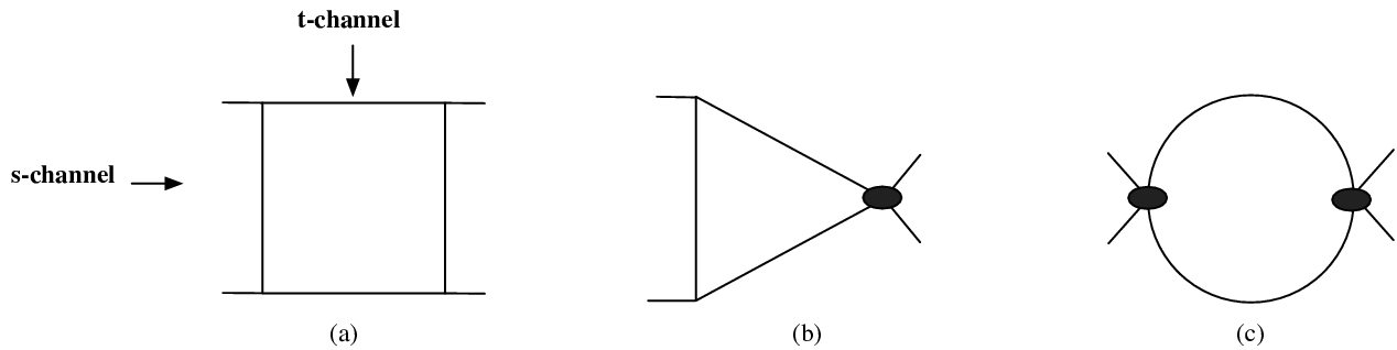
Figure 2: Degeneration limits of the genus-one string amplitude. (a) The limit in which all internal legs are massless propagators. This is the limit that gives the one-loop ten-dimensional supergravity contribution. (b) The triangle limit, in which there are three internal massless propagators. (c) The bubble limit in which two massless propagators are picked out. The blobs in (a) and (b) represent higher derivative contact interactions induced by stringy corrections.

The singularities due to massless two-particle thresholds arise at genus one from the degeneration of the torus in the limit τ2→∞\tau_{2}\to\infty. As indicated in figure 2(a), the zeroth order contribution is simply the type II supergravity box diagram with massless states in all four internal lines, where the threshold behaviour of the S-matrix has the form a1α′slog(−α′s/μ1)R4a_{1}\,{\alpha^{\prime}}\,s\,\log(-\alpha^{\prime}\,s/\mu_{1})\,\textbf{R}^{4}. The constant μ1\mu_{1} cancels out using s+t+u=0s+t+u=0. Figure 2(b) shows the discontinuity receives higher derivative corrections on one side of the cut, due to R4\textbf{R}^{4}, s3​R4s^{3}\,\textbf{R}^{4}, and higher-order contact interactions indicated by the blob. These correspond to threshold terms of the form α′4s4log(−α′s/μ4){\alpha^{\prime}}^{4}\,s^{4}\,\log(-\alpha^{\prime}\,s/\mu_{4}), α′6s6log(−α′s/μ6){\alpha^{\prime}}^{6}\,s^{6}\,\log(-\alpha^{\prime}\,s/\mu_{6}), α′7s7log(−α′s/μ7){\alpha^{\prime}}^{7}\,s^{7}\,\log(-\alpha^{\prime}\,s/\mu_{7}), …\dots. There are also corrections with higher-order contributions on both sides of the cut, as seen in figure 2(c). These lead to higher-order threshold terms.

An important and well-known technical problem in the analysis of these threshold contributions is that the integral representation (1.2) is not well defined for any values of the Mandelstam invariants since the branch points in the ss, tt and uu channels coincide. This is remedied by splitting the integration range of the vertex operator insertion points into three regions 𝒯s​t{\cal T}_{st}, 𝒯u​s{\cal T}_{us} and 𝒯t​u{\cal T}_{tu}, that generate cuts in the (s,t)(s,t), the (s,u)(s,u) and (t,u)(t,u) channels, respectively. The integrand in the 𝒯s​t{\cal T}_{st} region is real for s,t<0s,t<0 (so that u>0u>0) and may be defined in the physical ss-channel region (s>0s>0, t<0t<0) by analytic continuation. Similarly, in the 𝒯u​s{\cal T}_{us} region the integrand is defined for s,u<0s,u<0, while in the 𝒯t​u{\cal T}_{tu} region it is defined for t,u<0t,u<0. Further discussion of the integral representation of the genus-one expression may be found in [10].

4.2.1 The massless supergravity amplitude

In the limit τ2→∞\tau_{2}\to\infty the leading contribution in the 𝒯s​t{\cal T}_{st} region is given by the integral [8]

I𝒯s​t=∫L∞d​τ2τ22​∫𝒯s​t∏i=13d​ωi​eα′​π​τ2​Q​(s,t),I_{{\cal T}_{st}}=\int_{L}^{\infty}{d\tau_{2}\over\tau_{2}^{2}}\,\int_{{\cal T}_{st}}\prod_{i=1}^{3}d\omega_{i}\,e^{\alpha^{\prime}\pi\tau_{2}\,Q(s,t)}\ , (4.16)

where 𝒯s​t={0≤ω1≤ω2≤ω3≤1}{\cal T}_{st}=\{0\leq\omega_{1}\leq\omega_{2}\leq\omega_{3}\leq 1\}, with ωi=ν2(i)/τ2\omega_{i}=\nu_{2}^{(i)}/\tau_{2}. The expression for Q⁡(s,t)Q(s,t)

Q⁡(s,t)=s​ω1​(ω3−ω2)+t⁡(ω2−ω1)​(1−ω3),Q(s,t)=s\omega_{1}(\omega_{3}-\omega_{2})+t(\omega_{2}-\omega_{1})(1-\omega_{3})\,, (4.17)

arises by taking the asymptotic limit of the propagators, limτ2→∞Δs≡Δs∞=𝒫^∞​(ν(12))+𝒫^∞​(ν(34))\lim_{\tau_{2}\to\infty}\Delta_{s}\equiv\Delta^{\infty}_{s}=\hat{\cal P}^{\infty}(\nu^{(12)})+\hat{\cal P}^{\infty}(\nu^{(34)}), in the expression (2.1) for the one-loop amplitude (with ss and tt negative). We need to add the contribution to the amplitude in the regions 𝒯u​s={0≤ω2≤ω1≤ω3≤1}{\cal T}_{us}=\{0\leq\omega_{2}\leq\omega_{1}\leq\omega_{3}\leq 1\} with Q⁡(s,u)=s⁡(ω3−ω1)​ω2+u⁡(ω1−ω2)​(1−ω3)Q(s,u)=s(\omega_{3}-\omega_{1})\omega_{2}+u(\omega_{1}-\omega_{2})(1-\omega_{3}) and 𝒯t​u={0≤ω1≤ω3≤ω2≤1}{\cal T}_{tu}=\{0\leq\omega_{1}\leq\omega_{3}\leq\omega_{2}\leq 1\} with Q⁡(t,u)=u⁡(ω2−ω1)​ω1+t⁡(ω3−ω1)​(1−ω2)Q(t,u)=u(\omega_{2}-\omega_{1})\omega_{1}+t(\omega_{3}-\omega_{1})(1-\omega_{2}). This is equivalent to evaluating the sum of the supergravity box diagrams figure 2(a) in the (s,t)(s,t), (s,u)(s,u) and (t,u)(t,u) channels.

It is very complicated to evaluate the detailed form of this term using the cutoff at τ2≥L\tau_{2}\geq L, so we will review the method used in [11] for evaluating the integral using dimensional regularization. This will generally give a different definition of the scale, μ1\mu_{1}, in terms of the form slog(−α′s/μ1)s\,\log(-\alpha^{\prime}\,s/\mu_{1}). However, in this case the scale cancels out (using s+t+u=0s+t+u=0) and so the result is identical. In D−2​ϵD-2\epsilon dimensions, the one-loop amplitude becomes44 4 We have made use of the change of variables w1=η​ξ1w_{1}=\eta\xi_{1}, w2=(1−η)​(1−ξ2)+η​ξ1w_{2}=(1-\eta)(1-\xi_{2})+\eta\xi_{1} and w3=1−η+η​ξ1w_{3}=1-\eta+\eta\xi_{1}.

I𝒯s​t(d=D−2​ϵ)​(s,t)\displaystyle I_{{\cal T}_{st}}^{(d=D-2\epsilon)}(s,t) =\displaystyle= c⁡(D,ϵ)​∫01d​ξ​(−α′​s​ξ)D2−ϵ−3−(−α′​t​(1−ξ))D2−ϵ−3α′​t+α′​u​ξ,\displaystyle c(D,\epsilon)\,\int_{0}^{1}d\xi\,{(-\alpha^{\prime}s\xi)^{{D\over 2}-\epsilon-3}-(-\alpha^{\prime}t(1-\xi))^{{D\over 2}-\epsilon-3}\over\alpha^{\prime}t+\alpha^{\prime}u\xi}\,, (4.18)

where

c⁡(D,ϵ)=πD2−4−ϵ​Γ⁡(4−D2+ϵ)​Γ​(D2−2−ϵ)2(D−6−2​ϵ)​Γ​(D−4−2​ϵ).c(D,\epsilon)=\pi^{{D\over 2}-4-\epsilon}\,{\Gamma(4-{D\over 2}+\epsilon)\Gamma({D\over 2}-2-\epsilon)^{2}\over(D-6-2\epsilon)\Gamma(D-4-2\epsilon)}\ . (4.19)

In order to perform the ϵ\epsilon expansion we separate the integral into the two contributions

I𝒯s​t(d=D−2​ϵ)​(s,t)=Ks​(s,t)−Kt​(s,t),I_{{\cal T}_{st}}^{(d=D-2\epsilon)}(s,t)=K_{s}(s,t)-K_{t}(s,t)\,, (4.20)

where

Ks​(s,t)=c⁡(D,ϵ)​∫01d​ξ​(−α′​s​ξ)D2−ϵ−3−(−α′​s​ξ∗)D2−ϵ−3α′​t−α′​(s+t)​ξK_{s}(s,t)=c(D,\epsilon)\,\int_{0}^{1}d\xi\,{(-\alpha^{\prime}s\xi)^{{D\over 2}-\epsilon-3}-(-\alpha^{\prime}s\xi_{*})^{{D\over 2}-\epsilon-3}\over\alpha^{\prime}t-\alpha^{\prime}(s+t)\xi} (4.21)

with ξ∗=t/(s+t)\xi_{*}=t/(s+t). In this manner it is clear that the integral over ξ\xi does not develop a singularity in the limit ϵ→0\epsilon\to 0 as long as D>4D>4. In such dimensions ϵ\epsilon singularities can only arise from the factor c⁡(D,ϵ)c(D,\epsilon). These correspond to ultraviolet divergences that first arise as a ϵ\epsilon pole in ten dimensions, c(10,ϵ)→−π/(5!ϵ)c(10,\epsilon)\to-\pi/(5!\,\epsilon) as ϵ→0\epsilon\to 0. For D≤4D\leq 4 the integral may diverge at the ξ=0\xi=0 endpoint, leading to infrared divergences that are seen as singularities in the ϵ→0\epsilon\to 0 limit. We now consider the ten and nine dimensional cases separately.

  • •

    In ten dimensions we have

I𝒯s​t(d=10−2​ϵ)​(s,t)\displaystyle I_{{\cal T}_{st}}^{(d=10-2\epsilon)}(s,t) =\displaystyle= −15!​ϵ​π1−ϵ​e−γE​ϵ​(1+4615​ϵ+O⁡(ϵ2))​(α′​u2−ϵ​I(1)+O⁡(ϵ2))\displaystyle-{1\over 5!\,\epsilon}\,\pi^{1-\epsilon}\,e^{-\gamma_{E}\epsilon}\left(1+{46\over 15}\,\epsilon+O(\epsilon^{2})\right)\,\left({\alpha^{\prime}u\over 2}-\epsilon I^{(1)}+O(\epsilon^{2})\right) (4.22)
=\displaystyle= −α′​u​π240​ϵ+1240​α′​u​π​(γE+log⁡π−4615)+π5!​I𝒯s​t(d=10)​(s,t)+O⁡(ϵ2),\displaystyle-{\alpha^{\prime}u\pi\over 240\,\epsilon}+{1\over 240}\alpha^{\prime}u\,\pi\,(\gamma_{E}+\log\pi-{46\over 15})+{\pi\over 5!}I_{{\cal T}_{st}}^{(d=10)}(s,t)+O(\epsilon^{2})\,,

where γE\gamma_{E} is Euler’s constant. The full result is given by adding the (s,t)(s,t), (t,u)(t,u) and (s,u)(s,u) contributions and using the on-shell condition. The pole in ϵ\epsilon cancels in the sum, leaving the ultraviolet finite result for the full amplitude in the ϵ→0\epsilon\to 0 limit,

IS​U​G​R​A(d=10)​(s,t,u)=I𝒯s​t(d=10)​(s,t)+I𝒯t​u(d=10)​(t,u)+I𝒯u​s(d=10)​(u,s),I_{SUGRA}^{(d=10)}(s,t,u)=I_{{\cal T}_{st}}^{(d=10)}(s,t)+I_{{\cal T}_{tu}}^{(d=10)}(t,u)+I_{{\cal T}_{us}}^{(d=10)}(u,s)\,, (4.23)

where the function I𝒯s​t(d=10)I_{{\cal T}_{st}}^{(d=10)} is given by

I𝒯s​t(d=10)​(s,t)\displaystyle I_{{\cal T}_{st}}^{(d=10)}(s,t) =\displaystyle= ∫01d​ξα′​t+α′​u​ξ​[(−α′​t​(1−ξ))2​log⁡(−α′​t​(1−ξ))−(−α′​s​ξ)2​log⁡(−α′​s​ξ)].\displaystyle\int_{0}^{1}{d\xi\over\alpha^{\prime}t+\alpha^{\prime}u\xi}\,\left[(-\alpha^{\prime}t(1-\xi))^{2}\log(-\alpha^{\prime}t(1-\xi))-(-\alpha^{\prime}s\xi)^{2}\log(-\alpha^{\prime}s\xi)\right]\,.

This expression is real in the region s<0s<0, t<0t<0 and has the appropriate imaginary part in other regions of the Mandelstam invariants. For example, in the physical region, s>0s>0 and t,u<0t,u<0, the integrand in () is nonsingular in the whole range of ξ\xi, so the only singularities are branch points due to the explicit log⁡(−α′​s)\log(-\alpha^{\prime}s) factor. The pole of the denominator at ξ=−t/u\xi=-t/u is canceled by a zero in the numerator and the integrand is finite in the range of integration, as is evident from the form of Ks​(s,t)K_{s}(s,t) in (4.21). Other singularities with double discontinuities can be found by analytic continuation.

Evaluating the integrals in () explicitly leads to

I𝒯s​t(d=10)​(s,t)\displaystyle I^{(d=10)}_{{\cal T}_{st}}(s,t) =\displaystyle= α′​u4+α′​s​t2​u+α′​s2​(s+3​t)​log⁡(−α′​s)+t2​(t+3​s)​log⁡(−α′​t)2​u2\displaystyle{\alpha^{\prime}u\over 4}+\alpha^{\prime}{st\over 2u}+\alpha^{\prime}\,{s^{2}(s+3t)\,\log(-\alpha^{\prime}s)+t^{2}(t+3s)\,\log(-\alpha^{\prime}t)\over 2u^{2}} (4.25)
−α′​s2​t2u3​(ℒ2​(−ut)+ℒ2​(−us)),\displaystyle-\alpha^{\prime}{s^{2}t^{2}\over u^{3}}\left(\mathcal{L}_{2}\left(-{u\over t}\right)+\mathcal{L}_{2}\left(-{u\over s}\right)\right)\,,

where

ℒ2​(x)=Li2​(x)+log⁡(x)​log⁡(1−x)=π26−Li2​(1−x)\mathcal{L}_{2}(x)=\textrm{Li}_{2}(x)+\log(x)\log(1-x)={\pi^{2}\over 6}-\textrm{Li}_{2}(1-x) (4.26)

is a real function for all x≥0x\geq 0 [12]. Although I𝒯s​t(d=10)​(s,t)I_{{\cal T}_{st}}^{(d=10)}(s,t) is a complicated expression it is easy to see that it has the important scaling property

I𝒯s​t(d=10)​(L​s,L​t)=L​I(1)​(s,t)−α′​u2​L​log⁡(L),I_{{\cal T}_{st}}^{(d=10)}(Ls,Lt)=L\,I^{(1)}(s,t)-{\alpha^{\prime}u\over 2}\,L\log(L)\,, (4.27)

which ensures that the scale of the logarithm does not contribute after summation over the (s,t)(s,t), (t,u)(t,u) and (s,u)(s,u) terms.

∙\bullet For completeness, we also include the case of nine dimensions, where there are no divergences when ϵ→0\epsilon\to 0 and we can set ϵ=0\epsilon=0 directly in the expression for the amplitude, giving

I𝒯s​t(d=9)​(s,t)\displaystyle I_{{\cal T}_{st}}^{(d=9)}(s,t) =\displaystyle= 23​(−α′​s)3/2+(−α′​t)3/2α′​u−2​(−α′​s)3/2​t+(−α′​t)3/2​sα′​u2\displaystyle{2\over 3}\,{(-\alpha^{\prime}s)^{3/2}+(-\alpha^{\prime}t)^{3/2}\over\alpha^{\prime}u}-2{(-\alpha^{\prime}s)^{3/2}t+(-\alpha^{\prime}t)^{3/2}s\over\alpha^{\prime}u^{2}} (4.28)
+3​(−α′​s)3/2​(−α′​t)3/2(α′​u)5/2​log⁡((−α′​t+α′​u)​(−α′​s−α′​u)(−α′​t−α′​u)​(−α′​s+α′​u)).\displaystyle+{3(-{\alpha^{\prime}}s)^{3/2}(-\alpha^{\prime}t)^{3/2}\over(\alpha^{\prime}u)^{5/2}}\,\log\left((\sqrt{-\alpha^{\prime}t}+\sqrt{\alpha^{\prime}u})(\sqrt{-\alpha^{\prime}s}-\sqrt{\alpha^{\prime}u})\over(\sqrt{-\alpha^{\prime}t}-\sqrt{\alpha^{\prime}u})(\sqrt{-\alpha^{\prime}s}+\sqrt{\alpha^{\prime}u})\right)\,.

Once again the full expression for In​o​n​a​n(d=19)​(s,t,u)I_{nonan}^{(d=19)}(s,t,u) is obtained by adding the contributions of I𝒯t​u(d=10)I_{{\cal T}_{tu}}^{(d=10)} and I𝒯u​s(d=10)I_{{\cal T}_{us}}^{(d=10)} to I𝒯s​t(d=10)I_{{\cal T}_{st}}^{(d=10)}.

4.2.2 String corrections and higher-order massless thresholds

At higher order in the derivative expansion there are further massless threshold effects due to the higher-order contact terms in the blob in figures 2(b) and 2(c). These lead to factors of the form srlog(−s/μr)s^{r}\,\log(-s/\mu_{r}), where the scale of the logarithm does not cancel. Luckily the threshold structure of these terms is much simpler than that of the box diagram in figure 2(a) since they only possess singularities in ss rather than overlapping singularities. So we can go back to the cutoff procedure outlined earlier in order to evaluate the expressions, taking care to verify that the dependence on the cutoff LL indeed cancels.

The supergravity contribution considered in the last subsection was obtained by replacing the propagators in the exponent of (2.1) by their leading form in the large-τ2\tau_{2} limit. In order to analyze threshold terms at higher-order in the momentum expansion we need to keep non-leading terms at large τ2\tau_{2}. To do this we write

Δs∼Δs∞+δs,\Delta_{s}\sim\Delta_{s}^{\infty}+\delta_{s}\,, (4.29)

where the correction, δs\delta_{s}, to the asymptotic value is given by the k=0k=0 part of P~​(ν|τ){\tilde{P}}(\nu|\tau) defined in (2.16),

δs=∑m≠014​|m|​(e2​i​π​(m​ν1(12)+i​|m​ν2(12)|)+e2​i​π​(m​ν1(34)+i​|m​ν2(34)|)),\delta_{s}=\sum_{m\neq 0}{1\over 4|m|}\,\left(e^{2i\pi(m\nu^{(12)}_{1}+i|m\nu^{(12)}_{2}|)}+e^{2i\pi(m\nu^{(34)}_{1}+i|m\nu^{(34)}_{2}|)}\right)\,, (4.30)

with similar expressions for δt,u\delta_{t,u}. In the τ2≥L\tau_{2}\geq L region the terms with k≠0k\neq 0 are suppressed by powers of e−Le^{-L}. The asymptotic formula for the amplitude is therefore given by [4],

I𝒯s​t;ℛL​(s,t)\displaystyle I_{{\cal T}_{st};{\cal R}_{L}}(s,t) =\displaystyle= ∫L∞d​τ2τ22​∫𝒯s​t∏i=13d2​ντ2​exp⁡(α′​s​(Δs∞−Δu∞)+α′​t​(Δ~t∞−Δ~u∞))\displaystyle\int_{L}^{\infty}{d\tau_{2}\over\tau_{2}^{2}}\,\int_{{\cal T}_{st}}\prod_{i=1}^{3}{d^{2}\nu\over\tau_{2}}\,\exp\left(\alpha^{\prime}s(\Delta^{\infty}_{s}-\Delta^{\infty}_{u})+\alpha^{\prime}t(\tilde{\Delta}^{\infty}_{t}-\tilde{\Delta}^{\infty}_{u})\right) (4.31)
exp⁡(α′​s​(δs−δu)+α′​t​(δt−δu)).\displaystyle\qquad\qquad\qquad\exp\left({\alpha^{\prime}}s(\delta_{s}-\delta_{u})+{\alpha^{\prime}}t(\delta_{t}-\delta_{u})\right)\,.

The higher-order threshold contributions containing factors of log⁡(−s​L)\log(-sL) are obtained by expanding the integrand in powers of δ\delta, eα′​δ=1+α′​δ+α′2​δ2/2+…e^{{\alpha^{\prime}}\delta}=1+{\alpha^{\prime}}\delta+{\alpha^{\prime}}^{2}\delta^{2}/2+\dots. The factors of eα′​Δ∞e^{\alpha^{\prime}\,\Delta^{\infty}} in the integrand contribute to terms with positive powers of LL.

In particular, the terms of order α′4s4log(−α′s/μ4){\alpha^{\prime}}^{4}\,s^{4}\log(-{\alpha^{\prime}}s/\mu_{4}), which will be denoted I(4)I^{(4)}, is obtained from the δs2\delta_{s}^{2} contribution of the integrand in (4.31). Neither δt\delta_{t} or δu\delta_{u} contributes to this threshold behaviour term (although δt\delta_{t} does contribute to the analogous tt-channel term, α′4t4log(−α′t/μ4){\alpha^{\prime}}^{4}\,t^{4}\,\log(-{\alpha^{\prime}}t/\mu_{4})). This gives

I𝒯s​t;ℛL(4)​(s,t)\displaystyle I^{(4)}_{{\cal T}_{st};{\cal R}_{L}}(s,t) =\displaystyle= 12​∑m≠0(−α′​s)2(4​m)2​∫L∞d​τ2τ22​∫𝒯s​t∏i=13d​ωi​eα′​π​τ2​Q​(s,t)−4​π​|m|​τ2​(ω2−ω1)\displaystyle{1\over 2}\sum_{m\neq 0}{(-\alpha^{\prime}s)^{2}\over(4m)^{2}}\int_{L}^{\infty}{d\tau_{2}\over\tau_{2}^{2}}\int_{{\cal T}_{st}}\prod_{i=1}^{3}d\omega_{i}e^{\alpha^{\prime}\pi\tau_{2}Q(s,t)-4\pi|m|\tau_{2}(\omega_{2}-\omega_{1})} (4.32)
+\displaystyle+ 12​∑m≠0(−α′​s)2(4​m)2​∫L∞d​τ2τ22​∫𝒯s​t∏i=13d​ωi​eα′​π​τ2​Q​(s,t)−4​π​|m|​τ2​(1−ω3)\displaystyle{1\over 2}\sum_{m\neq 0}{(-\alpha^{\prime}s)^{2}\over(4m)^{2}}\int_{L}^{\infty}{d\tau_{2}\over\tau_{2}^{2}}\int_{{\cal T}_{st}}\prod_{i=1}^{3}d\omega_{i}e^{\alpha^{\prime}\pi\tau_{2}Q(s,t)-4\pi|m|\tau_{2}(1-\omega_{3})}
=\displaystyle= ∑m≠0(−α′​s)2(4​m)2​g(4)​(L,s,t),\displaystyle\sum_{m\neq 0}\,{(-\alpha^{\prime}s)^{2}\over(4m)^{2}}\,g^{(4)}(L;s,t)\,,

where we note that the two terms on the right-hand side of the first equality are equal and

g(4)​(L,s,t)\displaystyle g^{(4)}(L;s,t) =\displaystyle= ∫L∞d​τ2τ22​∫01d​η​d​ξ1​d​ξ2​η​(1−η)​eα′​π​τ2​Q​(s,t)−4​π​|m|​τ2​(1−ξ2)​(1−η).\displaystyle\int_{L}^{\infty}{d\tau_{2}\over\tau_{2}^{2}}\int_{0}^{1}d\eta\,d\xi_{1}d\xi_{2}\,\eta(1-\eta)\,e^{\alpha^{\prime}\pi\tau_{2}Q(s,t)-4\pi|m|\tau_{2}(1-\xi_{2})(1-\eta)}\,. (4.33)

Noting further that QQ is given in terms of the variables η\eta, ξ1\xi_{1} and ξ2\xi_{2} by

Q⁡(s,t)=s​η​(1−η)​ξ1​ξ2+t​η​(1−η)​(1−ξ1)​(1−ξ2),Q(s,t)=s\,\eta(1-\eta)\,\xi_{1}\,\xi_{2}+t\,\eta(1-\eta)\,(1-\xi_{1})\,(1-\xi_{2})\,, (4.34)

and performing the ξ2\xi_{2} integral gives

g(4)​(L,s,t)\displaystyle g^{(4)}(L;s,t) =\displaystyle= ∫L∞d​τ2τ23​∫01d​η​d​ξ1​η​eα′​π​s​τ2​η​(1−η)​ξ1−e−4​π​m​τ2​(1−η)​eα′​π​t​τ2​η​(1−η)​(1−ξ1)α′​η​π​(s​ξ1−t⁡(1−ξ1))+4​π​m.\displaystyle\int_{L}^{\infty}{d\tau_{2}\over\tau_{2}^{3}}\int_{0}^{1}d\eta\,d\xi_{1}\,\eta\,{e^{{\alpha^{\prime}}\pi s\tau_{2}\eta(1-\eta)\xi_{1}}-e^{-4\pi m\tau_{2}(1-\eta)}e^{{\alpha^{\prime}}\pi t\tau_{2}\eta(1-\eta)(1-\xi_{1})}\over{\alpha^{\prime}}\eta\pi(s\xi_{1}-t(1-\xi_{1}))+4\pi m}\,. (4.35)

The term of order s4s^{4} in the amplitude comes from the O⁡(α′3)O({\alpha^{\prime}}^{3}) correction to the tree amplitude represented by the blob in 2(b). This is obtained by expanding g(4)g^{(4)} to O⁡(s2)O(s^{2}). At this order it is easy to see that the term proportional to e−4​π​m​τ2​(1−η)e^{-4\pi m\tau_{2}(1-\eta)} in the numerator of (4.35) is proportional to e−Le^{-L} and is negligible. The term of the form s2​log⁡(−α′​s)s^{2}\log(-\alpha^{\prime}\,s) arises by expanding eα′​π​s​τ2​η​(1−η)​ξ1e^{{\alpha^{\prime}}\pi s\tau_{2}\eta(1-\eta)\xi_{1}} to quadratic order and replacing the denominator by 4​π​m4\pi m. As a result we find the O⁡(s2)O(s^{2}) terms,

g(4)(L;s,t)=−14​π​m(α′​s​π)2180(log(−α′sπL/ce)−2/5)L3+O(s3,L−1),g^{(4)}(L;s,t)=-{1\over 4\pi m}\,{(\alpha^{\prime}s\,\pi)^{2}\over 180}\,\left(\log(-\alpha^{\prime}s\,\pi\,L/c_{e})-2/5\right)L^{3}+O(s^{3},L^{-1})\,, (4.36)

where ce=exp⁡(−γE)c_{e}=\exp(-\gamma_{E}). In obtaining this we have used the fact that

limx→0∫L∞d​tt3​e−x​t=12​L2−xL−x22​(log⁡(x​L)−3/2+γ)+o⁡(x2).\lim_{x\to 0}\int_{L}^{\infty}\frac{dt}{t^{3}}\,e^{-xt}=\frac{1}{2L^{2}}-\frac{x}{L}-\frac{x^{2}}{2}\left(\log(xL)-3/2+\gamma\right)+o(x^{2}). (4.37)

Substituting (4.36) into (4.32) gives the contribution

I𝒯s​t;ℛL(4)​(s,t)\displaystyle I^{(4)}_{{\cal T}_{st};{\cal R}_{L}}(s,t) =\displaystyle= −2​π​ζ​(3)45(α′4)4s4log(−α′sL/μ^4)+⋯,\displaystyle-{2\pi\zeta(3)\over 45}\,\left(\frac{\alpha^{\prime}}{4}\right)^{4}\,s^{4}\log(-\alpha^{\prime}s\,L/\hat{\mu}_{4})+\cdots\,, (4.38)

where the scale of the logarithm at this order is given by

log⁡μ^4=25−log⁡(π/ce).\log\hat{\mu}_{4}={2\over 5}-\log(\pi/c_{e})\ . (4.39)

The ellipses indicate that a similar contribution that arises by using the δt2\delta_{t}^{2} term in the expansion of eα′​t​δte^{{\alpha^{\prime}}t\delta_{t}}, which gives a threshold singularity in the tt channel in which figure 2(b) is transformed by interchanging ss and tt. There are similarly contributions from 𝒯u​s{\cal T}_{us} and 𝒯t​u{\cal T}_{tu} regions containing analogous terms with ss, tt and uu-channel thresholds.

Therefore the total contribution from the upper part of the fundamental domain τ2≥L\tau_{2}\geq L to the terms of order s4s^{4} is given by the sum

IℛL(4)​(s,t,u)=I𝒯s​t;ℛL(4)​(s,t)+I𝒯t​u;ℛL(4)​(t,u)+I𝒯u​s;ℛL(4)​(u,s)=−4​ζ​(3)45​π(α′4)4s4log(−α′sLπ/ce)−2/5)+(s→t)+(s→u).\begin{split}&I^{(4)}_{{\cal R}_{L}}(s,t,u)=I^{(4)}_{{\cal T}_{st};{\cal R}_{L}}(s,t)+I^{(4)}_{{\cal T}_{tu};{\cal R}_{L}}(t,u)+I^{(4)}_{{\cal T}_{us};{\cal R}_{L}}(u,s)\\ &=-{4\zeta(3)\over 45\pi}\left(\frac{\alpha^{\prime}}{4}\right)^{4}\,s^{4}\,\log(-\alpha^{\prime}sL\pi/c_{e})-2/5)+(s\to t)+(s\to u)\,.\end{split} (4.40)

The dependence on both L3L^{3} and log⁡(L)\log(L) cancel in the sum of this contribution and the contribution from τ2≤L\tau_{2}\leq L given in (3.17), giving

In​o​n​a​n(4)​(s,t,u)=−4​π​ζ​(3)45(α′4)4[s4log(−α′s/μ4)+t4log(−α′t/μ4)+u4log(−α′u/μ4)−6/5],\begin{split}I^{(4)}_{nonan}(s,t,u)&=-{4\pi\zeta(3)\over 45}\,\left(\frac{\alpha^{\prime}}{4}\right)^{4}\left[s^{4}\,\log(-\alpha^{\prime}s/\mu_{4})\right.\\ &\left.+t^{4}\,\log(-\alpha^{\prime}t/\mu_{4})+u^{4}\,\log(-\alpha^{\prime}u/\mu_{4})-6/5\right]\,,\end{split} (4.41)

where

log⁡μ4=log⁡μ^4−log⁡μ~4=910−log⁡(2π​ce)+ζ′​(3)ζ⁡(3)−ζ′​(4)ζ⁡(4),\log\mu_{4}=\log\hat{\mu}_{4}-\log\tilde{\mu}_{4}={9\over 10}-\log\left({2\over\pi c_{e}}\right)+{\zeta^{\prime}(3)\over\zeta(3)}-{\zeta^{\prime}(4)\over\zeta(4)}\,, (4.42)

which is the sum of the scale from the lower part of the fundamental domain, given in (3.18), and the scale in the logarithm obtained from the above computation from the large-τ2\tau_{2} part of the fundamental domain (4.39).

Contributions to terms of order s5s^{5} arise both from expanding the function g(4)​(L,s,t)g^{(4)}(L;s,t) to one further order in ss and by bringing down one further power of δ\delta from the exponential in (4.31). In this case the there are no terms proportional to log⁡L\log L, which reflects the fact that there is no threshold term at this order, as follows from the unitarity argument in section 4.1. In order to evaluate the thresholds at order α′6s6log(−α′s/μ6){\alpha^{\prime}}^{6}\,s^{6}\log(-{\alpha^{\prime}}s/\mu_{6}), it is necessary to expand g(4)​(L,s,t)g^{(4)}(L;s,t) to two further orders in ss, which is fairly complicated. In addition, there are contributions from yet higher powers of δ\delta. Although we have not evaluated these terms, in principle, they will determine a scale log⁡μ^6\log\hat{\mu}_{6} (analogous to log⁡μ^4\log\hat{\mu}_{4} in (4.39)) that combines with log⁡μ~6\log\tilde{\mu}_{6} (3.27) to give the scale log⁡μ6\log\mu_{6}.

At higher orders in α′\alpha^{\prime} string corrections arise on both sides of the threshold discontinuity as we saw in section 4.1. The qualitative structure of these threshold contributions matches that of the discontinuities that we determined earlier from unitarity. Firstly, there are contributions from the triangle diagram in figure 2(b) beyond the ones considered above. The first of these is of order α′​s7​log⁡(−α′​s)\alpha^{\prime}\,s^{7}\log(-\alpha^{\prime}\,s). In addition, a new class of contributions arises, in which both the propagators on the left and right of the ss-channel cut are canceled and the result is the diagram in figure 2(c), which has two blobs representing the higher derivative vertices.

4.3 Summary of the expansion of the ten-dimensional genus-one amplitude

To put these results in perspective we will here summarize the low-energy expansion of the genus-one contribution to the analytic part of the amplitude up to order s6​R4s^{6}\,\textbf{R}^{4}. At tree-level and genus one, type IIA and type IIB massless four-particle amplitudes are completely equivalent, so the results apply equally to both cases.

The analytic terms to this order are summarized by

Aa​ng​e​n​u​s−1​(σ^2,σ^3)\displaystyle\textbf{A}^{genus-1}_{an}(\hat{\sigma}_{2},\hat{\sigma}_{3}) =\displaystyle= π3​(∑p,qJ(p,q)​σ^2p​σ^3q)​R4\displaystyle{\pi\over 3}\,\left(\sum_{p,q}J^{(p,q)}\,\hat{\sigma}_{2}^{p}\hat{\sigma}_{3}^{q}\right)\,\textbf{R}^{4} (4.43)
=\displaystyle= π3​(1+0​σ^2+ζ⁡(3)3​σ^3+0​σ^22+971080​ζ​(5)​σ^2​σ^3CLOSE\displaystyle{\pi\over 3}\,\left(1+0\,\hat{\sigma}_{2}+{\zeta(3)\over 3}\hat{\sigma}_{3}+0\,\hat{\sigma}_{2}^{2}+{97\over 1080}\,\zeta(5)\,\hat{\sigma}_{2}\hat{\sigma}_{3}\right.
OPEN+130​ζ​(3)2​σ^23+611080​ζ​(3)2​σ^32+⋯)​R4,\displaystyle\qquad\quad\left.+{1\over 30}\,\zeta(3)^{2}\hat{\sigma}_{2}^{3}+{61\over 1080}\zeta(3)^{2}\hat{\sigma}_{3}^{2}+\cdots\right)\,\textbf{R}^{4}\,,

(where we have indicated explicitly the vanishing σ^2\hat{\sigma}_{2} and σ^22\hat{\sigma}_{2}^{2} coefficients), while the nonanalytic terms are contained in

An​o​n​a​ng​e​n​u​s−1​(σ^2,σ^3)=AS​U​G​R​Ag​e​n​u​s−1+(α′4)4​4​ζ​(3)​π45​(s4​log⁡(−α′​sμ4)+t4​log⁡(−α′​tμ4)+u4​log⁡(−α′​uμ4))​R4+(α′4)6​π​ζ​(5)2520​((87​s6+s4​(t−u)2)​log⁡(−α′​sμ6)CLOSEOPEN+(87​t6+t4​(s−u)2)​log⁡(−α′​tμ6)+(87​u6+u4​(s−t)2)​log⁡(−α′​uμ6))​R4+⋯,\begin{split}\textbf{A}^{genus-1}_{nonan}(\hat{\sigma}_{2},\hat{\sigma}_{3})&=\textbf{A}^{genus-1}_{SUGRA}\\ &+\left(\frac{\alpha^{\prime}}{4}\right)^{4}{4\zeta(3)\pi\over 45}\,\Big(s^{4}\,\log(-{\alpha^{\prime}\,s\over\mu_{4}})+t^{4}\,\log(-{\alpha^{\prime}\,t\over\mu_{4}})+u^{4}\,\log(-{\alpha^{\prime}\,u\over\mu_{4}})\Big)\,\textbf{R}^{4}\\ &+\left(\frac{\alpha^{\prime}}{4}\right)^{6}{\pi\,\zeta(5)\over 2520}\,\Big((87\,s^{6}+s^{4}\,(t-u)^{2})\,\log(-{\alpha^{\prime}\,s\over\mu_{6}})\\ &+(87\,t^{6}+t^{4}\,(s-u)^{2})\,\log(-{\alpha^{\prime}\,t\over\mu_{6}})+(87\,u^{6}+u^{4}\,(s-t)^{2})\,\log(-{\alpha^{\prime}\,u\over\mu_{6}})\Big)\,\textbf{R}^{4}+\cdots\,,\end{split} (4.44)

where AS​U​G​R​Ag​e​n​u​s−1\textbf{A}^{genus-1}_{SUGRA} is the result obtained in ten-dimensional maximal supergravity that we described earlier where we also discussed the scales μ4\mu_{4} and μ6\mu_{6}. Notice that the terms in equations (4.43) and (4.44) satisfy a ‘transcendentality condition’ in which ζ⁡(k)\zeta(k) is associated with a weight kk, π\pi has weight 1 and log⁡(x)\log(x) also has weight 11. The total weight of a term of order (α′)q({\alpha^{\prime}})^{q} is q+1q+1.

Clearly, the separation of the amplitude into Aa​n\textbf{A}_{an} and An​o​n​a​n\textbf{A}_{nonan} depends on the definition of the scales inside the logarithmic terms in (4.44). The sum of the terms that depend on μ4\mu_{4} and μ6\mu_{6} is

−4​π​ζ​(3)45​σ^22​log⁡μ4​R4−ζ⁡(5)​π630​(11​σ^23+14​σ^32)​log⁡μ6​R4.-\frac{4\pi\zeta(3)}{45}\,\hat{\sigma}_{2}^{2}\,\log\mu_{4}\,\textbf{R}^{4}-{\zeta(5)\pi\over 630}\,\left(11\hat{\sigma}_{2}^{3}+14\hat{\sigma}_{3}^{2}\right)\,\log\mu_{6}\,\textbf{R}^{4}\,. (4.45)

Notice that although changing the scale inside the logarithms alters the analytic part of the amplitude, the pattern of Riemann zeta values is different in the coefficients of the terms in Aa​ng​e​n​u​s−1\textbf{A}^{genus-1}_{an} from those in An​o​n​a​ng​e​n​u​s−1\textbf{A}^{genus-1}_{nonan}. In this sense, there is an objective meaning to the separation between the analytic and the nonanalytic parts as given in (4.43) and (4.44). For example, at order (α′​s)6(\alpha^{\prime}\,s)^{6} one has a finite piece proportional to ζ​(3)2\zeta(3)^{2} while the logarithmic term is multiplied by ζ⁡(5)\zeta(5) in agreement with the ‘transcendentality’ property noted earlier. So our choice of scale in the argument of the logarithmic terms is not only the natural scale that arises from the calculation of section 3, but is natural if ζ​(3)2\zeta(3)^{2} and ζ⁡(5)\zeta(5) are considered to be distinct coefficients.

5 The genus-one four-particle amplitude in nine dimensions

We now turn to consider the compactification of the amplitude on a circle of radius rr so that nine-space-time dimensions are non-compact. We will specialize to the case in which the momenta of the scattering particles, prμp_{r}^{\mu}, have zero components in the compact direction, so the external states are Kaluza–Klein ground states. In nine dimensions the genus-one normal thresholds have square root singularities instead of logarithms. This separates the threshold terms in the amplitude from the analytic terms in a very clear manner. The massive Kaluza–Klein modes also generate massive square root thresholds that are expanded, when α′​s≫1/r2\alpha^{\prime}s\gg 1/r^{2}, in an infinite series of terms of the form (α′​s​r2)n(\alpha^{\prime}sr^{2})^{n} and therefore enter into higher order terms in the low energy expansion. The logarithmic singularities characteristic of ten dimensions are recovered in the ten-dimensional limit by a condensation of these Kaluza–Klein thresholds [7].

5.1 General method

The expression for the integral II in the compactified genus-one amplitude (1.1) now has the form

I(d=9)​(s,t,u,r)=∫ℱd2​ττ22​τ2​Γ(1,1)​(r)​F​(s,t,u,τ),I^{(d=9)}(s,t,u;r)=\int_{{\cal F}}{d^{2}\tau\over\tau_{2}^{2}}\,\sqrt{\tau_{2}}\ \Gamma_{(1,1)}(r)\,F(s,t,u;\tau)\,, (5.1)

where the lattice sum factor is given by [11]

τ2​Γ(1,1)​(r)=τ2​∑(m,n^)∈ℤ2e−π​τ2​((mr)2+(n^​r)2)+2​i​π​τ1​m^​n.\sqrt{\tau_{2}}\ \Gamma_{(1,1)}(r)=\sqrt{\tau_{2}}\sum_{(m,\hat{n})\in{\mathbb{Z}}^{2}}\,e^{-\pi\tau_{2}\left((\frac{m}{r})^{2}+(\hat{n}r)^{2}\right)+2i\pi\tau_{1}{\hat{m}}n}\,. (5.2)

The loop amplitude can now be expressed in terms of an expansion in half-integer powers of α′​s\alpha^{\prime}s, α′​t\alpha^{\prime}t and α′​u\alpha^{\prime}u. We can separate this into two terms,

I(d=9)​(s,t,u,r)=Ia​n(d=9)​(s,t,u,r)+In​o​n​a​n(d=9)​(s,t,u,r).I^{(d=9)}(s,t,u;r)=I_{an}^{(d=9)}(s,t,u;r)+I_{nonan}^{(d=9)}(s,t,u;r)\,. (5.3)

The analytic part has an expansion with integer powers of the Mandelstam invariants of the form

Ia​n(d=9)​(s,t,u,r)=∑p,q=0∞J(p,q)​(r)​σ^2p​σ^3qI_{an}^{(d=9)}(s,t,u;r)=\sum_{p,q=0}^{\infty}J^{(p,q)}(r)\,\hat{\sigma}_{2}^{p}\hat{\sigma}_{3}^{q} (5.4)

and is analytic in ss, tt and uu. We will see that the coefficients can be expanded at large rr as sums of powers of rr, together with r​log⁡r2r\log r^{2} terms and exponentials,

J(p,q)​(r)\displaystyle J^{(p,q)}(r) =\displaystyle= J1(p,q)​r4​p+6​q−1+J2(p,q)​r4​p+6​q−3+⋯+J4​p+6​q(p,q)​r−4​p−6​q+1\displaystyle J^{(p,q)}_{1}\,r^{4p+6q-1}+J^{(p,q)}_{2}\,r^{4p+6q-3}+\dots+J^{(p,q)}_{4p+6q}\,r^{-4p-6q+1} (5.5)
+K(p,q)​r​log⁡(r2​λ2​p+3​q)+O⁡(e−r),\displaystyle+K^{(p,q)}\,r\log(r^{2}\lambda_{2p+3q})+O(e^{-r})\,,

where the λk\lambda_{k}’s are constants. In the ten-dimensional theory only the term linear in rr survives with coefficient J2​p+3​q(p,q)J^{(p,q)}_{2p+3q}. The nonanalytic part has the form

In​o​n​a​n(d=9)​(s,t,u,r)=b1​s12+b4​s72+⋯,I_{nonan}^{(d=9)}(s,t,u;r)=b_{1}s^{{\scriptstyle{1\over 2}}}+b_{4}s^{{\scriptstyle{7\over 2}}}+\cdots\,, (5.6)

where terms involving tt and uu have not been included. The coefficients bib_{i} are independent of rr. In the following we will be interested in determining the coefficients Jr(p,q)J^{(p,q)}_{r} in the expansion of Ia​n(d=9)I^{(d=9)}_{an}, but will not consider the coefficients bnb_{n} of the non-analytic terms in any detail (although they are relatively easy to extract).

We will first reexpress the lattice sum by a Poisson resummation that replaces the sum over mm by a sum over p^\hat{p} and two relatively prime integers (m^,n^)(\hat{m},\hat{n}),

τ2​∑(m,n^)∈ℤ2e−π​τ2​((mr)2+(n^​r)2)+2​i​π​τ1​m​n^=r​∑p^∈ℤ(m^,n^)=1e−π​p^2​r2​|m^+n^​τ|2τ2.\sqrt{\tau_{2}}\sum_{(m,\hat{n})\in{\mathbb{Z}}^{2}}\,e^{-\pi\tau_{2}\left((\frac{m}{r})^{2}+(\hat{n}r)^{2}\right)+2i\pi\tau_{1}{m\hat{n}}}=r\,\sum_{\hat{p}\in{\mathbb{Z}}\atop(\hat{m},\hat{n})=1}\,e^{-\pi\,\hat{p}^{2}\,r^{2}\,{|\hat{m}+\hat{n}\tau|^{2}\over\tau_{2}}}\,. (5.7)

Thanks to the modular invariance of the kinematical factor F⁡(s,t,u,τ)F(s,t,u;\tau), after separating the zero-winding term (p^=0\hat{p}=0) one can unfold the integral onto the semi-infinite strip [6], which gives

I(d=9)​(s,t,u,r)\displaystyle I^{(d=9)}(s,t,u;r) =\displaystyle= r​∫ℱd2​ττ22​F​(s,t,u,τ)\displaystyle r\,\int_{{\cal F}}{d^{2}\tau\over\tau_{2}^{2}}\,F(s,t,u;\tau) (5.8)
+\displaystyle+ r​∑p^≠0∫0∞d​τ2τ22​e−π​p^2​r2τ2​∫−1212d​τ1​F​(s,t,u,τ).\displaystyle r\,\sum_{\hat{p}\neq 0}\int_{0}^{\infty}{d\tau_{2}\over\tau_{2}^{2}}\,e^{-\pi\hat{p}^{2}\frac{r^{2}}{\tau_{2}}}\int_{-{\scriptstyle{1\over 2}}}^{{\scriptstyle{1\over 2}}}d\tau_{1}\,F(s,t,u;\tau)\,\,.

The first term is the zero-winding term, which is the term that survives the r→∞r\to\infty limit,

r​∫ℱd2​ττ22​F​(s,t,u,τ)=r​I(d=10)​(s,t,u),r\,\int_{{\cal F}}{d^{2}\tau\over\tau_{2}^{2}}\,\,F(s,t,u;\tau)=r\,I^{(d=10)}(s,t,u)\,, (5.9)

where the low-energy expansion of I(d=10)​(s,t,u)I^{(d=10)}(s,t,u) was considered in sections 3 and 4.

Proceeding as for the ten-dimensional amplitude in section 3, the integral Ip^≠0(d=9)I^{(d=9)}_{\hat{p}\neq 0} can be split into an analytic and non-analytic parts by dividing the τ2\tau_{2} integral into two domains, so that I(d=9)=I(1)(d=9)+I(2)(d=9)I^{(d=9)}=I^{(d=9)}_{(1)}+I^{(d=9)}_{(2)}, where

I(1)(d=9)=r​∑p^≠0∫0Ld​τ2τ22​e−π​p^2​r2τ2​∫−1212d​τ1​F​(s,t,u,τ)I^{(d=9)}_{(1)}=r\,\sum_{\hat{p}\neq 0}\int_{0}^{L}{d\tau_{2}\over\tau_{2}^{2}}\,e^{-\pi\hat{p}^{2}\frac{r^{2}}{\tau_{2}}}\,\int_{-{\scriptstyle{1\over 2}}}^{{\scriptstyle{1\over 2}}}d\tau_{1}\,F(s,t,u;\tau)\, (5.10)

contains the analytic part of the amplitude, and

I(2)(d=9)=r​∑p^≠0∫L∞d​τ2τ22​e−π​p^2​r2τ2​∫−1212d​τ1​F​(s,t,u,τ),I^{(d=9)}_{(2)}=r\,\sum_{\hat{p}\neq 0}\int_{L}^{\infty}{d\tau_{2}\over\tau_{2}^{2}}\,e^{-\pi\hat{p}^{2}\frac{r^{2}}{\tau_{2}}}\,\int_{-{\scriptstyle{1\over 2}}}^{{\scriptstyle{1\over 2}}}d\tau_{1}\,F(s,t,u;\tau)\,, (5.11)

contains the non-analytic threshold terms. As in the ten-dimensional case, the LL dependence will cancel from the final expressions.

The analytic contributions in equation (5.10) can be analyzed by expanding ∫d​τ1​F​(s,t,u,τ)\int d\tau_{1}F(s,t,u;\tau) in powers of σ^2\hat{\sigma}_{2} and σ^3\hat{\sigma}_{3},

∫−12+12d​τ1​F​(s,t,u,τ)=∑p,q=0∞σ^2p​σ^3q​j(p,q).\int_{-{\scriptstyle{1\over 2}}}^{+{\scriptstyle{1\over 2}}}d\tau_{1}F(s,t,u;\tau)=\sum_{p,q=0}^{\infty}\hat{\sigma}_{2}^{p}\,\hat{\sigma}_{3}^{q}\,j^{(p,q)}\,. (5.12)

As in section 3 the coefficients at any order in ss, tt, uu, are determined by properties of the D{l}(0)\textrm{D}^{(0)}_{\{l\}} functions determined in appendices B and D. In those appendices we expanded these functions in powers of 1/τ21/\tau_{2}. In the simplest cases we displayed all power-behaved terms while in others we only displayed the positive powers and constant terms.

For the terms that are constant or negative powers of τ2\tau_{2} – i.e., of the form ak​τ2ka_{k}\,\tau_{2}^{k} with k≤0k\leq 0 – both the τ2\tau_{2} integral and the p^\hat{p} sum in (5.10) are easy to evaluate. For these terms we may simply take L→∞L\to\infty and I(2)(d=9)I^{(d=9)}_{(2)} in (5.11) is zero. The result is a succession of terms of the form

σ^2p​σ^3q​∑k≤0Jk(p,q)​rk,\hat{\sigma}_{2}^{p}\,\hat{\sigma}_{3}^{q}\,\sum_{k\leq 0}\,J^{(p,q)}_{k}\,r^{k}\,, (5.13)

with k≤0k\leq 0. The contribution J0(p,q)J^{(p,q)}_{0} is the ten dimensional contribution J(p,q)J^{(p,q)} discussed in section 3.

The terms in the expansion of ∫d​τ1​F​(s,t,u,τ)\int d\tau_{1}F(s,t,u;\tau) that are positive powers of τ2\tau_{2} of the form ak​τ2ka_{k}\,\tau_{2}^{k} with k≥2k\geq 2 have to be treated separately since, in the limit τ2→∞\tau_{2}\to\infty, the p^\hat{p} sum in (5.10) and (5.11) contains the factor e−πp^2r2/τ2∼1e^{-\pi\hat{p}^{2}r^{2}/\tau_{2}}\sim 1, so it needs a Poisson resummation. This involves first adding and subtracting a term with p^=0\hat{p}=0. The subtracted term,

I(2)​p^=0(d=9)=r​∫L∞d​τ2τ22​∫−1212d​τ1​F​(s,t,u,τ),I^{(d=9)}_{(2)\hat{p}=0}=r\,\int_{L}^{\infty}{d\tau_{2}\over\tau_{2}^{2}}\,\int_{-{\scriptstyle{1\over 2}}}^{{\scriptstyle{1\over 2}}}d\tau_{1}\,F(s,t,u;\tau)\,, (5.14)

is precisely the term studied in the last section that has thresholds of the form sklog(−α′sL/μ^k)s^{k}\,\log(-\alpha^{\prime}sL/\hat{\mu}_{k}) with a coefficient that ensures that it cancels the sklog(−α′s/μk)s^{k}\,\log(-\alpha^{\prime}\,s/\mu_{k}) thresholds contained in the term r​I(d=10)r\,I^{(d=10)} in (5.8). This ensures that there are no log⁡(−α′​s)\log(-\alpha^{\prime}\,s) terms in the nine-dimensional expression, in accord with unitarity. After the Poisson resummation the integer p^\hat{p} is replaced by the integer pp and we have

I(2)(d=9)=∑p∈ℤ∫L∞d​τ2τ232​e−π​p2​τ2r2​∫−1212d​τ1​F​(s,t,u,τ).I^{(d=9)}_{(2)}=\sum_{p\in{\mathbb{Z}}}\int_{L}^{\infty}{d\tau_{2}\over\tau_{2}^{3\over 2}}\,e^{-\pi\,p^{2}\frac{\tau_{2}}{r^{2}}}\,\int_{-{\scriptstyle{1\over 2}}}^{{\scriptstyle{1\over 2}}}d\tau_{1}\,F(s,t,u;\tau)\,. (5.15)

The p=0p=0 contribution,

I(2);p=0(d=9)=∫L∞d​τ2τ232​∫−1212d​τ1​F​(s,t,u,τ),I^{(d=9)}_{(2);p=0}=\int_{L}^{\infty}{d\tau_{2}\over\tau_{2}^{3\over 2}}\,\int_{-{\scriptstyle{1\over 2}}}^{{\scriptstyle{1\over 2}}}d\tau_{1}\,F(s,t,u;\tau)\,, (5.16)

contains the nine-dimensional threshold terms of the form (−s)k+1/2(-s)^{k+1/2}, which we will not be considering in any detail in the following. For the p≠0p\neq 0 terms we can again take L→∞L\to\infty, in which case I(2)(d=9)I^{(d=9)}_{(2)} vanishes and I(1)(d=9)I^{(d=9)}_{(1)} gives a series of terms of the form (5.13) with k≥1k\geq 1.

The terms that we have calculated of the form (5.13) will be summarized in (5.27) in subsection 5.2.

However, there is a subtlety in considering the τ2\tau_{2} integral of terms that are linear in τ2\tau_{2}, i.e., terms of the form ∫d​τ1​F​(s,t,u,τ)∼a1​τ2\int d\tau_{1}F(s,t,u;\tau)\sim a_{1}\tau_{2} in (5.8). To see this note that in this case the p^=0\hat{p}=0 term we need to add and subtract before doing the Poisson resummation in I(1)(d=9)I^{(d=9)}_{(1)} is

Ip^=0;a1(d=9)=a1​r​∫0Ld​τ2τ2,I^{(d=9)}_{\hat{p}=0;a_{1}}=a_{1}r\int_{0}^{L}{d\tau_{2}\over\tau_{2}}\,\,, (5.17)

which diverges. This means that for terms linear in τ2\tau_{2} we cannot perform a Poisson resummation in I(1)(d=9)I^{(d=9)}_{(1)} but we still have to perform a Poisson resummation in I(2)(d=9)I^{(d=9)}_{(2)} since each term in the p^\hat{p} sum has a factor e−π​p^2​r2τ2∼1e^{-\pi\hat{p}^{2}\frac{r^{2}}{\tau_{2}}}\sim 1 at large τ2\tau_{2}. Explicitly, we have

I(1);a1(d=9)≡a1​r​∑p^≠0∫0Ld​τ2τ2​e−π​p^2​r2τ2≡a1​r​f1​(L/r2),I^{(d=9)}_{(1);a_{1}}\equiv a_{1}\,r\,\sum_{\hat{p}\neq 0}\int_{0}^{L}{d\tau_{2}\over\tau_{2}}\,e^{-\pi\hat{p}^{2}\frac{r^{2}}{\tau_{2}}}\equiv a_{1}\,r\,f_{1}(L/r^{2})\ , (5.18)

where we have rescaled τ2\tau_{2} in order to write the expression in terms of a function f1​(L/r2)f_{1}(L/r^{2}) which will be of later use. After a Poisson resummation, the p≠0p\neq 0 terms in I(2);a1(d=9)I^{(d=9)}_{(2);a_{1}} are given by

I(2);p≠0;a1(d=9)=a1​∑p≠0∞∫L∞d​τ2τ21/2​e−π​p2​τ2r2≡a1​r​f2​(L/r2),I^{(d=9)}_{(2);p\neq 0;a_{1}}=a_{1}\sum_{p\neq 0}^{\infty}\int_{L}^{\infty}{d\tau_{2}\over\tau_{2}^{1/2}}\,e^{-\pi\,p^{2}\frac{\tau_{2}}{r^{2}}}\equiv a_{1}rf_{2}(L/r^{2})\,, (5.19)

where we have again rescaled τ2\tau_{2} in order to write the expression in terms of a function f2​(L/r2)f_{2}(L/r^{2}), which will be of later use.

The dependence on L/r2L/r^{2} in f1f_{1} in equation (5.18) will cancel with that of the term f2f_{2} in equation (5.19). To see this, consider the derivatives of these terms with respect to LL. We have

r​∂f1​(L/r2)∂L=rL​∑p^≠0e−π​p^2​r2L.r\,{\partial f_{1}(L/r^{2})\over\partial L}={r\over L}\,\sum_{\hat{p}\neq 0}e^{-\pi\hat{p}^{2}\frac{r^{2}}{L}}\,. (5.20)

On the other hand Poisson resumming the integer p^\hat{p} in (5.19)

r​∂f2​(L/r2)∂L\displaystyle r\,{\partial f_{2}(L/r^{2})\over\partial L} =\displaystyle= −1L12∑p≠0e−π​p2​Lr2\displaystyle-{1\over L^{\scriptstyle{1\over 2}}}\,\sum_{p\neq 0}e^{-\pi p^{2}\frac{L}{r^{2}}} (5.21)
=\displaystyle= 1L12−rL−rL​∑p^≠0e−π​p^2​r2L.\displaystyle{1\over L^{\scriptstyle{1\over 2}}}-{r\over L}-{r\over L}\sum_{\hat{p}\neq 0}e^{-\pi\hat{p}^{2}\frac{r^{2}}{L}}\,.

In order to see what this means we can use the fact that

∂∂L​(I(1)​p≠0;a1(d=9)+I(2)​p^≠0;a1(d=9))=a1​r​∂f1​(L/r2)∂L+a1​r​∂f2​(L/r2)∂L=a1L1/2−a1​rL.{\partial\over\partial L}\Big(I^{(d=9)}_{(1)p\neq 0;a_{1}}+I^{(d=9)}_{(2)\hat{p}\neq 0;a_{1}}\Big)=a_{1}r\,{\partial f_{1}(L/r^{2})\over\partial L}+a_{1}r\,{\partial f_{2}(L/r^{2})\over\partial L}={a_{1}\over L^{1/2}}-a_{1}{r\over L}\,. (5.22)

Integrating over LL, we find

I(1)​p^≠0;a1(d=9)+I(2)​p^≠0;a1(d=9)=a1​r​(2​L12r+log⁡λ~+log⁡(r2/L)).I^{(d=9)}_{(1)\hat{p}\neq 0;a_{1}}+I^{(d=9)}_{(2)\hat{p}\neq 0;a_{1}}=a_{1}r\left(2\frac{L^{\scriptstyle{1\over 2}}}{r}+\log\tilde{\lambda}+\log(r^{2}/L)\right). (5.23)

where the constant λ~\tilde{\lambda} can be determined by integrating between r2r^{2} and LL,

log⁡λ~\displaystyle\log\tilde{\lambda} =\displaystyle= −2+∫01d​tt∑p≠0e−πp2/t+∫1∞d​tt∑p≠0e−π​p2​t\displaystyle-2+\int_{0}^{1}{dt\over t}\sum_{p\neq 0}e^{-\pi p^{2}/t}+\int_{1}^{\infty}{dt\over\sqrt{t}}\sum_{p\neq 0}e^{-\pi p^{2}t} (5.24)
=\displaystyle= γE−log⁡(4​π).\displaystyle\gamma_{E}-\log(4\pi)\,.

So the LL-dependent terms cancel, apart from −a1​r​log⁡L-a_{1}r\log L and 2​a1​L1/22a_{1}L^{1/2}. These two terms cancel with the LL-dependent parts of the p^=0\hat{p}=0 threshold terms that subtract the log⁡(−α′​s)\log(-\alpha^{\prime}\,s) ten dimensional thresholds and the p=0p=0 threshold terms in (5.16) that add in the (−α′​s)−12(-\alpha^{\prime}\,s)^{-{\scriptstyle{1\over 2}}} thresholds.

5.2 Summary of the expansion of the nine-dimensional genus-one amplitude

By using the method outlined above and developed in detail in the appendices, we find the following terms in the momentum expansion of the analytic terms in the integral, II, that defines the four-particle amplitude in (1.1) up to order s8​R4s^{8}\,\textbf{R}^{4} (with partial results beyond)

Ia​n(d=9)​(r,s,t)=r​Ia​n(d=10)+2​∑p=1∞r​∫0∞d​τ2τ22​e−π​p2​r2τ2​j(p,q)​σ^2p​σ^3q=rIa​n(d=10)+2∑p=1∞r∫0∞d​τ2τ22e−π​p2​r2τ2[1+σ^2(π245τ22+ζ⁡(3)π​τ2)+σ^3​(2​π3​τ23567+ζ⁡(3)3+5​ζ​(5)4​π2​τ22+O⁡(e−τ2))+σ^22​(8315​ζ​(4)​τ24+2​π​ζ​(3)45​τ2+5​ζ​(5)12​π​τ2+ζ​(3)24​π2​τ22+ζ⁡(7)4​π3​τ23+O⁡(e−τ2))+σ^2​σ^3​(4​π566825​τ25+π2​ζ​(3)63​τ22+29​ζ​(5)135+O⁡(τ2−1))+σ^23​(21001​ζ​(6)​τ26+4​π3​ζ​(3)4725​τ23+11​π​ζ​(5)630​τ2+ζ​(3)330+O⁡(τ2−1))+σ^32(1744675675ζ(6)τ26+16​π3​ζ​(3)14175τ23+4​π​ζ​(5)180τ2+61​ζ​(3)26144+O(τ2−1))],\begin{split}I_{an}^{(d=9)}(r;s,t)=&\,r\,I_{an}^{(d=10)}+2\sum_{p=1}^{\infty}r\int_{0}^{\infty}{d\tau_{2}\over\tau_{2}^{2}}e^{-{\pi p^{2}r^{2}\over\tau_{2}}}\,j^{(p,q)}\,\hat{\sigma}_{2}^{p}\,\hat{\sigma}_{3}^{q}\cr=&\,r\,I_{an}^{(d=10)}+2\sum_{p=1}^{\infty}r\int_{0}^{\infty}{d\tau_{2}\over\tau_{2}^{2}}e^{-{\pi p^{2}r^{2}\over\tau_{2}}}\bigg[1+\hat{\sigma}_{2}\ \Big({\pi^{2}\over 45}\tau_{2}^{2}+{\zeta(3)\over\pi\tau_{2}}\Big)\cr&+\hat{\sigma}_{3}\,\Big({2\pi^{3}\tau_{2}^{3}\over 567}+{\zeta(3)\over 3}+{5\zeta(5)\over 4\pi^{2}\tau_{2}^{2}}+O(e^{-\tau_{2}})\Big)\cr&+\hat{\sigma}_{2}^{2}\,\Big({8\over 315}\zeta(4)\tau_{2}^{4}+{2\pi\zeta(3)\over 45}\,\tau_{2}+{5\zeta(5)\over 12\pi\tau_{2}}+{\zeta(3)^{2}\over 4\pi^{2}\tau_{2}^{2}}+{\zeta(7)\over 4\pi^{3}\tau_{2}^{3}}+O(e^{-\tau_{2}})\Big)\cr&+\hat{\sigma}_{2}\hat{\sigma}_{3}\,\Big({4\pi^{5}\over 66825}\tau_{2}^{5}+{\pi^{2}\zeta(3)\over 63}\,\tau_{2}^{2}+{29\zeta(5)\over 135}+O(\tau_{2}^{-1})\Big)\cr&+\hat{\sigma}_{2}^{3}\,\Big({2\over 1001}\zeta(6)\tau_{2}^{6}+{4\pi^{3}\zeta(3)\over 4725}\,\tau_{2}^{3}+{11\pi\zeta(5)\over 630}\,\tau_{2}+{\zeta(3)^{3}\over 30}+O(\tau_{2}^{-1})\Big)\cr&+\hat{\sigma}_{3}^{2}\,\Big({1744\over 675675}\zeta(6)\tau_{2}^{6}+{16\pi^{3}\zeta(3)\over 14175}\,\tau_{2}^{3}+{4\pi\zeta(5)\over 180}\,\tau_{2}+{61\zeta(3)^{2}\over 6144}+O(\tau_{2}^{-1})\Big)\bigg]\,,\end{split} (5.25)

where I(d=10)(p,q)I_{(d=10)}^{(p,q)} is the ten-dimensional integral considered in section 3 (the coefficient of R4\textbf{R}^{4} in (4.43)). These expansions in powers of 1/τ21/\tau_{2} are valid for large τ2\tau_{2}. We have displayed all powers of τ2\tau_{2} up to order σ^22\hat{\sigma}_{2}^{2}, but at higher orders in s,t,us,t,u there are further inverse powers of τ2\tau_{2} beyond the order displayed, which we have not calculated. There are also exponentially suppressed contributions of order e−τ2e^{-\tau_{2}} at order σ^3\hat{\sigma}_{3} and above.

It is easy to integrate over τ2\tau_{2} using the formula

∑p^=1∞r​∫0∞d​τ2τ22​e−π​p^2​r2τ2​τ2n=r2​n−1​ζ∗​(2−2​n).\sum_{\hat{p}=1}^{\infty}r\int_{0}^{\infty}{d\tau_{2}\over\tau_{2}^{2}}e^{-{\pi\hat{p}^{2}r^{2}\over\tau_{2}}}\tau_{2}^{n}=r^{2n-1}\zeta^{*}(2-2n)\ . (5.26)

where ζ∗(x)=π−x/2ζ(x)Γ(x/2)\zeta^{*}(x)=\pi^{-x/2}\,\zeta(x)\,\Gamma(x/2). The contributions with n>1n>1 can be obtained by using the analytic continuation ζ∗​(2−2​n)=ζ∗​(2​n−1)\zeta^{*}(2-2n)=\zeta^{*}(2n-1), which is equivalent to performing the Poisson resummation described in section 5.1. For terms linear in τ2\tau_{2} (n=1n=1) the integral requires greater care, as was also emphasized in section 5.1, where we were led to (5.22). The result is

Ia​n(d=9)​(r,s,t)\displaystyle I_{an}^{(d=9)}(r;s,t) =\displaystyle= π3[r+r−1+σ^2(ζ⁡(3)15r3+ζ⁡(3)15r−3)\displaystyle{\pi\over 3}\bigg[r+r^{-1}+\hat{\sigma}_{2}\ \Big({\zeta(3)\over 15}\,r^{3}+{\zeta(3)\over 15}\,r^{-3}\Big) (5.27)
+\displaystyle+ σ^3​(ζ⁡(5)63​r5+ζ⁡(3)3​r+ζ⁡(3)3​r−1+ζ⁡(5)63​r−5)\displaystyle\hat{\sigma}_{3}\,\Big({\zeta(5)\over 63}\,r^{5}+{\zeta(3)\over 3}\,r+{\zeta(3)\over 3}\,r^{-1}+{\zeta(5)\over 63}\,r^{-5}\Big)
+\displaystyle+ σ^22​(ζ⁡(7)315​r7+2​ζ​(3)15​r​log⁡(r2​λ4)+ζ⁡(5)36​r−3+ζ​(3)2315​r−5+ζ⁡(7)1050​r−7)\displaystyle\hat{\sigma}_{2}^{2}\,\Big({\zeta(7)\over 315}\,r^{7}+{2\zeta(3)\over 15}\,r\,\log(r^{2}\,\lambda_{4})+{\zeta(5)\over 36}\,r^{-3}+{\zeta(3)^{2}\over 315}\,r^{-5}+{\zeta(7)\over 1050}\,r^{-7}\Big)
+\displaystyle+ σ^2​σ^3​(7​ζ​(9)2970​r9+ζ​(3)221​r3+97​ζ​(5)1080​r+29​ζ​(5)135​r−1+O⁡(r−3))\displaystyle\hat{\sigma}_{2}\hat{\sigma}_{3}\,\Big({7\zeta(9)\over 2970}\,r^{9}+{\zeta(3)^{2}\over 21}\,r^{3}+{97\zeta(5)\over 1080}\,r+{29\zeta(5)\over 135}\,r^{-1}+O(r^{-3})\Big)
+\displaystyle+ σ^23​(3​ζ​(11)8008​r11+2​ζ​(3)​ζ​(5)525​r5+11​ζ​(5)210​r​log⁡(r2​λ6)+ζ​(3)230​r+ζ​(3)230​r−1+O⁡(r−3))\displaystyle\hat{\sigma}_{2}^{3}\,\Big({3\zeta(11)\over 8008}\,r^{11}+{2\zeta(3)\zeta(5)\over 525}\,r^{5}+{11\zeta(5)\over 210}\,r\,\log(r^{2}\,\lambda_{6})+{\zeta(3)^{2}\over 30}\,r+{\zeta(3)^{2}\over 30}\,r^{-1}+O(r^{-3})\Big)
+\displaystyle+ σ^32​(109​ζ​(11)225225​r11+8​ζ​(3)​ζ​(5)1575​r5+ζ⁡(5)15​r​log⁡(r2​λ6)+61​ζ​(3)21080​r+61​ζ​(3)26144​r−1CLOSE\displaystyle\hat{\sigma}_{3}^{2}\,\Big({109\zeta(11)\over 225225}\,r^{11}+{8\zeta(3)\zeta(5)\over 1575}\,r^{5}+{\zeta(5)\over 15}r\,\log(r^{2}\,\lambda_{6})+{61\zeta(3)^{2}\over 1080}\,r+{61\zeta(3)^{2}\over 6144}\,r^{-1}\,
+O(r−3))+O(e−r)]\displaystyle\qquad+O(r^{-3})\Big)+O(e^{-r})\bigg]

Note that the r→1/rr\to 1/r symmetry is manifest only in the first two lines of this expression, in which there are no e−re^{-r} terms and each power of rr is accompanied by a corresponding inverse power of rr with identical coefficient. At order σ^22\hat{\sigma}_{2}^{2} and beyond, there is no such pairing of terms and here terms that are exponentially suppressed at large rr play an essential rôle in guaranteeing the r→1/rr\to 1/r symmetry.

The (α′​s)k​r​log⁡(r2​λk)(\alpha^{\prime}\,s)^{k}\,r\,\log(r^{2}\,\lambda_{k}) contributions are the ones we found in (5.22) that arise when there is a linear dependence on τ2\tau_{2} and are connected with the ten-dimensional threshold contributions discussed in section 4.2.2. The scale λk\lambda_{k} in such logarithms is determined by combining log⁡(λ~)\log(\tilde{\lambda}) from (5.24) and the scale log⁡(μ^k)\log(\hat{\mu}_{k}) of the non-analytic contribution discussed in section 4.2.2,

log⁡λk≡log⁡(λ~/μ~k).\log\lambda_{k}\equiv\log(\tilde{\lambda}/\tilde{\mu}_{k})\,. (5.28)

It is striking that the coefficients of the logarithm terms for σ^22\hat{\sigma}_{2}^{2}, σ^23\hat{\sigma}_{2}^{3} and σ^32\hat{\sigma}_{3}^{2} agree with values based on duality with eleven-dimensional supergravity compactified on a two-torus [5].

The presence of the terms with coefficients r​log⁡r2r\,\log r^{2} is essential in ensuring a smooth ten-dimensional limit as r→∞r\to\infty. To see this, recall that in this limit an infinite series of terms with positive powers of r2​sr^{2}\,s must resum in a manner that cancels the nine-dimensional square root thresholds [7], generating the ten-dimensional logarithmic thresholds, of the form r​sk​log⁡(−r2​α′​s)r\,s^{k}\,\log(-r^{2}\alpha^{\prime}\,s). The resummation therefore produces r​log⁡r2r\,\log r^{2} terms with coefficients that are the same as the ten-dimensional massless threshold terms (4.44) computed in section 4. More precisely, the r​log⁡r2r\log r^{2} terms produced in the resummation must appear with the same coefficients as log⁡μ4\log\mu_{4} and log⁡μ6\log\mu_{6} in (4.45). From (4.45) we see that these r​log⁡r2r\log r^{2} contributions are precisely canceled by the terms σ^22​r​log⁡(r2)\hat{\sigma}_{2}^{2}\,r\,\log(r^{2}), σ^32​r​log⁡(r2)\hat{\sigma}_{3}^{2}\,r\,\log(r^{2}) and σ^23​r​log⁡(r2)\hat{\sigma}_{2}^{3}\,r\,\log(r^{2}) in (5.27), as required.

The terms in equations (5.27) satisfy an extended transcendentality condition in which a power of r±(1+2​m)r^{\pm(1+2m)} (with m≥0m\geq 0) contributes weight −m-m and log⁡(r2)\log(r^{2}) has weight 11. As before, ζ⁡(k)\zeta(k) has weight kk and π\pi has weight 11. The total weight of any term of order (α′)q({\alpha^{\prime}})^{q} is once again equal to q+1q+1.

Although we have displayed results up to order (α′​s)6​R4(\alpha^{\prime}\,s)^{6}\,\textbf{R}^{4}, we have also obtained partial results at all orders. Thus, we have evaluated the coefficients of all terms of the form σ^2n\hat{\sigma}_{2}^{n} (such as σ^24\hat{\sigma}_{2}^{4}, which corresponds to one of the kinematic structures appearing at order (α′​s)8​R4(\alpha^{\prime}\,s)^{8}\,\textbf{R}^{4}), in terms of harmonic sums or multiple zeta values, using general expressions derived in the appendices. It is notable that, at least in all cases studied here, these reduce to the product of Riemann zeta values. This leads to the interesting possibility that the coefficients of the momentum expansion of the genus-one four-particle amplitude are all rational numbers multiplying products of Riemann zeta values. Even more interesting is the possibility (motivated by results from eleven-dimensional supergravity on S1S^{1} and on T2T^{2} [5]) that this property holds for all genera in string perturbation theory.

We have also determined the coefficients uku_{k} of terms of the form uk​(α′​s)k​ζ​(2​k−1)​r2​k−1u_{k}\,(\alpha^{\prime}\,s)^{k}\zeta(2k-1)r^{2k-1}, which contains the leading power of rr for a given value of kk. These coefficients follow from the methods described in appendix D, and the results agree with the type IIA expressions derived by taking the one-loop amplitude of eleven dimensional supergravity on T2T^{2} [13, 8]. The subleading contributions of the form vk​(α′​s)k​r2​k−7v_{k}\,(\alpha^{\prime}\,s)^{k}\,r^{2k-7} match those obtained from the two-loop amplitude of eleven dimensional supergravity on T2T^{2}, at least up to (and including) order (α′​s)6​R4(\alpha^{\prime}\,s)^{6}\,\textbf{R}^{4} [5].

Acknowledgments.
We would like to thank Don Zagier for many useful discussions and the derivation of the identity in appendix A.3.2. We thank the Galileo Galilei Institute for Theoretical Physics for the hospitality and the INFN for partial support during the completion of this work P.V. would like to thank the LPTHE of the Pierre and Marie Curie University (Paris VI) for the hospitality during the completion of this work, and by the RTN contrats MRTN-CT-2004-503369, MRTN-CT-2004-005104, the ANR project ANR-06-BLAN-3_137168 and NORDITA for partial financial support. J.R. also acknowledges support by MCYT FPA 2004-04582-C02-01 and CIRIT GC 2005SGR-00564.

Appendix A Some mathematical background

A.1 Eisenstein Series

The non-holomorphic Eisenstein Series EsE_{s} are defined by

Es=∑(m,n)≠(0,0)τ2s|m+n​τ|2​s.E_{s}=\sum_{(m,n)\neq(0,0)}{\tau_{2}^{s}\over|m+n\tau|^{2s}}\ . (A.1)

We will also use the notation E^s=Es/(4​π)s\hat{E}_{s}=E_{s}/(4\pi)^{s} and Es∗=Γ⁡(s)​π−s​EsE^{*}_{s}=\Gamma(s)\pi^{-s}\ E_{s}. The function Es∗E^{*}_{s} can be expanded at large τ2\tau_{2} as follows

Es∗​(τ,τ¯)\displaystyle E^{*}_{s}(\tau,\bar{\tau}) =\displaystyle= 2​ζ∗​(2​s)​τ2s+2​ζ∗​(2​s−1)​τ21−s\displaystyle 2\zeta^{*}(2s)\,\tau_{2}^{s}+2\zeta^{*}(2s-1)\,\tau_{2}^{1-s} (A.2)
+\displaystyle+ 4​τ212​∑N≠0|N|s−12​σ^1−2​s​(|N|)​Ks−12​(2​π​|N|​τ2)​e2​i​π​N​τ1\displaystyle 4\tau_{2}^{1\over 2}\,\sum_{N\neq 0}\,|N|^{s-{1\over 2}}\,\hat{\sigma}_{1-2s}(|N|)\,K_{s-{1\over 2}}(2\pi|N|\tau_{2})\,e^{2i\pi N\tau_{1}}

where σ^k​(n)=∑d|ndk\hat{\sigma}_{k}(n)=\sum_{d|n}\,d^{k} is the kkth divisor function of nn, Ks​(z)K_{s}(z) are the Bessel functions of the second kind, and

ζ∗​(s)=ζ⁡(s)​Γ​(s/2)πs/2=∑p≥1∫0∞d​tt​ts2​e−π​p2​t.\zeta^{*}(s)={\zeta(s)\Gamma(s/2)\over\pi^{s/2}}=\sum_{p\geq 1}\int_{0}^{\infty}{dt\over t}\,t^{s\over 2}\,e^{-\pi p^{2}t}\ . (A.3)

This function satisfies the functional equation ζ∗​(s)=ζ∗​(1−s)\zeta^{*}(s)=\zeta^{*}(1-s) as is easily shown using the Poisson resummation formula [14]. The function Es∗E^{*}_{s} obeys an analogous relation Es∗=E1−s∗E^{*}_{s}=E^{*}_{1-s} and satisfy the Laplace equation

Δτ​Es∗​(τ,τ¯)=s⁡(s−1)​Es∗​(τ,τ¯).\Delta_{\tau}E^{*}_{s}(\tau,\bar{\tau})=s(s-1)E^{*}_{s}(\tau,\bar{\tau})\ . (A.4)

In the main text we need to integrate the product of a pair of Eisenstein series that appears in the integrals of the functions P(p,q)​({Er})P^{(p,q)}(\{E_{r}\}) over ℱL{\cal F}_{L}. We may use (A.4) to replace one factor of E^s\hat{E}_{s} in the integral by Δ​E^s\Delta\hat{E}_{s} and then integrate by parts to give the result

14​ζ∗​(2​s)​ζ∗​(2​s′)​∫ℱLd2​ττ22​Es∗​Es′∗=Ls+s′−1s+s′−1−L1−s−s′s+s′−1​ϕ​(s)​ϕ​(s′)+Ls−s′s−s′​ϕ​(s′)−Ls′−ss−s′​ϕ​(s)+o⁡(1),{1\over 4\zeta^{*}(2s)\zeta^{*}(2s^{\prime})}\,\int_{{\cal F}_{L}}{d^{2}\tau\over\tau_{2}^{2}}\,E^{*}_{s}E^{*}_{s^{\prime}}={L^{s+s^{\prime}-1}\over s+s^{\prime}-1}-{L^{1-s-s^{\prime}}\over s+s^{\prime}-1}\phi(s)\phi(s^{\prime})+{L^{s-s^{\prime}}\over s-s^{\prime}}\phi(s^{\prime})-{L^{s^{\prime}-s}\over s-s^{\prime}}\phi(s)+o(1)\,, (A.5)

where

ϕ⁡(s)=ζ∗​(2​s−1)/ζ∗​(2​s).\phi(s)=\zeta^{*}(2s-1)/\zeta^{*}(2s)\,. (A.6)

In section 3 we need to use the special cases

ϕ⁡(2)=π​ζ​(3)2​ζ​(4),ϕ⁡(3)=3​π​ζ​(5)8​ζ​(6).\phi(2)=\frac{\pi\zeta(3)}{2\zeta(4)}\,,\qquad\phi(3)=\frac{3\pi\zeta(5)}{8\zeta(6)}\,. (A.7)

For s>s′s>s^{\prime} and in the L→∞L\to\infty limit, the right-hand side of (A.5) contains two terms proportional to Ls+s′−1L^{s+s^{\prime}-1} and Ls−s′L^{s-s^{\prime}}, respectively. When s=s′s=s^{\prime} the integral may be evaluated by taking the s→s′s\to s^{\prime} limit of (A.5).

14​ζ∗​(2​s)2​∫ℱLd2​ττ22​(Es∗)2=L2​s−12​s−1−L1−2​s2​s−1​ϕ2​(s)+2​ϕ​(s)​log⁡(L/μ~2​s)+o⁡(1),{1\over 4\zeta^{*}(2s)^{2}}\,\int_{{\cal F}_{L}}{d^{2}\tau\over\tau_{2}^{2}}\,(E^{*}_{s})^{2}={L^{2s-1}\over 2s-1}-{L^{1-2s}\over 2s-1}\phi^{2}(s)+2\phi(s)\,\log(L/\tilde{\mu}_{2s})+o(1)\,, (A.8)

where

log⁡(μ~2​s)=12​ϕ′​(s)ϕ⁡(s)=ζ′​(2​s)ζ⁡(2​s)+Γ′​(s−1/2)2​Γ​(s−1/2)−Γ′​(s)2​Γ​(s).\log(\tilde{\mu}_{2s})={1\over 2}\,{\phi^{\prime}(s)\over\phi(s)}={\zeta^{\prime}(2s)\over\zeta(2s)}+{\Gamma^{\prime}(s-1/2)\over 2\Gamma(s-1/2)}-{\Gamma^{\prime}(s)\over 2\Gamma(s)}\,. (A.9)

For the cases of interest in the main text we need

log⁡μ~4\displaystyle\log\tilde{\mu}_{4} =\displaystyle= 12−log⁡(2)+ζ′​(3)ζ⁡(3)−ζ′​(4)ζ⁡(4)\displaystyle{1\over 2}-\log(2)+{\zeta^{\prime}(3)\over\zeta(3)}-{\zeta^{\prime}(4)\over\zeta(4)} (A.10)
log⁡μ~6\displaystyle\log\tilde{\mu}_{6} =\displaystyle= 712−log⁡(2)+ζ′​(5)ζ⁡(5)−ζ′​(6)ζ⁡(6)\displaystyle{7\over 12}-\log(2)+{\zeta^{\prime}(5)\over\zeta(5)}-{\zeta^{\prime}(6)\over\zeta(6)} (A.11)

A.2 Space of square integrable functions

Consider a modular function f⁡(τ,τ¯)f(\tau,\bar{\tau}) with the following zero mode expansion

f0​(τ2)≡∫−1212d​τ1​f0​(τ,τ¯)=∑k=1nakτ2k+∑N≠0∑k=0mbk​(|N|)(2​π​τ2)k​e−2​π​|N|​τ2.f^{0}(\tau_{2})\equiv\int_{-{\scriptstyle{1\over 2}}}^{\scriptstyle{1\over 2}}d\tau_{1}f^{0}(\tau,\bar{\tau})=\sum_{k=1}^{n}{a_{k}\over\tau_{2}^{k}}+\sum_{N\neq 0}\sum_{k=0}^{m}{b_{k}(|N|)\over(2\pi\tau_{2})^{k}}\,e^{-2\pi|N|\tau_{2}}\ . (A.12)

The sums over kk are of finite range, nn and mm are in general different. The coefficients aka_{k} and bk​(|N|)b_{k}(|N|) are constrained by the modular invariance of the function f⁡(τ,τ¯)f(\tau,\bar{\tau}). Prototypes of such functions are the modular functions δ​j(p,q)\delta j^{(p,q)} arising from the derivative expansion of the string loop amplitude, where all the positive powers in τ2\tau_{2} in the zero mode expansion have been subtracted by polynomials in the Eisenstein series as in appendix C.

In this case the integral of f⁡(τ,τ¯)f(\tau,\bar{\tau}) over a fundamental domain of S​L​(2,ℤ)SL(2,\mathbb{Z}) converges since this function is square integrable in the fundamental domain. We apply the following lemma given, for example, on page 256 of [6]:

Lemma The space of square integrable functions on L2​(ℱ)L^{2}({\cal F}) on a fundamental domain ℱ=S​L​(2,ℤ)\H{\cal F}=SL(2,\mathbb{Z})\backslash H is given by the orthogonal decomposition

L2​(ℱ)=L02​(ℱ)⊕ℂ⊕θ0L^{2}({\cal F})=L_{0}^{2}({\cal F})\oplus\mathbb{C}\oplus\theta_{0} (A.13)

where

L02(ℱ)={f∈L2(ℱ)|∫−1/21/2dτ1f(τ)=0foralmostallτ2>0}L_{0}^{2}({\cal F})=\{f\in L^{2}({\cal F})|\int_{-1/2}^{1/2}d\tau_{1}f(\tau)=0{for\ almost\ all\ }\tau_{2}>0\} (A.14)

and θ0\theta_{0} denotes the closed subspace of L2​(ℱ)L^{2}({\cal F}) generated by the incomplete theta series,

T​ψ​(z)=∑γ∈Γ∞\Γψ⁡(ℑ⁡m⁡(γ​τ))​for​τ∈H​and​Γ∞={±(1n01)|n∈ℤ}T\psi(z)=\sum_{\gamma\in\Gamma_{\infty}\backslash\Gamma}\psi(\Im m(\gamma\tau))\,{\rm\ for\ }\tau\in H{\rm\ and\ }\Gamma_{\infty}=\{\pm\left(\begin{matrix}1&n\\ 0&1\end{matrix}\right)|n\in\mathbb{Z}\} (A.15)

such that

∫0∞d​τ2τ22​ψ​(τ2)=0=∫ℱd2​ττ22​T​ψ​(τ),\int_{0}^{\infty}{d\tau_{2}\over\tau_{2}^{2}}\psi(\tau_{2})=0=\int_{{\cal F}}{d^{2}\tau\over\tau_{2}^{2}}\,T\psi(\tau)\,,

where ψ\psi is smooth with compact support on ℝ+\mathbb{R}^{+}.

Since f0f^{0} in (A.12) does not have any component on L02​(ℱ)L_{0}^{2}({\cal F}) and does not contain any constant term it belongs to the space θ0\theta_{0}. For any incomplete theta series in θ0\theta_{0} the integral over the fundamental domain vanishes. Therefore for any f∈θ0f\in\theta_{0} we have

∫ℱd2​ττ22​f​(τ)=0.\int_{{\cal F}}{d^{2}\tau\over\tau_{2}^{2}}\,f(\tau)=0\ .

A.3 Harmonic Sums

In appendix B we will find different types of harmonic sums that arise upon integrating over the vertex positions. In this subsection we start by discussing the simplest cases.

A.3.1 S⁡(m,n)S(m,n) and S⁡(α1,⋯,αn,β)S(\alpha_{1},\cdots,\alpha_{n};\beta)

Consider the sum

S⁡(m,n)=∑k1,…,km≠0δ⁡(∑1≤i≤mki)|k1⋯km|(|k1|+⋯+|km|)n,m≥2.S(m,n)=\sum_{k_{1},\dots,k_{m}\neq 0}\,{\delta(\sum_{1\leq i\leq m}k_{i})\over|k_{1}\cdots k_{m}|(|k_{1}|+\cdots+|k_{m}|)^{n}}\ ,\qquad m\geq 2\ . (A.16)

As shown in section A.3.2, this sum reduces to a sum over multi-zeta values (MZV’s), with the result (for m≥2m\geq 2)

S⁡(m,n)=m!​∑a1,…,ar∈{1,2}a1+⋯+ar=m−2 22​(r+1)−m−n​ζ​(n+2,a1,…,ar),S(m,n)=m!\,\sum_{a_{1},\dots,a_{r}\in\{1,2\}\atop a_{1}+\cdots+a_{r}=m-2}\,2^{2(r+1)-m-n}\,\zeta(n+2,a_{1},\dots,a_{r})\ , (A.17)

where ζ⁡(n1,…,nr)\zeta(n_{1},\dots,n_{r}) is a multiple zeta value of weight w=∑i=1rsiw=\sum_{i=1}^{r}s_{i} and depth rr defined by

ζ⁡(s1,…,sr)=∑n1>n2>⋯>nr≥11n1s1⋯nrsr.\zeta(s_{1},\dots,s_{r})=\sum_{n_{1}>n_{2}>\cdots>n_{r}\geq 1}{1\over n_{1}^{s_{1}}\cdots n_{r}^{s_{r}}}\ . (A.18)

In general, ζ⁡(m,n)\zeta(m,n) does not reduce to a polynomial in zeta values.

In the following we give details of S⁡(3,n)S(3,n), S⁡(4,n)S(4,n) and S⁡(5,1)S(5,1), specializing to the cases needed in the main text.

  • •

    S⁡(2,n)S(2,n) is given by

    S⁡(2,n)=21−n​ζ​(n+2).S(2,n)=2^{1-n}\,\zeta(n+2)\,. (A.19)
  • •

    S⁡(3,n)S(3,n) is given by

    S⁡(3,n)\displaystyle S(3,n) =\displaystyle= 32n−2​ζ​(n+2,1)\displaystyle{3\over 2^{n-2}}\,\zeta(n+2,1) (A.20)
    =\displaystyle= 32n−1​((n+2)​ζ​(n+3)−∑k=1nζ⁡(n+2−k)​ζ​(k+1)),\displaystyle{3\over 2^{n-1}}\,\left((n+2)\zeta(n+3)-\sum_{k=1}^{n}\zeta(n+2-k)\zeta(k+1)\right)\,,

    which has been reduced to zeta values using the identity [15]

    ζ⁡(n,1)=n2​ζ​(n+1)−12​∑k=1n−2ζ⁡(n−k)​ζ​(k+1)\zeta(n,1)={n\over 2}\zeta(n+1)-{1\over 2}\sum_{k=1}^{n-2}\zeta(n-k)\zeta(k+1) (A.21)

    In particular, using various expressions for MZV given in the references [15, 16, 17, 18, 19, 20] we have

    S⁡(3,1)\displaystyle S(3,1) =\displaystyle= 32​ζ​(4)\displaystyle{3\over 2}\,\zeta(4) (A.22)
    S⁡(3,2)\displaystyle S(3,2) =\displaystyle= 6​ζ​(5)−3​ζ​(2)​ζ​(3)\displaystyle 6\zeta(5)-3\zeta(2)\zeta(3) (A.23)
    S⁡(3,3)\displaystyle S(3,3) =\displaystyle= 98​ζ​(6)−34​ζ​(3)2\displaystyle{9\over 8}\zeta(6)-{3\over 4}\zeta(3)^{2} (A.24)

    where we have used ζ⁡(2)​ζ​(4)=7​ζ​(6)/4\zeta(2)\zeta(4)=7\zeta(6)/4 and ζ​(2)3=35​ζ​(6)/8\zeta(2)^{3}=35\zeta(6)/8.

  • •

    S⁡(4,n)S(4,n) is given by

    S⁡(4,n)\displaystyle S(4,n) =\displaystyle= 4!2n​(ζ⁡(n+2,2)+4​ζ​(n+2,1,1)).\displaystyle{4!\over 2^{n}}\,\left(\zeta(n+2,2)+4\zeta(n+2,1,1)\right)\ .

    In particular, we find

    S⁡(4,1)\displaystyle S(4,1) =\displaystyle= 30​ζ​(5)−12​ζ​(2)​ζ​(3)\displaystyle 30\zeta(5)-12\zeta(2)\zeta(3) (A.25)
    S⁡(4,2)\displaystyle S(4,2) =\displaystyle= 532​ζ​(6)−18​ζ​(3)2\displaystyle{53\over 2}\zeta(6)-18\zeta(3)^{2} (A.26)
    S⁡(4,3)\displaystyle S(4,3) =\displaystyle= −45​ζ​(3)​ζ​(4)−21​ζ​(2)​ζ​(5)+27​ζ​(7)\displaystyle-\frac{4}{5}\,\zeta(3)\,\zeta(4)-21\,\zeta(2)\,\zeta(5)+27\,\zeta(7) (A.27)
    S⁡(4,4)\displaystyle S(4,4) =\displaystyle= −35​ζ​(6,2)+3​ζ​(2)​ζ​(3)2−15​ζ​(3)​ζ​(5)+46340​ζ​(8)\displaystyle-{3\over 5}\zeta(6,2)+3\,\zeta(2)\,\zeta(3)^{2}-15\,\zeta(3)\,\zeta(5)+\frac{463}{40}\,\zeta(8) (A.28)

    In the last expression we see the appearance, at weight 8, of the MZV ζ⁡(6,2)\zeta(6,2) that does not reduce to a polynomial in zeta values.

Another sum that appears is

S⁡(α1,…,αn,β)=∑mi≥11m1α1⋯mnαn(m1+⋯+mn)β.S(\alpha_{1},\dots,\alpha_{n};\beta)=\sum_{m_{i}\geq 1}{1\over m_{1}^{\alpha_{1}}\cdots m_{n}^{\alpha_{n}}\,(m_{1}+\cdots+m_{n})^{\beta}}\ . (A.29)

Ordering the αi\alpha_{i} as αn≥αn−1≥⋯≥α1\alpha_{n}\geq\alpha_{n-1}\geq\cdots\geq\alpha_{1} and introducing the variables μ1=m1\mu_{1}=m_{1}, and μr=μr−1+mr\mu_{r}=\mu_{r-1}+m_{r} for 2≤r≤n2\leq r\leq n, this sum can be written as

S⁡(α1,…,αn,β)=∑μn>μn−1>⋯>μ1≥11μnβ(μn−μn−1)αn⋯(μ2−μ1)α2μ1α1.S(\alpha_{1},\dots,\alpha_{n};\beta)=\sum_{\mu_{n}>\mu_{n-1}>\cdots>\mu_{1}\geq 1}{1\over\mu_{n}^{\beta}(\mu_{n}-\mu_{n-1})^{\alpha_{n}}\cdots(\mu_{2}-\mu_{1})^{\alpha_{2}}\mu_{1}^{\alpha_{1}}}\ . (A.30)

A repeated use of the identity [21]

1mi​nj=∑r+s=i+jr,s>0(r−1i−1)(m+n)r​ns+(r−1j−1)(m+n)r​ms,i,j>0,{1\over m^{i}n^{j}}=\sum_{r+s=i+j\atop r,s>0}\,{\left(r-1\atop i-1\right)\over(m+n)^{r}n^{s}}+{\left(r-1\atop j-1\right)\over(m+n)^{r}m^{s}}\ ,\qquad i,j>0\ , (A.31)

gives, for αi>0\alpha_{i}>0 and β>0\beta>0,

S⁡(αn,…,α1,β)\displaystyle S(\alpha_{n},\dots,\alpha_{1};\beta) =\displaystyle= ∑r1+s1=α2+r0r1,s1>0∑r2+s2=α3+r1r2,s2>0⋯∑rn−1+sn−1=αn+rn−2rn−1,sn−1>0\displaystyle\sum_{r_{1}+s_{1}=\alpha_{2}+r_{0}\atop r_{1},s_{1}>0}\sum_{r_{2}+s_{2}=\alpha_{3}+r_{1}\atop r_{2},s_{2}>0}\cdots\sum_{r_{n-1}+s_{n-1}=\alpha_{n}+r_{n-2}\atop r_{n-1},s_{n-1}>0}
×\displaystyle\times ∏i=1n−1[(ri−1αn+1−1)+(ri−1rn−1−1)]​δr0,α1​ζ​(β+rn−1,sn−1,…,s1)\displaystyle\prod_{i=1}^{n-1}\left[\left(r_{i}-1\atop\alpha_{n+1}-1\right)+\left(r_{i}-1\atop r_{n-1}-1\right)\right]\,\delta_{r_{0},\alpha_{1}}\zeta(\beta+r_{n-1},s_{n-1},\dots,s_{1})

In the special case β=0\beta=0 we find

S⁡(αn,…,α1,0)=∏i=1nζ⁡(αi).S(\alpha_{n},\dots,\alpha_{1};0)=\prod_{i=1}^{n}\,\zeta(\alpha_{i})\,. (A.32)

The n=2n=2 case gives the Witten zeta-function S⁡(α2,α1,β)=W⁡(α2,α1,β)S(\alpha_{2},\alpha_{1},\beta)=W(\alpha_{2},\alpha_{1},\beta), with

W⁡(α1,α2,β)\displaystyle W(\alpha_{1},\alpha_{2},\beta) =\displaystyle= ∑m,n=1∞1mα2​nα1​(m+n)β\displaystyle\sum_{m,n=1}^{\infty}{1\over m^{\alpha_{2}}n^{\alpha_{1}}(m+n)^{\beta}} (A.33)
=\displaystyle= ∑r+s=α2+α1r,s>0[(r−1α2−1)+(r−1α1−1)]​ζ​(β+r,s),\displaystyle\sum_{r+s=\alpha_{2}+\alpha_{1}\atop r,s>0}\,\left[\left(r-1\atop\alpha_{2}-1\right)+\left(r-1\atop\alpha_{1}-1\right)\right]\,\zeta(\beta+r,s)\,,

so

W⁡(0,α,β)=W⁡(α,0,β)=ζ⁡(β,α),W⁡(α,β,0)=ζ⁡(α)​ζ​(β).W(0,\alpha,\beta)=W(\alpha,0,\beta)=\zeta(\beta,\alpha)\,,\qquad W(\alpha,\beta,0)=\zeta(\alpha)\zeta(\beta)\,. (A.34)

If αi=0\alpha_{i}=0 for pp values of ii we have

S⁡(αn,…,αp+1,0,…,0,β)\displaystyle S(\alpha_{n},\dots,\alpha_{p+1},0,\dots,0;\beta) =\displaystyle= ζ⁡(β,αn,…,αp+1,0,…,0)\displaystyle\zeta(\beta,\alpha_{n},\dots,\alpha_{p+1},0,\dots,0) (A.35)

A.3.2 Evaluation of S⁡(m,n)S(m,n) by Don Zagier

In this appendix we give a proof due to Don Zagier of the general formula (A.17) for the values of the sums

S⁡(m,n)=∑k1,…,km≠0δ⁡(∑1≤i≤mki)|k1⋯km|(|k1|+⋯+|km|)n,(m,n≥0).S(m,n)=\sum_{k_{1},\dots,k_{m}\neq 0}\,{\delta(\sum_{1\leq i\leq m}k_{i})\over|k_{1}\cdots k_{m}|(|k_{1}|+\cdots+|k_{m}|)^{n}}\ ,\qquad(m,n\geq 0)\ . (A.36)

(Note that S⁡(m,n)=0S(m,n)=0 if m<2m<2, since then the sum is empty.) Denoting by rr and m−rm-r the number of ii with ki>0k_{i}>0 and ki<0k_{i}<0, respectively, and by ll the sum of the positive kik_{i}, we can rewrite S⁡(m,n)S(m,n) as

S⁡(m,n)=∑r=0m(mr)​∑l=1∞Sr​(l)​Sm−r​(l)(2​l)nS(m,n)=\sum_{r=0}^{m}\,{m\choose r}\,\sum_{l=1}^{\infty}\,{S_{r}(l)S_{m-r}(l)\over(2l)^{n}} (A.37)

where

Sr(l)=∑k1,⋯kr≥1k1+⋯+kr=l1k1⋯kr(=0ifr=0).S_{r}(l)=\sum_{k_{1},\cdots k_{r}\geq 1\atop k_{1}+\cdots+k_{r}=l}\,{1\over k_{1}\cdots k_{r}}\qquad(=0\quad\textrm{if}\quad r=0)\ . (A.38)

Observing that Sr​(l)S_{r}(l) is the coefficient of xlx^{l} in the series expression of Li1​(x)r{\rm Li}_{1}(x)^{r}, where Li1​(x)=∑k≥1xk/k=−log⁡(1−x){\rm Li}_{1}(x)=\sum_{k\geq 1}x^{k}/k=-\log(1-x), we obtain

2n​S​(m,n)\displaystyle 2^{n}\,S(m,n) =\displaystyle= ∑l=1∞1ln​∑r=0m(mr)​coeffxl​yl​[Li1​(x)r​Li1​(y)m−r]\displaystyle\sum_{l=1}^{\infty}\,{1\over l^{n}}\,\sum_{r=0}^{m}\,{m\choose r}{\rm coeff}_{x^{l}y^{l}}\left[{\rm Li}_{1}(x)^{r}\,{\rm Li}_{1}(y)^{m-r}\right] (A.39)
=\displaystyle= ∑l=1∞1ln​coeffxl​yl​[(Li1​(x)+Li1​(y))m]\displaystyle\sum_{l=1}^{\infty}\,{1\over l^{n}}\,{\rm coeff}_{x^{l}y^{l}}\left[\big({\rm Li}_{1}(x)+{\rm Li}_{1}(y)\big)^{m}\right]

Hence the generating function ∑m≥0S⁡(m,n)​Xm/m!\sum_{m\geq 0}S(m,n)\,X^{m}/m! is given by

2n​∑m≥0S⁡(m,n)​Xmm!\displaystyle 2^{n}\,\sum_{m\geq 0}S(m,n)\,{X^{m}\over m!} =\displaystyle= ∑l=1∞1ln​coeffxl​yl​[exp⁡(X⁡(Li1​(x)+Li1​(y)))]\displaystyle\sum_{l=1}^{\infty}{1\over l^{n}}\,{\rm coeff}_{x^{l}y^{l}}\left[\exp\big(X({\rm Li}_{1}(x)+{\rm Li}_{1}(y))\big)\right] (A.40)
=\displaystyle= ∑l=1∞1ln​coeffxl​yl​[(1−x)−X​(1−y)−X]\displaystyle\sum_{l=1}^{\infty}{1\over l^{n}}\,{\rm coeff}_{x^{l}y^{l}}\left[(1-x)^{-X}\,(1-y)^{-X}\right]
=\displaystyle= ∑l=1∞1ln​(X+l−1l)2\displaystyle\sum_{l=1}^{\infty}\,{1\over l^{n}}\,{X+l-1\choose l}^{2}
=\displaystyle= ∑l=1∞X2ln+2​∏h=1l−1(1+Xh)2\displaystyle\sum_{l=1}^{\infty}\,{X^{2}\over l^{n+2}}\,\prod_{h=1}^{l-1}\left(1+{X\over h}\right)^{2}
=\displaystyle= ∑l=1∞X2ln+2​∏h=1l−1(1+4​∑a∈{1,2}(X/2)aha)\displaystyle\sum_{l=1}^{\infty}\,{X^{2}\over l^{n+2}}\,\prod_{h=1}^{l-1}\,\left(1+4\sum_{a\in\{1,2\}}{(X/2)^{a}\over h^{a}}\right)
=\displaystyle= ∑r≥0∑l>h1>⋯>hr>0a1,…,ar∈{1,2}4r​X2​(X/2)a1+⋯+arln+2h1a1⋯hrar.\displaystyle\sum_{r\geq 0}\sum_{l>h_{1}>\cdots>h_{r}>0\atop a_{1},\dots,a_{r}\in\{1,2\}}{4^{r}\,X^{2}(X/2)^{a_{1}+\cdots+a_{r}}\over l^{n+2}\,h_{1}^{a_{1}}\cdots h_{r}^{a_{r}}}\ .

Comparing the coefficients of XmX^{m} on both sides gives the desired formula

S⁡(m,n)=m!2m+n−2​∑a1,…,ar∈{1,2}a1+⋯+ar=m−2 22​r​ζ​(n+2,a1,…,ar).S(m,n)={m!\over 2^{m+n-2}}\,\sum_{a_{1},\dots,a_{r}\in\{1,2\}\atop a_{1}+\cdots+a_{r}=m-2}\,2^{2r}\,\zeta(n+2,a_{1},\dots,a_{r})\ . (A.41)

Appendix B Properties of Dℓ1,…,ℓ6\textrm{D}_{\ell_{1},\dots,\ell_{6}}

The coefficients of the terms in the analytic part of the momentum expansion are determined in terms of the functions Dℓ1,…,ℓ6\textrm{D}_{\ell_{1},\dots,\ell_{6}} (∑k=16lk=r\sum_{k=1}^{6}l_{k}=r) associated with the diagrams shown in figures 3–6. In the main part of the paper these enter in two separate manners.

1) In section 5 we considered compactification on a circle of radius rr and considered the coefficients of terms at each order up to s6s^{6} that are power-behaved in rr for large rr. In this case the coefficients are determined by knowledge of the terms in Dℓ1,…,ℓ6\textrm{D}_{\ell_{1},\dots,\ell_{6}} that are power-behaved in τ2\tau_{2} for large τ2\tau_{2}. Such terms are obtained by expanding the τ1\tau_{1},

D{ℓ}(0)​(τ2)=∫−1212D{ℓ}​(τ,τ¯)\textrm{D}^{(0)}_{\{\ell\}}(\tau_{2})=\int_{-{\scriptstyle{1\over 2}}}^{\scriptstyle{1\over 2}}\textrm{D}_{\{\ell\}}(\tau,\bar{\tau}) (B.1)

in powers of τ2−1\tau_{2}^{-1}. This will also be carried out in this appendix for all the D{ℓ}D_{\{\ell\}}’s that enter up to order s6s^{6} (although we will not evaluate the coefficients of the negative powers of rr at order s5s^{5} and beyond).

2) In section 3 we saw that the values of the coefficients of terms in the low-momentum expansion in ten dimensions are determined in terms of a constant that survives the τ2→∞\tau_{2}\to\infty limit after subtracting the positive powers of τ2\tau_{2} with a polynomial in Eisenstein series, P(p,q)​({E^r})P^{(p,q)}(\{\hat{E}_{r}\}). In this appendix we will here derive P(p,q)P^{(p,q)} and the value of the constant for each D{ℓ}D_{\{\ell\}} function that enters up to order s6s^{6}. In fact, the part of D{ℓ}D_{\{\ell\}} that has positive powers of τ2\tau_{2}, or is constant in the large-τ2\tau_{2} limit, is independent of τ1\tau_{1} so it is also determined by D{ℓ}(0)D^{(0)}_{\{\ell\}}.

For these reasons, our priority here is to compute the τ1\tau_{1} zero modes of the D{ℓ}D_{\{\ell\}}’s. For this purpose we will need to make extensive use of the representation of the propagator as the sum 𝒫^∞​(ν)+P~​(ν)\hat{\mathcal{P}}^{\infty}(\nu)+\tilde{P}(\nu) given in (2.14). A few special cases were evaluated in [4].

B.1 The two-vertex case

Refer to caption
Figure 3: The two-vertex diagram with ℓ1\ell_{1} lines connecting the two vertices defines Dℓ1\textrm{D}_{\ell_{1}}. Each line is associated with a propagator on the torus with momentum pi=mi+ni​τ\textbf{p}_{i}=m_{i}+n_{i}\tau

(i=1,…,l1i=1,\dots,l_{1}).

The two-vertex diagram with ℓ1\ell_{1} lines is associated with a modular function of weight ℓ1\ell_{1}, which we will denote by

Dℓ1≡Dℓ1,0,0,0,0,0,\textrm{D}_{\ell_{1}}\equiv\textrm{D}_{\ell_{1},0,0,0,0,0}\,, (B.2)

in which case we have

Dℓ1=∑(mi,ni)≠(0,0)δ⁡(∑r=1l1pr)​∏i=1ℓ114​π​τ2|mi+ni​τ|2.\textrm{D}_{\ell_{1}}=\sum_{(m_{i},n_{i})\neq(0,0)}\,\delta(\sum_{r=1}^{l_{1}}\textbf{p}_{r})\prod_{i=1}^{\ell_{1}}{1\over 4\pi}{\tau_{2}\over|m_{i}+n_{i}\tau|^{2}}\ . (B.3)

The zero mode is given by55 5 In this section we use the condensed notation 𝒫i​j=𝒫⁡(ν(i​j)){\cal P}_{ij}={\cal P}(\nu^{(ij)}), 𝒫^i​j∞=𝒫^∞​(ν(i​j))\hat{\mathcal{P}}^{\infty}_{ij}=\hat{\mathcal{P}}^{\infty}(\nu^{(ij)}) and P~i​j=P~​(ν(i​j))\tilde{P}_{ij}=\tilde{P}(\nu^{(ij)}).

Dℓ1(0)\displaystyle\textrm{D}^{(0)}_{\ell_{1}} =\displaystyle= ∫−1212d​τ1​∫d​ν(1)​d​ν(2)τ22​𝒫12ℓ1\displaystyle\int_{-{\scriptstyle{1\over 2}}}^{{\scriptstyle{1\over 2}}}d\tau_{1}\,\int{d\nu^{(1)}d\nu^{(2)}\over\tau_{2}^{2}}\,{\cal P}_{12}^{\ell_{1}} (B.4)
=\displaystyle= ∑r+s=ℓ1(ℓ1r)​∫−1212d​τ1​∫d​ν(1)​d​ν(2)τ22​(𝒫^12∞)r​(P~12)s\displaystyle\sum_{r+s=\ell_{1}}\,{\ell_{1}\choose r}\int_{-{\scriptstyle{1\over 2}}}^{{\scriptstyle{1\over 2}}}d\tau_{1}\,\int{d\nu^{(1)}d\nu^{(2)}\over\tau_{2}^{2}}\,(\hat{\mathcal{P}}^{\infty}_{12})^{r}(\tilde{P}_{12})^{s}
=\displaystyle= ∑r+s=ℓ1(ℓ1r)​∫01d​ν^2(1)​d​ν^2(2)​(𝒫^12∞)r\displaystyle\sum_{r+s=\ell_{1}}\,{\ell_{1}\choose r}\,\int_{0}^{1}d\hat{\nu}^{(1)}_{2}d\hat{\nu}^{(2)}_{2}\,(\hat{\mathcal{P}}^{\infty}_{12})^{r}
×\displaystyle\times ∑m1,…,ms≠0k1⋯ks∈ℤδ⁡(∑imi)​δ​(∑imi​ki)4s|m1⋯ms|e−2πτ2∑i|mi||ki−ν^2(12)|.\displaystyle\sum_{m_{1},\dots,m_{s}\neq 0\atop k_{1}\cdots k_{s}\in\mathbb{Z}}{\delta(\sum_{i}m_{i})\delta(\sum_{i}m_{i}k_{i})\over 4^{s}|m_{1}\cdots m_{s}|}\,e^{-2\pi\tau_{2}\sum_{i}|m_{i}||k_{i}-\hat{\nu}_{2}^{(12)}|}\ .

A direct evaluation of the integrals using the identity

∫01d​x1​∫0x1d​x2​f​(x1−x2)=∫01d​x​(1−x)​f​(x),\int_{0}^{1}dx_{1}\int_{0}^{x_{1}}dx_{2}f(x_{1}-x_{2})=\int_{0}^{1}dx\,(1-x)\,f(x)\,, (B.5)

with f(x)=(𝒫^∞(x))nexp(−2πτ2∑i|mi||ki−x|)f(x)=(\hat{\mathcal{P}}^{\infty}(x))^{n}\,\exp(-2\pi\tau_{2}\sum_{i}|m_{i}||k_{i}-x|), and using the periodicity of the asymptotic propagator 𝒫^∞​(x)\hat{\mathcal{P}}^{\infty}(x), leads to

Dℓ1(0)\displaystyle\textrm{D}_{\ell_{1}}^{(0)} =\displaystyle= (π​τ212)ℓ1​F12​(1,−ℓ1,3/2,3/2)+\displaystyle\left(\pi\tau_{2}\over 12\right)^{\ell_{1}}\,{}_{2}\textrm{F}_{1}(1,-\ell_{1},3/2;3/2)+ (B.6)
+\displaystyle+ 24ℓ1∑k=0ℓ1−2∑k1+k2+k3=k(−1)k26k3ℓ1!​(2​k1+k2)!(ℓ1−k)!​k1!​k2!​k3!(2πτ2)k3−k1−1×\displaystyle{2\over 4^{\ell_{1}}}\sum_{k=0}^{\ell_{1}-2}\sum_{k_{1}+k_{2}+k_{3}=k}\,{(-1)^{k_{2}}\over 6^{k_{3}}}{\ell_{1}!(2k_{1}+k_{2})!\over(\ell_{1}-k)!k_{1}!k_{2}!k_{3}!}\,(2\pi\tau_{2})^{k_{3}-k_{1}-1}\times
×\displaystyle\times S⁡(ℓ1−k,2​k1+k2+1)+O⁡(exp⁡(−τ2)),\displaystyle S(\ell_{1}-k,2k_{1}+k_{2}+1)+O(\exp(-\tau_{2}))\,,

where the sums S⁡(m,n)S(m,n) are defined in (A.16) and evaluated in section A.3.2.

Now we will write down the power-behaved terms in the large τ2\tau_{2} expansion for some particular cases. The first non-trivial case is D2=E^2\textrm{D}_{2}=\hat{E}_{2}. The next cases are D3\textrm{D}_{3}, D4\textrm{D}_{4} (called B2B_{2} and C4C_{4} in [4]). We will also need D5\textrm{D}_{5} and D6\textrm{D}_{6}. Their zero-mode expansions are given by

D2(0)\displaystyle\textrm{D}^{(0)}_{2} =\displaystyle= 1(4​π)2​[2​ζ​(4)​τ22+π​ζ​(3)τ2]\displaystyle{1\over(4\pi)^{2}}\,\left[2\zeta(4)\tau_{2}^{2}+{\pi\zeta(3)\over\tau_{2}}\right] (B.7)
D3(0)\displaystyle\textrm{D}^{(0)}_{3} =\displaystyle= 1(4​π)3​[2​ζ​(6)​τ23+π3​ζ​(3)+3​π4​ζ⁡(5)τ22]+O⁡(e−τ2)\displaystyle{1\over(4\pi)^{3}}\,\left[2\zeta(6)\tau_{2}^{3}+\pi^{3}\zeta(3)+{3\pi\over 4}{\zeta(5)\over\tau_{2}^{2}}\right]+O(e^{-\tau_{2}}) (B.8)
D4(0)\displaystyle\textrm{D}^{(0)}_{4} =\displaystyle= 1(4​π)4​[10​ζ​(8)​τ24+2​π53​ζ​(3)​τ2+10​π3​ζ​(5)τ2−3​π2​ζ​(3)2τ22+9​π4​ζ⁡(7)τ23]+O⁡(e−τ2)\displaystyle{1\over(4\pi)^{4}}\,\left[10\zeta(8)\tau_{2}^{4}+{2\pi^{5}\over 3}\,\zeta(3)\,\tau_{2}+{10\pi^{3}\zeta(5)\over\tau_{2}}-{3\pi^{2}\zeta(3)^{2}\over\tau_{2}^{2}}+{9\pi\over 4}\,{\zeta(7)\over\tau_{2}^{3}}\right]+O(e^{-\tau_{2}}) (B.9)
D5(0)\displaystyle\textrm{D}^{(0)}_{5} =\displaystyle= 1(4​π)5[20ζ(10)τ25+10​π7​ζ​(3)27τ22+95​π5​ζ​(5)6\displaystyle{1\over(4\pi)^{5}}\,\left[20\zeta(10)\tau_{2}^{5}+\frac{10\,\pi^{7}\,\zeta(3)}{27}\,\tau_{2}^{2}+\frac{95\,\pi^{5}\,\zeta(5)}{6}\right. (B.10)
+\displaystyle+ 900​ζ​(4)​ζ​(3)2τ2+105​π3​ζ​(7)4​τ22−135​ζ​(2)​ζ​(3)​ζ​(5)τ23+225​π​ζ​(9)16​τ24]+O(e−τ2)\displaystyle\left.\frac{900\,\zeta(4)\,\zeta(3)^{2}}{\tau_{2}}+\frac{105\,\pi^{3}\,\zeta(7)}{4\,\tau_{2}^{2}}-\frac{135\,\zeta(2)\,\zeta(3)\,\zeta(5)}{\tau_{2}^{3}}+\frac{225\,\pi\,\zeta(9)}{16\,\tau_{2}^{4}}\right]+O(e^{-\tau_{2}})
D6(0)\displaystyle\textrm{D}^{(0)}_{6} =\displaystyle= 1(4​π)6[46375​ζ​(12)​τ26691+5​π9​τ23​ζ​(3)27+2365ζ(6)ζ(3)2+140​π7​ζ​(5)9τ2\displaystyle{1\over(4\pi)^{6}}\,\left[\frac{46375\,\zeta(12)\,\tau_{2}^{6}}{691}+\frac{5\,\pi^{9}\,\tau_{2}^{3}\,\zeta(3)}{27}+2365\,\zeta(6)\,\zeta(3)^{2}+\frac{140\,\pi^{7}\,\zeta(5)}{9}\,\tau_{2}\right. (B.11)
−\displaystyle- 3​π5​(34020​ζ​(4)​ζ​(3)+42120​ζ​(2)​ζ​(5)−117115​ζ​(7))32​τ2−12150​ζ​(4)​ζ​(3)​ζ​(5)τ22\displaystyle\frac{3\,\pi^{5}\,\left(34020\,\zeta(4)\,\zeta(3)+42120\,\zeta(2)\,\zeta(5)-117115\,\zeta(7)\right)}{32\,\tau_{2}}-\frac{12150\,\zeta(4)\,\zeta(3)\,\zeta(5)}{\tau_{2}^{2}}
+\displaystyle+ 45​π3​(2​ζ​(3)3−14​ζ​(3)​ζ​(6)+9​ζ​(9))2​τ23\displaystyle\frac{45\,\pi^{3}\,(2\,\zeta(3)^{3}-14\,\zeta(3)\,\zeta(6)+9\,\zeta(9))}{2\,\tau_{2}^{3}}\,
−\displaystyle- 4050​ζ​(2)​(ζ​(5)2+2​ζ​(3)​ζ​(7))8​τ24+4725​π​ζ​(11)32​τ25]+O(e−τ2)\displaystyle\left.\frac{4050\,\zeta(2)\,\left({\zeta(5)}^{2}+2\,\zeta(3)\,\zeta(7)\right)}{8\,\tau_{2}^{4}}+\frac{4725\,\pi\,\zeta(11)}{32\,\tau_{2}^{5}}\right]+O(e^{-\tau_{2}})

It is notable that all the coefficients appearing in this expansion are products of zeta values multiplied by rational coefficients. Thanks to this, the positive powers of τ2\tau_{2} in each D{ℓ}\textrm{D}_{\{\ell\}} function can be matched with a polynomial in Eisenstein series. We find

D2\displaystyle\textrm{D}_{2} =\displaystyle= E^2\displaystyle\hat{E}_{2} (B.12)
D3\displaystyle\textrm{D}_{3} =\displaystyle= E^3+ζ⁡(3)64+D3f​i​n\displaystyle\hat{E}_{3}+{\zeta(3)\over 64}+\textrm{D}_{3}^{fin} (B.13)
D4\displaystyle\textrm{D}_{4} =\displaystyle= −30​E^4+15​E^22+D4f​i​n\displaystyle-30\hat{E}_{4}+15\,\hat{E}_{2}^{2}+\textrm{D}^{fin}_{4} (B.14)
D5\displaystyle\textrm{D}_{5} =\displaystyle= −375​E^5+175​E^2​E^3+15512288​ζ​(5)+D5f​i​n\displaystyle-375\,\hat{E}_{5}+175\,\hat{E}_{2}\hat{E}_{3}+{155\over 12288}\,\zeta(5)+\textrm{D}^{fin}_{5} (B.15)
D6\displaystyle\textrm{D}_{6} =\displaystyle= −8297625691​E^6+4900​E^32+875​E^2​E^4+254096​ζ​(3)2+D6f​i​n\displaystyle-{8297625\over 691}\,\hat{E}_{6}+4900\,\hat{E}_{3}^{2}+875\hat{E}_{2}\hat{E}_{4}+{25\over 4096}\,\zeta(3)^{2}+\textrm{D}^{fin}_{6} (B.16)

where Dℓ1f​i​n\textrm{D}^{fin}_{\ell_{1}} is such that limτ2→∞Dℓ1f​i​n=0\lim_{\tau_{2}\to\infty}\textrm{D}^{fin}_{\ell_{1}}=0.

B.2 The three-vertex case

Refer to caption
Figure 4: The two possible three-vertex diagrams, with ℓ1\ell_{1}, ℓ2\ell_{2} and ℓ3\ell_{3} lines joining the vertices defines Dℓ1,ℓ2,ℓ3\textrm{D}_{\ell_{1},\ell_{2},\ell_{3}}. Setting l3=0l_{3}=0 in (b) reduces the figure to the product of two two-vertex diagrams Dℓ1,ℓ2,∅=Dℓ1×Dℓ2\textrm{D}_{\ell_{1},\ell_{2},\emptyset}=\textrm{D}_{\ell_{1}}\times\textrm{D}_{\ell_{2}} shown in (a).

The three-vertex diagrams are associated with the functions Dℓ1,ℓ2,ℓ3≡Dℓ1,ℓ2,ℓ3;0,0,0\textrm{D}_{\ell_{1},\ell_{2},\ell_{3}}\equiv\textrm{D}_{\ell_{1},\ell_{2},\ell_{3};0,0,0}, which has the form

Dℓ1,ℓ2,ℓ3=∑(mi(j),ni(j))≠(0,0)∏1≤r<s≤3δ⁡(∑k=1lrpk(r)−∑k=1lspk(s))​∏j=13∏i=1ℓj14​π​τ2|mi(j)+ni(j)​τ|2,\textrm{D}_{\ell_{1},\ell_{2},\ell_{3}}=\sum_{(m^{(j)}_{i},n^{(j)}_{i})\neq(0,0)}\prod_{1\leq r<s\leq 3}\delta\left(\sum_{k=1}^{l_{r}}\textbf{p}^{(r)}_{k}-\sum_{k=1}^{l_{s}}\textbf{p}^{(s)}_{k}\right)\prod_{j=1}^{3}\prod_{i=1}^{\ell_{j}}{1\over 4\pi}{\tau_{2}\over|m^{(j)}_{i}+n^{(j)}_{i}\tau|^{2}}\,, (B.17)

where pk(r)\textbf{p}_{k}^{(r)} is the momentum of the kkth line in the rrth leg. Momentum conservation at each vertex implies that when one set of integers is empty the diagram reduces to the product of two two-vertex diagrams, Dℓ1,ℓ2,∅=Dℓ1×Dℓ2\textrm{D}_{\ell_{1},\ell_{2},\emptyset}=\textrm{D}_{\ell_{1}}\times\textrm{D}_{\ell_{2}}. Some particular cases are

D1,1,1\displaystyle\textrm{D}_{1,1,1} =\displaystyle= E^3,\displaystyle\hat{E}_{3}\,,
D0,2,2\displaystyle\textrm{D}_{0,2,2} =\displaystyle= E^22,\displaystyle\hat{E}_{2}^{2}\,, (B.18)
D0,2,3\displaystyle\textrm{D}_{0,2,3} =\displaystyle= D3×E^2.\displaystyle\textrm{D}_{3}\times\hat{E}_{2}\,.

For the general case where all the ℓi\ell_{i} are non zero we extract the zero mode contribution as in the previous subsection by splitting the string propagator into its asymptotic part and the finite part at large τ2\tau_{2}. Starting with

Dℓ1,ℓ2,ℓ3(0)\displaystyle\textrm{D}^{(0)}_{\ell_{1},\ell_{2},\ell_{3}} =\displaystyle= ∫−1212d​τ1​∫d​ν(1)​d​ν(2)​d​ν(3)τ23​𝒫12ℓ1​𝒫23ℓ2​𝒫13ℓ3,\displaystyle\int_{-{\scriptstyle{1\over 2}}}^{{\scriptstyle{1\over 2}}}d\tau_{1}\,\int{d\nu^{(1)}d\nu^{(2)}d\nu^{(3)}\over\tau_{2}^{3}}\,{\cal P}_{12}^{\ell_{1}}{\cal P}_{23}^{\ell_{2}}{\cal P}_{13}^{\ell_{3}}\,, (B.19)

where none of the integers nin_{i} is zero and splitting the propagator, we find the general expression

Dℓ1,ℓ2,ℓ3(0)\displaystyle\textrm{D}^{(0)}_{\ell_{1},\ell_{2},\ell_{3}} =\displaystyle= ∑ℓi=ri+si∏i=13ℓi!ri!​si!∫01dν^2(i)(𝒫^12∞)r1(𝒫^23∞)r2(𝒫^13∞)r3×\displaystyle\sum_{\ell_{i}=r_{i}+s_{i}}\,\prod_{i=1}^{3}{\ell_{i}!\over r_{i}!s_{i}!}\,\int_{0}^{1}d\hat{\nu}^{(i)}_{2}\,(\hat{\mathcal{P}}^{\infty}_{12})^{r_{1}}(\hat{\mathcal{P}}^{\infty}_{23})^{r_{2}}(\hat{\mathcal{P}}^{\infty}_{13})^{r_{3}}\times (B.20)
×\displaystyle\times ∑mi(i​j)kl(i​j)∏1≤i<j≤3δ⁡(∑imi(i​j))|m1(i​j)​|⋯|​msi​j(i​j)|δ⁡(∑i,j,lml(i​j)​kl(i​j))4s1+s2+s3×\displaystyle\sum_{m^{(ij)}_{i}\atop k^{(ij)}_{l}}\,\prod_{1\leq i<j\leq 3}{\delta(\sum_{i}m^{(ij)}_{i})\over|m^{(ij)}_{1}|\cdots|m^{(ij)}_{s_{ij}}|}{\delta(\sum_{i,j,l}m^{(ij)}_{l}k^{(ij)}_{l})\over 4^{s_{1}+s_{2}+s_{3}}}\times
×\displaystyle\times e−2πτ2∑|m(i​j)l||k(i​j)l−ν^2(i​j)|.\displaystyle e^{-2\pi\tau_{2}\sum|m^{(ij)}_{l}||k^{(ij)}_{l}-\hat{\nu}_{2}^{(ij)}|}\,.

It is convenient to decompose this into different contributions:

Dℓ1,ℓ2,ℓ3(0)=Dℓ1,ℓ2,ℓ3∞+Dℓ1,ℓ2,ℓ3(a)+Dℓ1,ℓ2,ℓ3(b)+Dℓ1,ℓ2,ℓ3(c)+Dℓ2,ℓ1,ℓ3(c)+Dℓ3,ℓ2,ℓ1(c)\textrm{D}^{(0)}_{\ell_{1},\ell_{2},\ell_{3}}=\textrm{D}^{\infty}_{\ell_{1},\ell_{2},\ell_{3}}+\textrm{D}^{(a)}_{\ell_{1},\ell_{2},\ell_{3}}+\textrm{D}^{(b)}_{\ell_{1},\ell_{2},\ell_{3}}+\textrm{D}^{(c)}_{\ell_{1},\ell_{2},\ell_{3}}+\textrm{D}^{(c)}_{\ell_{2},\ell_{1},\ell_{3}}+\textrm{D}^{(c)}_{\ell_{3},\ell_{2},\ell_{1}} (B.21)

where D∞\textrm{D}^{\infty} represents the contribution where si=0s_{i}=0 for all i=1,2,3i=1,2,3, D(a)\textrm{D}^{(a)} and D(b)\textrm{D}^{(b)} represent the cases where si≥1s_{i}\geq 1 for all i=1,2,3i=1,2,3 and s1=0s_{1}=0 with s2,s3≥2s_{2},s_{3}\geq 2, and D(c)\textrm{D}^{(c)} represents the cases where s1=s2=0s_{1}=s_{2}=0, s3≥2s_{3}\geq 2. The resulting expressions involve sums of the form

S⁡(s1,s2,s3,α,β)\displaystyle S(s_{1},s_{2};s_{3};\alpha,\beta) =\displaystyle= ∑(m1¯,m2¯,m3¯)δ⁡(∑jmi1−∑jmj2)​δ​(∑jmi1−∑jmj3)∏j=1s1|mj1|​∏j=1s2|mj2|​∏j=1s3|mj3|\displaystyle\sum_{(\underline{m^{1}},\underline{m^{2}},\underline{m^{3}})}{\delta(\sum_{j}m^{1}_{i}-\sum_{j}m^{2}_{j})\delta(\sum_{j}m^{1}_{i}-\sum_{j}m^{3}_{j})\over\prod_{j=1}^{s_{1}}|m^{1}_{j}|\prod_{j=1}^{s_{2}}|m^{2}_{j}|\prod_{j=1}^{s_{3}}|m^{3}_{j}|} (B.22)
×\displaystyle\times 1(|m1¯|+|m3¯|)α​(|m2¯|+|m3¯|)β,\displaystyle{1\over(|\underline{m^{1}}|+|\underline{m^{3}}|)^{\alpha}(|\underline{m^{2}}|+|\underline{m^{3}}|)^{\beta}}\,,

where |m¯i|=∑j|mji||\underline{m}^{i}|=\sum_{j}|m^{i}_{j}|. This is not one of the expressions that we analyzed in the earlier appendices.

For the term Dℓ1,ℓ2,ℓ3∞\textrm{D}^{\infty}_{\ell_{1},\ell_{2},\ell_{3}} we find

Dℓ1,ℓ2,ℓ3∞\displaystyle\textrm{D}^{\infty}_{\ell_{1},\ell_{2},\ell_{3}} =\displaystyle= 2​(π​τ22)ℓ123​∑ai+bi+ci=ℓi∏i=13ℓi!ai!​bi!​ci!​(−1)b1236c123\displaystyle 2\,\left(\pi\tau_{2}\over 2\right)^{\ell_{123}}\,\sum_{a_{i}+b_{i}+c_{i}=\ell_{i}}\prod_{i=1}^{3}{\ell_{i}!\over a_{i}!b_{i}!c_{i}!}\,{(-1)^{b_{123}}\over 6^{c_{123}}} (B.23)
×\displaystyle\times (2​a2+b2)!​(2​a3+b3)!(2​(a2+a3)+b2+b3+1)!​1(2​a123+b123+2),\displaystyle{(2a_{2}+b_{2})!(2a_{3}+b_{3})!\over(2(a_{2}+a_{3})+b_{2}+b_{3}+1)!}\,{1\over(2a_{123}+b_{123}+2)}\,,

where we are using the compact notation,

x123=x1+x2+x3,withx=a,b,c​or​n.x_{123}=x_{1}+x_{2}+x_{3}\,,\qquad\rm{with\ \ }x=a,b,c\ \rm{or\ }n\,. (B.24)

When all s1s_{1}, s2s_{2} and s3s_{3} are greater than 1, or s1=0s_{1}=0 and s2s_{2} and s3s_{3} greater than 2 we have

Dℓ1,ℓ2,ℓ3(a)\displaystyle\textrm{D}^{(a)}_{\ell_{1},\ell_{2},\ell_{3}} =\displaystyle= 24ℓ123∑^∏i=13ri!ai!​bi!​ci!(−1)b1236c123(2πτ2)c123−a123−2×\displaystyle{2\over 4^{\ell_{123}}}\widehat{\sum}\prod_{i=1}^{3}{r_{i}!\over a_{i}!b_{i}!c_{i}!}\,{(-1)^{b_{123}}\over 6^{c_{123}}}\,(2\pi\tau_{2})^{c_{123}-a_{123}-2}\times (B.25)
×\displaystyle\times (2​a3+b3)!​l1!​l2!q1!​q2!​S​(s1,s2,s3,l1+1,l2+1),\displaystyle{(2a_{3}+b_{3})!l_{1}!l_{2}!\over q_{1}!q_{2}!}\,S(s_{1},s_{2};s_{3};l_{1}+1,l_{2}+1)\,,

where the summation is over

ℓi\displaystyle\ell_{i} =\displaystyle= ri+si,\displaystyle r_{i}+s_{i}\,, (B.26)
ri\displaystyle r_{i} =\displaystyle= ai+bi+ci,\displaystyle a_{i}+b_{i}+c_{i}\,, (B.27)
q1+q2\displaystyle q_{1}+q_{2} =\displaystyle= 2​a3+b3,\displaystyle 2a_{3}+b_{3}\,, (B.28)
li\displaystyle l_{i} =\displaystyle= 2​ai+bi+qi,\displaystyle 2a_{i}+b_{i}+q_{i}\,, (B.29)

and

Dℓ1,ℓ2,ℓ3(b)\displaystyle\textrm{D}^{(b)}_{\ell_{1},\ell_{2},\ell_{3}} =\displaystyle= 24ℓ123​∑^​∏i=13ri!ai!​bi!​ci!​(−1)b1236c123​(2​π​τ2)c123−a123−2​(2​a3+b3)!q1!​q2!\displaystyle{2\over 4^{\ell_{123}}}\widehat{\sum}\prod_{i=1}^{3}{r_{i}!\over a_{i}!b_{i}!c_{i}!}\,{(-1)^{b_{123}}\over 6^{c_{123}}}\,(2\pi\tau_{2})^{c_{123}-a_{123}-2}\,{(2a_{3}+b_{3})!\over q_{1}!q_{2}!} (B.30)
×\displaystyle\times [∑r=0l1(−1)q2l1!​(l2+r)!r!S(s3,s2;s1;l1−r+1,l2+r+1)\displaystyle\left[\sum_{r=0}^{l_{1}}\,(-1)^{q_{2}}\,{l_{1}!(l_{2}+r)!\over r!}S(s_{3},s_{2};s_{1};l_{1}-r+1,l_{2}+r+1)\right.
+\displaystyle+ (1↔2)]\displaystyle\left.(1\leftrightarrow 2)\right]

and when s1≥2s_{1}\geq 2 and s2=s3=0s_{2}=s_{3}=0 in (B.19)

Dℓ1,ℓ2,ℓ3(c)\displaystyle\textrm{D}^{(c)}_{\ell_{1},\ell_{2},\ell_{3}} =\displaystyle= 24ℓ123∑s2=0s3=0^∏i=13ri!ai!​bi!​ci!(−1)b1236c123(2πτ2)c123−a123−2×\displaystyle{2\over 4^{\ell_{123}}}\widehat{\sum_{s_{2}=0\atop s_{3}=0}}\prod_{i=1}^{3}{r_{i}!\over a_{i}!b_{i}!c_{i}!}\,{(-1)^{b_{123}}\over 6^{c_{123}}}\,(2\pi\tau_{2})^{c_{123}-a_{123}-2}\times (B.31)
×\displaystyle\times (−1)q2(2​a3+b3)!q1!​q2!​(l2+1)[(−1)b3l1!S(s1,l1+1)(2πτ2)l2+1\displaystyle(-1)^{q_{2}}\,{(2a_{3}+b_{3})!\over q_{1}!q_{2}!(l_{2}+1)}\,\left[(-1)^{b_{3}}\,l_{1}!S(s_{1},l_{1}+1)\,(2\pi\tau_{2})^{l_{2}+1}\right.
+\displaystyle+ (1−(−1)b3)(2a123+b123+1)!S(s1,2a123+b123+2)].\displaystyle\left.(1-(-1)^{b_{3}})\,(2a_{123}+b_{123}+1)!S(s_{1},2a_{123}+b_{123}+2)\right]\,.

Substituting these expressions for D∞D^{\infty}, D(a)D^{(a)}, D(b)D^{(b)} and D(c)D^{(c)} into (B.21) gives the expression for Dℓ1,ℓ2​ℓ​3D_{\ell_{1},\ell_{2}\ell 3}. This completes the general expression for the three-vertex diagrams. We list a few explicit examples obtained by using the above general formulas and simplifying the harmonic sums (B.22). Thankfully, the functions S⁡(s1,s2,s3,α,β)S(s_{1},s_{2},s_{3};\alpha,\beta) that we have not evaluated drop out, apart from the special cases α=β=0\alpha=\beta=0 and α=β=1\alpha=\beta=1, which are simple to evaluate directly. The result for the zero mode expansion of the three vertex functions is

D1,1,1(0)\displaystyle\textrm{D}^{(0)}_{1,1,1} =\displaystyle= 1(4​π)3​(2​ζ​(6)​τ23+3​π4​ζ⁡(5)τ22)\displaystyle{1\over(4\pi)^{3}}\,\left(2\zeta(6)\tau_{2}^{3}+{3\pi\over 4}\,{\zeta(5)\over\tau_{2}^{2}}\right) (B.32)
D1,1,2(0)\displaystyle\textrm{D}^{(0)}_{1,1,2} =\displaystyle= 1(4​π)4​(43​ζ​(8)​τ24+2​ζ​(4)​ζ​(3)π​τ2+5​π2​ζ⁡(2)​ζ​(3)τ2CLOSE\displaystyle{1\over(4\pi)^{4}}\,\Big({4\over 3}\zeta(8)\,\tau_{2}^{4}+{2\zeta(4)\zeta(3)\over\pi}\,\tau_{2}+{5\pi\over 2}{\zeta(2)\zeta(3)\over\tau_{2}} (B.33)
+\displaystyle+ OPEN(92​ζ​(2)​ζ​(3)2−10​ζ​(8))​1τ22+9​π16​ζ⁡(7)τ23)+O⁡(e−τ2)\displaystyle\left({9\over 2}\zeta(2)\zeta(3)^{2}-10\zeta(8)\right)\,{1\over\tau_{2}^{2}}+{9\pi\over 16}\,{\zeta(7)\over\tau_{2}^{3}}\Big)+O(e^{-\tau_{2}})
D1,1,3(0)\displaystyle\textrm{D}^{(0)}_{1,1,3} =\displaystyle= 1(4​π)5​(425​ζ​(10)​τ25+21​ζ​(3)​ζ​(6)​τ22+33​π2​ζ​(4)​ζ​(5))+O⁡(1τ2)\displaystyle{1\over(4\pi)^{5}}\,\Big({42\over 5}\zeta(10)\tau_{2}^{5}+21\zeta(3)\zeta(6)\,\tau_{2}^{2}+{33\pi\over 2}\zeta(4)\zeta(5)\Big)+O({1\over\tau_{2}}) (B.34)
D1,2,2(0)\displaystyle\textrm{D}^{(0)}_{1,2,2} =\displaystyle= 1(4​π)5​(85​ζ​(10)​τ25+4​π​ζ​(3)​ζ​(6)​τ22+24​π​ζ​(4)​ζ​(5))+O⁡(1τ2)\displaystyle{1\over(4\pi)^{5}}\,\Big({8\over 5}\zeta(10)\tau_{2}^{5}+4\pi\zeta(3)\zeta(6)\,\tau_{2}^{2}+24\pi\zeta(4)\zeta(5)\Big)+O({1\over\tau_{2}}) (B.35)
D1,1,4(0)\displaystyle\textrm{D}^{(0)}_{1,1,4} =\displaystyle= 1(4​π)6​(9940691​ζ​(12)​τ26+140​π​ζ​(3)​ζ​(8)​τ23+525​π2​ζ​(5)​ζ​(6)​τ2CLOSE\displaystyle{1\over(4\pi)^{6}}\,\Big({9940\over 691}\zeta(12)\tau_{2}^{6}+140\pi\zeta(3)\zeta(8)\tau_{2}^{3}+{525\pi\over 2}\zeta(5)\zeta(6)\tau_{2} (B.36)
+\displaystyle+ OPEN14492​ζ​(3)2​ζ​(6)−450450691​ζ​(12))+O⁡(1τ2)\displaystyle{1449\over 2}\zeta(3)^{2}\zeta(6)-{450450\over 691}\zeta(12)\Big)+O({1\over\tau_{2}})
D2,2,2(0)\displaystyle\textrm{D}^{(0)}_{2,2,2} =\displaystyle= 1(4​π)6​(10615691​ζ​(12)​τ26+30​π​ζ​(3)​ζ​(8)​τ23+177​π​ζ​(5)​ζ​(6)​τ2CLOSE\displaystyle{1\over(4\pi)^{6}}\,\Big({10615\over 691}\zeta(12)\tau_{2}^{6}+30\pi\zeta(3)\zeta(8)\tau_{2}^{3}+177\pi\zeta(5)\zeta(6)\tau_{2} (B.37)
+\displaystyle+ OPEN945​ζ​(3)2​ζ​(6)−15765751382​ζ​(12))+O⁡(1τ2)\displaystyle 945\zeta(3)^{2}\zeta(6)-{1576575\over 1382}\zeta(12)\Big)+O({1\over\tau_{2}})
D1,2,3(0)\displaystyle\textrm{D}^{(0)}_{1,2,3} =\displaystyle= 1(4​π)6​(4470691​ζ​(12)​τ26+30​π​ζ​(3)​ζ​(8)​τ23+519​π4​ζ​(5)​ζ​(6)​τ2CLOSE\displaystyle{1\over(4\pi)^{6}}\,\Big({4470\over 691}\zeta(12)\tau_{2}^{6}+30\pi\zeta(3)\zeta(8)\tau_{2}^{3}+{519\pi\over 4}\zeta(5)\zeta(6)\tau_{2} (B.38)
+\displaystyle+ OPEN632764​(33859​ζ​(3)2​ζ​(6)−35750​ζ​(12)))+O⁡(1τ2).\displaystyle{63\over 2764}(33859\zeta(3)^{2}\zeta(6)-35750\zeta(12))\Big)+O({1\over\tau_{2}})\,.

The notation O⁡(1/τ2)O(1/\tau_{2}) indicates the presence of terms that are suppressed by inverse powers of τ2\tau_{2} that we have not calculated (and there are also exponentially suppressed terms which are not evaluated).

As before, we can associate a quadratic function of Eisenstein series that reproduces the positive powers of τ2\tau_{2} of these zero modes,

D1,1,1\displaystyle\textrm{D}_{1,1,1} =\displaystyle= E^3\displaystyle\hat{E}_{3} (B.39)
D1,1,2\displaystyle\textrm{D}_{1,1,2} =\displaystyle= −12​E^4+12​E^22+D1,1,2f​i​n\displaystyle-{1\over 2}\hat{E}_{4}+{1\over 2}\hat{E}_{2}^{2}+\textrm{D}_{1,1,2}^{fin} (B.40)
32​D1,1,3−24​D1,2,2\displaystyle 32\textrm{D}_{1,1,3}-24\textrm{D}_{1,2,2} =\displaystyle= −25925​E^5+288​E^2​E^3−111920​ζ​(5)+32​D1,1,3f​i​n−24​D1,2,2f​i​n\displaystyle-{2592\over 5}\,\hat{E}_{5}+288\,\hat{E}_{2}\hat{E}_{3}-{11\over 1920}\zeta(5)+32\textrm{D}^{fin}_{1,1,3}-24\textrm{D}^{fin}_{1,2,2} (B.41)
D1,1,4+D2,2,2−2​D1,2,3\displaystyle\textrm{D}_{1,1,4}+\textrm{D}_{2,2,2}-2\textrm{D}_{1,2,3} =\displaystyle= −162575691​E^6+60​E^32+55​E^2​E^4−7245760​ζ​(3)2\displaystyle-{162575\over 691}\,\hat{E}_{6}+60\,\hat{E}_{3}^{2}+55\,\hat{E}_{2}\hat{E}_{4}-{7\over 245760}\zeta(3)^{2} (B.42)
+D1,1,4f​i​n+D2,2,2f​i​n−2​D1,2,3f​i​n\displaystyle+\textrm{D}^{fin}_{1,1,4}+\textrm{D}^{fin}_{2,2,2}-2\textrm{D}^{fin}_{1,2,3}

B.3 The four-vertex case

Refer to caption
Figure 5: The three possible non-degenerate four-vertex diagrams. (a) defines Dℓ1,ℓ2,ℓ3,ℓ4\textrm{D}_{\ell_{1},\ell_{2},\ell_{3},\ell_{4}}, (b) defines Dℓ1,ℓ2,ℓ3,ℓ4;ℓ5\textrm{D}_{\ell_{1},\ell_{2},\ell_{3},\ell_{4};\ell_{5}}, (c) defines Dℓ1,ℓ2,ℓ3;ℓ4,ℓ5,ℓ6\textrm{D}_{\ell_{1},\ell_{2},\ell_{3};\ell_{4},\ell_{5},\ell_{6}}.

The general four-vertex diagrams shown in figure 5 have between four and six non-zero ℓk\ell_{k}’s. We will begin by computing the general expression for the four-vertex function of figure 5(a), in which ℓ5=ℓ6=0\ell_{5}=\ell_{6}=0 and ℓ1,ℓ2,ℓ3,ℓ4\ell_{1},\ell_{2},\ell_{3},\ell_{4} are non-zero and arbitrary.

B.3.1 ℓ5=ℓ6=0\ell_{5}=\ell_{6}=0

In this case we define Dℓ1,ℓ2,ℓ3,ℓ4≡Dℓ1,ℓ2,ℓ3,ℓ4;0,0\textrm{D}_{\ell_{1},\ell_{2},\ell_{3},\ell_{4}}\equiv\textrm{D}_{\ell_{1},\ell_{2},\ell_{3},\ell_{4};0,0}, and each four-vertex diagram is the modular function

Dℓ1,ℓ2,ℓ3,ℓ4≡∑(mi(j),ni(j))≠(0,0)∏1≤r<s≤4δ⁡(∑k=1lrp(r)−∑k=1lspk(s))​∏j=14∏i=1ℓj14​π​τ2|mi(j)+ni(j)​τ|2\textrm{D}_{\ell_{1},\ell_{2},\ell_{3},\ell_{4}}\equiv\sum_{(m^{(j)}_{i},n^{(j)}_{i})\neq(0,0)}\prod_{1\leq r<s\leq 4}\delta\left(\sum_{k=1}^{l_{r}}\textbf{p}^{(r)}-\sum_{k=1}^{l_{s}}\textbf{p}^{(s)}_{k}\right)\prod_{j=1}^{4}\prod_{i=1}^{\ell_{j}}{1\over 4\pi}{\tau_{2}\over|m^{(j)}_{i}+n^{(j)}_{i}\tau|^{2}} (B.43)

In the particular case where one of the ℓi\ell_{i} is zero, say ℓ4=0\ell_{4}=0, this reduces to a product of three two-vertex functions, Dℓ1,ℓ2,ℓ3,0=Dℓ1×Dℓ2×Dℓ3\textrm{D}_{\ell_{1},\ell_{2},\ell_{3},0}=\textrm{D}_{\ell_{1}}\times\textrm{D}_{\ell_{2}}\times\textrm{D}_{\ell_{3}}, as in figure 6(c), or Dℓ1×Dℓ2\textrm{D}_{\ell_{1}}\times\textrm{D}_{\ell_{2}} as in  6(a).

For the general case where all the ℓi\ell_{i} (i=1,2,3,4i=1,2,3,4) are non zero we extract the zero mode contribution as in the previous subsections. We write

Dℓ1,ℓ2,ℓ3,ℓ4(0)\displaystyle\textrm{D}^{(0)}_{\ell_{1},\ell_{2},\ell_{3},\ell_{4}} =\displaystyle= ∫−1212d​τ1​∫d​ν(1)​d​ν(2)​d​ν(3)τ23​𝒫12ℓ1​𝒫23ℓ2​𝒫34ℓ34​𝒫14ℓ4\displaystyle\int_{-{\scriptstyle{1\over 2}}}^{{\scriptstyle{1\over 2}}}d\tau_{1}\,\int{d\nu^{(1)}d\nu^{(2)}d\nu^{(3)}\over\tau_{2}^{3}}\,{\cal P}_{12}^{\ell_{1}}{\cal P}_{23}^{\ell_{2}}{\cal P}_{34}^{\ell_{34}}{\cal P}_{14}^{\ell_{4}} (B.44)

with ν4=0\nu_{4}=0. Then we have to compute the integrals

Dℓ1,ℓ2,ℓ3,ℓ4(0)\displaystyle\textrm{D}^{(0)}_{\ell_{1},\ell_{2},\ell_{3},\ell_{4}} =\displaystyle= ∑ℓi=ri+si∏i=14ℓi!ri!​si!∫01dν^2(i)(𝒫^12∞)r1(𝒫^23∞)r2(𝒫^34∞)r3(𝒫^14∞)r4×\displaystyle\sum_{\ell_{i}=r_{i}+s_{i}}\,\prod_{i=1}^{4}{\ell_{i}!\over r_{i}!s_{i}!}\,\int_{0}^{1}d\hat{\nu}^{(i)}_{2}\,(\hat{\mathcal{P}}^{\infty}_{12})^{r_{1}}(\hat{\mathcal{P}}^{\infty}_{23})^{r_{2}}(\hat{\mathcal{P}}^{\infty}_{34})^{r_{3}}(\hat{\mathcal{P}}^{\infty}_{14})^{r_{4}}\times (B.45)
×\displaystyle\times ∑mi(i​j)kl(i​j)∏1≤i<j≤4δ⁡(∑imi(i​j))|m1(i​j)​|⋯|​msi​j(i​j)|δ⁡(∑i,j,lml(i​j)​kl(i​j))4s1+s2+s3+s4×\displaystyle\sum_{m^{(ij)}_{i}\atop k^{(ij)}_{l}}\,\prod_{1\leq i<j\leq 4}{\delta(\sum_{i}m^{(ij)}_{i})\over|m^{(ij)}_{1}|\cdots|m^{(ij)}_{s_{ij}}|}{\delta(\sum_{i,j,l}m^{(ij)}_{l}k^{(ij)}_{l})\over 4^{s_{1}+s_{2}+s_{3}+s_{4}}}\times
×\displaystyle\times e−2πτ2∑|m(i​j)l||k(i​j)l−ν^2(i​j)|\displaystyle e^{-2\pi\tau_{2}\sum|m^{(ij)}_{l}||k^{(ij)}_{l}-\hat{\nu}_{2}^{(ij)}|}

The final result can be separated into five contributions:

Dℓ1,ℓ2,ℓ3,ℓ4(0)=Dℓ1,ℓ2,ℓ3,ℓ4∞+Dℓ1,ℓ2,ℓ3,ℓ4(1)+Dℓ1,ℓ2,ℓ3,ℓ4(a)+Dℓ1,ℓ2,ℓ3,ℓ4(b)+Dℓ1,ℓ2,ℓ3,ℓ4(c)\textrm{D}^{(0)}_{\ell_{1},\ell_{2},\ell_{3},\ell_{4}}=\textrm{D}^{\infty}_{\ell_{1},\ell_{2},\ell_{3},\ell_{4}}+\textrm{D}^{(1)}_{\ell_{1},\ell_{2},\ell_{3},\ell_{4}}+\textrm{D}^{(a)}_{\ell_{1},\ell_{2},\ell_{3},\ell_{4}}+\textrm{D}^{(b)}_{\ell_{1},\ell_{2},\ell_{3},\ell_{4}}+\textrm{D}^{(c)}_{\ell_{1},\ell_{2},\ell_{3},\ell_{4}} (B.46)

where D∞\textrm{D}^{\infty} accounts for the case where si=0s_{i}=0 for all i=1,2,3,4i=1,2,3,4; D(a)\textrm{D}^{(a)} contains the case where three sis_{i} vanish; D(b)\textrm{D}^{(b)} contains the case where two sis_{i}, namely sis_{i} and si+1s_{i+1}, vanish; D(c)\textrm{D}^{(c)} contains the case where sis_{i} and si+2s_{i+2} vanish; and D(1)\textrm{D}^{(1)} contains all other contributions, namely those where si≥1s_{i}\geq 1 for all i=1,2,3,4i=1,2,3,4 and those where one of the sis_{i} is zero.

We are interested in the contributions which are not exponentially suppressed, which means that the integration region includes points where ∑|ml(i​j)|​|kl(i​j)−ν^2(i​j)|=0\sum|m^{(ij)}_{l}||k^{(ij)}_{l}-\hat{\nu}_{2}^{(ij)}|=0. Note that this is possible only if all kl(i​j)k^{(ij)}_{l}, with a given (i​j)(ij) are equal to each other, i.e. kl(i​j)≡k(i​j)k^{(ij)}_{l}\equiv k^{(ij)}, for (i​j)=12,23,34(ij)=12,23,34 and 1414. As a result, δ⁡(∑i,j,lml(i​j)​kl(i​j))\delta(\sum_{i,j,l}m^{(ij)}_{l}k^{(ij)}_{l}) becomes proportional to δ⁡(∑imi(i​j))\delta(\sum_{i}m^{(ij)}_{i}) so it gives no further restriction to the above sums in (B.45). Therefore, we have to sum over four integers (k(12),k(23),k(34),k(14))(k^{(12)},k^{(23)},k^{(34)},k^{(14)}). Since |ν^2(i​j)|≤1|\hat{\nu}_{2}^{(ij)}|\leq 1, the only contributions come from the terms with k(i​j)=0,1,−1k^{(ij)}=0,1,-1. In order to identify such contributions, it is convenient to decompose the integrals into four contributions:

∫01∫01∫01d​ν^2(1)​d​ν^2(2)​d​ν^2(3)\displaystyle\int_{0}^{1}\int_{0}^{1}\int_{0}^{1}d\hat{\nu}^{(1)}_{2}d\hat{\nu}^{(2)}_{2}d\hat{\nu}^{(3)}_{2} =\displaystyle= ∫01d​ν^2(1)​∫0ν^2(1)d​ν^2(2)​∫0ν^2(2)d​ν^2(3)+∫01d​ν^2(1)​∫0ν^2(1)d​ν^2(2)​∫ν^2(2)1d​ν^2(3)\displaystyle\int_{0}^{1}d\hat{\nu}^{(1)}_{2}\int_{0}^{\hat{\nu}^{(1)}_{2}}d\hat{\nu}^{(2)}_{2}\int_{0}^{\hat{\nu}^{(2)}_{2}}d\hat{\nu}^{(3)}_{2}+\int_{0}^{1}d\hat{\nu}^{(1)}_{2}\int_{0}^{\hat{\nu}^{(1)}_{2}}d\hat{\nu}^{(2)}_{2}\int_{\hat{\nu}^{(2)}_{2}}^{1}d\hat{\nu}^{(3)}_{2} (B.47)
+\displaystyle+ ∫01d​ν^2(2)​∫0ν^2(2)d​ν^2(1)​∫0ν^2(2)d​ν^2(3)+∫01d​ν^2(2)​∫0ν^2(2)d​ν^2(1)​∫ν^2(2)1d​ν^2(3)\displaystyle\int_{0}^{1}d\hat{\nu}^{(2)}_{2}\int_{0}^{\hat{\nu}^{(2)}_{2}}d\hat{\nu}^{(1)}_{2}\int_{0}^{\hat{\nu}^{(2)}_{2}}d\hat{\nu}^{(3)}_{2}+\int_{0}^{1}d\hat{\nu}^{(2)}_{2}\int_{0}^{\hat{\nu}^{(2)}_{2}}d\hat{\nu}^{(1)}_{2}\int_{\hat{\nu}^{(2)}_{2}}^{1}d\hat{\nu}^{(3)}_{2}
≡\displaystyle\equiv J1+J2+J3+J4\displaystyle J_{1}+J_{2}+J_{3}+J_{4}

Now it is easy to recognize the possible contributions of (k(12),k(23),k(34),k(14))(k^{(12)},k^{(23)},k^{(34)},k^{(14)}). For example, for J1J_{1}, the values of k(i​j)k^{(ij)} which will give rise to contributions to the zero mode that are not exponentially suppressed are (0,0,0,0),(1,1,1,1),(0,0,1,1),(1,0,0,1),(0,1,0,1)(0,0,0,0),(1,1,1,1),(0,0,1,1),(1,0,0,1),(0,1,0,1). The next step is to consider each separate contribution and perform the integral. Computing the integrals in all cases, we find an explicit expression for the general four-vertex function. We will here omit the explicit expression since it is very cumbersome. The expression involves, in addition to the harmonic sums of the previous subsection S⁡(m,n)S(m,n) and S⁡(s1,s2,s3,α,β)S(s_{1},s_{2},s_{3};\alpha,\beta), new harmonic sums that are given by

H1​(s1,s2,s3,s4,α,β,γ)\displaystyle H_{1}(s_{1},s_{2},s_{3},s_{4};\alpha,\beta,\gamma) =\displaystyle= ∑(m1¯,m2¯,m3¯,m4¯)δ⁡(∑jmi1−∑jmj2)​δ​(∑jmi3−∑jmj4)∏a=14(∏j=1sa|mja|)\displaystyle\sum_{(\underline{m^{1}},\underline{m^{2}},\underline{m^{3}},\underline{m^{4}})}{\delta(\sum_{j}m^{1}_{i}-\sum_{j}m^{2}_{j})\,\delta(\sum_{j}m^{3}_{i}-\sum_{j}m^{4}_{j})\over\prod_{a=1}^{4}\left(\prod_{j=1}^{s_{a}}|m^{a}_{j}|\right)} (B.48)
×\displaystyle\times 1(|m1¯|+|m4¯|)α​(|m2¯|+|m4¯|)β​(|m3¯|+|m4¯|)γ\displaystyle{1\over(|\underline{m^{1}}|+|\underline{m^{4}}|)^{\alpha}(|\underline{m^{2}}|+|\underline{m^{4}}|)^{\beta}(|\underline{m^{3}}|+|\underline{m^{4}}|)^{\gamma}}
H2​(s1,s2,s3,s4,α,β,γ)\displaystyle H_{2}(s_{1},s_{2},s_{3},s_{4};\alpha,\beta,\gamma) =\displaystyle= ∑(m1¯,m2¯,m3¯,m4¯)δ⁡(∑jmi1−∑jmj2)​δ​(∑jmi3−∑jmj4)∏a=14(∏j=1sa|mja|)\displaystyle\sum_{(\underline{m^{1}},\underline{m^{2}},\underline{m^{3}},\underline{m^{4}})}{\delta(\sum_{j}m^{1}_{i}-\sum_{j}m^{2}_{j})\,\delta(\sum_{j}m^{3}_{i}-\sum_{j}m^{4}_{j})\over\prod_{a=1}^{4}\left(\prod_{j=1}^{s_{a}}|m^{a}_{j}|\right)} (B.49)
×\displaystyle\times 1(|m2¯|+|m3¯|)α​(|m1¯|+|m4¯|)β​(|m3¯|+|m4¯|)γ\displaystyle{1\over(|\underline{m^{2}}|+|\underline{m^{3}}|)^{\alpha}(|\underline{m^{1}}|+|\underline{m^{4}}|)^{\beta}(|\underline{m^{3}}|+|\underline{m^{4}}|)^{\gamma}}
H3​(s1,s2,s3,s4,α,β,γ)\displaystyle H_{3}(s_{1},s_{2},s_{3},s_{4};\alpha,\beta,\gamma) =\displaystyle= ∑(m1¯,m2¯,m3¯,m4¯)δ⁡(∑jmi1−∑jmj2)​δ​(∑jmi3−∑jmj4)∏a=14(∏j=1sa|mja|)\displaystyle\sum_{(\underline{m^{1}},\underline{m^{2}},\underline{m^{3}},\underline{m^{4}})}{\delta(\sum_{j}m^{1}_{i}-\sum_{j}m^{2}_{j})\,\delta(\sum_{j}m^{3}_{i}-\sum_{j}m^{4}_{j})\over\prod_{a=1}^{4}\left(\prod_{j=1}^{s_{a}}|m^{a}_{j}|\right)} (B.50)
×\displaystyle\times 1(|m2¯|+|m4¯|)α​(|m1¯|+|m2¯|)β​(|m3¯|+|m4¯|)γ\displaystyle{1\over(|\underline{m^{2}}|+|\underline{m^{4}}|)^{\alpha}(|\underline{m^{1}}|+|\underline{m^{2}}|)^{\beta}(|\underline{m^{3}}|+|\underline{m^{4}}|)^{\gamma}}

where |m¯1|=∑j|mj12||\underline{m}^{1}|=\sum_{j}|m^{12}_{j}|, |m¯2|=∑j|mj23||\underline{m}^{2}|=\sum_{j}|m^{23}_{j}|, |m¯3|=∑j|mj34||\underline{m}^{3}|=\sum_{j}|m^{34}_{j}|, |m¯4|=∑j|mj14||\underline{m}^{4}|=\sum_{j}|m^{14}_{j}|. In addition, the result involves particular cases of these harmonic sums:

H0​(s1,s2,α,β,γ)\displaystyle H_{0}(s_{1},s_{2};\alpha,\beta,\gamma) ≡\displaystyle\equiv H3​(0,0,s1,s2,α,β,γ)=H3​(0,s1,0,s2,γ,α,β)\displaystyle H_{3}(0,0,s_{1},s_{2};\alpha,\beta,\gamma)=H_{3}(0,s_{1},0,s_{2};\gamma,\alpha,\beta)
S0​(s1,s2,α,β)\displaystyle S_{0}(s_{1},s_{2};\alpha,\beta) ≡\displaystyle\equiv S⁡(0,s2,s1,α,β)\displaystyle S(0,s_{2},s_{1};\alpha,\beta) (B.51)

Running a Mathematica program with the complete expression, we find the following large-τ2\tau_{2} expansions for the zero modes,

D1,1,1,1(0)\displaystyle\textrm{D}^{(0)}_{1,1,1,1} =\displaystyle= 1(4​π)4​(2​ζ​(8)​τ24+5​π​ζ​(7)8​τ23)\displaystyle{1\over(4\pi)^{4}}\Big(2\zeta(8)\tau_{2}^{4}+{5\pi\zeta(7)\over 8\tau_{2}^{3}}\Big) (B.52)
D1,1,1,2(0)\displaystyle\textrm{D}^{(0)}_{1,1,1,2} =\displaystyle= 1(4​π)5​(6​ζ​(10)5​τ25+2​π​ζ​(3)​ζ​(6)​τ22−12​π​ζ​(4)​ζ​(5)CLOSE\displaystyle{1\over(4\pi)^{5}}\Big({6\zeta(10)\over 5}\tau_{2}^{5}+2\pi\zeta(3)\zeta(6)\tau_{2}^{2}-{1\over 2}\pi\zeta(4)\zeta(5) (B.53)
+\displaystyle+ OPEN21​π​ζ​(2)​ζ​(7)8​τ22−3​ζ​(2)​ζ​(3)​ζ​(5)τ23+43​π​ζ​(9)64​τ24)+O⁡(e−τ2)\displaystyle{21\pi\zeta(2)\zeta(7)\over 8\tau_{2}^{2}}-{3\zeta(2)\zeta(3)\zeta(5)\over\tau_{2}^{3}}+{43\pi\zeta(9)\over 64\tau_{2}^{4}}\Big)+O(e^{-\tau_{2}})
D1,1,2,2(0)\displaystyle\textrm{D}^{(0)}_{1,1,2,2} =\displaystyle= 1(4​π)6​(612691​ζ​(12)​τ26+8​π3​ζ​(3)​ζ​(8)​τ23−π​ζ​(5)​ζ​(6)​τ2+712​ζ​(3)2​ζ​(6))+O⁡(1τ2)\displaystyle{1\over(4\pi)^{6}}\Big({612\over 691}\zeta(12)\tau_{2}^{6}+{8\pi\over 3}\zeta(3)\zeta(8)\tau_{2}^{3}-\pi\zeta(5)\zeta(6)\tau_{2}+{7\over 12}\zeta(3)^{2}\zeta(6)\Big)+O({1\over\tau_{2}}) (B.54)
D1,2,1,2(0)\displaystyle\textrm{D}^{(0)}_{1,2,1,2} =\displaystyle= 1(4​π)6​(612691​ζ​(12)​τ26+8​π3​ζ​(3)​ζ​(8)​τ23−π​ζ​(5)​ζ​(6)​τ2+21​ζ​(3)2​ζ​(6))+O⁡(1τ2)\displaystyle{1\over(4\pi)^{6}}\Big({612\over 691}\zeta(12)\tau_{2}^{6}+{8\pi\over 3}\zeta(3)\zeta(8)\tau_{2}^{3}-\pi\zeta(5)\zeta(6)\tau_{2}+21\zeta(3)^{2}\zeta(6)\Big)+O({1\over\tau_{2}}) (B.55)
D1,1,1,3(0)\displaystyle\textrm{D}^{(0)}_{1,1,1,3} =\displaystyle= 1(4​π)6​(5625691​ζ​(12)​τ26+20​π​ζ​(3)​ζ​(8)​τ23−15​π4​ζ​(5)​ζ​(6)​τ2+634​ζ​(3)2​ζ​(6))+O⁡(1τ2),\displaystyle{1\over(4\pi)^{6}}\Big({5625\over 691}\zeta(12)\tau_{2}^{6}+20\pi\zeta(3)\zeta(8)\tau_{2}^{3}-{15\pi\over 4}\zeta(5)\zeta(6)\tau_{2}+{63\over 4}\zeta(3)^{2}\zeta(6)\Big)+O({1\over\tau_{2}})\,,

From these expressions we can determine the expression quadratic in E^r\hat{E}_{r}’s that reproduces the terms with positive powers of τ2\tau_{2}, so that,

D1,1,1,1\displaystyle\textrm{D}_{1,1,1,1} =\displaystyle= E^4\displaystyle\hat{E}_{4} (B.57)
D1,1,1,2\displaystyle\textrm{D}_{1,1,1,2} =\displaystyle= −85​E^5+E^2​E^3+D1,1,1,2f​i​n\displaystyle-{8\over 5}\hat{E}_{5}+\hat{E}_{2}\hat{E}_{3}+\textrm{D}^{fin}_{1,1,1,2} (B.58)
D1,1,2,2\displaystyle\textrm{D}_{1,1,2,2} =\displaystyle= −36582073​E^6−13​E^32+43​E^2​E^4+ζ​(3)2184320+D1,1,2,2f​i​n\displaystyle-{3658\over 2073}\hat{E}_{6}-{1\over 3}\hat{E}_{3}^{2}+{4\over 3}\hat{E}_{2}\hat{E}_{4}+{\zeta(3)^{2}\over 184320}+\textrm{D}^{fin}_{1,1,2,2} (B.59)
D1,2,1,2\displaystyle\textrm{D}_{1,2,1,2} =\displaystyle= −36582073​E^6−13​E^32+43​E^2​E^4+ζ​(3)2184320+D1,2,1,2f​i​n\displaystyle-{3658\over 2073}\hat{E}_{6}-{1\over 3}\hat{E}_{3}^{2}+{4\over 3}\hat{E}_{2}\hat{E}_{4}+{\zeta(3)^{2}\over 184320}+\textrm{D}^{fin}_{1,2,1,2} (B.60)
D1,1,1,3\displaystyle\textrm{D}_{1,1,1,3} =\displaystyle= −10415691​E^6−54​E^32+10​E^2​E^4+ζ​(3)2245760+D1,1,1,3f​i​n\displaystyle-{10415\over 691}\hat{E}_{6}-{5\over 4}\hat{E}_{3}^{2}+10\,\hat{E}_{2}\hat{E}_{4}+{\zeta(3)^{2}\over 245760}+\textrm{D}^{fin}_{1,1,1,3} (B.61)

We saw in section 3 and in appendix A.2 that the constant part in the large τ2\tau_{2} expansion is needed in order to determine the coefficient of sk​R4s^{k}\,\textbf{R}^{4} in the ten-dimensional theory.

In addition to the preceding results, which are needed in order to determine the coefficients of the terms up to order s6​R4s^{6}\,\textbf{R}^{4} that are summarized in the main text, we have also evaluated certain terms at higher order. For the vertex functions appearing in the calculation of the genus-one coefficient of s7​R4s^{7}\,\textbf{R}^{4} we find

D1,1,1,4(0)|c​s​t​e\displaystyle\left.\textrm{D}^{(0)}_{1,1,1,4}\right|_{cste} =\displaystyle= −167123863040​ζ​(7);D1,1,2,3(0)|c​s​t​e=72782575360​ζ​(7);\displaystyle-{167\over 123863040}\,\zeta(7);\quad\left.\textrm{D}^{(0)}_{1,1,2,3}\right|_{cste}={727\over 82575360}\,\zeta(7); (B.62)
D1,2,1,3(0)|c​s​t​e\displaystyle\left.\textrm{D}^{(0)}_{1,2,1,3}\right|_{cste} =\displaystyle= 72782575360​ζ​(7);D1,2,2,2(0)|c​s​t​e=73361931520​ζ​(7)\displaystyle{727\over 82575360}\,\zeta(7);\quad\left.\textrm{D}^{(0)}_{1,2,2,2}\right|_{cste}={733\over 61931520}\,\zeta(7)

For s8​R4s^{8}\,\textbf{R}^{4}, we find

D1,1,1,5(0)|c​s​t​e=22349545216​ζ​(3)​ζ​(5),D2,2,2,2(0)|c​s​t​e=−17315482880​ζ​(3)​ζ​(5)\left.\textrm{D}^{(0)}_{1,1,1,5}\right|_{cste}={223\over 49545216}\zeta(3)\zeta(5)\ ,\quad\left.\textrm{D}^{(0)}_{2,2,2,2}\right|_{cste}=-{173\over 15482880}\zeta(3)\zeta(5) (B.63)
D1,2,1,4(0)|c​s​t​e=D1,1,2,4(0)|c​s​t​e=−19961931520​ζ​(3)​ζ​(5),D1,1,3,3(0)|c​s​t​e=−699175040​ζ​(3)​ζ​(5),\left.\textrm{D}^{(0)}_{1,2,1,4}\right|_{cste}=\left.\textrm{D}^{(0)}_{1,1,2,4}\right|_{cste}=-{199\over 61931520}\zeta(3)\zeta(5)\ ,\quad\left.\textrm{D}^{(0)}_{1,1,3,3}\right|_{cste}=-{69\over 9175040}\zeta(3)\zeta(5),\ (B.64)
D1,3,1,3(0)|c​s​t​e=−44955050240​ζ​(3)​ζ​(5),D1,2,2,3(0)|c​s​t​e=D2,1,2,3(0)|c​s​t​e=−8910321920​ζ​(3)​ζ​(5).\left.\textrm{D}^{(0)}_{1,3,1,3}\right|_{cste}=-{449\over 55050240}\zeta(3)\zeta(5)\ ,\quad\left.\textrm{D}^{(0)}_{1,2,2,3}\right|_{cste}=\left.\textrm{D}^{(0)}_{2,1,2,3}\right|_{cste}=-{89\over 10321920}\zeta(3)\zeta(5). (B.65)

These coefficients are strikingly simple –a rational number times ζ⁡(3)​ζ​(5)\zeta(3)\zeta(5) – even though they arise after summing a huge number of terms.

B.3.2 ℓ5\ell_{5} and/or ℓ6≠0\ell_{6}\neq 0

Let us now consider particular four-vertex diagrams where ℓ5\ell_{5} and/or ℓ6\ell_{6} are different from zero. In some cases, they reduce to products of lower-point vertex diagrams, as in figure 6(d), given by Dℓ1​ℓ2​ℓ3×Dℓ4\textrm{D}_{\ell_{1}\ell_{2}\ell_{3}}\times\textrm{D}_{\ell_{4}}.

More generally, the diagrams are those of figure 5(b) and figure 5(c). Although we have not evaluated the D functions in these cases for arbitrary nonzero values of ℓr\ell_{r}, we have computed the positive powers of τ2\tau_{2} and the constant part in two special cases that are needed for evaluating terms of order sk​R4s^{k}\,\textbf{R}^{4} up to k=6k=6. One of these is the diagram in figure 5(c) with all lr=1l_{r}=1, for which the zero mode is

D1,1,1;1,1,1(0)\displaystyle\textrm{D}_{1,1,1;1,1,1}^{(0)} =\displaystyle= 1(4​π)6​(138691​ζ​(12)​τ26+6​π​ζ​(5)​ζ​(6)​τ2+O⁡(1/τ2)),\displaystyle{1\over(4\pi)^{6}}\,\left({138\over 691}\,\zeta(12)\,\tau_{2}^{6}+6\pi\,\zeta(5)\zeta(6)\tau_{2}+O(1/\tau_{2})\right)\,, (B.66)

which leads to the expression

D1,1,1;1,1,1\displaystyle\textrm{D}_{1,1,1;1,1,1} =\displaystyle= −2791691​E^6+2​E^32+D1,1,1;1,1,1f​i​n.\displaystyle-{2791\over 691}\,\hat{E}_{6}+2\,\hat{E}_{3}^{2}+\textrm{D}_{1,1,1;1,1,1}^{fin}\,. (B.67)

The other special case that we have evaluated is that of figure 5(b) with ℓr=1\ell_{r}=1, for which the zero mode is

D1,1,1,1;1(0)\displaystyle\textrm{D}_{1,1,1,1;1}^{(0)} =\displaystyle= 1(4​π)5​45​ζ​(10)​τ25+ζ⁡(5)30720+O⁡(1/τ2),\displaystyle{1\over(4\pi)^{5}}\,{4\over 5}\zeta(10)\tau_{2}^{5}+{\zeta(5)\over 30720}+O(1/\tau_{2})\,, (B.68)

which leads to

D1,1,1,1;1\displaystyle\textrm{D}_{1,1,1,1;1} =\displaystyle= 25​E^5+ζ⁡(5)30720+D1,1,1,1;1f​i​n.\displaystyle{2\over 5}\hat{E}_{5}+{\zeta(5)\over 30720}+\textrm{D}_{1,1,1,1;1}^{fin}\,. (B.69)

However, we will see in the next section that in order to determine j(0,2)j^{(0,2)} we also need to evaluate D1,1,1,1;2\textrm{D}_{1,1,1,1;2} and D1,1,1,2;1\textrm{D}_{1,1,1,2;1}. These will be obtained by a slightly different procedure in appendix D.

Refer to caption
Figure 6: This figure shows all the degenerate four-vertex diagrams that reduce to products of two-vertex and three-vertex diagrams.

Appendix C Diagrammatic expansion of the coefficients

We will here present the expansions (3.4) of the j(p,q)j^{(p,q)}’s as linear combinations of D{ℓ}\textrm{D}_{\{\ell\}}’s for values of pp and qq up to order 2​p+3​q=82p+3q=8. We will also substitute the expressions derived in the last section for D{ℓ}\textrm{D}_{\{\ell\}} in terms of Eisenstein series that are used in evaluating the coefficients in the ten-dimensional case and the large-τ2\tau_{2} power series expansions that are needed for obtaining the rr-dependent coefficients in the nine-dimensional case.

We will present the expressions for each j(p,q)j^{(p,q)} function in the form

j(p,q)\displaystyle j^{(p,q)} =\displaystyle= ∑{ℓ}e{ℓ}(p,q)​D{ℓ}\displaystyle\sum_{\{\ell\}}e_{\{\ell\}}^{(p,q)}\,\textrm{D}_{\{\ell\}} (C.1)
=\displaystyle= P(p,q)​({E^r})+J(p,q)+δ​j(p,q),\displaystyle P^{(p,q)}(\{\hat{E}_{r}\})+J^{(p,q)}+\delta j^{(p,q)}\,,

where δ​j(p,q)\delta j^{(p,q)} decreases by at least a power of τ2\tau_{2} at large τ2\tau_{2}. The first equality shows the diagrammatic decomposition and the second equality shows how the positive powers of τ2\tau_{2} are incorporated in a quadratic form in Eisenstein series and will be appropriate for the ten-dimensional calculations. Furthermore, substituting the expansions of D{ℓ}(0)\textrm{D}^{(0)}_{\{\ell\}} derived in the previous appendix into the first line of (C.1) gives the expressions contained in the nine-dimensional case in (5.25).

The list of functions of interest to us is the following:

j(0,1)\displaystyle j^{(0,1)} =\displaystyle= 433!​(8​D1,1,1+2​D3)\displaystyle{4^{3}\over 3!}\,\left(8\textrm{D}_{1,1,1}+2\textrm{D}_{3}\right) (C.2)
=\displaystyle= 433!​(10​E^3+ζ⁡(3)32)+δ​j(0,1),\displaystyle{4^{3}\over 3!}\,\left(10\hat{E}_{3}+{\zeta(3)\over 32}\right)+\delta j^{(0,1)}\,,

where the D3\textrm{D}_{3} contribution66 6 In [4] D3\textrm{D}_{3} was denoted B2B_{2}. is represented by the two-vertex diagram of figure 3 of appendix B.1 with ℓ1=2\ell_{1}=2, and δ​j(0,1)\delta j^{(0,1)}.

j(2,0)\displaystyle j^{(2,0)} =\displaystyle= 444!​(9​D22+6​D1,1,1,1+D4)\displaystyle{4^{4}\over 4!}\,\left(9\textrm{D}_{2}^{2}+6\textrm{D}_{1,1,1,1}+\textrm{D}_{4}\right) (C.3)
=\displaystyle= 444!​(24​E^22−24​E^4)+δ​j(2,0),\displaystyle{4^{4}\over 4!}\,\left(24\hat{E}_{2}^{2}-24\hat{E}_{4}\right)+\delta j^{(2,0)}\,,

where D4\textrm{D}_{4} is the ℓ1=4\ell_{1}=4 contribution to figure 3.

j(1,1)\displaystyle j^{(1,1)} =\displaystyle= 56​455!​(2​D5+96​D2​D1,1,1+28​D3​D2+32​D1,1,3−24​D1,2,2+24​D1,1,1,2−48​D1,1,1,1;1)\displaystyle{5\over 6}\,{4^{5}\over 5!}\,\left(2\textrm{D}_{5}+96\textrm{D}_{2}\textrm{D}_{1,1,1}+28\textrm{D}_{3}\textrm{D}_{2}+32\textrm{D}_{1,1,3}-24\textrm{D}_{1,2,2}+24\textrm{D}_{1,1,1,2}-48\textrm{D}_{1,1,1,1;1}\right) (C.4)
=\displaystyle= 56​455!​(−98645​E^5+1080​E^3​E^2+977680​ζ​(5))+δ​j(1,1),\displaystyle{5\over 6}\,{4^{5}\over 5!}\,\left(-{9864\over 5}\hat{E}_{5}+1080\hat{E}_{3}\hat{E}_{2}+{97\over 7680}\zeta(5)\right)+\delta j^{(1,1)}\,,

where Dℓ1,ℓ2​ℓ3\textrm{D}_{\ell_{1},\ell_{2}\ell_{3}}, Dℓ1,ℓ2​ℓ3,ℓ4\textrm{D}_{\ell_{1},\ell_{2}\ell_{3},\ell_{4}} and Dℓ1,ℓ2​ℓ3,ℓ4;ℓ5\textrm{D}_{\ell_{1},\ell_{2}\ell_{3},\ell_{4};\ell_{5}} are defined by figure 4(b), figure 5(a) and figure 5(b), respectively.

j(3,0)\displaystyle j^{(3,0)} =\displaystyle= 466!​(−5​D32+452​D2​D4+45​D1,1,13+12​D6+60​D1,1,1,3−90​D1,1,2,2+45​D1,2,1,2)\displaystyle{4^{6}\over 6!}\,\left(-5\textrm{D}_{3}^{2}+{45\over 2}\,\textrm{D}_{2}\,\textrm{D}_{4}+45\textrm{D}_{1,1,1}^{3}+{1\over 2}\textrm{D}_{6}+60\textrm{D}_{1,1,1,3}-90\textrm{D}_{1,1,2,2}+45\textrm{D}_{1,2,1,2}\right) (C.5)
=\displaystyle= 466!​(−9501120691​E^6+3960​E^32+2880​E^2​E^4+3512​ζ​(3)2)+δ​j(3,0).\displaystyle{4^{6}\over 6!}\,\left(-{9501120\over 691}\hat{E}_{6}+3960\hat{E}_{3}^{2}+2880\,\hat{E}_{2}\hat{E}_{4}+{3\over 512}\,\zeta(3)^{2}\right)+\delta j^{(3,0)}\,.
j(0,2)=466!​(23​D6+1003​D32−10​D2​D4−20​D23+160​D1,1,1​D3CLOSE+40​(D2,2,2+D1,1,4−2​D1,2,3)−20​(3​D1,2,1,2−12​D1,1,2,2+4​D1,1,1,3)OPEN+80​D1,1,1;1,1,1+240​(D1,1,1,1;2−2​D1,1,1,2;1))=466!​(−12345120691​E^6+5040​E^32+3840​E^2​E^4+616144​ζ​(3)2)+δ​j(0,2),\begin{split}j^{(0,2)}&={4^{6}\over 6!}\,\big({2\over 3}\textrm{D}_{6}+{100\over 3}\textrm{D}_{3}^{2}-10\textrm{D}_{2}\textrm{D}_{4}-20\textrm{D}_{2}^{3}+160\textrm{D}_{1,1,1}\textrm{D}_{3}\\ &+40(\textrm{D}_{2,2,2}+\textrm{D}_{1,1,4}-2\textrm{D}_{1,2,3})-20(3\textrm{D}_{1,2,1,2}-12\textrm{D}_{1,1,2,2}+4\textrm{D}_{1,1,1,3})\\ &+80\textrm{D}_{1,1,1;1,1,1}+240(\textrm{D}_{1,1,1,1;2}-2\textrm{D}_{1,1,1,2;1})\big)\cr&={4^{6}\over 6!}\,\left(-{12345120\over 691}\,\hat{E}_{6}+5040\,\hat{E}_{3}^{2}+3840\,\hat{E}_{2}\hat{E}_{4}+{61\over 6144}\,\zeta(3)^{2}\right)+\delta j^{(0,2)}\,,\end{split} (C.6)

where Dℓ1,ℓ2​ℓ3,ℓ4;ℓ5,ℓ6\textrm{D}_{\ell_{1},\ell_{2}\ell_{3},\ell_{4};\ell_{5},\ell_{6}} is defined by figure 5(c)

All of the D functions that arise in these expressions were evaluated in appendix B apart from D1,1,1,1;2\textrm{D}_{1,1,1,1;2} and D1,1,1,2;1\textrm{D}_{1,1,1,2;1}, which will be determined by a different procedure in appendix D.

We also note the sum of diagrams that arise at the next two orders, even though we will not evaluate the D functions that arise in these cases in this paper. The coefficient multiplying σ^22​σ^3​R4\hat{\sigma}_{2}^{2}\,\hat{\sigma}_{3}\,\textbf{R}^{4} is given by

j(2,1)\displaystyle j^{(2,1)} =\displaystyle= 477!​2⋅4533⋅5​(24​D1,1,5−60​D1,2,4+40​D1,3,3+90​D1,1,1,4−120​D1,1,2,3+180​D1,2,1,3CLOSE\displaystyle{4^{7}\over 7!}\,{2\cdot 4^{5}\over 3^{3}\cdot 5}\,\bigg(24\textrm{D}_{1,1,5}-60\textrm{D}_{1,2,4}+40\textrm{D}_{1,3,3}+90\textrm{D}_{1,1,1,4}-120\textrm{D}_{1,1,2,3}+180\textrm{D}_{1,2,1,3} (C.7)
−\displaystyle- 90​D1,2,2,2+30​D2​(16​D1,1,3−12​D1,2,2+5​D2​D3)+120​D1,1,1​D4+25​D3​D4+39​D2​D5+D7\displaystyle 90\textrm{D}_{1,2,2,2}+30\textrm{D}_{2}(16\textrm{D}_{1,1,3}-12\textrm{D}_{1,2,2}+5\textrm{D}_{2}\textrm{D}_{3})+120\textrm{D}_{1,1,1}\textrm{D}_{4}+25\textrm{D}_{3}\textrm{D}_{4}+39\textrm{D}_{2}\textrm{D}_{5}+\textrm{D}_{7}
−\displaystyle- OPEN480​D1,1,1,3;1+360​(D1,1,2,2;1−D1,2,1,2;1+D1,2,2,1;1)).\displaystyle 480\textrm{D}_{1,1,1,3;1}+360(\textrm{D}_{1,1,2,2;1}-\textrm{D}_{1,2,1,2;1}+\textrm{D}_{1,2,2,1;1})\bigg)\,.

The coefficient multiplying σ^24​R4\hat{\sigma}_{2}^{4}\textbf{R}^{4} is given by

j(4,0)=488!​128135​(D8+84​D2​D6−56​D3​D5+105​D42+1260​D22​D4−560​D2​D32CLOSE+336​D1,1,1,5−1680​D1,1,2,4+1120​D1,1,3,3+840​D1,2,1,4−3360​D1,2,2,3OPEN+560​D1,3,1,3+1680​D2,1,2,3+630​D2,2,2,2).\begin{split}j^{(4,0)}&={4^{8}\over 8!}\,{128\over 135}\,\bigg(\textrm{D}_{8}+84\textrm{D}_{2}\textrm{D}_{6}-56\textrm{D}_{3}\textrm{D}_{5}+105\textrm{D}_{4}^{2}+1260\textrm{D}_{2}^{2}\textrm{D}_{4}-560\textrm{D}_{2}\textrm{D}_{3}^{2}\\ &+336\textrm{D}_{1,1,1,5}-1680\textrm{D}_{1,1,2,4}+1120\textrm{D}_{1,1,3,3}+840\textrm{D}_{1,2,1,4}-3360\textrm{D}_{1,2,2,3}\\ &+560\textrm{D}_{1,3,1,3}+1680\textrm{D}_{2,1,2,3}+630\textrm{D}_{2,2,2,2}\bigg)\,.\end{split} (C.8)

The coefficient multiplying σ^2​σ^32​R4\hat{\sigma}_{2}\hat{\sigma}_{3}^{2}\,\textbf{R}^{4} is

j(1,2)=488!​128135​(D8+700​D2​D32−420​D22​D4−35​D42+420​D1,1,1​D5+154​D3​D5CLOSE+14​D2​D6+1680​D3​D1,1,3+1260​D2​D1,1,4+70​D1,1,6−1260​D3​D1,2,2−2520​D2​D1,2,3−210​D1,2,5+70​D1,3,4+1260​D2​D2,2,2+210​D2,2,4−140​D2,3,3−84​D1,1,1,5+1470​D1,1,2,4−1120​D1,1,3,3−210​D1,2,1,4+2940​D1,2,2,3−140​D1,3,1,3−1680​D2,1,2,3−630​D2,2,2,2+420​D1,1,1,1;4−1680​D1,1,1,2;3−1260​D1,2,2,1;2+3360​D1,1,1,3;2−2100​D1,1,1,4;1−1260​D1,1,2,2;2+840​D1,1,2,3;1+2520​D1,2,1,2;2−4200​D1,2,1,3;1+1260​D1,2,2,2;1+840​D1,2,3,1;1OPEN+1680​D1,1,3;1,1,1+1260​D2,1,2;1,1,1−2520​D2,2,1;1,1,1)\begin{split}j^{(1,2)}&={4^{8}\over 8!}\,{128\over 135}\,\bigg(\textrm{D}_{8}+700\,\textrm{D}_{2}\,\textrm{D}_{3}^{2}-420\,\textrm{D}_{2}^{2}\,\textrm{D}_{4}-35\,\textrm{D}_{4}^{2}+420\,\textrm{D}_{1,1,1}\,\textrm{D}_{5}+154\,\textrm{D}_{3}\,\textrm{D}_{5}\\ &+14\,\textrm{D}_{2}\,\textrm{D}_{6}+1680\,\textrm{D}_{3}\,\textrm{D}_{1,1,3}+1260\,\textrm{D}_{2}\,\textrm{D}_{1,1,4}+70\,\textrm{D}_{1,1,6}\cr&-1260\,\textrm{D}_{3}\,\textrm{D}_{1,2,2}-2520\,\textrm{D}_{2}\,\textrm{D}_{1,2,3}\\ &-210\,\textrm{D}_{1,2,5}+70\,\textrm{D}_{1,3,4}+1260\,\textrm{D}_{2}\,\textrm{D}_{2,2,2}+210\,\textrm{D}_{2,2,4}\\ &-140\,\textrm{D}_{2,3,3}-84\,\textrm{D}_{1,1,1,5}+1470\,\textrm{D}_{1,1,2,4}-1120\,\textrm{D}_{1,1,3,3}\\ &-210\,\textrm{D}_{1,2,1,4}+2940\,\textrm{D}_{1,2,2,3}-140\,\textrm{D}_{1,3,1,3}-1680\,\textrm{D}_{2,1,2,3}\\ &-630\,\textrm{D}_{2,2,2,2}+420\,\textrm{D}_{1,1,1,1;4}-1680\,\textrm{D}_{1,1,1,2;3}-1260\,\textrm{D}_{1,2,2,1;2}\\ &+3360\,\textrm{D}_{1,1,1,3;2}-2100\,\textrm{D}_{1,1,1,4;1}-1260\,\textrm{D}_{1,1,2,2;2}+840\,\textrm{D}_{1,1,2,3;1}\\ &+2520\,\textrm{D}_{1,2,1,2;2}-4200\,\textrm{D}_{1,2,1,3;1}+1260\,\textrm{D}_{1,2,2,2;1}+840\,\textrm{D}_{1,2,3,1;1}\\ &+1680\,\textrm{D}_{1,1,3;1,1,1}+1260\,\textrm{D}_{2,1,2;1,1,1}-2520\,\textrm{D}_{2,2,1;1,1,1}\bigg)\end{split} (C.9)

All the D’s in the last two equations have been evaluated apart from Dℓ1,ℓ2,ℓ3;ℓ4,ℓ5,ℓ6\textrm{D}_{\ell_{1},\ell_{2},\ell_{3};\ell_{4},\ell_{5},\ell_{6}} and Dℓ1,ℓ2,ℓ3;ℓ4,ℓ5,ℓ6\textrm{D}_{\ell_{1},\ell_{2},\ell_{3};\ell_{4},\ell_{5},\ell_{6}} with all ℓk\ell_{k}’s ≠0\neq 0. These coefficients that have not been evaluated arise from the ‘Mercedes’ diagram, figure 5(c).

Appendix D The zero mode of Dℓ1,…,ℓ6\textrm{D}_{\ell_{1},\dots,\ell_{6}} by another method

The calculations of appendix B become very difficult at relatively low orders, as is evident from the fact that we did not evaluate certain D functions that were needed in order to determine j(0,2)j^{(0,2)} in (B). Here we will here present an alternative method for evaluating these functions, even though this also has technical difficulties.

The different diagrams that arise in the low energy expansion can be computed by using the representation (2.13) of the propagator. We proceed by considering the following generalization of the D functions,

Cs1,s2,…,sN+1=∑(mi,ni)≠(0,0)∏i=1N+1τ2si|mi+ni​τ|2​si​δ​(∑kmk)​δ​(∑knk),C_{s_{1},s_{2},\dots,s_{N+1}}=\sum_{(m_{i},n_{i})\neq(0,0)}\prod_{i=1}^{N+1}{\tau_{2}^{s_{i}}\over|m_{i}+n_{i}\tau|^{2s_{i}}}\delta(\sum_{k}m_{k})\delta(\sum_{k}n_{k})\,, (D.1)

where sis_{i} are integers and the sum over kk involves a subset of the {mi,ni}\{m_{i},n_{i}\}, according to the topology of the diagram, which needs to be specified in order to define this expression completely. Certain special cases of these functions correspond to certain DD functions. For example,

D3=1(4​π)3​C1,1,1,D1,1,1,1;1=1(4​π)5​C2,2,1\textrm{D}_{3}=\frac{1}{(4\pi)^{3}}C_{1,1,1}\,,\qquad\textrm{D}_{1,1,1,1;1}=\frac{1}{(4\pi)^{5}}C_{2,2,1}\, (D.2)

(although information on the topology of the diagram needs to be specified in completely defining the function C2,2,1C_{2,2,1}).

D.1 Leading and subleading powers of τ2\tau_{2}

We will start by determining the first two terms in the expansion of (D.1) at large τ2\tau_{2}. To illustrate the method, we start with a particular example,

Cs1,s2,s3=∑(m1,n1)≠(0,0)(m2,n2)≠(0,0)τ2s1+s2+s3|m1+n1​τ|2​s1​|m2+n2​τ|2​s2​|m1+m2+(n1+n2)​τ|2​s3.C_{s_{1},s_{2},s_{3}}=\sum_{(m_{1},n_{1})\neq(0,0)\atop(m_{2},n_{2})\neq(0,0)}{\tau_{2}^{s_{1}+s_{2}+s_{3}}\over|m_{1}+n_{1}\tau|^{2s_{1}}|m_{2}+n_{2}\tau|^{2s_{2}}|m_{1}+m_{2}+(n_{1}+n_{2})\tau|^{2s_{3}}}\,. (D.3)

The zero mode expansion has the general form

Cs1,s2,s3(0)\displaystyle C^{(0)}_{s_{1},s_{2},s_{3}} =\displaystyle= as1​s2​s3​τ2s1+s2+s3+bs1​s2​s31​τ21+s1−s2−s3+bs1​s2​s32​τ21+s2−s1−s3\displaystyle a_{s_{1}s_{2}s_{3}}\ \tau_{2}^{s_{1}+s_{2}+s_{3}}+b_{s_{1}s_{2}s_{3}}^{1}\ \tau_{2}^{1+s_{1}-s_{2}-s_{3}}+b_{s_{1}s_{2}s_{3}}^{2}\ \tau_{2}^{1+s_{2}-s_{1}-s_{3}} (D.4)
+\displaystyle+ bs1​s2​s33​τ21+s3−s1−s2+⋯+cs1​s2​s3​τ21−s1−s2−s3+O⁡(exp⁡(−c​τ2)).\displaystyle b_{s_{1}s_{2}s_{3}}^{3}\ \tau_{2}^{1+s_{3}-s_{1}-s_{2}}+\cdots+c_{s_{1}s_{2}s_{3}}\ \tau_{2}^{1-s_{1}-s_{2}-s_{3}}+O\big(\exp(-c\tau_{2})\big)\,.

So we begin by computing as1​s2​s3a_{s_{1}s_{2}s_{3}} and bs1​s2​s3ib_{s_{1}s_{2}s_{3}}^{i}.

The leading term comes by setting n1=n2=0n_{1}=n_{2}=0 in the sums. This gives

as1​s2​s3\displaystyle a_{s_{1}s_{2}s_{3}} =\displaystyle= ∑m1,m21|m1|2​s1​|m2|2​s2​|m1+m2|2​s3′\displaystyle\sum_{m_{1},m_{2}}{}^{\prime}{1\over|m_{1}|^{2s_{1}}|m_{2}|^{2s_{2}}|m_{1}+m_{2}|^{2s_{3}}} (D.5)
=\displaystyle= 2​W​(2​s1,2​s2,2​s3)+2​W​(2​s2,2​s3,2​s1)+2​W​(2​s3,2​s1,2​s2),\displaystyle 2W(2s_{1},2s_{2},2s_{3})+2W(2s_{2},2s_{3},2s_{1})+2W(2s_{3},2s_{1},2s_{2})\,,

where ∑m1,m2′\sum_{m_{1},m_{2}}^{\prime} excludes m1​m2​(m1+m2)=0m_{1}m_{2}(m_{1}+m_{2})=0 and W⁡(a,b,c)W(a,b,c) is the Witten zeta-function of (A.33) whose values are tabulated using the methods of the Appendix A.3 . For example, one gets a1,1,1=2​ζ​(6)a_{1,1,1}=2\zeta(6).

The term with coefficient bs1​s2​s3ib^{i}_{s_{1}s_{2}s_{3}} comes from ni=0n_{i}=0 (where we define n3=n1+n2n_{3}=n_{1}+n_{2}). Consider in particular the contribution with n1=0n_{1}=0. This is given by

Vs1​s2​s31≡∑m1,n2≠0∑m2τ2s1+s2+s3|m1|2​s1​|m2+n2​τ|2​s2​|m1+m2+n2​τ|2​s3.V_{s_{1}s_{2}s_{3}}^{1}\equiv\sum_{m_{1},n_{2}\neq 0}\sum_{m_{2}}{\tau_{2}^{s_{1}+s_{2}+s_{3}}\over|m_{1}|^{2s_{1}}|m_{2}+n_{2}\tau|^{2s_{2}}|m_{1}+m_{2}+n_{2}\tau|^{2s_{3}}}\,. (D.6)

Applying the Poisson resummation formula for the summation over m2m_{2} gives

Vs1​s2​s31=∑m1,n2≠0∑wτ2s1+s2+s3|m1|2​s1​∫−∞+∞d​μ​e2​π​i​w​(μ−n2​τ1)|μ+i​n2​τ2|2​s2​|m1+μ+i​n2​τ2|2​s3.V_{s_{1}s_{2}s_{3}}^{1}=\sum_{m_{1},n_{2}\neq 0}\sum_{w}{\tau_{2}^{s_{1}+s_{2}+s_{3}}\over|m_{1}|^{2s_{1}}}\int_{-\infty}^{+\infty}d\mu{e^{2\pi iw(\mu-n_{2}\tau_{1})}\over|\mu+in_{2}\tau_{2}|^{2s_{2}}|m_{1}+\mu+in_{2}\tau_{2}|^{2s_{3}}}\,. (D.7)

Now the only dependence on τ1\tau_{1} is in the factor e−2​π​i​w​n2​τ1e^{-2\pi iwn_{2}\tau_{1}}. The zero mode is independent of τ1\tau_{1}, so it arises from the w=0w=0 term in the sum. Introducing a new integration variable ν=μ/(n2​τ2)\nu=\mu/(n_{2}\tau_{2}) leads to

Vs1​s2​s31|pert=∑m1,n2≠0τ21+s1−s2−s3|m1|2​s1​|n2|2​s2+2​s3−1​∫−∞+∞d​ν​1(ν2+1)s2​((ν+m1n2​τ2)2+1)s3.V_{s_{1}s_{2}s_{3}}^{1}\bigg|_{\rm pert}=\sum_{m_{1},n_{2}\neq 0}{\tau_{2}^{1+s_{1}-s_{2}-s_{3}}\over|m_{1}|^{2s_{1}}|n_{2}|^{2s_{2}+2s_{3}-1}}\,\int_{-\infty}^{+\infty}d\nu{1\over(\nu^{2}+1)^{s_{2}}((\nu+{m_{1}\over n_{2}\tau_{2}})^{2}+1)^{s_{3}}}\,. (D.8)

We now consider the limit of large τ2\tau_{2}. When the sum over m1m_{1} of 1/|m1|2​s11/|m_{1}|^{2s_{1}} is convergent (i.e. s1>12s_{1}>{1\over 2}) the leading term of the expansion of the integrand in powers of 1/τ21/\tau_{2} is finite. For the leading term the integral reduces to

∫−∞+∞d​ν​1(ν2+1)s2+s3=π​Γ​(s2+s3−12)Γ⁡(s2+s3),\int_{-\infty}^{+\infty}d\nu{1\over(\nu^{2}+1)^{s_{2}+s_{3}}}={\sqrt{\pi}\Gamma(s_{2}+s_{3}-{1\over 2})\over\Gamma(s_{2}+s_{3})}\,,

so

Vs1​s2​s31|pert=τ21+s1−s2−s3​2​ζ​(2​s1)​2​ζ​(2​s2+2​s3−1)​π​Γ​(s2+s3−12)Γ⁡(s2+s3).V_{s_{1}s_{2}s_{3}}^{1}\bigg|_{\rm pert}=\tau_{2}^{1+s_{1}-s_{2}-s_{3}}2\zeta(2s_{1})2\zeta(2s_{2}+2s_{3}-1){\sqrt{\pi}\Gamma(s_{2}+s_{3}-{1\over 2})\over\Gamma(s_{2}+s_{3})}\,. (D.9)

Therefore

bs1​s2​s31=4​π​Γ​(s2+s3−12)Γ⁡(s2+s3)​ζ​(2​s1)​ζ​(2​s2+2​s3−1).b^{1}_{s_{1}s_{2}s_{3}}={4\sqrt{\pi}\Gamma(s_{2}+s_{3}-{1\over 2})\over\Gamma(s_{2}+s_{3})}\zeta(2s_{1})\zeta(2s_{2}+2s_{3}-1)\ . (D.10)

As a check, we now compare with the expansions that were calculated earlier. For D3(0)\textrm{D}^{(0)}_{3}, we find

(4​π)3​D3(0)=C1,1,1(0)=2​ζ​(6)​τ23+π3​ζ​(3)+O⁡(τ2−2),(4\pi)^{3}\,\textrm{D}_{3}^{(0)}=C^{(0)}_{1,1,1}=2\zeta(6)\tau_{2}^{3}+\pi^{3}\zeta(3)+O(\tau_{2}^{-2})\,, (D.11)

in agreement with the expansion given in section B.1. We have multiplied b1,1,11b_{1,1,1}^{1} by 3 since there are three identical subleading contributions b1,1,1ib_{1,1,1}^{i}, i=1,2,3i=1,2,3. Similarly, we reproduce the leading and subleading terms of the diagrams D1,1,1,2=C1,1,3/(4​π)5\textrm{D}_{1,1,1,2}=C_{1,1,3}/(4\pi)^{5}, D1,1,1,1;1=C2,2,1/(4​π)5\textrm{D}_{1,1,1,1;1}=C_{2,2,1}/(4\pi)^{5}.

We now turn to consider the more general modular function given by (D.1). The expansion now has the form

Cs1,s2,…,sN+1=as1,…,sN+1​τ2s1+⋯+sN+1+bs1,…,sN+1i​j​τ21+s1+⋯−si−sj+⋯+sN+1+⋯,C_{s_{1},s_{2},\dots,s_{N+1}}=a_{s_{1},\dots,s_{N+1}}\ \tau_{2}^{s_{1}+\cdots+s_{N+1}}+b^{ij}_{s_{1},\dots,s_{N+1}}\ \tau_{2}^{1+s_{1}+\cdots-s_{i}-s_{j}+\cdots+s_{N+1}}+\cdots\,, (D.12)

where

as1,…,sN+1=∑m1,…,mN1|m1|2​s1⋯|mN|2​sN|m1+⋯+mN|2​sN+1′.a_{s_{1},\dots,s_{N+1}}=\sum_{m_{1},\dots,m_{N}}{}^{\prime}{1\over|m_{1}|^{2s_{1}}\cdots|m_{N}|^{2s_{N}}|m_{1}+\cdots+m_{N}|^{2s_{N+1}}}\,. (D.13)

The second term arises by setting to zero all nkn_{k} except nin_{i} and njn_{j} (with the understanding that nN+1≡∑knkn_{N+1}\equiv\sum_{k}n_{k}). The corresponding contribution Vi,jV^{i,j} is the following one:

Vs1,…,sN+1N,N+1≡∑mi≠0,i<NnN≠0∑mNτ2s1+⋯+sN+1|m1|2​s1⋯|mN−1|2​sN−1|mN+nNτ|2​sN|m1+⋯+mN+nNτ|2​sN+1V_{s_{1},\dots,s_{N+1}}^{N,N+1}\equiv\sum_{m_{i}\neq 0,i<N\atop n_{N}\neq 0}\sum_{m_{N}}{\tau_{2}^{s_{1}+\cdots+s_{N+1}}\over|m_{1}|^{2s_{1}}\cdots|m_{N-1}|^{2s_{N\!-\!1}}|m_{N}+n_{N}\tau|^{2s_{N}}|m_{1}+\cdots+m_{N}+n_{N}\tau|^{2s_{N+1}}} (D.14)

Performing a Poisson resummation in mNm_{N} we arrive at

Vs1,…,sN+1N,N+1|pert=∑m1,,…,,mN−1≠0∑nN≠0τ21+s1+⋯+sN−1−sN−sN+1​J|m1|2​s1⋯|mN−1|2​sN−1|nN|2​sN+2​sN+1−1,V_{s_{1},\dots,s_{N+1}}^{N,N+1}\bigg|_{\rm pert}=\sum_{m_{1},,\dots,,m_{N-1}\neq 0}\sum_{n_{N}\neq 0}{\tau_{2}^{1+s_{1}+\cdots+s_{N-1}-s_{N}-s_{N+1}}\ J\over|m_{1}|^{2s_{1}}\cdots|m_{N-1}|^{2s_{N-1}}|n_{N}|^{2s_{N}+2s_{N+1}-1}}\ , (D.15)
J=∫−∞+∞d​ν​1(ν2+1)sN​((ν+1n2​τ2​(m1+⋯+mN−1))2+1)sN+1.J=\int_{-\infty}^{+\infty}d\nu{1\over(\nu^{2}+1)^{s_{N}}\big((\nu+{1\over n_{2}\tau_{2}}(m_{1}+\cdots+m_{N-1}))^{2}+1\big)^{s_{N+1}}}\ .

Now we would like to extract the leading term in the expansion in powers of 1/τ21/\tau_{2} of JJ. When s1,…,sN−1>1/2s_{1},\dots,s_{N-1}>1/2, the sums over mim_{i} of 1/|mi|2​si1/|m_{i}|^{2s_{i}} are convergent and the leading term is simply obtained by setting τ2=∞\tau_{2}=\infty inside the integral. This gives

J=π​Γ​(sN+sN+1−12)Γ⁡(sN+sN+1),J={\sqrt{\pi}\,\Gamma(s_{N}+s_{N+1}-{1\over 2})\over\Gamma(s_{N}+s_{N+1})}\,,

so that

bs1,…,sN+1N,N+1=2N​π​Γ​(sN+sN+1−12)Γ⁡(sN+sN+1)ζ(2s1)⋯ζ(2sN−1)ζ(2sN+2sN+1−1).b^{N,N+1}_{s_{1},\dots,s_{N+1}}={2^{N}\sqrt{\pi}\,\Gamma(s_{N}+s_{N+1}-{1\over 2})\over\Gamma(s_{N}+s_{N+1})}\zeta(2s_{1})\cdots\zeta(2s_{N-1})\zeta(2s_{N}+2s_{N+1}-1)\ . (D.16)

Applying (D.13) and (D.16), we reproduce the first two terms in the expansion of D4(0)\textrm{D}_{4}^{(0)} given in section B.1.

(4​π)4​D4(0)=C1,1,1,1(0)=10​ζ​(8)​τ24+2​π53​ζ​(3)​τ2+⋯(4\pi)^{4}\textrm{D}_{4}^{(0)}=C^{(0)}_{1,1,1,1}=10\zeta(8)\tau_{2}^{4}+{2\pi^{5}\over 3}\,\zeta(3)\tau_{2}+\cdots (D.17)

We have included a combinatorial factor 4!/2!​2!4!/2!2! multiplying the subleading term, which counts the number of identical subleading terms obtained by setting different nin_{i} to zero. Similarly, we reproduce the first two terms in the expansion of D5=C1,1,1,1,1/(4​π)5\textrm{D}_{5}=C_{1,1,1,1,1}/(4\pi)^{5} and D1,1,3=C1,1,1,2/(4​π)5\textrm{D}_{1,1,3}=C_{1,1,1,2}/(4\pi)^{5} (where the precise definition of these CC functions requires a specification of the topology of the diagram in addition to the values of the integers sis_{i}).

The method outlined in this subsection is particularly useful for diagrams that correspond to D functions of the general form Dℓ1,ℓ2,ℓ3;ℓ4,ℓ5,ℓ6(0)\textrm{D}_{\ell_{1},\ell_{2},\ell_{3};\ell_{4},\ell_{5},\ell_{6}}^{(0)} where five or six of the ℓi\ell_{i} are different from zero, for which we did not derive the general formula in section B. As an application we compute the first two terms in the expansion of D1,1,1;1,1,1(0)\textrm{D}_{1,1,1;1,1,1}^{(0)}, defined as the zero τ1\tau_{1} mode of

D1,1,1;1,1,1\displaystyle\textrm{D}_{1,1,1;1,1,1} =\displaystyle= 1(4​π)6​∑mi,niτ26|m1+n1​τ|2​|m2+n2​τ|2​|m3+n3​τ|2​|m1+m2+(n1+n2)​τ|2′\displaystyle{1\over(4\pi)^{6}}\sum_{m_{i},n_{i}}{}^{\prime}{\tau_{2}^{6}\over|m_{1}+n_{1}\tau|^{2}|m_{2}+n_{2}\tau|^{2}|m_{3}+n_{3}\tau|^{2}|m_{1}+m_{2}+(n_{1}+n_{2})\tau|^{2}} (D.18)
×\displaystyle\times 1|m1+m3+(n1+n3)​τ|2​|m1+m2+m3+(n1+n2+n3)​τ|2.\displaystyle{1\over|m_{1}+m_{3}+(n_{1}+n_{3})\tau|^{2}|m_{1}+m_{2}+m_{3}+(n_{1}+n_{2}+n_{3})\tau|^{2}}\,.

The expansion of the zero τ1\tau_{1} mode has the form

D1,1,1;1,1,1(0)=1(4​π)6​(a​τ26+b​τ2+O⁡(τ2−1)).\textrm{D}_{1,1,1;1,1,1}^{(0)}={1\over(4\pi)^{6}}\Big(a\tau_{2}^{6}+b\tau_{2}+O(\tau_{2}^{-1})\Big)\,. (D.19)

The leading term arises by setting all ni=0n_{i}=0, giving the sum

a=∑m1,m2,m31m12​m22​m32​(m1−m2)2​(m1−m3)2​(m1−m2−m3)2′.a=\sum_{m_{1},m_{2},m_{3}}{}^{\prime}\ {1\over m_{1}^{2}m_{2}^{2}m_{3}^{2}(m_{1}-m_{2})^{2}(m_{1}-m_{3})^{2}(m_{1}-m_{2}-m_{3})^{2}}\,. (D.20)

The symbol ∑′\sum^{\prime} indicates that the sum does not contain those mim_{i} where the denominator vanishes. Computing this sum gives

a=138691​ζ​(12).a={138\over 691}\zeta(12)\,. (D.21)

The subleading term arises from four identical sums, in which: a) n1=n2=0n_{1}=n_{2}=0; b) n1=n3=0n_{1}=n_{3}=0; c) n1=n3,n2=0n_{1}=n_{3},\ n_{2}=0; d) n1=n2,n3=0n_{1}=n_{2},\ n_{3}=0. Following the above procedure for case a) we perform a Poisson resummation on m3m_{3}, leading to the result

b=4​∑m1,m2,n31m12​m22​(m1−m2)2′​1(n3)5​∫−∞+∞d​ν​1(ν2+1)3=6​π​ζ​(6)​ζ​(5).b=4\sum_{m_{1},m_{2},n_{3}}{}^{\prime}\ {1\over m_{1}^{2}m_{2}^{2}(m_{1}-m_{2})^{2}}{1\over(n_{3})^{5}}\int_{-\infty}^{+\infty}d\nu{1\over(\nu^{2}+1)^{3}}={6\pi}\ \zeta(6)\zeta(5)\ . (D.22)

D.2 Systematic large-τ2\tau_{2} expansion

We return to the general modular function (D.1). The power-behaved terms of the zero mode expansion are τ2s1+s2+⋯+sN+1\tau_{2}^{s_{1}+s_{2}+\cdots+s_{N+1}}, …\dots, τ21−s1−s2−⋯−sN+1\tau_{2}^{1-s_{1}-s_{2}-\cdots-s_{N+1}}. In order to obtain the coefficients of these terms one proceeds as follows. The different contributions can be organized in terms of the different subsets {nk}\{n_{k}\} where all nkn_{k} are zero (the most suppressed contribution is the one where none of the nin_{i} vanishes). These subsets can easily be visualized by considering a graphical representation of the modular function (see figure 5) and remove propagator lines in all possible ways leaving diagrams containing closed loops only. For example, in figure 5(a) one could cut all propagators in ℓ4\ell_{4} setting n1=⋯=nℓ4=0n_{1}=\cdots=n_{\ell_{4}}=0, as long as ℓ1,3≥2\ell_{1,3}\geq 2 and ℓ2\ell_{2} is either zero or ℓ2≥2\ell_{2}\geq 2, so that only closed loops remain in the diagram. For a given subset {nk}\{n_{k}\} of vanishing nkn_{k}, one performs Poisson resummation in all remaining mim_{i} variables with i≠ki\neq k. The resulting integral is then computed explicitly. The next step is to perform the remaining summations explicitly. This step becomes more complicated in diagrams with a large number of propagator lines. In this step one can drop contributions which are exponentially suppressed at large τ2\tau_{2}.

As an example, we come back to (D.8) with s1=s2=s3=1s_{1}=s_{2}=s_{3}=1. Using

∫−∞+∞d​ν​1(ν2+1)​((ν+a)2+1)=2​π4+a2,\int_{-\infty}^{+\infty}d\nu{1\over(\nu^{2}+1)((\nu+a)^{2}+1)}={2\pi\over 4+a^{2}}\ , (D.23)

we find

V1111=2​π​∑m1,n2≠01m12​|n2|​τ224​n22​τ22+m12.V_{111}^{1}=2\pi\sum_{m_{1},n_{2}\neq 0}{1\over m_{1}^{2}|n_{2}|}{\tau_{2}^{2}\over 4n_{2}^{2}\tau_{2}^{2}+m_{1}^{2}}\,. (D.24)

Now use

∑m1≠0τ22m12​(4​n22​τ22+m12)=π212​n22+116​n24​τ22−π8​n23​τ2​coth⁡(2​n2​π​τ2).\sum_{m_{1}\neq 0}{\tau_{2}^{2}\over m_{1}^{2}(4n_{2}^{2}\tau_{2}^{2}+m_{1}^{2})}={\pi^{2}\over 12n_{2}^{2}}+{1\over 16n_{2}^{4}\tau_{2}^{2}}-{\pi\over 8n_{2}^{3}\tau_{2}}\coth(2n_{2}\pi\tau_{2})\ . (D.25)

Noting that n2−3​coth⁡(2​n2​π​τ2)→|n2|−3n_{2}^{-3}\coth(2n_{2}\pi\tau_{2})\to|n_{2}|^{-3}, modulo exponentially suppressed terms, as τ2→∞\tau_{2}\to\infty, it is straightforward to perform the remaining sum over n2n_{2}, giving zeta values. Adding the multiplicity factor 3 and the leading τ23\tau_{2}^{3} term, we obtain

(4​π)3​D3(0)=C1,1,1(0)=2​ζ​(6)​τ23+π3​ζ​(3)−π660​τ2+3​π​ζ​(5)4​τ22+V111′,(4\pi)^{3}\,\textrm{D}_{3}^{(0)}=C_{1,1,1}^{(0)}=2\zeta(6)\tau_{2}^{3}+\pi^{3}\zeta(3)-{\pi^{6}\over 60\tau_{2}}+{3\pi\zeta(5)\over 4\tau_{2}^{2}}+V_{111}^{\prime}\ , (D.26)

where V111′V_{111}^{\prime} represents the contribution where none of the nin_{i} vanishes. This is computed as follows. By performing Poisson resummation in m1m_{1} and m2m_{2} we find

V111′=∑n1,n2∫−∞+∞′⁡d​μ1​d​μ2​τ23|μ1+i​n1​τ2|2​|μ2+i​n2​τ2|2​|μ1+μ2+i⁡(n1+n2)​τ2|2+O⁡(exp⁡(−2​π​τ2)).V_{111}^{\prime}=\sum_{n_{1},n_{2}}{}^{\prime}\int_{-\infty}^{+\infty}d\mu_{1}d\mu_{2}{\tau_{2}^{3}\over|\mu_{1}+in_{1}\tau_{2}|^{2}|\mu_{2}+in_{2}\tau_{2}|^{2}|\mu_{1}+\mu_{2}+i(n_{1}+n_{2})\tau_{2}|^{2}}+O(\exp(-2\pi\tau_{2}))\ . (D.27)

Introducing new integration variables μ1=ν1​|n1|​τ2\mu_{1}=\nu_{1}|n_{1}|\tau_{2} and μ2=ν2​|n2|​τ2\mu_{2}=\nu_{2}|n_{2}|\tau_{2} and computing the integrals, we find

V111′=π2τ2​S​(3,1)=3​π22​τ2​ζ​(4)=π660​τ2,V_{111}^{\prime}={\pi^{2}\over\tau_{2}}\ S(3,1)={3\pi^{2}\over 2\tau_{2}}\zeta(4)=\frac{\pi^{6}}{60\tau_{2}}\,, (D.28)

where S⁡(m,n)S(m,n) is defined in (A.16) and we have used (A.22). Thus V111′V^{\prime}_{111} cancels the similar contribution in (D.26). The final result reproduces (B.8) obtained by using the asymptotic form of the propagator.

We now calculate the first terms in the expansion of D1,1,1,1;2\textrm{D}_{1,1,1,1;2} and D1,1,1,2;1\textrm{D}_{1,1,1,2;1}, which are given by

D1,1,1,1;2=∑m1,m2,m3n1,n2,n3τ26|m1+n1​τ|4​|m2+n2​τ|4​|m3+n3​τ|2​|m1+m2+m3+(n1+n2+n3)​τ|2,\textrm{D}_{1,1,1,1;2}=\sum_{m_{1},m_{2},m_{3}\atop n_{1},n_{2},n_{3}}\!{\tau_{2}^{6}\over|m_{1}+n_{1}\tau|^{4}|m_{2}+n_{2}\tau|^{4}|m_{3}+n_{3}\tau|^{2}|m_{1}+m_{2}+m_{3}+(n_{1}+n_{2}+n_{3})\tau|^{2}}\,, (D.29)

and

D1,1,1,2;1\displaystyle\textrm{D}_{1,1,1,2;1} =\displaystyle= ∑m1,m2,m3n1,n2,n3τ26|m1+n1​τ|4​|m2+n2​τ|2​|m3+n3​τ|2\displaystyle\sum_{m_{1},m_{2},m_{3}\atop n_{1},n_{2},n_{3}}\!{\tau_{2}^{6}\over|m_{1}+n_{1}\tau|^{4}|m_{2}+n_{2}\tau|^{2}|m_{3}+n_{3}\tau|^{2}} (D.30)
×\displaystyle\times 1|m1+m2+(n1+n2)​τ|2​|m2+m3+(n2+n3)​τ|2.\displaystyle{1\over|m_{1}+m_{2}+(n_{1}+n_{2})\tau|^{2}|m_{2}+m_{3}+(n_{2}+n_{3})\tau|^{2}}\,.

The leading term is of order τ26\tau_{2}^{6} and arises from the contribution with n1=n2=n3=0n_{1}=n_{2}=n_{3}=0. There are various contributions according to which nin_{i} are zero. Our aim is to compute the expansion up to the term constant in τ2\tau_{2}. Keeping only these contributions, we find

(4​π)6​D1,1,1,1;2\displaystyle(4\pi)^{6}\ \textrm{D}_{1,1,1,1;2} =\displaystyle= 5047​ζ​(12)691​τ26+V12+4​V13+2​V1+O⁡(τ2−1)\displaystyle{5047\zeta(12)\over 691}\,\tau_{2}^{6}+V_{12}+4V_{13}+2V_{1}+O(\tau_{2}^{-1})
(4​π)6​D1,1,1,2;1\displaystyle(4\pi)^{6}\ \textrm{D}_{1,1,1,2;1} =\displaystyle= 802​ζ​(12)691​τ26+V~12+2​V~13+V~23+V~1+O⁡(τ2−1)\displaystyle{802\zeta(12)\over 691}\,\,\tau_{2}^{6}+\tilde{V}_{12}+2\tilde{V}_{13}+\tilde{V}_{23}+\tilde{V}_{1}+O(\tau_{2}^{-1}) (D.31)

Here Vi​jV_{ij} indicates the contribution with ni=nj=0n_{i}=n_{j}=0 and ViV_{i} the contribution with ni=0n_{i}=0. To compute the leading term of order τ26\tau_{2}^{6} we have used (for m1≠0m_{1}\neq 0)

∑m21(m1+m2)2​m22′\displaystyle\sum_{m_{2}}{}^{\prime}{1\over(m_{1}+m_{2})^{2}m_{2}^{2}} =\displaystyle= 4​ζ​(2)m12−6m14\displaystyle{4\zeta(2)\over m_{1}^{2}}-{6\over m_{1}^{4}}
∑m21(m1+m2)4​m22′\displaystyle\sum_{m_{2}}{}^{\prime}{1\over(m_{1}+m_{2})^{4}m_{2}^{2}} =\displaystyle= 2​ζ​(4)m12+8​ζ​(2)m14−15m16\displaystyle{2\zeta(4)\over m_{1}^{2}}+{8\zeta(2)\over m_{1}^{4}}-{15\over m_{1}^{6}}
∑m21(m1+m2)4​m24′\displaystyle\sum_{m_{2}}{}^{\prime}{1\over(m_{1}+m_{2})^{4}m_{2}^{4}} =\displaystyle= 4​ζ​(4)m14+40​ζ​(2)m16−70m18\displaystyle{4\zeta(4)\over m_{1}^{4}}+{40\zeta(2)\over m_{1}^{6}}-{70\over m_{1}^{8}} (D.32)

Next, for each Vi​j,V~i​jV_{ij},\ \tilde{V}_{ij} we perform Poisson resummation in the mkm_{k} with k≠i,jk\neq i,j and integrate over the resulting continuous variable νk\nu_{k}. We find

V12\displaystyle V_{12} =\displaystyle= 2​π​∑m1,m2,n3τ25m14​m24​|n3|​14​n32​τ22+(m1+m2)2\displaystyle 2\pi\sum_{m_{1},m_{2},n_{3}}{\tau_{2}^{5}\over m_{1}^{4}m_{2}^{4}|n_{3}|}{1\over 4n_{3}^{2}\tau_{2}^{2}+(m_{1}+m_{2})^{2}}
V13\displaystyle V_{13} =\displaystyle= π2​∑m1,m3,n2τ23m14​m32​|n2|3​12​n22​τ22+(m1−m3)2(4​n22​τ22+(m1−m3)2)2\displaystyle{\pi\over 2}\sum_{m_{1},m_{3},n_{2}}{\tau_{2}^{3}\over m_{1}^{4}m_{3}^{2}|n_{2}|^{3}}{12n_{2}^{2}\tau_{2}^{2}+(m_{1}-m_{3})^{2}\over(4n_{2}^{2}\tau_{2}^{2}+(m_{1}-m_{3})^{2})^{2}}
V~12\displaystyle\tilde{V}_{12} =\displaystyle= 2​π​∑m1,m2,n3τ25m14​m22​(m1−m2)2​|n3|​14​n32​τ22+m22\displaystyle 2\pi\sum_{m_{1},m_{2},n_{3}}{\tau_{2}^{5}\over m_{1}^{4}m_{2}^{2}(m_{1}-m_{2})^{2}|n_{3}|}{1\over 4n_{3}^{2}\tau_{2}^{2}+m_{2}^{2}}
V~13\displaystyle\tilde{V}_{13} =\displaystyle= 2​π​∑m1,m3,n2τ25m14​m32​|n2|​m12+m32−m1​m3+12​n22​τ22(4​n22​τ22+m12)​(4​n22​τ22+m32)​(4​n22​τ22+(m1−m3)2)\displaystyle 2\pi\sum_{m_{1},m_{3},n_{2}}{\tau_{2}^{5}\over m_{1}^{4}m_{3}^{2}|n_{2}|}{m_{1}^{2}+m_{3}^{2}-m_{1}m_{3}+12n_{2}^{2}\tau_{2}^{2}\over(4n_{2}^{2}\tau_{2}^{2}+m_{1}^{2})(4n_{2}^{2}\tau_{2}^{2}+m_{3}^{2})(4n_{2}^{2}\tau_{2}^{2}+(m_{1}-m_{3})^{2})}
V~23\displaystyle\tilde{V}_{23} =\displaystyle= π2​∑m2,m3,n1τ23(m2−m3)2​m22​m32​|n1|3​12​n12​τ22+m22(4​n12​τ22+m22)2\displaystyle{\pi\over 2}\sum_{m_{2},m_{3},n_{1}}{\tau_{2}^{3}\over(m_{2}-m_{3})^{2}m_{2}^{2}m_{3}^{2}|n_{1}|^{3}}{12n_{1}^{2}\tau_{2}^{2}+m_{2}^{2}\over(4n_{1}^{2}\tau_{2}^{2}+m_{2}^{2})^{2}} (D.33)

Using the identities (D.32) we find

V12\displaystyle V_{12} =\displaystyle= 14​π3​ζ​(8)​ζ​(3)​τ23−7​π2​ζ​(5)​τ2+π6180​ζ​(6)+O⁡(τ2−1)\displaystyle{14\pi\over 3}\zeta(8)\zeta(3)\tau_{2}^{3}-{7\pi\over 2}\zeta(5)\tau_{2}+{\pi^{6}\over 180}\zeta(6)+O(\tau_{2}^{-1})
V13\displaystyle V_{13} =\displaystyle= 21​π4​ζ​(5)​τ2−π690​ζ​(6)+O⁡(τ2−1)\displaystyle{21\pi\over 4}\zeta(5)\tau_{2}-{\pi^{6}\over 90}\zeta(6)+O(\tau_{2}^{-1})
V~12\displaystyle\tilde{V}_{12} =\displaystyle= 4​π3​ζ​(8)​ζ​(3)​τ23−5​π4​ζ​(5)​τ2+π6360​ζ​(6)+O⁡(τ2−1)\displaystyle{4\pi\over 3}\zeta(8)\zeta(3)\tau_{2}^{3}-{5\pi\over 4}\zeta(5)\tau_{2}+{\pi^{6}\over 360}\zeta(6)+O(\tau_{2}^{-1})
V~13\displaystyle\tilde{V}_{13} =\displaystyle= 21​π4​ζ​(5)​τ2−π690​ζ​(6)+O⁡(τ2−1)\displaystyle{21\pi\over 4}\zeta(5)\tau_{2}-{\pi^{6}\over 90}\zeta(6)+O(\tau_{2}^{-1})
V~23\displaystyle\tilde{V}_{23} =\displaystyle= 3​π2​ζ​(5)​τ2+O⁡(τ2−1)\displaystyle{3\pi\over 2}\zeta(5)\tau_{2}+O(\tau_{2}^{-1}) (D.34)

To compute the contribution V1V_{1} we Poisson resum the integers m2m_{2} and m3m_{3}. This gives

V1=∑m1,n2,n3τ26m14​∫−∞+∞d​μ2​d​μ3​1|μ2+in2τ2|4μ3+in3τ2|2|m1+μ2−μ3+i(n2−n3)τ2|2V_{1}=\sum_{m_{1},n_{2},n_{3}}{\tau_{2}^{6}\over m_{1}^{4}}\int_{-\infty}^{+\infty}d\mu_{2}d\mu_{3}{1\over|\mu_{2}+in_{2}\tau_{2}|^{4}\mu_{3}+in_{3}\tau_{2}|^{2}|m_{1}+\mu_{2}-\mu_{3}+i(n_{2}-n_{3})\tau_{2}|^{2}} (D.35)

where we have dropped exponentially suppressed terms. After introducing ν2,3\nu_{2,3} integration variables by μ2,3=ν2,3​|n2,3|​τ2\mu_{2,3}=\nu_{2,3}|n_{2,3}|\tau_{2} we get

V1=∑m1,n2,n31m14​|n2|3​|n3|​∫−∞+∞d​ν2​d​ν3​1(ν22+1)2​(ν32+1)​((m1τ2+ν2​|n2|−ν3​|n3|)2+(n2−n3)2)V_{1}=\sum_{m_{1},n_{2},n_{3}}{1\over m_{1}^{4}|n_{2}|^{3}|n_{3}|}\int_{-\infty}^{+\infty}d\nu_{2}d\nu_{3}{1\over(\nu_{2}^{2}+1)^{2}(\nu_{3}^{2}+1)(({m_{1}\over\tau_{2}}+\nu_{2}|n_{2}|-\nu_{3}|n_{3}|)^{2}+(n_{2}-n_{3})^{2})} (D.36)

Since we are interested in the leading term O⁡(τ20)O(\tau_{2}^{0}) we can set m1=0m_{1}=0 in the integrand. The sum over m1m_{1} then gives 2​ζ​(4)2\zeta(4). Computing the integrals, one finds sums which can be reduced to Witten zeta functions. The final result is

V1=7​π6360−π6180​ζ​(3)2V_{1}={7\pi^{6}\over 360}-{\pi^{6}\over 180}\zeta(3)^{2} (D.37)

Similarly, we find V~1=V1\tilde{V}_{1}=V_{1}.

To summarize, we have found

D1,1,1,1;2\displaystyle\textrm{D}_{1,1,1,1;2} =\displaystyle= 5047​ζ​(12)(4​π)6​ 691​τ26+14​π​ζ​(8)​ζ​(3)(4​π)6​ 3​τ23+35​π​ζ​(6)​ζ​(5)(4​π)6​ 2​τ2−2​ζ​(6)​ζ​(3)2(4​π)6​ 21+O⁡(τ2−1)\displaystyle{5047\zeta(12)\over(4\pi)^{6}\,691}\,\tau_{2}^{6}+{14\pi\zeta(8)\zeta(3)\over(4\pi)^{6}\,3}\tau_{2}^{3}+{35\pi\zeta(6)\zeta(5)\over(4\pi)^{6}\,2}\tau_{2}-{2\zeta(6)\zeta(3)^{2}\over(4\pi)^{6}\,21}+O(\tau_{2}^{-1})
=\displaystyle= −279652073​E^6+356​E^32+73​E^2​E^4−2​ζ​(6)​ζ​(3)2(4​π)6​ 21+D1,1,1,1;2f​i​n\displaystyle-{27965\over 2073}\,\hat{E}_{6}+{35\over 6}\,\hat{E}_{3}^{2}+{7\over 3}\,\hat{E}_{2}\hat{E}_{4}-{2\zeta(6)\zeta(3)^{2}\over(4\pi)^{6}\,21}+\textrm{D}_{1,1,1,1;2}^{fin}
D1,1,1,2;1\displaystyle\textrm{D}_{1,1,1,2;1} =\displaystyle= 802​ζ​(12)(4​π)6​ 691​τ26+4​π​ζ​(8)​ζ​(3)(4​π)6​ 3​τ23+43​π​ζ​(6)​ζ​(5)(4​π)6​ 4​τ2−ζ⁡(6)​ζ​(3)2(4​π)6​ 21+O⁡(τ2−1)\displaystyle{802\zeta(12)\over(4\pi)^{6}\,691}\,\tau_{2}^{6}+{4\pi\zeta(8)\zeta(3)\over(4\pi)^{6}\,3}\tau_{2}^{3}+{43\pi\zeta(6)\zeta(5)\over(4\pi)^{6}\,4}\tau_{2}-{\zeta(6)\zeta(3)^{2}\over(4\pi)^{6}\,21}+O(\tau_{2}^{-1}) (D.38)
=\displaystyle= −3435691​E^6+4312​E^32+23​E^2​E^4−ζ⁡(6)​ζ​(3)2(4​π)6​ 21+D1,1,1,2;1f​i​n\displaystyle-{3435\over 691}\,\hat{E}_{6}+{43\over 12}\,\hat{E}_{3}^{2}+{2\over 3}\,\hat{E}_{2}\hat{E}_{4}-{\zeta(6)\zeta(3)^{2}\over(4\pi)^{6}\,21}+\textrm{D}_{1,1,1,2;1}^{fin}

The results (D.38), together with (D.19), (D.21), (D.22) are used in (C.6) – combined with the other vertex functions found earlier – to find the corresponding σ^32\hat{\sigma}_{3}^{2} terms in (5.25).

Appendix E Phase-space integrals for two-particle unitarity

We will here evaluate the phase-space integrals that arise in the unitarity analysis of section 4.1. This will involve a number of basic integrals that result from expanding the tree amplitudes in (4.2) in powers of σ^2′=(α′/4)2​(s2+t′2+u′2)\hat{\sigma}^{\prime}_{2}=(\alpha^{\prime}/4)^{2}\,(s^{2}+{t^{\prime}}^{2}+{u^{\prime}}^{2}), σ^3′=(α′/4)3​ 3​s​t′​u′\hat{\sigma}_{3}^{\prime}=(\alpha^{\prime}/4)^{3}\,3st^{\prime}u^{\prime}, σ^2′′=(α′/4)2​(s2+t′′2+u′′2)\hat{\sigma}_{2}^{\prime\prime}=(\alpha^{\prime}/4)^{2}\,(s^{2}+{t^{\prime\prime}}^{2}+{u^{\prime\prime}}^{2}) and σ^3′′=(α′/4)3​ 3​s​t′′​u′′\hat{\sigma}_{3}^{\prime\prime}=(\alpha^{\prime}/4)^{3}\,3st^{\prime\prime}u^{\prime\prime}, where t′t^{\prime} u′u^{\prime}, t′′t^{\prime\prime}, u′′u^{\prime\prime} are defined in terms of the internal and external momenta in (4.9). This leads to integrals of the general form

S⁡(a,b,c,d)=∫d10​k​δ(+)​(k2)​δ(+)​((p1+p2−k)2)​(t′)a−1​(u′)b−1​(t′′)c−1​(u′′)d−1,S(a,b,c,d)=\int d^{10}k\,\delta^{(+)}(k^{2})\,\delta^{(+)}((p_{1}+p_{2}-k)^{2})\,(t^{\prime})^{a-1}\,(u^{\prime})^{b-1}\,(t^{\prime\prime})^{c-1}(u^{\prime\prime})^{d-1}\,, (E.1)

where a,b,c,da,b,c,d are integers.

The δ(+)\delta^{(+)} functions impose the mass-shell conditions. If we choose the centre of mass frame in which qμ=p1μ+p2μ=(s12,0→9)q^{\mu}=p^{\mu}_{1}+p^{\mu}_{2}=(s^{\scriptstyle{1\over 2}},\vec{0}_{9}) (where 0→k\vec{0}_{k} is the kk-dimensional zero vector) we can write

δ(+)​((q−k)2)=12​s​δ​(k0−12​s12),δ(+)​(k2)=1s​δ​(k0−|k→|).\delta^{(+)}((q-k)^{2})=\frac{1}{2s}\delta(k^{0}-{1\over 2}\,s^{\scriptstyle{1\over 2}})\,,\qquad\delta^{(+)}(k^{2})=\frac{1}{s}\,\delta(k^{0}-|\vec{k}|)\,. (E.2)

so that kμk^{\mu} has the form

kμ=(k0,k→)=s122​(1,n→9),k^{\mu}=(k^{0},{\vec{k}})=\frac{s^{\scriptstyle{1\over 2}}}{2}\,(1,{\vec{n}}_{9})\,, (E.3)

where n→9{\vec{n}}_{9} is the unit nine-vector. The integral (E.1) may be evaluated by choosing the momenta, which satisfy the on-shell masslessness condition, to take the following form,

p1μ\displaystyle p_{1}^{\mu} =\displaystyle= s122​(1, 1,0→8)p2μ=s122​(1,−1,0→8)\displaystyle\frac{s^{\scriptstyle{1\over 2}}}{2}\,(1,\,1\,,\vec{0}_{8})\,\qquad p^{\mu}_{2}=\frac{s^{\scriptstyle{1\over 2}}}{2}\,(1,\,-1\,,\vec{0}_{8})
p3μ\displaystyle p_{3}^{\mu} =\displaystyle= s122​(−1,cos⁡ρ,sin⁡ρ,0→7),p4μ=s122​(−1,−cos⁡ρ,−sin⁡ρ,0→7)\displaystyle\frac{s^{\scriptstyle{1\over 2}}}{2}\,(-1,\,\cos\rho,\,\sin\rho,\,\vec{0}_{7})\,,\qquad p_{4}^{\mu}=\frac{s^{\scriptstyle{1\over 2}}}{2}\,(-1,\,-\cos\rho,\,-\sin\rho,\,\vec{0}_{7})
kμ\displaystyle k^{\mu} =\displaystyle= s122​(1,cos⁡θ,sin⁡θ​cos⁡ϕ,sin⁡θ​sin⁡ϕ​n→7),\displaystyle\frac{s^{\scriptstyle{1\over 2}}}{2}\,(1,\,\cos\theta,\,\sin\theta\cos\phi,\,\sin\theta\sin\phi\,{\vec{n}}_{7})\,, (E.4)

where n→7{\vec{n}}_{7} is the unit seven-vector and the scattering angle, ρ\rho, is given by

cos⁡ρ=t−us.\cos\rho=\frac{t-u}{s}\,. (E.5)

Changing variables from kik^{i} (i=1,…,9i=1,\dots,9) to θ\theta, ϕ\phi, n→7{\vec{n}}_{7}, the measure of integration becomes

d10​k​δ(+)​((q−k)2)​δ(+)​(k2)=s326​(sin⁡θ)7​(sin⁡ϕ)6​d​θ​d​ϕ​d7​n→7​δ​(n→72−1).d^{10}k\,\delta^{(+)}((q-k)^{2})\,\delta^{(+)}(k^{2})=\frac{s^{3}}{2^{6}}\,(\sin\theta)^{7}\,(\sin\phi)^{6}\,d\theta\,d\phi\,d^{7}{\vec{n}}_{7}\,\delta({\vec{n}}^{2}_{7}-1)\,. (E.6)

In this parametrization we have

t′\displaystyle t^{\prime} =\displaystyle= 2p1⋅k=−s2(1−cosθ),t′′=−2p4⋅k=−s2(1+cosθcosρ+sinθcosϕsinρ),\displaystyle 2p_{1}\cdot k=-\frac{s}{2}\,(1-\cos\theta)\,,\quad t^{\prime\prime}=-2p_{4}\cdot k=-\frac{s}{2}\,(1+\cos\theta\cos\rho+\sin\theta\cos\phi\sin\rho)\,,
u′\displaystyle u^{\prime} =\displaystyle= 2p2⋅k=−s2(1+cosθ),u′′=−2p3⋅k=−s2(1−cosθcosρ−sinθcosϕsinρ).\displaystyle 2p_{2}\cdot k=-\frac{s}{2}\,(1+\cos\theta)\,,\quad u^{\prime\prime}=-2p_{3}\cdot k=-\frac{s}{2}\,(1-\cos\theta\cos\rho-\sin\theta\cos\phi\sin\rho)\,. (E.7)

The integral over the seven dimensional unit vector n→7\vec{n}_{7} gives an overall factor of the volume of the six-dimensional sphere vol(S6)=16​π3/15(S^{6})=16\pi^{3}/15.

Substituting the term of order ζ⁡(3)​R4\zeta(3)\,\textbf{R}^{4} introduces a factor of s​t′′​u′′st^{\prime\prime}u^{\prime\prime} into one of the tree amplitudes on the right-hand side of (4.2), with the lowest order term in the other, leading to an integral of the form (E.1) with a=b=0a=b=0 and c=d=1c=d=1,

S⁡(0,0,1,1)=2​ζ​(4)​s,S(0,0,1,1)=2\zeta(4)\,s\,, (E.8)

which determines the coefficient of the threshold terms of order α′4s4log(−s/μ4){\alpha^{\prime}}^{4}\,s^{4}\,\log(-s/\mu_{4}).

Similarly, substituting the expansion of one tree-level amplitude at order ζ⁡(5)​σ^2​R4\zeta(5)\,\hat{\sigma}_{2}\,\textbf{R}^{4} and the lowest order term in the other in (4.2) leads to an integral of the form (E.1) with a=b=0a=b=0 and c=d=2c=d=2,

S⁡(0,0,3,1)=ζ⁡(4)56​s​(31​s2+(t−u)2),S(0,0,3,1)={\zeta(4)\over 56}\,s\,(31\,s^{2}+(t-u)^{2})\,, (E.9)

which determines the coefficient of the threshold terms of order α′6s6log(−s/μ6){\alpha^{\prime}}^{6}\,s^{6}\,\log(-s/\mu_{6}).

References

  • [1] M. B. Green and J. H. Schwarz, Supersymmetrical String Theories, Phys. Lett. B 109 (1982) 444.
  • [2] M. B. Green, J. H. Schwarz and E. Witten, Superstring Theory. Vol. 1: Introduction, Cambridge, Uk: Univ. Pr. ( 1987) 469 P. ( Cambridge Monographs On Mathematical Physics)
  • [3] M. B. Green, J. H. Schwarz and E. Witten, Superstring Theory. Vol. 2: Loop Amplitudes, Anomalies And Phenomenology, Cambridge, Uk: Univ. Pr. ( 1987) 596 P. ( Cambridge Monographs On Mathematical Physics)
  • [4] M.B. Green and P. Vanhove, The low energy expansion of the one-loop type II superstring amplitude, Phys. Rev. D 61, 104011 (2000) [arXiv:hep-th/9910056].
  • [5] M. Green, J. Russo and P. Vanhove, Modular properties of the four-graviton type II superstring amplitude, in preparation.
  • [6] A. Terras, ”Harmonic Analysis on Symmetric Spaces and Applications I”, Springer-Verlag 1985
  • [7] M. Green, J. Russo and P. Vanhove, Non-renormalisation Conditions in Type II String Theory and Maximal Supergravity, JHEP 0702 (2007) 099 [arXiv:hep-th/0610299].
  • [8] M. B. Green, H. h. Kwon and P. Vanhove, Two loops in eleven dimensions, Phys. Rev. D 61 (2000) 104010 [arXiv:hep-th/9910055].
  • [9] Z. Bern, L. J. Dixon, D. C. Dunbar, M. Perelstein and J. S. Rozowsky, On the relationship between Yang-Mills theory and gravity and its implication for ultraviolet divergences, Nucl. Phys. B 530 (1998) 401 [arXiv:hep-th/9802162].
  • [10] E. D’Hoker and D. H. Phong, The Box graph in superstring theory, Nucl. Phys. B 440 (1995) 24 [arXiv:hep-th/9410152].
  • [11] M. B. Green, J. H. Schwarz and L. Brink, N=4 Yang-Mills And N=8 Supergravity As Limits Of String Theories, Nucl. Phys. B 198 (1982) 474.
  • [12] D. Zagier, The Dilogarithm Function in Frontiers in number theory, physics, and geometry 2: On Conformal Field Theory, Discrete Groups, and Renormalisation Proceedings, Meeting, Les Houches, France, March 9-21, 2003, P. Cartier, B. Julia, P. Moussa and P. Vanhove (Ed).
  • [13] J. G. Russo and A. A. Tseytlin, One-loop four-graviton amplitude in eleven-dimensional supergravity, Nucl. Phys. B 508 (1997) 245 [arXiv:hep-th/9707134].
  • [14] P. Cartier An introduction to zeta functions in From Number Theory to Physics (Les Houches, 1989), Michel Waldschmidt, Pierre Moussa, Jean-Marc Luck, Claude Itzykson, eds., Springer-Verlag, Berlin, 1992, pp. 1-63
  • [15] Eric W. Weisstein et al. ”Harmonic Number.” From MathWorld–A Wolfram Web Resource. http://mathworld.wolfram.com/HarmonicNumber.html
  • [16] J. M. Borwein, D. M. Bradley, D. J. Broadhurst, Evaluations of k-fold Euler/Zagier sums: a compendium of results for arbitrary k , the electronic journal of combinatorics 4 (no.2) (1997),1
  • [17] J.M. Borwein and R. Girgensohn, Evaluation of Triple Euler Sums, The electronic journal of combinatorics 3 (1996) R23.
  • [18] D. Broadhurst, Private communication
  • [19] Michel Petitot, Base de Grobner des Multiple Zeta Values en Maple (poids 12) http://www2.lifl.fr/˜petitot/
  • [20] Eric W. Weisstein. ”Euler Sum.” From MathWorld–A Wolfram Web Resource. http://mathworld.wolfram.com/EulerSum.html
  • [21] H. Gangl, M. Kaneko, D. Zagier Double zeta values and modular forms, in “Automorphic forms and Zeta functions”, Proceedings of the conference in memory of Tsuneo Arakawa, World Scientific, 71–106, (2006)