Current-induced Spin Polarization in Two-Dimensional Hole Gas
Abstract
We investigate the current-induced spin polarization in the two-dimensional hole gas (2DHG) with the structure inversion asymmetry. By using the perturbation theory, we re-derive the effective -cubic Rashba Hamiltonian for 2DHG and the generalized spin operators accordingly. Then based on the linear response theory we calculate the current-induced spin polarization both analytically and numerically with the disorder effect considered. We have found that, quite different from the two-dimensional electron gas, the spin polarization in 2DHG depends linearly on Fermi energy in the low doping regime, and with increasing Fermi energy, the spin polarization may be suppressed and even changes its sign. We predict a pronounced peak of the spin polarization in 2DHG once the Fermi level is somewhere between minimum points of two spin-split branches of the lowest light-hole subband. We discuss the possibility of measurements in experiments as regards the temperature and the width of quantum wells.
pacs
72.25.-b, 85.75.-d, 71.70.Ej, 72.25.PnI Introduction
In order to reduce the electric leakage and to meet the challenge brought about by the reduced physical size of the future nano-electronics, it is being explored to replace the electron charge with the spin degree of freedom in the electronic transport. This is the ambitious goal of researchers in the field of spintronics. [2, 1, 3] One of basic issues in this field is how to generate the polarized spin in devices. As an straightforward way, the spin injection from ferromagnetic layers may provide a possible solution to this problem if the interface mismatch problem can be avoided, but it is more desirable to generate spin polarization directly by electric means in devices because of its easy controllability and compatibility with the standard microelectronics technology. [2, 1, 3] The spin-orbit coupling (SOC) in semiconductors, which relates the electron spin to its momentum, may provide a controllable way to realize such purpose. Based on this idea, the phenomenon of current-induced spin polarization (CISP) has recently attracted extensive attentions of a lot of research groups. [4, 5, 6, 7, 8, 9, 10, 21, 22, 23, 24, 26, 25, 11, 12, 13, 14, 15, 16, 17, 18, 19, 20]
As early as in 1970’s, the CISP due to the spin-orbit scattering near the surface of semiconductor thin films was predicted by Dyakonov and Perel. [4] Restricted by experimental conditions at that time, this prediction was ignored until the beginning of 1990’s. With the development of sample fabrication and characterization technology in low-dimensional semiconductor systems, it was realized that such phenomena could also exist in quantum wells and heterostructures with the structure or bulk inversion asymmetry. [5, 6] Later, many interesting topics about CISP have been raised, such as the joint effect of the Rashba and Dresselhaus SOC mechanism, [7] vertex correction, [5, 6, 7, 8] quantum correction [9, 10] and resonant spin polarization. [11] Experimentally, CISP was first observed by Silov et al [12] in two-dimensional hole gas (2DHG) by using the polarized photoluminescence. [27, 28, 29] When inputting an in-plane current into the 2DHG system, they observed a large optical polarization in photoluminescence spectra. [12] Later, Kato et al demonstrated the existence of the CISP in strained nonmagnetic semiconductors, [13, 14] and Sih et al detected the CISP in the two-dimensional electron gas (2DEG) in (110) quantum well. [15] The CISP was also found in epilayers even up to the room temperature. [16] Very recently, the converse effect of CISP has been clearly shown by Yang et al experimentally,[17] and the spin photocurrent has also been observed. [18, 19, 20]
So far most theoretic investigations about the CISP deal with the electron SOC systems. [4, 5, 6, 7, 8, 9, 10, 21, 22, 24, 25, 23, 26] Thus the CISP in the 2DHG system as shown in Silov’s experiments was also interpreted in terms of the linear- Rashba coupling of the 2DEG systems with several parameters adjusted. [12] As we shall show later, this treatment is not appropriate for 2DHG. Unlike the electron system, the hole state in the Luttinger-Kohn Hamiltonian [30] is a spinor of four components. As each component is a combination of spin and orbit momentum, the spin of a hole spinor is not a conserved physical quantity. Therefore, the ”spintronics” for hole gas is in fact a combination of spintronics and orbitronics[31]. If only the lowest heavy hole (HH1) subband is concerned, by projecting the multi-band Hamiltonian of 2DHG with structural inversion asymmetry into a subspace spanned by mostly relevant with the HH1 states, we can obtain the -cubic Rashba model [33, 32, 34, 35, 36]. We emphasize here in this lowest heavy hole subspace, the spin operators are no longer represented by three Pauli matrices, because the ”generalized spin” we shall adopt is a hybridization of spin and orbit angular momentum. In deriving the effective Hamiltonian from the Luttinger-Kohn Hamiltonian by the perturbation and truncation procedure to higher orders, one must take care of the corresponding transformation for the spin operator in order to obtain the correct expression. In the following, we will use the terminology ”generalized spin”, or the ”spin” for short, to denote the total angular momentum in the spin-orbit coupled systems.
The aim of the present paper is to investigate the CISP of 2DHG in a more rigorous way. Namely, we will derive the -cubic Rashba model and the corresponding spin operators for holes, and on this basis we will present both analytical and numerical results for the CISP in 2DHG. This paper is organized as follows. In Sec II the general formalism and the Hamiltonian for the 2DHG with structural inversion asymmetry is given. In Sec III in the low doping regime, with the perturbation theory, the Hamiltonian and spin operators in the lowest heavy hole subspace are derived, and applied to analytical calculation of the CISP in 2DHG. In Sec IV, we will show the numerical calculations agree well with the analytical results at the low-doping regime; while in the high doping regime the numerical results predict some new features of CISP. Particularly, we predict a pronounced CISP peak when Fermi energy lies little above the energy minimum of the lowest light hole (LH1) subband. Finally, a brief summary is drawn.
II Formalism
II.1 Hole Hamlitonian
A p-doped quantum well system with structural inversion asymmetry can be described as the isotropic Luttinger-Kohn Hamiltonian with a confining asymmetrical potential,
| (1) |
Here in order to compare the analytical results with the numerical one, the confining potential along the z-direction is taken as
where is the well width of the quantum well. The asymmetrical potential, which stems from a build-in electric field via the gate voltage or -doping is which breaks the inversion symmetry and lifts the spin doublet degeneracy.
Let be the generalized spin operator of a hole state, and be the z-component of , the isotropic Luttinger-Kohn Hamiltonian in the representation (four basis kets written in the sequence of ) is expressed as
| (5) |
with
| (6) | |||||
| (7) | |||||
| (8) | |||||
| (9) |
where is the Luttinger parameters, is the free electron mass, the in-plane wave vector , denoted in the polar coordinate as , and . The other terms, such as anisotropic term, C terms or hole Rashba term, [37, 36, 35] have only negligible effects and are omitted in our calculation. Correspondingly, the -, -, - component of the ”spin”- operator respectively reads
We stress here again that the ”spin” of the spinor is actually its total angular momentum, which is a linear combination of spin and orbit angular momentum of a valence band electron. In polarized optical experiments, such as polarized photoluminescence [27, 28, 29] or Kerr/Farady rotation [13, 14], it is appropriate to introduce such a generalized spin.
For the infinitely confining potential, we expand the eigenfunction associated with the hole subband in terms of confined standing waves as
| (25) |
with
| (26) |
where , is the confinement quantum number for the standing wave along the -direction, and denotes the -component of the hole (). Since we are only interested in the low energy physics, a finite number of will result in a reasonable accuracy, and the effective Hamiltonian is reduced into a square matrix with a dimension of . In this way we obtain the hole subband structure analytically or numerically.
II.2 Expression for CISP
In the framework of the linear response theory, the electric response of spin polarization in a weak external electric field can be formulated as [11]
| (27) |
where is the thermodynamically averaged value of the spin density. The electric spin susceptibility can be calculated by Kubo formula. [38] By the Green function formalism, the Bastin version of Kubo formula [39] reads
| (28) |
where and are the retarded and advanced Green function, respectively, is the spectral function, is the Fermi distribution function, is the velocity operator along the direction, and the bracket represents the average over the impurity configuration.
To taken the vertex correction into account, we use the Streda-Smrcka division of Kubo formula, [39, 40]
| (29) |
in which we retain only the non-analytical part, and neglect the analytical part, because the latter is much less important in the present case. In the following, we will use Eq. (29) to analytically calculate the electric spin susceptibility (ESS) with the vertex correction considered; meanwhile we will carry out the numerical calculation with Eq. (28) in the relaxation time approximation. We shall show that the analytical and numerical results are in good agreements with each other in the regime of low hole density.
II.3 Symmetry
The general properties of will be critically determined by symmetry of the system. For the two-dimensional system we investigate, the index () in Eq. (27) is simply chosen to be or in the following. Without the asymmetrical potential , the Hamiltonian (1) is invariant under the space inversion transformation
| (30) |
if the origin point of -axis is set at the mid-plane of the quantum well. Applying the space inversion transformation (30) to Eq. (27), we have
| (31) |
whereby . This implies that no CISP appears when the inversion symmetry exists in the system. So the asymmetrical potential is crucial for the CISP.
In the presence of an asymmetrical potential , the Hamiltonian (1) is invariant versus the rotation along z-axis with in both the real space and the spin space,
| (32) |
With the above transformations (32), Eq. (27) will give
| (33) | |||||
| (34) |
Combined with and , we get
| (35) | |||||
| (36) |
which are direct consequence of the rotation symmetry along the z-axis.
III Analytical Results for CISP in 2DHG
In the low hole density regime an effective Hamiltonian can be obtained by projecting the Hamiltonian (1) into the subspace spanned by the lowest heavy hole states, which, by using the truncation approximation and projection perturbation method, [37, 41, 35, 36, 42, 43, 44, 45] is reduced to the widely used -cubic Rashba model. More importantly, the corresponding spin operators in the subspace will be obtained properly, and the ESS of 2DHG with the impurity vertex correction will be worked out. Then we will compare and contrast the different behaviors of the CISP in the 2DEG and 2DHG in this Section.
III.1 -cubic Rashba Model
To obtain an approximate analytical expression, we take the following procedure. First we expand a hole state in terms of 8 basis wave functions associated with ( and ) ( Eq. 26). Then for a given , we may express the Hamiltonian (1) in terms of an matrix, which by the perturbation procedure can be further projected into the subspace spanned by the and states. Thus we obtain a matrix as ( See Appendix A for details),
| (37) |
where the Pauli matrix , the effective mass is renormalized into
| (38) |
and the -cubic Rashba coefficient
| (39) |
Note that Eq. (37) is just the -cubic Rashba model, in which the Rashba coefficient is proportional to asymmetrical potential strength , in agreement with the results by Winkler. [35] We can rewrite the -cubic Rashba Hamiltonian (37) as
| (40) |
where , , , and . The eigenvalue associated with the spin index () is
| (41) |
with the eigenfunction
| (42) |
where is the area of the system.
The -cubic Rashba model has been widely used to study the spin Hall effect in 2DHG; [33, 32, 34] however, no sufficient attention has been paid to the corresponding spin operators. For example, although Hamiltonian (37) is written in terms of the Pauli matrices , the matrix is no longer related to the spin directly. The correct spin operators in the -cubic Rashba model, as described in Appendix A, are expressed as
| (49) |
in which
| (50) | |||||
| (51) |
Clearly, the coefficient and the Rashba coefficient have the same dependence on and , thus we have
| (52) |
is related to , while consists of two parts: the diagonal part linear in and the non-diagonal part quadratic in . The diagonal part, which relates the wave vector ( with ( will give the main contribution to CISP. The velocity operator in the -cubic Rashba model can also be obtained by the projection technique,
| (53) |
which is consistent with the relation .
III.2 Impurity Vertex correction
Now, we calculate the ESS in the framework of the linear response theory based on -cubic Rashba model (37). In doing this we take the vertex correction of impurities into account. The free retarded Green function has the form,
| (54) |
where is an infinitesimal positive number. We assume impurities to be distributed randomly in the form , where is the strength. With the Born approximation, the self-energy, diagonal in the spin space, is given by
| (55) |
where is the impurity density, and the density of states for two spin-split branches of the HH1 subband reads
| (56) |
So the configuration-averaged Green function is given by
| (57) |
where and is the momentum relaxation time. In the ladder approximation, the Strda-Smrcka formula (29) for the ESS will reduce to
| (58) |
where is given by Eqs.(III.1)-(49) and the vertex function satisfies the self-consistent equation [38]
| (59) |
Suppose the electric field is along the x-direction, we solve the vertex function iteratively, and get the first-order correction to as
Note that and are independent of and all terms in the numerator of the integrand contain something like etc., so the integral over from to in Eq.(III.2) vanishes. Furthermore, the higher order terms for the vertex correction vanish either, which is quite different from the vertex correction in the linear- Rashba model. [8] The same situation occurs for . The above results agree with the work by Schliemann and Loss. [33] The calculation of the spin polarization is straightforward, and to the lowest order in Fermi momentum and , only the term proportional to contributes to the spin polarization. The final result reads
| (67) | |||||
| (68) |
where is the hole density, is the Fermi energy, and only the leading term in is retained.
In the relaxation time approximation the longitudinal conductivity of 2DHG equals to
| (69) |
Thus, combining the expressions (67) and (69), we have the ratio
| (70) |
The formula above can be also obtained from the expression of the spin operator (III.1) and the velocity operator (53) by neglecting the non-diagonal part in the spin operator and the anomalous part in the velocity operator, i.e. and . Obviously, this ratio depends only on the material parameters, but not on the impurity scattering nor the carrier density in the low density limit. Meanwhile, since both the current and spin polarization can be measured experimentally, the relation (70 ) may be invoked to obtain the -cubic Rashba coefficient experimentally.
III.3 Comparing CISP of 2DHG and 2DEG
The CISP of 2DHG manifests itselve several features different from that of 2DEG. To illustrate this, let’s first take a look at the CISP of 2DEG. The electric spin susceptibility is given by , where is the effective mass of electron and is the linear Rashba coefficient. As shown by Inoue et al.[8], the vertex correction due to the linear Rashba spin splitting is non-trivial. With the longitudinal conductivity of 2DEG , we find the ratio of spin polarization to the current for the 2DEG is
| (71) |
Compared with (70), we find the CISP of 2DEG is inversely proportional to Fermi energy. This means the ratio for 2DEG decreases for heavier doping. This different Fermi-energy dependence stems from the different types of spin orientation for 2DEG and 2DHG.
The spin orientation, which is the expectation value of spin operator for an eigenstate, is given by
| (72) | |||
| (73) | |||
| (74) |
for 2DHG, and
| (75) | |||||
| (76) | |||||
| (77) |
for 2DEG. In the following, we take as short for the spin orientation above. Eqs. (75) and (76) show that spin orientation for 2DEG depends on the spin index , which has opposite values for the two spin-splitting states. But for 2DHG, the first term in Eqs. (72) and (73) is independent of the spin index . Hence, when is small, this spin-index-independent term will dominate over the -term, leading to the same spin orientation for the hole state with opposite . This is quite different from the electron case. An interesting question may be raised: why the holes with opposite have the same spin orientation? In the following, we will analyze this problem and try to find the origin of this particular spin orientation for 2DHG.
Let’s first have a look at the electron case. Due to the spin-orbit coupling and inversion asymmetry, two-fold degeneracy of a subband is lifted. For a given , we denote two spin-split states as and , where are the eigenstates of . It is easy to verify that and have the opposite spin orientation, namely .
Similar to 2DEG, two spin-split hole states in the subspace can be constructed as and . By Eqs. (II.1) and (II.1), we can verify the matrix elements of and between and vanish, and . This indicates that in the subspace , any superposition of will not give rise to the spin orientation along the x- or y-direction. Thus it is necessary to take the higher order perturbation into account, in particular the perturbation from coupling between and .
Now we give the outline on the origin of the hole spin orientation by the perturbation procedure ( more systematic method can be found in Appendix A). Suppose the states can be expanded as
| (78) |
where denotes the th-order perturbed wave function. With the basis [Eq. (26)] and the th-order term
| (79) |
we have the first-order correction as
| (80) |
| (81) |
and the second-order correction reads
| (82) |
and
| (83) |
Here stands for the eigenenergy of the state . From Eqs. (II.1) and (II.1), we can see when the only nonvanishing terms are and . Up to the second-order perturbation, two types of terms can contribute to .
The first type stems from the first-order perturbation by the -operator in the Luttinger Hamiltonian [Eq. (5)], which couples () to () [the second term in Eq. (80) or (81)]. So the matrix element equals to
| (84) |
It is obvious that the above formula is just the off-diagonal element in matrix [Eq. (III.1)] with the first term in square bracket of [Eq. (51)] retained. This gives the quadratic- dependence of the spin orientation shown as the second term in Eq. (72).
The second type comes from joint action of the in in Luttinger Hamiltonian and the asymmetrical potential [See Eqs. (82) and (83)]. The second-order perturbation contributes to with
| (85) |
This term is just the diagonal element in Eq. (III.1), which leads to the first term in Eq. (72) and is resposible for the identical spin orientation for two spin splitting hole states in small k regime.
The spin splitting between depends on the coupling between and through higher-order perturbation. Different from the electron case, the direct coupling will not cause the x-direction or y-direction spin orientation. Instead, it results from the coupling between () and (). For two LH1 states, denoted as , such coupling will lead to the spin orientations of opposite to , and that of opposite to . Thus the total spin orientation of the 2DHG is conserved, though and have the same spin orientation in the low hole density regime.
IV Numerical Results for CISP in 2DHG
Based on the calculated eigenstates and eigenenergies of the total Hamiltonian (1), in this Section we will work out the spin polarization by using the Bastin version of Kubo formula (28) in the relaxation time approximation. Of course the validity of such approximation depends on the vanishing vertex correction as mentioned above.
Our numerical results with an expanded basis set of basis functions ( is much larger than 8 used in last Section) shows that for a quantum well with infinitely high potential barrier, when increasing , the eigenenergies converge to the exact solutions formulated by Huang et. al. [46] very quickly. For example, for the quantum well with width , several lowest hole subbands obtained with are almost identical to the exact results. Even for , the dispersion of the lowest heavy and light hole subbands is in good agreement with the exact results, demonstrating the validity of the truncation procedure in last Section and Appendix A. Fig. 1 plot the dispersion curves and spin splitting of hole subbands in the quantum well in the presence of an electric field. Due to the heavy and light hole mixture effect, the energy minimum of the lowest light hole subband, marked by in the Figure, deviates from the -point significantly.

For the electric spin susceptibility, we calculate only, because and as indicated by Eq. (35). After some algebra, we can divide ESS in Eq.(28) into an intra-subband part and an inter-subband part , which are expressed respectively as
| (86) | |||||
| (87) | |||||
Here denotes the real part, and and stand for the hole subband. In relaxation time approximation, the spectral function can be expressed as
| (88) |
where .

A typical curve for the CISP is plotted in Fig. 2. The main contribution to CISP comes from the intra-subband term, which can be understood by Eq. (87). In the limit , the spectral function tends to be the delta-function , making the inter-subband term to vanish except for an accidental degeneracy. Several features in Fig. 2 are worth pointing out. First, in low doping regime where only states near point are occupied, spin polarization exhibits a linear dependence on the Fermi energy. Second, with the hole density increased, the spin polarization increases at first, then decrease after reaching a maximum value, and even changes its sign when the hole density is large enough. Third, when the doping is so heavy that the light hole subband is occupied, a sharp peak for the spin polarization may be observed as marked as in Fig. 2.
To understand these features, we turn back to Eq. (86), as main contribution to the spin polarization stems from this intra-subband term. Based on numerical results as well as Eq. (73), we adopt a function to express the amplitude of the spin orientation associated with the subband , i.e.
Then, with
and
we rewrite Eq. (86) as
| (89) |
where is the Fermi momentum with the hole subband .
In the -cubic Rashba model, in which only the lowest heavy hole subband is concerned, up to the first-order in , the Fermi momentum can be expressed as . Combined with Eq.(73), we obtain
| (90) |
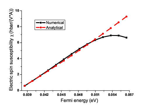
The first term on the right hand side of Eq. (90), resulting from the spin-independent part, is identical to Eq. (67); while the second term, proportional to , can be safely ignored in the low density regime. As shown in Fig. 3, the analytical results of the electric spin susceptibility (Eq. 90) agree well with the numerical ones, demonstrating the applicability of -cubic Rashba model (37) in low doping regime. However, for higher hole density, numerical results show a drop of the due to the heavy and light hole mixing effect, which is certainly beyond the simple -cubic Rashba model.


For numerical results, similar to the derivation above, we may divide into a spin-dependent part and a spin-independent one, namely, . Then the ESS can be expressed as
| (91) |
in which the spin- independent and dependent part respectively reads
| (92) | |||||
| (93) |
Obviously. depends on the average of Fermi wavenumbers, while depends on the Fermi wavenumber difference between two spin-split branches. In most cases, owing to the fact that the spin splitting is small compared with the Fermi energy, will dominate the spin polarization. In Fig. 4(a), we plot the magnitude of spin orientation associated with the subband , denoted by , and the corresponding spin- dependent part, , and independent part . They are related through and . Fig. 4 indicates that for most values of is larger than . Compared to the intra-subband contribution in Fig. 2, the spin-independent magnitude of the spin polarization [green-dotted line in Fig. 4(a)] has similar behavior: first increasing linearly with , then decreasing with increased, and even changing the sign for larger .

A pronounced peak of CISP may appear when the Fermi energy just crosses the bottom of the lowest light hole subband . As amplified in Fig. 5, in the dispersion relation of the subband , the wave numbers corresponding the energy minimum deviate from the point significantly. Around the energy minimum the energy dispersion can be approximated as . Assuming the above energy dispersion and a constant magnitude of , we obtain
| (94) |
where , and and respectively denote two different Fermi wave numbers for (Fig. 5). By Eq. (94) and Fig. 4(b), we can see since and are large in the absolute value but almost opposite in the sign, when , a large spin polarization is expected; on the other hand, when , the contributions of to the spin polarization cancel each other to some extent, resulting in
| (95) |
As is much smaller than or , and , both terms in Eq. (95) are small compared to the case when only is occupied. Apparently, the peak width depends on the spin splitting between and .
The temperature dependence of the peak is plotted in Fig. 6. Near the polarization peak, if we only take into account , ESS is expressed by
| (96) |
At zero temperature, the Fermi distribution function becomes the step-function , which reproduces the above analysis. At finite temperature , if we approximate , and expand the Fermi distribution function at large as ( is Boltzmann constant), then Eq.(96) reduces to
| (97) |
So ESS is proportional to the ratio of the spin splitting of the LH1 subband, , to thermal energy . When is much larger than the spin splitting, this pronounced spin polarization peak will smear out.


Now let’s estimate the magnitude of the averaged CISP. In the -cubic Rashba model with an applied filed , Eq.(50) gives for and for . If typical relaxation time is taken to be and an in-plane electric field strength , the Fermi sphere will be shifted by . Substituting the above data into Eq.(67), we obtain for , and for . Since is proportional to , the spin polarization is very sensitive to the thickness of quantum well. Hence, it is preferable to detect the CISP in a thicker quantum well experimentally. The above estimation gives the same order of magnitude for the spin polarization observed in Silov’s experiment[12]. In Fig. 7, we plot the averaged spin polarization as functions of the Fermi energy and functions of the field in the inset. The CISP is saturated about when the field is enhanced.
V Summary
In conclusion, we have systematically investigate the current induced spin polarization of 2DHG in the frame of the linear response theory. We introduce the physical quantity of the electric spin susceptibility to describe CISP and give its analytical expression in the simplified -cubic Rashba model. Different from the 2DEG, the CISP of 2DHG depends linearly on the Fermi energy. The difference of CISP between 2DHG and 2DEG results from the different spin orientations in the subband of carriers. We propose that -cubic Rashba coefficient of 2DHG can be deduced from the ratio of spin polarization to the current, which is independent of the impurities or disorder effect up to the lowest order. We have also carried out numerical calculations for the CISP. The numerical results are consistent with the analytical one in low doping regime, which demonstrates the applicability of -cubic Rashba model. With the increase of Fermi energy, numerical results show that the spin polarization may be suppressed and even changes its sign. We predict and explain a pronounced spin polarization peak when the Fermi energy crosses over the subband bottom of the . We also discuss the possibility of measuring this spin polarization peak.
Acknowledgements.
This work was supported by the Research Grant Council of Hong Kong under Grant No.: HKU 7041/07P, by the NSF of China (Grant No.10774086, 10574076), and by the Program of Basic Research Development of China (Grant No. 2006CB921500).Appendix A Derivation of the -cubic Rashba Hamiltonian
In this Appendix, we present the detailed derivation of the -cubic Rashba model by means of the perturbation method. [37, 41, 35, 36, 42, 43, 44, 45] First we truncate the Hilbert space of the basis wave functions (26) into the subspace with only the lowest eight states . As described in the Sec. II, by comparing the lowest HH and LH subband dispersion with the exact solution, the accuracy of such truncation procedure has been verified. The truncated subspace can be further cast into two sub-groups, and . contains two lowest heavy hole states , while keeps the other six states, , . In this case, the Hamiltonian in the subspace can be written in the form of block matrices as
| (98) |
where
| (99) |
| (100) |
and
Here are given by
| (108) | |||||
| (109) |
| (110) |
| (111) |
Our aim is to perform a transformation which decouples the groups from , i.e. to make the off-diagonal part and vanish up to the first-order in and . We divide the total Hamiltonian (98) into three parts
| (112) |
The first term is the diagonal matrix elements of , given by
| (113) |
with and .
The second term is given by
| (114) |
where . The third term contains the non-diagonal part and
| (115) |
There are three types of perturbation terms in and : (1)The k-linear term couples the state () with (), where and must be of opposite parities due to the presence of ; (2) The k-quadratic term couples () with (); (3) The asymmetric potential couples the states with the same spin index and different parities.
The perturbation procedure is as follows. First will be eliminated by the canonical transformation as
| (116) |
in which is chosen such that
and the matrix elements read
| (117) |
where denotes the energy of the band at the point (k=0). After the canonical transformation, the new Hamiltonian is given by
| (118) |
The , , and have the block-diagonal form, while is non- block-diagonal and contains new terms first-order in . So we divide into three parts again
| (119) |
in which , and . We perform the second canonical transformation , given by
| (120) |
This makes the non-diagonal block matrix zero, leading to the Hamiltonian
| (121) |
Now the non-block-diagonal terms of vanish up to the desired order in and . Finally, by mapping the Hamiltonian into the lowest heavy hole subbands, we obtain the -cubic Rashba Hamiltonian Eq. (37).
To obtain the corresponding spin operators in the lowest heavy hole basis, we should apply the same canonical transformations and to the spin operators (). In the 8-state subspace , we find that the spin operator has the block-diagonal form , because there are no matrix elements between the states with different confinement quantum number . Therefore is a matrix, given respectively by
Appendix B Hole Rashba term
The hole Rashba term has recently attracted many researchers’ attentions. [36, 32, 47] The hole Rashba term breaks the inversion symmetry, [37, 35] and is expressed as
where , is a parameter as already given by Winkler for several materials, [35] and is the field strength. If we neglect other asymmetrical potentials and only consider the Rashba term, then the total Hamiltonian is . Applying the same perturbation procedure as in the appendix A, we find that both the Hamiltonian and the spin operator have the identical structure to the asymmetrical potential case, as well as the same effective mass , and expression Eq. (52), except for the Rashba coefficient given by
| (142) |
and the spin operator parameter
| (143) |
The hole Rashba coefficient here is proportional to , while for the asymmetrical potential case it depends on . So in most realistic quantum wells, the contribution from the asymmetrical potential plays more important role than the hole Rashba term, at least one or two orders of magnitude larger. The physical reason for this may be understood from the origin of the hole Rashba term. The more general form of the Hamiltonian should be , where the multi-band Hamiltonian includes not only the heavy and light hole bands, but also the conduction band, spin split-off band and remote bands. When we project the Hamiltonian into the subspace of the heavy and light hole bands, the combined effects of the and mediated by other bands lead to the hole Rashba term, which has much smaller influence than that coupled by the asymmetrical potential directly. Therefore, hole Rashba term is neglected in the present article for simplicity.
References
- [1] I. Zutic, J. Fabian, and S. Das Sarma, Rev. Mod. Phys. 76, 323 (2004).
- [2] S. A. Wolf, D. D. Awschalom, R. A. Buhrman, J. M. Daughton, S. von Molna, M. L. Roukes, A. Y. Chtchelkanova, D. M. Treger, Science 294, 1488 (2001).
- [3] D. D. Awschalom and M. E. Flatte, Nature Phys, 3, 153 (2007).
- [4] M. I. Dyakonov and V. I. Perel, Phys. Lett. 35A, 459 (1971).
- [5] V. M. Edelstein, Solid State Commun. 73, 233 (1990).
- [6] A. G. Aronov, Yu. B. Lyanda-Geller, and G. E. Pikus, Sov. Phys. JETP 73, 537 (1991).
- [7] A. V. Chaplik, M. V. Entin, and L. I. Magarill, Physica E (Amsterdam) 13, 744 (2002).
- [8] J. I. Inoue, W. Bauer, and W. Molenkamp, Phys. Rev. B 67, 033104 (2003).
- [9] O. Bleibaum, Phys. Rev. B 73, 035322 (2006).
- [10] O. Bleibaum, Phys. Rev. B 72, 075366 (2005).
- [11] Y. J. Bao and S. Q. Shen, Phys. Rev. B 76, 045313 (2007).
- [12] A. Yu. Silov, P. A. Blajnov, J. H. Wolter, R. Hey, K. H. Ploog, and N. S. Averkiev, Appl. Phys. Lett 85, 5929 (2004).
- [13] Y. Kato, R. C. Myers, A. C. Gossard and D. D. Awschalom, Nature (London) 427, 50 (2004).
- [14] Y. Kato, R. C. Myers, A. C. Gossard, and D. D. Awschalom, Phys. Rev. Lett. 93 176601 (2004).
- [15] V. Sih, R. C. Myers, Y. K. Kato, W. H. Lau, A. C. Gossard and D. D. Awscholom, Nature Physics, 1, 31 (2005).
- [16] N. P. Stern, S. Ghosh, G. Xiang, M. Zhu, N. Samarth, and D. D. Awschalom, Phys. Rev. Lett. 97 126603 (2006).
- [17] C. L. Yang, H. T. He, L .Ding, L. J. Cui, Y. P. Zeng, J. N. Wang, and W. K. Ge, Phys. Rev. Lett. 96, 186605 (2006).
- [18] S. D. Ganichev, S. N. Danilov, P. Schneider, V. V. Belkov, L. E. Golub, W. Wegscheider, D. Weiss, W. Prettl, J. Magn. Magn. Mater. 300, 127 (2006).
- [19] S. D. Ganichev and W. Prettl, J. Phys. Condens. Matter 15, R935 (2003), and references therein.
- [20] X. D. Cui, S. Q. Shen, J. Li, Y Ji, W K. Ge, and F. C. Zhang, Appl. Phys. Lett. 90, 242115 (2007).
- [21] M. G. Vavilov, Phys. Rev. B 72, 195327 (2005).
- [22] S. A. Tarasenko, Phys. Rev. B 72, 153103 (2005).
- [23] M. Trushin and J. Schliemann, Phys. Rev. B 75 , 155323 (2007).
- [24] Z. A. Huang and L. B. Hu, Phy. Rev. B 73, 113312 (2006).
- [25] X. H. Ma, L. B. Hu, R. B. Tao, and S. Q. Shen Phys. Rev. B 70, 195343 (2004).
- [26] L. B. Hu, J. Gao, and S. Q. Shen, Phys. Rev. B 70, 235323 (2004).
- [27] B. Kaestner, D. G. Hasko, and D. A. Williams, cond-mat/0411130.
- [28] B. Kaestner, PhD dissertation, University of Cambridge (2003).
- [29] A. Yu. Silov, J. E. M. Haverkort, N. S. Averkiev, P. M. Koenraad, and J. H. Wolter, Phys. Rev. B 50, 4509 (1994).
- [30] J. M. Luttinger, and W. Kohn, Phys. Rev. 97, 869 (1955); J. M. Luttinger, Phys. Rev. 102, 1030 (1956).
- [31] B. A. Bernevig, T. L. Hughes and S. C. Zhang, Phys. Rev. Lett. 95, 066601 (2005).
- [32] B. A. Bernevig and S. C. Zhang, Phys. Rev. Lett. 95, 016801 (2005).
- [33] J. Schliemann and D. Loss, Phys. Rev. B 71, 085308 (2005).
- [34] J. Sinova, S. Murakami, S. Q. Shen, and M. S. Choi, Solid State Communi.138, 214 (2006)
- [35] R. Winkler, Spin-Orbit Coupling Effects in Two-Dimensional Electron and Hole Systems, (Springer-Verlag Berlin 2003).
- [36] R. Winkler, Phys. Rev. B 62, 4245 (2000).
- [37] B. F. Zhu and Y. C. Chang, Phys. Rev. B 50, 11932 (1994).
- [38] G. D. Mahan, Many-Particle Physics, (Kluwer Academic, New York, 2000).
- [39] P. Streda, J. Phys. C 15, L717 (1982); L. Smrcka and P. Streda, J. Phys. C 10, 2153 (1977).
- [40] N. A. Sinitsyn, J. E. Hill, Hongki Min, Jairo Sinova, and A. H. MacDonald, Phys. Rev. Lett 97, 106804 (2006).
- [41] S. Q. Shen and Z. D. Wang, Phys. Rev. B 61, 9532 (2000)
- [42] B. A. Foreman, Phys. Rev. Lett, 84, 2505 (2000).
- [43] B. A. Foreman, Phys. Rev. B 72, 165344 (2005).
- [44] B. A. Foreman, Phys. Rev. B 72, 165345 (2005).
- [45] B. Habib, E. Tutuc, S. Melinte, M. Shayegan, D. Wasserman, S. A. Lyon, and R. Winkler, Phys. Rev. B 69, 113311 (2004).
- [46] K. Huang, J. B. Xia, B. F. Zhu, and H. Tang, J. Lumin. 40- 41, 88 (1988)
- [47] M. M. Hasegawa and E. A. de Andrada e Silva, Phys. Rev. B 68, 205309 (2003).