The thesis will present results in Quantum Chromo Dynamics (QCD) with dynamical lattice fermions. The topological susceptibilty in QCD is determined, the calculations are carried out with dynamical overlap fermions. The most important properties of the quark-gluon plasma phase of QCD are studied, for which dynamical staggered fermions are used.

Chapter 1 Introduction

The theory of the strong interaction is known to be Quantum Chromo Dynamics (QCD). It has all the features which are necessary for a successful description of the strong interaction. There are very important reasons why it is necessary to invest a lot of effort to solve QCD:

•

Validate or invalidate QCD by comparing its predictions with experiments. Results in the high energy regime show very good agreement with the experiments, however there are still many white areas with no results at all, among them is the missing connection between nuclear physics and QCD.
•

Validate or invalidate the Standard Model of particle physics. Even if QCD is the proper theory of strong interactions, it can happen that the weak and electromagnetic interactions are not correctly described by Standard Model. Examining weak decays can only be done by taking into account low-energy strong interaction effects. The success of the (in)validation is now mostly depends on the precision of QCD calculations.
•

Unfold the phase diagram and properties of QCD at finite temperature and baryon densities. In parallel with the theoretical developments intensive experimental work is done (and will be done) to produce and investigate the high temperature phase of QCD: the quark-gluon plasma. Among these investigations the major goal is to find signals of a first-order or second-order transition.

Solving the above problems is known to be extremely difficult. Currently available methods (e.g.. weak coupling perturbation, $1/N_{c}$ expansion¹¹ 1 $N_{c}$ is the number of colors, in QCD $N_{c}=3$ ., string theory methods, lattice) are not able to provide us with rigorous solutions. However some of these methods are believed to give us very good approximations of these solutions.

Today the lattice technique is the only which is (or will soon be) able to calculate masses of hadrons, properties of low energy scattering processes, bulk and spectral properties of the quark-gluon plasma and many more based only on the Lagrangian of QCD. It contains systematical errors, however these can be quantified, therefore can be kept under control. In the following short introduction to the lattice technique we will highlight the role of ”dynamical fermions” in lattice QCD.

1.1 Dynamical fermions in lattice QCD

Lattice QCD discretizes²² 2 Introductory materials covering the extended literature are [1, 2, 3]. Annual review of the field can be found in the lattice conference proceedings. To avoid the proliferation of citations in the introduction we refer to these, and cite articles only in special cases. the path integral ( $Z$ )

\displaystyle Z=\int[dU][d\psi_{f}][d\bar{\psi}_{f}]\exp(-S_{\rm gauge}-\sum_{f}\bar{\psi_{f}}D[U]\psi_{f})

(1.1)

on a four dimensional Euclidean lattice. The Euclidean space formalism is useful for obtaining the spectrum of the theory or for doing finite temperature calculations. The Minkowski space approach, which is necessary to investigate real time processes, is not available (however see [4]). In Eq. 1.1 we have an integral over the gauge ( $U$ ) and flavored fermion fields ³³ 3 For simplicity we have same quark masses for the different flavors in this introductory section. ( $\bar{\psi_{f}},\psi_{f}$ ). The $S_{\rm gauge}$ is the gauge action, the fermion action is bilinear in the fermion fields, so the fermion integral can be easily carried out. We end up with the determinant of the Dirac-operator ( $D[U]$ ) under the path integral:

\displaystyle Z=\int[dU]\det D[U]^{n_{f}}\exp(-S_{\rm gauge}),

(1.2)

with $n_{f}$ being the number of fermion flavors. The minimal distance on the lattice is called lattice spacing ( $a$ ). The final results are obtained by sending the lattice spacing to zero together with doing some necessary renormalization.

There are two important observations: firstly the Euclidean path integral is equivalent with a Boltzmann sum of a statistical mechanical system and secondly the discretized path integral in a finite volume can be put on a computer. These properties made lattice QCD a multidisciplinary science: it is a mixture of quantum field theory, statistical physics, numerical analysis and computer science. The development in computer algorithms and the exponential rise of the available computational capacity made lattice QCD from a toy model to a powerful predictive tool, giving us high precision pre- and postdictions in a huge number of areas.

Nowadays the calculations are reaching the % level precision thanks to the gradual elimination of the so called quenching effects. Quenching means approximating the fermion determinant with a constant, $U$ independent value in Eq. 1.1 and keeping fermions only in the correlation functions. It is used to decrease the computational requirements, since taking into account the fermion determinant in the path integral (in other words dealing with the fermions dynamically) is a hard task. One can look on the system of 1.1 as a gauge system but with a highly nonlocal⁴⁴ 4 Nonlocality is driven by the smallness of the quark mass. effective action:

S_{\rm eff}=S_{\rm gauge}-n_{f}\log\det D.

Developing efficient algorithms for such systems is nontrivial, however there is a considerable progress in the last years.

There is a huge arbitrariness in choosing the type of the discretization, only a few requirements are to be fulfilled: eg. it should have appropriate symmetries or there should exist an equivalent local formulation. Universality, a well-known concept from statistical physics ensures that in the zero lattice spacing limit the results will not depend on the choice of the discretization. Since the cost of algorithms usually goes with an enormous power of the inverse lattice spacing, in practice it is desirable to improve the lattice actions, that is to reduce their lattice artefacts to make the continuum extrapolations easier from the available lattice spacings. However one should be careful with the improvement: overimproving can lead to several practical problems (loss of locality, unitarity, irregular continuum limit, slowing down of algorithms etc.).

Even there is a possibility that for the fermion determinant and for the fermion correlation functions one uses different discretizations (the first are called sea, the latter are the valence fermions). This is the so called mixed approach. Then the expensive, improved fermion is used in the valence sector, whereas for the sea fermions a faster, less improved is chosen. The correct continuum limit is again ensured by universality.

The design of lattice fermion actions is hindered by the fermion doubling problem. Naive discretization of the continuum Dirac action yields 16 fermions on the lattice. There are three different ways to cure this: staggered, overlap and Wilson fermions. Let us take a brief look on all of them.

Fast, but ugly⁵⁵ 5 For a recent review on the staggered controversy see [5].: staggered fermions

The naive fermion determinant containing 16 fermions has an $U(4)\times U(4)$ symmetry, which can be eliminated by the staggering transformation. This reduces the degeneracy from 16 to four. To get one out of the remaining four fermions one applies the fourth root trick:

\displaystyle\det D[U]\Longrightarrow\det D_{\rm st}[U]\Longrightarrow(\det D_{\rm st}[U])^{1/4}.

(1.3)

The quark correlation functions are usually⁶⁶ 6 Other than staggered quark discretizations are often used in the correlation functions, these are the so called mixed approaches with staggered sea quarks. calculated with the four flavor operator $D_{\rm st}$ .

The main advantage of staggered fermions is that the $D_{\rm st}$ operator has a $U(1)_{\epsilon}$ symmetry in the massless case at any finite lattice spacing. This symmetry corresponds to the flavor non-singlet axial symmetries in the continuum, an important organizing principle in low-energy QCD. Thanks to this symmetry the spectrum of $D_{\rm st}$ is bounded from below, making staggered algorithms well-conditioned. The bare quark mass is only multiplicatively renormalized. These make the simulations fast and convenient.

The major problem is that no local theory is known to correspond to the fourth-root trick, which can be a danger for the universality of the theory. Which means that it can happen that results of staggered lattice QCD differ from that of other discretizations. However any attack against staggered QCD is in a hard position, it should give account for the remarkable agreement between staggered lattice results and real world.

There is an explicit example [6], where fourth root trick gives an incorrect result: case of one massless fermion. According to the anomaly the chiral condensate should acquire some nonvanishing value in the continuum limit with a proper fermion discretization. However due to the $U(1)_{\epsilon}$ symmetry of staggered fermions, the staggered chiral condensate is always exactly zero at any finite lattice spacing (in a finite volume), making staggered fermions fail at this setup.

Usual calculations are done with unphysical, large pion masses, and then an extrapolation to the physical pion mass is carried out (staggered chiral perturbation theory). These extrapolations are controlled by several parameters ( $O(40)$ in NLO for the kaon bag constant), which can make them very ill-conditioned.

Glorious, but slow: chiral fermions

According to the Nielsen-Ninomya theorem eliminating the doubling problem is equivalent with violating continuum chiral symmetry ( $\{D,\gamma_{5}\}=0$ ) on the lattice. The idea of Ginsparg and Wilson was to find a Dirac-operator satisfying

\displaystyle\{D,\gamma_{5}\}=2D\gamma_{5}D.

(1.4)

Only much later was it realized, that this relation makes possible to maintain the chiral symmetry at finite lattice spacing, for which an $O(a)$ redefinition of the chiral transformation is needed. All continuum relations related to chiral symmetry (Ward identities, index theorem, low energy theorems, continuum chiral perturbation theory) are one to one applicable at finite $a$ using a fermion satisfying this relation. The overlap fermion and the fixed-point fermion are the known solutions of Eq. 1.4, whereas the domain-wall fermion provides an approximation to such operators.

The price of these nice properties is quite high: one ends up with a non-ultralocal Dirac-operator (there are interactions between points at any distance), which results in O(100) times or more slower algorithms compared to other discretizations.

The determinant of a Ginsparg-Wilson Dirac-operator will have discontinuities in the space of gauge fields at the topological sector boundaries, just as the continuum Dirac-operator. It is a feature from one hand, on the other hand these jumps makes the conventional dynamical fermion algorithms with chiral Dirac-operators to slow down considerably.

Robust: Wilson fermions

Wilson fermions are curing the doubling problem by violating the chiral symmetry drastically. One gets several inconvenient features at a first sight: additive quark mass renormalization, $O(a)$ lattice artefacts (the previous two discretizations have $O(a^{2})$ ), loss of strict spectral bound on the Dirac-operator. Latter yields ill-conditioned, slow algorithms. The absence of the chiral symmetry makes necessary to evaluate renormalization constants at those places where it is trivial in case of staggered or overlap fermions.

Much theoretical and numerical work was done to improve these properties: using smeared gauge links in the fermion action the additive renormalization can be decreased by two orders of magnitude, the $O(a)$ lattice artefacts can be reduced to $O(a^{2})$ via the Symanzik-improvement program, the spectral bound is reported to be recovered in the infinite volume limit [7].

These made possible to be competitive with the staggered discretization in speed and since it is in much better theoretical shape it might be the choice for the near future.

1.2 Overview of the thesis

The use of dynamical fermions is nowadays obligatory in lattice QCD. Developing new algorithms for dynamical fermions is still an active area of research. In this thesis I will present two dynamical fermion projects in which I have participated.

The first topic, discussed in Chapter 2, deals with the dynamical overlap fermion project in detail. This chapter is partially based on the articles:

•

[8] Z. Fodor, S.D. Katz, K.K. Szabo JHEP 0408:003,2004
•

[9] G.I. Egri, Z. Fodor, S.D. Katz, K.K. Szabo JHEP 0601:049,2006

First I will present our dynamical overlap algorithm, then I will show how the naive algorithm fails to change topological sectors. A new algorithm is proposed and tested, which solves the problem. Finally the topological sector changing of the new algorithm is examined, and attempts to improve it are proposed. I am trying to give a comprehensive review of the field, which also means that only a part of the results belong to me. My contributions are the following:

•

Writing and developing a 5000 line C program for generating overlap fermion configurations.
•

Modifying the conventional HMC algorithm to circumvent its failure at topological sector boundaries.
•

Improving the stepsize dependence of this algorithm.
•

Examining the tunneling behavior of this algorithm.
•

Performing simulations and measuring the topological susceptibility in two flavor QCD.

The second topic is the dynamical staggered project (Chapter 3). This is a large scale computation of thermodynamical properties of the quark gluon plasma. I will describe our choice of action and the algorithmic improvements first. Then I will show our determination on the order of the finite temperature QCD transition in continuum limit and with physical quark masses. Next the transition temperature in physical units is calculated, again in the continuum limit and with physical quark masses. These results can be considered as final ones modulo the uncertainty in the staggered discretization. Finally I will present the equation of state, but there the calculations were only done with two lattice spacings, the continuum limit is missing. The chapter is partially contained in these articles:

•

[10] Y. Aoki, G. Endrodi, Z. Fodor, S.D. Katz, K.K. Szabo Nature 443:675-678,2006
•

[11] Y. Aoki, Z. Fodor, S.D. Katz, K.K. Szabo Phys. Lett. B643:46-54,2006
•

[12] Y. Aoki, Z. Fodor, S.D. Katz, K.K. Szabo JHEP 0601:089,2006

Again not all results belong to me, my contributions are:

•

Writing and developing a 5000 line C program for generating staggered fermion configurations.
•

Performing large scale zero and finite temperature simulations.
•

Analyzing and renormalizing the data.

Chapter 2 Dynamical overlap fermions

Chiral symmetry is one of the most important feature of the strong interaction. Lattice regularization and chiral symmetry were contradictious concepts for many years. Fermionic operators satisfying the Ginsparg-Wilson relation [13]

\displaystyle\{D,\gamma_{5}\}=\frac{1}{m_{0}}D\gamma_{5}D.

(2.1)

made possible to solve the chirality problem of four-dimensional QCD at finite lattice spacing [14, 15, 16, 17].

Several numerical studies with exact chirality operators were done in the quenched approximation [18, 19, 20]. The results were really compelling, but people were forced to work with nonlocal Dirac-operators. This made the algorithms more complicated and slowed them down by large factors. At the same time one could reach rather small quark masses, which was unimaginable with Wilson-type discretizations before.

The life becomes even more complicated when introducing dynamical fermions with exact chirality. This chapter is devoted to this problem. We will going to work with overlap fermions [21, 22], it is an explicit solution of the Ginsparg-Wilson relation. The other type of solutions, the fixed-point Dirac operators [23] are defined via a recursive equation, they are considerably harder to implement¹¹ 1 For dynamical simulation of an approximate fixed-point Dirac operator see [24]..

2.1 Overlap Dirac operator

First we fix our notations. The massless Neuberger-Dirac operator (or overlap operator) $D$ can be written as

D=m_{0}[1+\gamma_{5}{\rm sgn}(H_{W})],

(2.2)

This $D$ operator satisfies Eq. (2.1). $H_{W}$ is the hermitian Dirac operator, $H_{W}=\gamma_{5}D_{W}$ , which is built from the massive Wilson-Dirac operator, $D_{W}$ , defined by

\displaystyle[D_{W}]_{xy}=(4-m_{0})\delta_{xy}-\frac{1}{2}\sum_{\mu}\left\{U_{\mu}(x)(1+\gamma_{\mu})\delta_{x,y-\mu}+U_{\mu}^{\dagger}(y)(1-\gamma_{\mu})\delta_{y,x+\mu}\right\}.

One fermion is obtained in the continuum limit, if $m_{0}$ takes any value between $0$ and $2$ . In a finite volume one should be careful, that the physical branch of the spectrum of the $D_{W}$ operator is to be projected to the physical part of the overlap circle.

The mass is introduced in the overlap operator by

D(m)=(1-\frac{m}{2m_{0}})D+m.

Sometimes it is useful to consider the hermitian version of the overlap operator. Let us review its properties. The massless hermitian overlap operator is $H=\gamma_{5}D=m_{0}(\gamma_{5}+{\rm sgn}(H_{W}))$ . The eigenvalues are real, the eigenvectors ( $|\lambda\rangle$ ) are orthogonal and span the whole space. Due to the Ginsparg-Wilson relation

\displaystyle\{H,\gamma_{5}\}=\frac{1}{m_{0}}H^{2},

(2.3)

the matrix elements of $\gamma_{5}$ satisfy:

\displaystyle\langle\lambda|\gamma_{5}|\mu\rangle(\lambda+\mu)=\frac{\lambda^{2}}{m_{0}}\delta_{\lambda\mu}.

(2.4)

From this equation it follows, that the zeromodes can be chosen to be chiral, furthermore eigenvectors with eigenvalues $\pm 2m_{0}$ have positive/negative chirality. The difference in the number of left and right handed zeromodes is proportional to the trace of $H$ :

\displaystyle\frac{1}{2m_{0}}{\rm Tr}H=\sum_{\lambda}\frac{\lambda}{2m_{0}}=\sum_{\lambda}\langle\lambda|\gamma_{5}|\lambda\rangle-(n(+0)-n(-0))=n(-0)-n(+0).

(2.5)

This difference is called the index of $H$ , it can be considered as the definition of the topological charge on the lattice. This is supported by the fact, that in the continuum limit the density ${\rm tr}H$ converges to $\sim F\tilde{F}$ . Since the right hand side can take only integer values, we can immediately conclude that the overlap operator cannot be continuous function of the gauge fields. It should be nonanalytic on the boundaries of topological sectors.

Further eigenvalues are always coming in pairs, the vector

\displaystyle|-\lambda\rangle=\left(1-\frac{\lambda^{2}}{(2m_{0})^{2}}\right)^{-1/2}\left(\gamma_{5}-\frac{\lambda}{2m_{0}}\right)|\lambda\rangle

(2.6)

is an eigenvector with eigenvalue $-\lambda$ . The $\gamma_{5}$ matrix leaves the subspace $\{|\lambda\rangle,|-\lambda\rangle\}$ invariant, it can be written as

\displaystyle\gamma_{5}=\begin{pmatrix}\frac{\lambda}{2m_{0}}&\left(1-\frac{\lambda^{2}}{(2m_{0})^{2}}\right)^{1/2}\\ \left(1-\frac{\lambda^{2}}{(2m_{0})^{2}}\right)^{1/2}&-\frac{\lambda}{2m_{0}}\end{pmatrix}.

(2.7)

Since $\gamma_{5}$ is traceless on the subspace $\{|\lambda\rangle,|-\lambda\rangle\}$ with $\lambda\neq\{0,\pm 2m_{0}\}$ , it should be also traceless for the $\lambda=\{0,\pm 2m_{0}\}$ space. This requires that the numbers of $\pm 2m_{0}$ eigenmodes satisfy

\displaystyle n(+2m_{0})-n(-2m_{0})=n(-0)-n(+0).

(2.8)

The overlap operator squared $H^{2}(m)$ commutes with $\gamma_{5}$ . This is a trivial fact in the $\lambda=\{0,2m_{0}\}$ subspaces, where even $[H(m),\gamma_{5}]=0$ is true. In $\{|\lambda\rangle,|-\lambda\rangle\}$ subspace it is proportional to the identity matrix

\displaystyle H^{2}(m)=\begin{pmatrix}\left(1-\frac{m^{2}}{(2m_{0})^{2}}\right)\lambda^{2}+m^{2}&0\\ 0&\left(1-\frac{m^{2}}{(2m_{0})^{2}}\right)\lambda^{2}+m^{2}\end{pmatrix}.

(2.9)

2.1.1 Numerical implementation

In the sign function of Eq. (2.2) one uses ${\rm sgn}(H_{W})=H_{W}/\sqrt{H_{W}^{2}}$ . We usually need the action of the ${\rm sgn}(H_{W})$ operator on a given vector, which was studied many times in the literature [25, 26]. The common in all algorithms is that their speed is proportional to the inverse condition number of the matrix $H_{W}$ . To make the algorithms better conditioned, one can project out the few low-lying eigenmodes of the matrix $H_{W}$ and calculate the ${\rm sgn}$ operator in this space exactly:

\displaystyle{\rm sgn}(H_{W})=\sum{\rm sgn}(s)P_{s}+{\rm sgn}(QH_{W}),

(2.10)

where $P_{s}$ is the projector to the $s$ eigenspace of $H_{W}$ and $Q=1-\sum_{s}P_{s}$ . The projections were done by the ARPACK code. To speed up the projections we preconditioned the problem with a Chebyshev-polynomial transformation [27]. We have taken the $n$ -th order approximation of the $\tanh(80(x+1))-1$ function in $[-1,1]$ interval:

\displaystyle T_{n}(x)\approx\tanh(80(x+1))-1.

(2.11)

This blows up very fast around $-1$ . If we concentrate the interesting part of the spectrum of $H_{W}$ there, then we make the job of the eigenvector projecting algorithm considerably easier (its speed usually depends on the distance between consecutive eigenmodes). That is we were calculating the eigenvectors of $T_{n}(H_{W}^{2}/s_{\rm max}^{2}-1)$ instead of those of $H_{W}$ . Since this is only a polynomial transformation, only the eigenvalues are different, the eigenvectors should be the same. The result is that the problem is much better conditioned using Chebyshev-polynomials. The speed gain was almost an order of magnitude.

For the rest of the sign function ( ${\rm sgn}(QH_{W})$ ) one can take her/his favorite approximation: $\sigma(QH_{W})$ . We have considered two of them: Zolotarev rational function and Chebyshev polynomial.

The $n^{\rm th}$ order Zolotarev optimal rational approximation for $1/\sqrt{x}$ in some interval $[x_{\rm min},x_{\rm max}]$ can be expressed by elliptic functions (see e.g. [28]), the coefficients can be also determined by a Remes-algorithm. A particularly useful form of the approximation for the sign function is given by the sum of partial fractions

\sigma_{\rm Zol}(x)=x\left(a_{0}+\sum_{i=1}^{n}{a_{i}\over x^{2}+b_{i}}\right),

(2.12)

in usual cases $n\sim O(10)$ . To get the approximation of the sgn of a matrix $A$ one has to plug the $A$ into Eq. 2.12: ${\rm sgn}(A)\approx\sigma_{\rm Zol}(A)$ . The inversions appearing in this approximation all contain the same matrix but with different shifts ( $b_{i}$ ). There are so-called multishift Krylov-space methods [29, 30], which can solve the system of $n$ inversions with the same number of matrix multiplications as needed to solve only one system. Since matrix multiplications dominate such algorithms, this means that practically for the cost of one inversion one obtains the solutions of $n$ systems. When inverting the multishift system it might be desirable to project out even more eigenvectors than before in Eq. 2.10 and calculate the inverse in this subspace exactly: $(s^{2}+b_{i})^{-1}P_{s}$ .

The Chebyshev-polynomial approximation ( $\sigma_{\rm Cseb}$ ) in principle performs similarly as the Zolotarev rational function. Here one has to make multiplication with the Wilson matrix many times ( $\sim O(100)$ ), there is no need for global summations as in Zolotarev case. There are architectures (eg. Graphical Processing Units [31]), where global summation is a bottleneck, it should be avoided everywhere if possible. In these cases the Chebyshev-approximation is a good choice.

2.2 Hybrid Monte-Carlo

Hybrid Monte-Carlo (HMC, [32]) is the most popular method for simulating dynamical fermions. There are many other choices possible, but HMC outperforms from all of these. We will base our work on the HMC algorithm. One would like to generate gauge configurations via a Monte-Carlo update with the following weight (see 1.1):

\displaystyle w[U]=\exp(-S_{\rm gauge})\det(D^{\dagger}D),

(2.13)

where we have $D^{\dagger}D$ instead of $D^{2}$ for the weight of two fermion flavors. This substitution is legal, since the one flavor fermion determinant is real. The standard procedure to implement the fermion determinant is to rewrite it using bosonic fields, so-called pseudofermions ( $\phi(x)$ ):

\displaystyle w[U]=\exp(-S_{\rm gauge})\int[d\phi^{\dagger}d\phi]\exp(-\phi^{\dagger}(D^{\dagger}D)^{-1}\phi)

(2.14)

Now let us consider the following steps:

1.

Choose Gaussian distributed momenta $P_{\mu}(x)$ .
2.

Choose a $\phi$ field according to the distribution $\exp(-\phi^{\dagger}(D^{\dagger}D)^{-1}\phi)$ .
3.

At a fixed $\phi$ background evolve the $U_{\mu}(x)$ gauge fields and $P_{\mu}(x)$ momenta using the equations of motion derived from the Hamiltonian

$\displaystyle H=\frac{1}{2}P^{2}+S_{\rm gauge}+\phi^{\dagger}(D^{\dagger}D)^{-1}\phi,$ (2.15)

and from the structure of the manifold. The evolution from $(U,P)$ fields to some $(U^{\prime},P^{\prime})$ via the equations of motion is usually called a trajectory.

Iterating steps from 1. to 3. one obtains a chain of gauge configurations with the distribution Eq. 2.13. Along a trajectory the energy and the area are conserved, moreover these trajectories are exactly reversible. To determine the trajectories is an infinitely hard problem, it requires an exact solution of the equations of motion.

However an approximate solution of these equations can be also used to build a chain of gauge configurations with the exact $w[U]$ distribution. One just has to find an area preserving and reversible integrator and integrate the equations approximately with it. With such an integrator at hand one trajectory will be generated via the following procedure:

1.

As before.
2.

As before.
3.

Integrate the equations of motion with an approximate integrator.
4.

Calculate the energy difference: $\Delta H=H(U^{\prime},P^{\prime})-H(U,P)$ and accept/reject the configuration with the probability ${\rm min}(1,\exp(-\Delta H))$ .

This is one iteration of the HMC algorithm. This iteration also produces configurations with the same equilibrium distribution (Eq. 2.13) as the previous one.

The easiest area conserving and reversible integrator is the leapfrog. The leapfrog integration consist of making $1/\epsilon$ of the following steps²² 2 In case of unit length trajectories.:

\displaystyle\mathcal{U}(\epsilon/2)\mathcal{P}(\epsilon)\mathcal{U}(\epsilon/2),

(2.16)

where $\mathcal{U}$ operator evolves the gauge fields with the actual (fixed) momenta, wheres $\mathcal{P}$ operator evolves the momenta using the force calculated at the actual (fixed) gauge field. The $\epsilon$ is called the stepsize, obviously in the $\epsilon\to 0$ limit one arrives to the exact solution of the equations of motion. The energy is violated by $O(\epsilon^{3})$ by making one leapfrog step, during $1/\epsilon$ steps of a unit length trajectory this error grows up to $O(\epsilon^{2})$ . The average energy conservation violation can be shown to be $\langle\Delta H\rangle=C\epsilon^{4}+\dots$ . Since $C$ is most generally proportional to the volume, the stepsize should be decreased as $\epsilon\sim V^{-1/4}$ to keep constant acceptance.

Using area conservation and reversibility one can show that the condition

\displaystyle\langle\exp(-\Delta H)\rangle=1

(2.17)

should be satisfied, this relation provides an easy check of the consistency of the algorithm. This condition also shows us that if one has large energy conservation violations ( $|\Delta H|\gtrsim 1$ ), then the acceptance should be small. In this case one should decrease the stepsize to obtain a good acceptance. The optimal acceptance rate depends on the type of the integrator, in case of the leapfrog and its variants the optimum is around $80\%$ .

Even one can drop away the area preservation property for the evolution of the gauge fields and momentum, in this case one has to include the Jacobian of the mapping into the accept/reject step.

2.2.1 HMC for two flavors of overlap fermions

In case of the overlap fermion the gauge field and momentum evolution is the following:

\displaystyle\mathcal{U}(\epsilon):U\to\exp(\epsilon P)U,

\displaystyle\mathcal{P}(\epsilon):P\to P-\epsilon\mathcal{A}\left[U\frac{\partial}{\partial U}\left(S_{\rm gauge}+S_{\rm pf}\right)\right],

(2.18)

where in the force term the $\mathcal{A}$ operator projects onto traceless, antihermitian matrices (in color indices). The complication arises in the derivative of $S_{\rm pf}$ , which schematically can be written as

\displaystyle\delta S_{\rm pf}=-\psi^{\dagger}\delta(D^{\dagger}D)\psi\qquad\qquad{\rm with}\qquad\qquad\psi=(D^{\dagger}D)^{-1}\phi.

(2.19)

The inversion of the fermion operator $\psi=(D^{\dagger}D)^{-1}\phi$ is done by $n_{o}$ conjugate gradient³³ 3 For studies with inverters other than conjugate gradient see [33]. steps (”outer inversion”). Note, however, that each step in this procedure needs the calculation of $(D^{\dagger}D)\phi$ . The operator $D$ contains $\sigma(H_{W})$ , which is given for example by the partial fraction expansion (see Eq. 2.12). Thus, at each ”outer” conjugate gradient step one needs the inversion of the $H_{W}^{2}$ matrix (”inner inversion”). This nested type of the inversions is the price one has to pay for an exactly chiral Dirac-operator, in other formulations one only has one matrix inversion per force calculation. No method is known to avoid the nested inversions.

The $\delta(D^{\dagger}D(m))=\delta(H(m)^{2})$ derivative has a complicated form. Let us assume, that we treat the sgn function in the overlap operator as in Eq. 2.10. Then the derivative of $H(m)$ will have two parts

\displaystyle\delta H(m)=\delta_{1}H(m)+\delta_{2}H(m).

(2.20)

The first part will contain the derivative of the projectors ( $P_{s}=|s\rangle\langle s|$ ), this term comes not only as a derivative of $\sum{\rm sgn}(s)P_{s}$ , but the projectors are also there in the $Q{\rm sgn}(H_{W})$ term. All together one obtains

\displaystyle\delta_{1}H(m)=\left(m_{0}-m/2\right)\sum_{s}\delta P_{s}({\rm sgn}(s)-\sigma(H_{W})).

(2.21)

The derivative of the projector can be derived with the tools of quantum mechanical perturbation theory [34]:

\displaystyle\delta P_{s}=-\left(\frac{1-P_{s}}{H_{W}-s}\delta H_{W}P_{s}+P_{s}\delta H_{W}\frac{1-P_{s}}{H_{W}-s}\right).

(2.22)

As we can see each projected mode brings an extra inversion of the (shifted) Wilson matrix. It might be safe to treat the few lowest lying modes of $H_{W}$ this way, but it is meaningless to calculate exactly the force of modes from the bulk of the spectrum.

The second term in $\delta H(m)$ will be the derivative of the sgn function approximation ( $\delta_{2}H(m)$ ). In case of the Zolotarev approximation one has

\displaystyle\delta\sigma_{\rm Zol}(A)=\delta A\left(a_{0}+\sum_{i=1}^{n}\frac{a_{i}}{A^{2}+b_{i}}\right)-\sum_{i=1}^{n}\frac{a_{i}}{A^{2}+b_{i}}(A^{2}\delta A+A\delta AA)\frac{a_{i}}{A^{2}+b_{i}},

(2.23)

therefore the contribution to the derivative of $H(m)$ is

\displaystyle\delta_{2}H(m)=(m_{0}-m/2)Q\delta\sigma_{\rm Zol}(H_{W}).

(2.24)

In case of the polynomial approximation the formula is more complicated.

The sgn function is needed as three different places during the HMC trajectory: in the force calculation one needs $H(m)^{-2}$ and $\delta H(m)$ and in the action calculation one needs $H(m)^{-2}$ again. The presence of the accept/reject step allows one to use different approximations at different places. One can speed up the algorithm with large factors by carefully choosing and tuning the approximations. We were using the Chebyshev polynomial approximation in the inversions with O(20) projected modes whereas for the $\delta H(m)$ we chose the Zolotarev rational approximation with 2 projected modes. The relative precision was always set to $10^{-6}$ everywhere.

For somewhat different implementations of the standard HMC and for various improvement techniques we refer here to the work of two other groups [35, 36, 37, 38].

2.2.2 Criticism of the HMC for one fermion flavor

The HMC described above works only for a positive definite fermion matrix. This is suitable for two flavors. For one flavor one can take the square root of the squared operator (RHMC algorithm). A different way to get the square root of the fermion determinant is to exploit the exact chiral symmetry of the Dirac-operator [39, 40]. As we have seen before $H(m)^{2}$ has $n(+0)+n(-0)$ chiral modes with eigenvalue $m^{2}$ , $n(2m_{0})+n(-2m_{0})$ chiral modes with eigenvalue $(2m_{0})^{2}$ and all the other modes are doublets with eigenvalue $\left(1-\frac{m^{2}}{(2m_{0})^{2}}\right)\lambda^{2}+m^{2}$ . It is a conventional wisdom that only those configurations contribute to the path integral where either $n(+0)=0$ or $n(-0)=0$ . If this is true then we can write the two flavor fermion determinant as

\displaystyle n(\pm 0)=0:\quad\quad\det H(m)^{2}={\rm det}_{\pm}H(m)^{2}{\rm det}_{\mp}H(m)^{2}=[{\rm det}_{\pm}H(m)^{2}]^{2}\left(\frac{m^{2}}{(2m_{0})^{2}}\right)^{n(\mp 0)},

where the ${\rm det}_{\pm}$ determinants have to be restricted to positive/negative chirality subspaces. The numerical factor at the end of the formula takes into account that the zeromodes and $\pm 2m_{0}$ modes are not coming in chirality pairs (see Eq. 2.8). At this point it is easy to perform the square root

\displaystyle\det H(m)=\left(\frac{m}{(2m_{0})}\right)^{n(\mp 0)}{\rm det}_{\pm}H(m)^{2},

(2.25)

where the sign depends on the chirality of the zero modes of $H$ . Since $H(m)^{2}$ is positive definite even on the definite chirality subspaces, there is no obstacle to introduce pseudofermions for its determinant. The contribution of the zeromodes and $\pm 2m_{0}$ modes can be taken into account by reweighting the observables with them.

One has to face with the following problem. Let us consider a trajectory which starts with a gauge configuration where $n(+0)=0$ and ends where $n(-0)=0$ . The pseudofermion is generated at the beginning of the trajectory according to the distribution:

\displaystyle\exp(-\phi^{\dagger}H(m)^{-2}P_{+}\phi),

(2.26)

where $P_{+}$ projects on positive chirality. If one consider the reversed trajectory (starting from the sector, where $n(-0)=0$ ) the pseudofermion distribution is

\displaystyle\exp(-\phi^{\dagger}H(m)^{-2}P_{-}\phi),

(2.27)

with $P_{-}$ negative chirality projector. This means that the reversed trajectory uses a different pseudofermion distribution than the original one. For the proof of the detailed balance one needs to have the same pseudofermion distribution on both ends. This algorithm yields the violation of the detailed balance for trajectories where the ends are in topological sectors with different signs. The usual way out is that the trajectories are constrained to that part of the phase space where e.g. $n(+0)=0$ is always satisfied. However this choice opens the way of a possible ergodicity breaking, which is also hard to keep under control.

2.3 Reflection/refraction

In the previous section we have shown how to set up the traditional HMC for overlap fermions. Performing simulations on rather small ( $6^{4}$ ) lattices the acceptance rate was almost zero. The strange thing was that decreasing the stepsize of the integrator did not help at all. Tracing down the problem, one finds that there are sudden jumps in the microcanonical energy during the trajectories. These jumps are usually in the order of O(10) or larger, the trajectories where the energy violations are of this size are practically never accepted in the final accept/reject step.

These jumps occur at the discontinuity of the overlap operator, that is at the topological sector boundaries. The phenomena can be nicely observed in the spectrum of the hermitian Wilson-Dirac operator. The topological charge can be written as

\displaystyle Q=\frac{1}{2m_{0}}{\rm Tr}H=\frac{1}{2}\sum_{s}\langle s|\gamma_{5}+{\rm sgn}(H_{W})|s\rangle=\frac{1}{2}\sum_{s}{\rm sgn}(s),

(2.28)

where $s$ ’s are the real eigenvalues of $H_{W}$ . The charge changes when an eigenvalue of $H_{W}$ crosses zero. At this point most presumably the overlap operator itself is discontinuous, since its trace is discontinuous. This means that the pseudofermion action also has a discontinuity, which means a Dirac-delta in the fermion force. Obviously a finite-stepsize integrator will never notice the presence of a Dirac-delta in the force. Without any correction one will end up with an energy violation which is roughly the discontinuity in the fermion action.

One can improve on this situation. This feature is already present in a classical one-dimensional motion of a point-particle in a step function potential. During the integration one should check whether the particle moved from one side to the other one of the step function. If it is necessary, one corrects its momentum and position. This correction has to be done also in the case of the overlap fermion. The microcanonical energy,

H=\frac{1}{2}P^{2}+S_{\rm gauge}[U]+S_{\rm pf}[U,\phi]=\frac{1}{2}P^{2}+S[U,\phi]

(2.29)

has a step function type non-analyticity on the the zero eigenvalue surfaces of the $H_{W}$ operator in the space of link variables coming from the pseudofermion action. When the microcanonical trajectory reaches one of these surfaces, we expect either reflection or refraction. If the momentum component, orthogonal to the zero eigenvalue surface, is large enough to compensate the change of the action between the two sides of the singularity ( $\Delta S$ ) then refraction should happen, otherwise the trajectory should reflect off the singularity surface. Other components of the momenta are unaffected. The anti-hermitian normal vector ( $N$ ) of the zero eigenvalue surface can be expressed with the help of the gauge derivative as

\displaystyle N\sim\langle s|\mathcal{A}\left(U\frac{\partial H_{W}}{\partial U^{T}}\right)|s\rangle,

(2.30)

where $\mathcal{A}$ projects to the antihermitian, traceless matrices in color space. Table 2.1 summarizes the conditions of refraction and reflection and the new momenta.

	When	New momenta
Refraction	$(N,P)^{2}>2\Delta S$	$P-N(N,P)+N(N,P)\sqrt{1-2\Delta S/(N,P)^{2}}$
Reflection	$(N,P)^{2}<2\Delta S$	$P-2N(N,P)$

Table 2.1: Refraction and reflection can happen to the system when approaches a zero eigenvalue surface of

H_{W}

. The conditions and the new momenta are indicated.

P

is the momentum before the refraction/reflection.

2.3.1 Modified leapfrog

We have to modify the standard leap-frog integration of the equations of motion in order to take into account reflection and refraction. This can be done in the following way. The standard leap-frog consists of three steps: an update of the links with stepsize $\epsilon/2$ , an update of the momenta with $\epsilon$ and finally another update of the links, using the new momenta, again with $\epsilon/2$ , where $\epsilon$ is the stepsize of the integration. The system can only reach the zero eigenvalue surface during the update of the links. We have to identify the step in which this happens. After identifying the step in which the zero eigenvalue surface is reached, we have to replace it with the following three steps:

1.

Update the links with $\epsilon_{c}$ , so that we reach exactly the zero eigenvalue surface. $\epsilon_{c}$ can be determined with the help of $N$ .
2.

Modify the momenta according to Table 2.1.
3.

Update the links using the new momenta, with stepsize $\epsilon/2-\epsilon_{c}$ .

This means that in leapfrog step of Eq. 2.16 we have to substitute the appropriate $\mathcal{U}(\epsilon/2)$ operator with

\displaystyle\mathcal{U}_{\rm mod}(\epsilon/2)=\mathcal{U}(\epsilon_{c})\mathcal{R}\mathcal{U}(\epsilon/2-\epsilon_{c}),

(2.31)

where $\mathcal{R}$ is the refraction/reflection operator, which changes the momenta according to Tab. 2.1. This procedure is trivially reversible and it also preserves the integration measure as shown in the appendix of this chapter.

where $P^{\prime}=\mathcal{R}P$ is the reflected/refracted momentum. $F=\mathcal{A}\left(U\frac{\partial S}{\partial U^{T}}\right)$ is the force evaluated at the topological sector boundary on the starting side, which means that the undefined ${\rm sgn}(0)$ in $F$ is interpreted as ${\rm sgn}(s-)$ . $F^{\prime}$ is also evaluated on the boundary, but with ${\rm sgn}(0)={\rm sgn}(s+)$ . Obviously $F^{\prime}=F$ in case of a reflection. The energy violation of Eq. 2.32 can be a serious problem, since a $(P,F)$ type quantity is in general proportional to the volume. Which means that one has to decrease the stepsize with $\epsilon\sim V^{-1}$ to keep the acceptance constant. This is much worse than the original $\epsilon\sim V^{-1/4}$ scaling of the leapfrog.

Fig. 2.1 compares the evolution of the energy and lowest $\lambda$ for the usual and for the modified leapfrog. In the unmodified case there is a huge energy jump at the crossing, the trajectory is most probably rejected. Whereas in the modified case a reflection happens, and $\mathcal{H}$ is much better conserved.

Refer to caption — Figure 2.1: Comparison of the unmodified (triangles) and modified (boxes) leapfrogs. Upper part is the energy, lower part is the lowest mode of $H_{W}$ .

There is one bottleneck however. If we correct only for the discontinuity in the potential as above, then the microcanonical energy violation will be proportional to the stepsize. That is for a $\mathcal{U}_{\rm mod}(\epsilon/2)\mathcal{P}(\epsilon/2)$ step the energy violation is

\displaystyle\Delta H=\epsilon_{c}((P^{\prime},F^{\prime})-(P,F))+O(\epsilon^{2}),

(2.32)

2.3.2 Improving the modified leapfrog

There are several ways out of the problem. We will consider two variants in this section:

•

Reflection/refraction step with $C\epsilon$ energy violation, the $C$ coefficient being only an $O(1)$ size number instead of $O(V)$ , which means that the bad scaling is eliminated.
•

Reflection procedure with $O(\epsilon^{2})$ energy violation.

In the literature there exists a reflection/refraction procedure with $O(\epsilon^{2})$ energy violation [37], however it is somewhat more complicated than these two improvements.

The large energy conservation violation of $\mathcal{U}_{\rm mod}$ arises, since not the appropriate momentum is reflected/refracted. If one inserts two extra momentum updates into Eq. 2.31

\displaystyle\mathcal{U}(\epsilon_{c})\mathcal{P}(\epsilon_{c})\cdot\mathcal{R}\cdot\mathcal{P}(\epsilon/2-\epsilon_{c})\mathcal{U}(\epsilon/2-\epsilon_{c}),

(2.33)

then the energy is conserved upto $O(\epsilon^{2})$ . This is due to the fact that both $\mathcal{U}(\epsilon)\mathcal{P}(\epsilon)$ and $\mathcal{P}(\epsilon)\mathcal{U}(\epsilon)$ conserves the energy upto $O(\epsilon^{2})$ and $\mathcal{R}$ conserves the energy exactly. This step however violates the area conservation upto $O(\epsilon)$ , there is no free lunch.

The first idea is based on the fact, that if one makes the extra momentum updates only in the space, which is orthogonal to the normalvector $N$

\displaystyle\mathcal{U}(\epsilon_{c})\mathcal{P}_{\bot}(\epsilon_{c})\cdot\mathcal{R}\cdot\mathcal{P}_{\bot}(\epsilon/2-\epsilon_{c})\mathcal{U}(\epsilon/2-\epsilon_{c}),

(2.34)

then the area is exactly conserved again (as shown in the appendix). Now the energy is still violated by $O(\epsilon)$ terms, but since the update in the orthogonal space is done $O(\epsilon^{2})$ correctly, their coefficients is only an $O(1)$ number. The stepsize should be decreased only as $\epsilon\sim V^{-1/2}$ .

The second idea applies only for the reflection. It uses the following observation. In a one dimensional case if the time required to reach the boundary ( $\epsilon_{c}$ ) and the time which is required to step away from the boundary ( $\epsilon/2-\epsilon_{c}$ ) are the same, then as a result of the reflection step, the trajectory has been exactly reversed. The area conservation, reversibility are obviously preserved, the energy is conserved exactly. We can try whether these remain true in arbitrary dimensions (the area conservation is proven in the appendix, the exact reversibility and energy conservation upto $O(\epsilon^{2})$ are obvious). Then we should insert a

\mathcal{U}(\epsilon_{c})\mathcal{P}(\epsilon_{c})\mathcal{R}\mathcal{P}(\epsilon_{c})\mathcal{U}(\epsilon_{c})

(2.35)

step into the chain of leapfrogs, when the boundary is hit. In Eq. 2.16 we have written the elementary leapfrog step in the $UPU$ form, now let us write it in the $PUP$ order:

\mathcal{P}(\epsilon/2)\mathcal{U}(\epsilon)\mathcal{P}(\epsilon/2),

(2.36)

Now we split the evolution of the links into two parts:

\mathcal{P}(\epsilon/2)\mathcal{U}(\epsilon/2)\cdot\mathcal{U}(\epsilon/2)\mathcal{P}(\epsilon/2).

(2.37)

Consider that the boundary would be crossed during one of the evolutions of the links in Eq. 2.37. Then replace the original leapfrog with the following:

\mathcal{P}(\epsilon/2)\mathcal{U}(\epsilon/2)\cdot\mathcal{U}(\epsilon_{c})\mathcal{P}(\epsilon_{c})\mathcal{R}\mathcal{P}(\epsilon_{c})\mathcal{U}(\epsilon_{c})\cdot\mathcal{U}(\epsilon/2)\mathcal{P}(\epsilon/2).

Now $\epsilon_{c}$ is the time to reach the boundary surface measured from the midpoint of the leapfrog. Thus if the crossing would happen in the first evolution then $\epsilon_{c}<0$ , if in the second, then $\epsilon_{c}>0$ .

2.3.3 Tracing the evolution of low lying eigenmodes

We have to trace the evolution of the low lying eigenmodes, since we are looking for the moment when one eigenvalue crosses zero. The eigenvectors and eigenvalues are available at discrete times only (once or twice per time step), therefore one has to pair the eigenvectors at time $t$ and time $t+\epsilon$ . We calculated the scalar products $\langle s^{\prime}(t+\epsilon)|s(t)\rangle$ after each link update, and our recipe was the following: the $s(t)$ has evolved to that $s^{\prime}(t+\epsilon)$ with which the scalar product was maximal. Of course this can break down if the time step is too large. It is easy to show, that to make this naive method work one has to decrease the stepsize as the volume is increased with $\sim V^{-1}$ . Expanding the $\langle s^{\prime}(t+\epsilon)|s(t)\rangle$ one obtains:

\displaystyle\langle s^{\prime}(t+\epsilon)|s(t)\rangle=\delta_{s^{\prime}s}-\epsilon\langle s^{\prime}(t)|\frac{dH_{W}}{dt}\frac{1-P_{s^{\prime}}}{H_{W}-s^{\prime}}|s(t)\rangle+O(\epsilon^{2}),

(2.38)

where the derivative of $H_{W}$ is simply

\displaystyle\frac{dH_{W}}{dt}=\left(P,\mathcal{A}(U\frac{\partial H_{W}}{\partial U^{T}})\right).

(2.39)

Clearly the $O(\epsilon)$ term is proportional to the volume, therefore the $\epsilon\sim V^{-1}$ relation should hold to be able to keep track of the evolution of the eigenvectors. If we use the derivatives of the eigenvectors, then we can get a considerably better scaling. That is, instead of $\langle s^{\prime}(t+\epsilon)|s(t)\rangle$ we calculate the scalar products at time $t+\epsilon/2$ using the eigenvectors and their derivatives at $t$ and $t+\epsilon$ :

	$\displaystyle\langle s^{\prime}(t+\epsilon/2)\|s(t+\epsilon/2)\rangle=$
	$\displaystyle\left(\langle s^{\prime}(t+\epsilon)\|-\epsilon/2\frac{d}{dt}\langle s^{\prime}(t+\epsilon)\|\right)\left(\|s(t)\rangle+\epsilon/2\frac{d}{dt}\|s^{\prime}(t)\rangle\right)+O(\epsilon^{2}).$

We have not used this formula in practice, it is expensive (to monitor $N$ low lying eigenmodes one has to make $N(N-1)$ Wilson-matrix inversions to apply the above formula). Fortunately in all cases our stepsizes were always small enough that the eigenvector identification with the naive procedure was no problem.

The stepsize should be also small to avoid the crossing of two or more eigenvalues in a microcanonical time step. This happened very rarely, and since the energy violation were usually very large in these cases, these configurations were simply rejected.

2.4 Numerical simulations

In this section we will detail the particular implementation of our overlap HMC variant. Afterwards we will show results on the topological susceptibility as obtained from these simulations.

Gauge action

For testing purposes the standard Wilson action was chosen as gauge action, later on we moved to the tree-level Symanzik-improved action. Apart from decreasing the scaling violations in the gauge sector, the improvement is beneficial from the overlap operator point of view, too. Experience in the quenched case shows that improved gauge actions can drastically reduce the eigenvalue density of the negative mass hermitian Wilson-Dirac operator [41]. Since this operator is the kernel of the overlap operator, gauge action improvement speeds up the overlap inversion algorithms. Since the topological sector change happens when an eigenvalue of the Wilson-Dirac operator changes zero, improvement reduces the tunneling events at the same time. Therefore one has to be careful not to overimprove the gauge action (as it is done for the DBW2 action). The Symanzik tree level improved action is the simplest improved gauge action.

Fermion action

The fermion action is of two overlap fermions with standard Wilson-operator as a kernel. After test runs with thin-links, we started smearing the links in the kernel operator via stout smearing procedure. The smearing reduces the fluctuations of the gauge configuration, which is again helps reducing the density of zeromodes of the Wilson-operator [42]. It is an $O(a^{2})$ redefinition of the gauge fields, so keeping the smearing recipe constant as the lattice spacing goes zero will not change the continuum limit of the theory. The stout smearing has the particular advantage compared to other smearing techniques, that it is an analytic function of the thin gauge field [43]. Therefore its derivative (which is needed to obtain the HMC force) can be calculated exactly. In our simulations we were using two levels of stout smearing with smearing parameter $\rho=0.15$ . The speedup was almost an order of magnitude compared to the unsmeared case.
The negative mass of the Wilson-kernel was chosen to be $-m_{0}=-1.3$ in the smeared link case. For smaller $m_{0}$ values would have been no small eigenvalues of the overlap operator, the topology of gauge fields would have been always trivial. The $-m_{0}=-1.3$ was chosen to be from a small $8^{4}$ run, where the topological susceptibility started increasing from its zero value at $m_{0}=0$ and reached its plateau value around $-m_{0}\sim-1.3$ .

Algorithm

We have tried several variants of the HMC algorithm, which were discussed in the previous section. For all of them we were using the reflection/refraction modification in some way. In addition to the standard consistency tests (reversibility of the trajectories, $\epsilon^{2}$ scaling of the action and $\langle\exp(-\Delta H)\rangle=1$ ) we performed a brute force approach on $2^{2}$ and $4^{4}$ lattices. We generated quenched configurations, then we explicitely calculated the determinants of $H(m)$ . These determinants were used in an additional Metropolis accept/reject step. The hybrid Monte-Carlo results agree completely with those of the brute force approach.

Results

Now let us take a closer look on the results obtained with standard Wilson gauge action with standard Wilson fermion kernel in the overlap operator (results with improved action will be discussed later). On $4\cdot 6^{3}$ lattices there is a sharp increase in the Polyakov loop at $\beta=5.7$ (see Fig. 2.2), which can give a hint on the lattice spacing, since the finite temperature transition is usually around $200$ MeV temperature ( $T=1/(4a)$ ). This value of the coupling was used for measuring the topology on $6^{4}$ lattices, which were considered as zero temperature lattices. The negative quark mass was set to $m_{0}=1.6$ , the bare fermion mass was in the range $m=0.1..1.15$ , the stepsize was $\epsilon=0.025$ in average. Using the conventional HMC one would have no acceptance at all on these lattices, but modifying the leapfrog step according to the previous section the acceptance becomes $>70\%$ for these stepsizes. At each bare mass roughly 800 trajectories were generated. The results are plotted on Fig. 2.3. The left panel shows the charge history. The average topological charge is consistent with zero for the total mass range (middle panel). $12\cdot 6^{3}$ lattices were used to fix the scale using $r_{0}$ from Wilson-loops. The result is $a\sim 0.25$ fm for small masses. Pion masses were also measured and $m_{\pi}^{2}=Am$ with $A\approx 1$ is found in lattice units. Using the scale and the pion mass, it is possible to get the topological susceptibility in physical units (right panel of Fig. 2.3). $\chi(m)$ tends to zero for small quark masses. One can compare these results with the continuum expectation in the chiral limit (solid line of the figure):

\displaystyle\lim_{m\to 0}\chi(m)=\lim_{m\to 0}\frac{\langle Q^{2}\rangle}{V}=\frac{f_{\pi}^{2}m_{\pi}^{2}}{2n_{f}}.

(2.40)

2.5 Topological sector changing

In the previous two sections we have described a HMC algorithm for overlap fermions. The nonanalytic behavior of the overlap-operator at topological sector boundaries requires non-trivial modification of the original HMC. Our modification is able to handle the discontinuity problem as shown in the numerical results section.

As we have started simulating even larger volumes ( $8^{4}$ ) with the modified algorithm, we had to face a new problem. In majority of the reflection/refraction steps reflection happened, which means that the trajectories were confined to a given topological sector for long times. This dramatic increase of the autocorrelation time of the topological charge makes the measurement of the topological susceptibility very hard and effectively also means the violation of the ergodicity.

One can come up with the solution to let the trajectories continue their evolution as if the discontinuity in the action would not be present. This algorithm would obviously allow the system to tunnel between topological sectors. The price is that at the end of each trajectory one has to keep the $\exp(-\Delta H)$ factors to finally reweight the configurations with them. The energy conservation violation is dominantly coming from the sum of the discontinuities in the action $\Delta H=\sum_{a}\Delta S_{a}+O(\epsilon)$ along a trajectory. If the system moves in a fixed potential, then $\Delta H$ will take positive and negative values equal times, since some times the system goes up sometimes goes down the same discontinuity. The reweighting would have the following form:

\displaystyle r[U_{n}]=\exp(-\sum_{i}^{n}\Delta H_{i}),\quad\quad\quad\langle A\rangle=\frac{\sum_{n}A[U_{n}]r[U_{n}]}{\sum_{n}r[U_{n}]}.

(2.41)

If $\Delta H_{i}$ ’s are roughly equal times positive and negative, then the reweighting works well: the configurations have nearly the same weight. Unfortunately this turned out to be not true for the overlap HMC case, almost all $\Delta H$ ’s were positive, the configurations were becoming unimportant very fast in the sum of Eq. 2.41.

How could this happen? The answer is that the evolution of the trajectories is not done in a fixed fermion potential $S_{\rm exact}=-\log\det H(m)^{2}$ , but in a pseudofermionic one $S_{\rm pf}=\phi^{\dagger}H(m)^{-2}\phi$ . The pseudofermion is not fixed, it is regenerated at the beginning of each trajectory. Let us take a closer look on how the pseudofermions approximate the fermion determinant. This will help us to understand the slowing down of the tunneling between topological sectors. In particular, we show that the jump in the pseudofermionic action overestimates $\Delta S_{\textrm{exact}}$ .

Let us assume that the trajectory crosses the boundary. Let $H_{-}$ and $H_{+}$ be the overlap operator evaluated on the two sides of the boundary right before and after the crossing, respectively. Clearly $H_{-}$ and $H_{+}$ contain the same gauge configuration, but they differ, since one eigenvalue of $H_{W}$ changes sign on the boundary. In the HMC algorithm one chooses the pseudofermion field as

\phi=H_{-}\eta,\ \ \ \ \ \phi^{\dagger}=\eta^{\dagger}H_{-},

where $\eta,\eta^{\dagger}$ are random vectors with Gaussian distribution, in order to generate $\phi,\phi^{\dagger}$ with the correct distribution. (In a real simulation one chooses new pseudofermion configurations only at the beginning of each trajectory, but for simplicity let’s consider, that $\phi$ and $\phi^{\dagger}$ are refreshed when hitting the boundary.) The jump of the pseudofermionic action now reads:

\Delta S_{\textrm{pf}}=S_{\textrm{pf}+}-S_{\textrm{pf}-}=\eta^{\dagger}(H_{-}H^{-2}_{+}H_{-}-1)\eta

The relation between $\Delta S_{\textrm{exact}}$ and $\Delta S_{\textrm{pf}}$ can be obtained by the following straightforward calculation:

e^{-\Delta S_{\textrm{exact}}}=\frac{\det H^{2}_{+}}{\det H^{2}_{-}}=\frac{\int[d\eta^{\dagger}][d\eta]e^{-\eta^{\dagger}\eta}e^{-\eta^{\dagger}(H_{-}H^{-2}_{+}H_{-}-1)\eta}}{\int[d\eta^{\dagger}][d\eta]e^{-\eta^{\dagger}\eta}}=

=\langle e^{-\eta^{\dagger}(H_{-}H^{-2}_{+}H_{-}-1)\eta}\rangle_{\eta^{\dagger}\eta}\geq e^{-\langle\eta^{\dagger}(H_{-}H^{-2}_{+}H_{-}-1)\eta\rangle_{\eta^{\dagger}\eta}}=e^{-\langle\Delta S_{\textrm{pf}}\rangle}

The inequality in the second line is a consequence of the concavity of the $e^{-x}$ function. So we conclude to:

\langle\Delta S_{\textrm{pf}}\rangle\geq\Delta S_{\textrm{exact}}.

We can examine this relation in realistic simulations, if we take into account, that there is a simple relation between $H_{+}$ and $H_{-}$ . Let’s denote by $\lambda_{0}$ the eigenvalue of $H_{W}$ which crosses zero at the boundary, and by $|0\rangle$ the eigenvector belonging to $\lambda_{0}$ . With this notation:

H_{+}=H_{-}+c|0\rangle\langle 0|,

where

c=\Delta\textrm{sgn}\lambda_{0}\ m_{0}(1-\frac{m}{2m_{0}}),

with $\Delta\textrm{sgn}\lambda_{0}=\pm 2$ being the jump of ${\rm sgn}\lambda_{0}$ on the boundary. The expectation value of the discontinuity in the pseudofermionic action is:

\langle\Delta S_{\textrm{pf}}\rangle=\langle\eta^{\dagger}(H_{-}H^{-2}_{+}H_{-}-1)\eta\rangle_{\eta^{\dagger}\eta}=\textrm{Tr}(H_{-}H^{-2}_{+}H_{-}-1)=

=\textrm{Tr}\big((1-c|0\rangle\langle 0|H_{+}^{-1})(1-c\ H_{+}^{-1}|0\rangle\langle 0|)-1\big)=-2c\langle 0|H_{+}^{-1}|0\rangle+c^{2}\langle 0|H_{+}^{-2}|0\rangle.

(2.42)

In a similar way one can get a simple formula for the exact value of the jump on the boundary:

e^{-\Delta S_{\textrm{exact}}}=\frac{\det H_{+}^{2}}{\det H_{-}^{2}}=\frac{1}{\det(H_{+}^{-1}H_{-})^{2}}=\frac{1}{\det(1-cH_{+}^{-1}|0\rangle\langle 0|)^{2}}=\frac{1}{(1-c\langle 0|H_{+}^{-1}|0\rangle)^{2}}.

(2.43)

Eq. (2.42) and Eq. (2.43) offers a numerically fast way to determine both action jumps, since one needs only one inversion of the overlap operator to obtain both of them.

For illustration we made a scatter plot (Fig. 2.4) from a $6^{4}$ lattice at two different masses. From the joint distribution of ${\Delta S_{\rm exact},\Delta S_{\rm pf}}$ we can understand why are the tunneling events are so rare. Topological sector changing occurs when the HMC momentum of the system in direction of the topological sector boundary surface is large enough to ”climb” the discontinuity (see Tab. 2.1). The momentum squared is usually an $O(1)$ number. As we can see on Fig. 2.4 the $\Delta S_{\rm pf}$ distribution overestimates the real discontinuity $\Delta S_{\rm exact}$ with orders of magnitude. Therefore a crossing which would be possible with $\Delta S_{\rm exact}$ becomes impossible with $\Delta S_{\rm pf}$ . The HMC which uses $\Delta S_{\rm pf}$ stucks into a given topological sector. The overestimation becomes worse with lowering the quark mass.

One way to cure this is to use several pseudofermion estimators instead of one [36]. More pseudofermions mean smaller spread of the pseudofermionic action distribution, therefore the overestimation is smaller, too. However the computational time also increases with the number of extra fields. Obviously the best would be to use the exact action in the simulations, but only its discontinuity on the boundary can be calculated easily (the calculation of the exact fermion determinant is an $O(V^{3})$ operation in general). In the following two subsections we show two different ways to use the exact action jump instead of its pseudofermion estimator in the simulations. Both of them are inexact, the errors present in the measured quantities are of $O(\epsilon^{2})$ .

2.5.1 Using $\Delta S_{\rm exact}$ to sew together simulations with fixed topology

Let us write the partition function in the form (assuming a vanishing $\theta$ parameter):

Z=\sum_{Q=-\infty}^{\infty}Z_{Q},

where $Z_{Q}$ is the partition function of the topological sector $Q$ . The expectation value of an observable:

\langle O\rangle=\frac{\sum_{Q}Z_{Q}\langle O\rangle_{Q}}{\sum_{Q}Z_{Q}}=\frac{\sum_{Q}\frac{Z_{Q}}{Z_{0}}\langle O\rangle_{Q}}{\sum_{Q}\frac{Z_{Q}}{Z_{0}}},

where the restricted expectation value $\langle O\rangle_{Q}$ is

\langle O\rangle_{Q}=\frac{1}{Z_{Q}}\int[dU]_{Q}O[U]\det H^{2}_{Q}\exp(-S_{g}).

For reasons which will be clear later the integration goes not only over the configurations with $Q$ charge, but also over the boundary of the topological sector as well (though the boundary has only zero measure in this case). When calculating the partition function in a given topological sector the following boundary prescription is used: we define the determinant on the boundary as the limit of determinants approaching the wall from the $Q$ side ( $\det H^{2}_{Q}$ ). If the measurement of the quantities $Z_{Q+1}/Z_{Q}$ would be possible, then we could recover $Z_{Q}/Z_{0}$ for any $Q$ . With these in hand, we would need only the restricted expectation values $\langle O\rangle_{Q}$ , whose measurement doesn’t require topological sector changings.

Measuring $Z_{Q+1}/Z_{Q}$ using $\Delta S_{\textrm{exact}}$

Now we will show a way to measure $Z_{Q+1}/Z_{Q}$ . It will make use of the fact, that we can calculate easily $\Delta S_{\textrm{exact}}$ on the boundary of topological sectors (see Eq. (2.43)). The pseudofermionic action is only used to generate configurations in fixed topological sectors, so its bad distribution for the jump of the action will not effect us. (In the following formulae $\Delta S$ will automatically mean $\Delta S_{\textrm{exact}}$ .) The main idea is the following: an observable measured in sector $Q$ is inversely proportional to $Z_{Q}$ and an observable in $Q+1$ is to $Z_{Q+1}$ . If the observables in the two sectors are concentrated only to the common wall separating the two sectors, then from the ratio of the two expectation values one can recover the ratio of the two sectors.

First let us measure in the $Q$ sector an operator, which is concentrated to the boundary:

\langle\delta_{Q,Q+1}F\rangle_{Q}=\frac{1}{Z_{Q}}\int[dU]_{Q}\delta_{Q,Q+1}F[U]\det H^{2}_{Q}\exp(-S_{g}),

(2.44)

where we introduced the distribution $\delta_{Q,Q+1}$ , a Dirac- $\delta$ , which is equal to zero everywhere but on the $Q,Q+1$ boundary. Then let us measure another operator $G$ on the same wall (thus on the boundary separating sectors $Q$ and $Q+1$ ), but now from the $Q+1$ sector:

\langle\delta_{Q,Q+1}G\rangle_{Q+1}=\frac{1}{Z_{Q+1}}\int[dU]_{Q+1}\delta_{Q,Q+1}G[U]\det H^{2}_{Q+1}\exp(-S_{g}).

(2.45)

The wall is the same (i.e. $[dU]_{Q}\delta_{Q,Q+1}=[dU]_{Q+1}\delta_{Q,Q+1}$ ) in both cases, however due to our boundary prescription the determinants are different on it. Therefore if $F$ and $G$ satisfies

F[U]\det H^{2}_{Q}[U]=G[U]\det H^{2}_{Q+1}[U]

(2.46)

for configurations on the boundary, then the ratio of Eq. (2.44) and Eq. (2.45) gives us

\frac{\langle\delta_{Q,Q+1}F\rangle_{Q}}{\langle\delta_{Q,Q+1}G\rangle_{Q+1}}=\frac{Z_{Q+1}}{Z_{Q}}.

(2.47)

Choosing $F[U]$ and $G[U]$ functions

The easiest choice is $G(U)=1$ and $F(U)=\det H^{2}_{Q+1}/\det H^{2}_{Q}=\exp(-\Delta S)$ , the ratio of sectors becomes:

Z_{Q+1}/Z_{Q}=\frac{\langle\delta_{Q,Q+1}\exp(-\Delta S)\rangle_{Q}}{\langle\delta_{Q,Q+1}\rangle_{Q+1}}.

(2.48)

This choice is still not optimal, since the measurement of the numerator is problematic, if the distribution of $\Delta S$ extends to negative values. The exponential function amplifies the small fluctuations in the negative $\Delta S$ region, which can destroy the whole measurement: a very small fraction of the configurations will dominate the result. As a consequence one ends up with relatively large statistical uncertainties. With a slightly different choice of $F$ and $G$ we can improve on the situation. With $F(U)=\Theta(\Delta S-x)\exp(-\Delta S)$ and $G(U)=\Theta(\Delta S-x)$ we can omit the problematic part of the $\Delta S$ distribution (the values smaller than $x$ ) from the measurement, and we get:

Z_{Q+1}/Z_{Q}=\frac{\langle\delta_{Q,Q+1}\exp(-\Delta S)\rangle_{Q}^{\Delta S>x}}{\langle\delta_{Q,Q+1}\rangle_{Q+1}^{\Delta S>x}}.

(2.49)

The price of this choice of $F,G$ is that we do not make use of the $\Delta S<x$ part of our data set. The value of $x$ can be tuned to minimize the statistical error.

Let us note that Eq. (2.46) can be viewed as a detailed balance condition on a given $U$ configuration between $Q$ and $Q+1$ sector ( $F$ and $G$ are just the “transition probabilities”). This can give us a hint, that the Metropolis-step is a good a solution for $F,G$ : $F=\min(1,\exp(-\Delta S))$ and $G=\min(1,\exp(\Delta S))$ . The ratio of sectors is simply:

Z_{Q+1}/Z_{Q}=\frac{\langle\delta_{Q,Q+1}\min(1,\exp(-\Delta S))\rangle_{Q}}{\langle\delta_{Q,Q+1}\min(1,\exp(\Delta S))\rangle_{Q+1}}.

(2.50)

The inconvenient part of the distribution ( $\Delta S<0$ ) is cut off, however in contrast to Eq. 2.49 all configurations are used to get the expectation values.

Expectation value of a Dirac-delta type operator

Let us discuss briefly that in the framework of HMC, how to measure an expectation value, which contains a Dirac-delta on the surface. The important observation is that one can use the pseudofermionic action in the HMC to get the fixed topology expectation values in Eq. 2.48, 2.49, 2.50. Inside a topological sector the behavior of the pseudofermionic estimator is not an issue, we can use it instead of $S_{\rm exact}$ as usual. In practice it is not possible to measure an operator containing a Dirac-delta on the boundary surface on configurations generated by the pseudofermionic HMC, because none of them will be exactly located on it. If we would be able to exactly integrate the equations of motion, then all inner points of the trajectories could have been taken into the ensemble. Those ones also, which are located exactly on the surface. Here one would pick up a contribution from the Dirac-delta to the above expectation values, at the inner points the contribution would be zero. In the real case the trajectories differ by $O(\epsilon^{2})$ from the exact ones⁴⁴ 4 In order to have only an $O(\epsilon^{2})$ difference one has to use an improved modified reflection step as described in the previous section.. Here using the above procedure (measuring the $F[U]$ and $G[U]$ operators on the boundary and summing them up along the trajectories) one makes $O(\epsilon^{2})$ errors in expectation values.

Summarizing the new technique

We have achieved our main goal: without making expensive topological sector changes we can obtain the ratio of sectors (see Eq. 2.48, 2.49, 2.50). The key point is to make simulations constrained to fixed topological charge, and match the results on the common boundaries of the sectors. Since no sector changing is required, the inconvenient distribution of the pseudofermionic action jump on the boundary will not effect the measurement of the ratios of sectors. The exact action is needed only on the boundary: the formulas 2.48, 2.49, 2.50 require $\Delta S$ .

Obviously an important issue for this new method is whether topological sectors defined by the overlap charge are path-connected or not. In [44] it has been proven that Abelian lattice gauge fields satisfying the admissibility condition can be classified into connected topological sectors. No result is known for non-Abelian groups or non-admissible gauge fields. (Though there are some concerns on the structure of the space of non-Abelian lattice gauge fields [45].) If configurations with the same $Q$ would not be continuously connectable in sector $Q$ , then our assumption that we make measurements on the common boundary of sectors could be violated. It could happen, that the wall sampled from sector $Q$ does not coincide with the wall sampled from $Q+1$ . Moreover the fixed sector simulations would also violate ergodicity in this case. Let us note here that the large autocorrelation time for the topological charge in the conventional pseudofermionic HMC effectively also causes the breakdown of ergodicity. In case of non-connected sectors one can cure these problems by releasing the system from a sector after a certain amount of time and closing it to another.

2.5.2 Using $\Delta S_{\rm exact}$ in R-algorithm

In the following we will describe another technique, which uses the $\Delta S_{\rm exact}$ and can circumvent the critical slowing down of the topological sector change. If one does not insist on an exact algorithm, then an R-algorithm [46] where the $\Delta S_{\rm exact}$ ’s are taken into account can be a particularly good choice. Let us describe it shortly. Instead of evolving the trajectory in a pseudofermion potential (see Eq. 2.18), one can try to estimate the exact force by a random vector:

\displaystyle\frac{\partial}{\partial U}\log\det H(m)^{2}\sim R^{\dagger}H(m)^{-2}\frac{\partial H(m)^{2}}{\partial U}R.

(2.51)

Usually one estimator ( $R$ ) per integrator step is used, so the approximation might be poor. If the stepsize goes to zero, then on a fixed time interval the number of estimators will diverge making the approximation exact. Since there is no recipe, how to make the R-algorithm at finite stepsize exact (like the accept/reject step in the HMC algorithm) the stepsize extrapolation is a necessary ingredient. The stepsize error scales with $O(\epsilon^{2})$ . When a trajectory hits the topological boundary surface, then one just has to modify the trajectory according to the reflection/refraction rules, but now one can use the $\Delta S_{\rm exact}$ discontinuity instead of a badly behaving estimator (eg. $\Delta S_{\rm pf}$ ). The modified leapfrog step is not necessarily to be an exactly area conserving one (since stepsize errors are already present). But still it is required, that the errors caused either in the energy or in the area conservation are minimal (a good candidate is the leapfrog-in leapfrog-out, which conserves the energy upto $O(\epsilon^{3})$ and the area upto $O(\epsilon^{2})$ ).

2.6 Numerical simulations 2.

In the previous section we described two methods, to solve the topological sector changing problem of pseudofermionic HMC simulation. We were extensively using the first one (see subsection 2.5.1). Here we describe the details of these simulations, and finally give the topological susceptibility in physical units measured on $8^{4}$ and $8^{3}\times 16$ lattices.

Simulations were done using unit length trajectories, separated by momentum and pseudofermion refreshments. The system was confined to a fixed topological sector in each run, we reflected the trajectories whenever they reached a sector boundary. The end points of the trajectories obviously follow the exact distribution in a given sector, usual quantities can be measured on them. We compared a few observables (plaquette, size of the potential wall) in a given topological sector, but in different runs. We have not found any sign indicating that the sectors were disconnected. When calculating the ratio of sectors using Eq. 2.48 or Eq. 2.49 or Eq. 2.50 we integrated along the trajectories, this quantity will be burdened by a step size error. We carried out simulations at one stepsize.

In case of large enough statistics the value of $Z_{Q+1}/Z_{Q}$ should be the same, independently which of the three formula 2.48, 2.49 and 2.50 was used to calculate it. We omit Eq. 2.48 in the following, since it is hard to give a reliable error estimate on the expectation value of $\exp(-\Delta S)$ , if $\Delta S$ can be arbitrary negative number. Eq. 2.49 still measures $\exp(-\Delta S)$ , but with a lower limit ( $x$ ) on $\Delta S$ . Smaller limit yields a smaller and more reliable error, however the statistics is decreased at the same time. One can tune the value of $x$ , so that the statistical error takes its minimum. A result of a typical optimum search can be seen on the left panel of Fig. 2.5. The optimal value can be compared to the one obtained from Eq. 2.50. On the right panel of Fig. 2.5 the two new topological susceptibilities and the one calculated by using traditional pseudofermionic HMC [47] are shown. The agreement is perfect. Comparing these results with those of the HMC, we conclude that the stepsize effect is negligible (at least at our present statistics). Let us compare the amount of CPU time of the two different methods for roughly the same statistical errors (see Fig. 2.5): the conventional HMC consisted 500-1000 trajectories (500 for the smallest, 1000 for the largest mass), whereas we generated less than 200 at each mass for the new method. Moreover it is important to emphasize in this context that the new method can be efficiently parallelized.

m	$\langle Q^{2}\rangle$	$\langle Q^{2}\rangle r_{0}^{4}/V$	$r_{0}$	$m_{\pi}$	$Lm_{\pi}$	#traj
$0.03$	$0.13(2)$	$0.0047(9)$	$3.52(13)$	$0.29(11)$	$2.4$	$39$
$0.1$	$0.41(6)$	$0.010(1)$	$3.17(5)$	$0.53(4)$	$4.3$	$51$
$0.2$	$0.97(19)$	$0.017(3)$	$2.89(2)$	$0.74(6)$	$5.9$	$63$
$0.3$	$1.59(18)$	$0.027(3)$	$2.88(6)$	$0.99(8)$	$7.9$	$54$

Table 2.2: Topological susceptibility measured on

8^{4}

lattices in the second and third column. The further columns contain the Sommer-scale, pion mass, pion mass times box size and number of trajectories on

8^{3}\times 16

lattices.

To measure the topological susceptibility on $8^{4}$ lattices we generated configurations with tree-level Symanzik improved gauge action ( $\beta=4.15$ gauge coupling) and 2 step stout smeared overlap kernel ( $\rho=0.15$ smearing parameter, the kernel was the standard Wilson matrix with $m_{0}=1.3$ ). We performed runs in sectors $Q=0\dots 3$ (based on the measured $Z_{3}/Z_{2}$ we can conclude, that the contribution of $Q\geq 4$ sectors are small compared to statistical uncertainties). For the negatively charged sectors we used the $Q\to-Q$ symmetry of the partition function. The bare masses were $m=0.03,0.1,0.2$ and $0.3$ , at each mass approximately 1000 trajectories were collected. The average number of the topological sector boundary hits was around $1.5$ per trajectory. We calculated the ratio of sectors using Eq. 2.49 and Eq. 2.50. The result for the topological susceptibility can be seen on Fig. 2.6 (see also Table 2.2). It is nicely suppressed for the smallest mass. To convert it into physical units, we made simulations on $8^{3}\times 16$ lattices. We measured the static potential by fitting the large time behavior of on and off-axis Wilson-loops. Then fitting it at intermediate distances we extracted the value of Sommer-parameter. We also measured the pion mass (see Table 2.2). Since our statistics was quite small on these asymmetric lattices, the errors are large. Note, that in order to get the mass-dimension 4 topological susceptibility in physical units, one has to make very precise scale measurements.

When interpreting the results, one should keep in mind, that the volume is small, and the lattice spacing is large. Note however, that smeared kernel overlap actions show nice scaling behavior and good locality properties already at moderate lattice spacings [42, 48].

2.7 Discussion

In this chapter we have given a summary of the work to implement a dynamical overlap fermion algorithm. The lattice index theorem of the overlap Dirac-operator is a very nice feature, however it has its bottleneck. The operator is nonanalytic at the topological sector boundaries, which makes the conventional dynamical fermion algorithm (HMC) break down. We have proposed, implemented and tested a modification which is able to handle this nonanaliticity. Examining the properties of the modified algorithm carefully, we have made a few improvements on it. One of them was an improvement of the acceptance ratio, the other is connected to the slow topological sector changing of the algorithm.

Even with these improvements the simulation with dynamical overlap fermions is in an exploratory phase. Other fermion formulations are considerably faster than the overlap. There are two major problems at the moment.

1.

The first bottleneck is that the construction of the overlap operator is a very expensive procedure, it scales with $V^{2}$ (as one can see in Ref. [49], but the extra $V$ factor can be expected, since the number of zeromodes increases with the volume). Therefore it is very hard to imagine a dynamical fermion algorithm with better scaling behavior. As it was mentioned in the introduction the algorithms for conventional fermion formulations scale usually with $V^{5/4}$ .
2.

The second bottleneck is handling the nonanaliticity of the overlap operator. The most simple modification of the conventional HMC (as described in the chapter) can easily bring extra $V$ factors in the scaling. There exists modifications improving the situation as we have seen, but they are really cumbersome. The problem is that the more sophisticated an improvement is, there are more ways to go wrong. The nice feature of the HMC, the robustness will be lost.

Without a solution of the first issue at hand (which would mean to get rid of the nested inversion), one can simply accept that the overlap dynamical fermion algorithm will scale at least with $V^{2}$ . At this point new algorithms might come into play where presumably different problems have to be solved. If the only gain is that one can forget the discontinuities in the overlap operator (second issue), it might worth to change.

2.8 Appendix: area conservation proof

The leapfrog is trivially an area conserving mapping in the phase space, since the increase of the momentum depends only on the actual coordinates, and the change in the coordinates depends only on the momentum. In case of the modified leapfrog the difficulty arises since e.g. in the first step the updates of the link variables are depending on the actual links through $\epsilon_{c}$ . Similarly the momentum update also depends on the momentum through the normal vector.

In order to keep the discussion brief, first let us start with a Hamiltonian system in the $N$ -dimensional Euclidean coordinate space. This shows the basic idea of the proof in a transparent way.

We solve the equations of motion with a finite stepsize integration of the following Hamiltonian:

{\cal H}=\frac{1}{2}p_{a}p_{a}+S\left({\rm sgn}M(q)\right),

where $q_{a},p_{a}$ $(a=1\dots N)$ are the coordinates and the momenta. $M$ depends only on the coordinates and the action $S$ is a smooth function (note that $q_{a}$ , $M$ and $S$ are analogous to the links, the fermion matrix and the fermionic action, respectively). The standard leap-frog algorithm can be effectively applied to this system, as long as the trajectories do not cross the zero eigenvalue surface of $M$ ( $\lambda(q)=0$ , where $\lambda(q)$ is the eigenvalue with smallest magnitude⁵⁵ 5 We do not deal with the possibility of degenerate zero eigenvalues which appears only on a zero measure subset of the zero eigenvalue surface.).

We have to modify the leap-frog algorithm, when the coordinates reach the zero eigenvalue surface. Instead of the original leap-frog update of the coordinates, where the constant $p_{a}$ momenta are used for the time $\epsilon/2$ , we first update the coordinates with $p_{a}$ until the surface, then we change the momentum to $p^{\prime}_{a}$ , which is used to evolve $q_{a}$ for the remaining time. In case of refraction one has the following phase space transformation:

	$\displaystyle q^{\prime}=q+\epsilon_{c}p+(\epsilon/2-\epsilon_{c})p^{\prime}$		(2.52)
	$\displaystyle p^{\prime}=p-n(np)+n(np^{\prime})+h,$

where $n$ is the normalvector of the surface, $\Delta S$ is the potential jump along the surface, and $(np^{\prime})^{2}=(np)^{2}-2\Delta S$ . $\epsilon_{c}$ is the time required to reach the surface with the incoming momenta $p$ . $h$ is a vector orthogonal to $n$ and depending on $q,p$ only through $\epsilon_{c}$ or quantities which measured on the eigenvalue surface. The $h$ might be needed to improve the energy conservation of the leapfrog (see Sec. 2.3), eg. one can use

\displaystyle h=-\epsilon_{c}QF_{-}-(\epsilon/2-\epsilon_{c})QF_{+},

(2.53)

where the $F_{\pm}$ forces are measured on the eigenvalue surface with setting ${\rm sgn}(\lambda(\epsilon_{c}))={\rm sgn}(\lambda(\epsilon_{c}\pm 0))$ . $Q_{ab}=\delta_{ab}-n_{a}n_{b}$ is simply the orthogonal projector to the surface.

First let us concentrate on the $q,p$ dependence of $\epsilon_{c}$ . $\epsilon_{c}(q,p)$ is determined from the condition $\lambda(q+\epsilon_{c}(q,p)p)=0$ . One obtains the partial derivatives of $\epsilon_{c}$ with respect to $q,p$ by expanding this zero eigenvalue condition to first order in $\delta q$ or $\delta p$ . First take the $\delta q$ variation:

\displaystyle\lambda(q_{a}+\epsilon_{c}p_{a}+\delta q_{a}+\frac{\partial\epsilon_{c}}{\partial q_{b}}\delta q_{b}p_{a})=\lambda(q+\epsilon_{c}p)+\left.\frac{\partial\lambda}{\partial q_{a}}\right|_{q+\epsilon_{c}p}(\delta_{ab}+\frac{\partial\epsilon_{c}}{\partial q_{b}}p_{a})\delta q_{b}=0

(2.54)

Since the normalvector is just

n_{a}=\left.\frac{\partial\lambda}{\partial q_{a}}\right|_{q+\epsilon_{c}p}/||\frac{\partial\lambda}{\partial q}||,

we have for the partial derivative of $\epsilon_{c}$ with respect to $q$ :

\frac{\partial\epsilon_{c}}{\partial q_{a}}=-\frac{n_{a}}{(np)}.

Similarly one gets for the partial derivative with respect to $p$ :

\frac{\partial\epsilon_{c}}{\partial p_{a}}=-\epsilon_{c}\frac{n_{a}}{(np)}.

There is an important identity between the $q$ and $p$ derivatives of a function, which depends only on $q+\epsilon_{c}(q,p)p$ . (Two examples are $n$ and $\Delta S$ .) Let us evaluate $p$ and $q$ derivatives of an arbitrary $g(q+\epsilon_{c}(q,p)p)$ function:

	$\displaystyle\frac{\partial g}{\partial q_{a}}=\left.\frac{\partial g}{\partial q_{b}}\right\|_{q+\epsilon_{c}p}(\delta_{ab}+\frac{\partial\epsilon_{c}}{\partial q_{a}}p_{b})=\left.\frac{\partial g}{\partial q_{b}}\right\|_{q+\epsilon_{c}p}(\delta_{ab}-\frac{n_{a}p_{b}}{(np)}),$		(2.55)
	$\displaystyle\frac{\partial g}{\partial p_{a}}=\left.\frac{\partial g}{\partial q_{b}}\right\|_{q+e_{1}p}(\epsilon_{c}\delta_{ab}+\frac{\partial\epsilon_{c}}{\partial p_{a}}p_{b})=\left.\frac{\partial g}{\partial q_{b}}\right\|_{q+\epsilon_{c}p}(\delta_{ab}-\frac{n_{a}p_{b}}{(np)})\epsilon_{c},$		(2.56)

which gives

\displaystyle\frac{\partial g}{\partial p_{a}}=\epsilon_{c}\frac{\partial g}{\partial q_{a}}.

(2.57)

Now we can consider the four different partial derivatives required for the Jacobian:

J=\begin{pmatrix}\frac{\partial q^{\prime}}{\partial q}&\frac{\partial q^{\prime}}{\partial p}\\ \frac{\partial p^{\prime}}{\partial q}&\frac{\partial p^{\prime}}{\partial p}\\ \end{pmatrix},

whose determinant gives the change in the Euclidean measure $d^{N}qd^{N}p$ due to the given phase space transformation. Introducing

Z_{ab}\equiv\frac{\partial p^{\prime}_{a}}{\partial q_{b}}.

one incorporates all terms which arise from the $q$ dependence of the normalvector and $\Delta S$ . In case of a straight wall with constant potential jump and $h=0$ this matrix vanishes. (Clearly, for QCD with overlap fermions this object is very hard to calculate; they usually require the diagonalization of the whole $H_{W}$ matrix ). Using Eq. 2.57 one can recognize the $Z$ matrix in the other three components of $J$ . Denoting

	$\displaystyle X_{ab}=Q_{ab}+\left(1-\frac{2\Delta S}{(np)^{2}}\right)^{1/2}n_{a}n_{b}+\frac{h_{a}n_{b}}{(np)}$		(2.58)
	$\displaystyle Y_{ab}=Q_{ab}+\left(1-\frac{2\Delta S}{(np)^{2}}\right)^{-1/2}n_{a}n_{b}$		(2.59)

The useful property of $X$ and $Y$ that the determinant of their product is

\displaystyle\det(XY)=\det\left[\delta_{ab}+\left(1-\frac{2\Delta S}{(np)^{2}}\right)^{-1/2}\frac{h_{a}n_{b}}{(np)}\right]=1+\left(1-\frac{2\Delta S}{(np)^{2}}\right)^{-1/2}\frac{(hn)}{(np)}

(2.60)

which means that it is trivial for the $(hn)=0$ case. In terms of the $X$ , $Y$ and $Z$ matrices the Jacobian is very simple. We can split it into 2 parts: the first term contains all $X$ and $Y$ factors and has determinant one and all $Z$ factors are in the second term:

\displaystyle J=\begin{pmatrix}X&\epsilon_{c}X+(\epsilon/2-\epsilon_{c})Y\\ 0&Y\end{pmatrix}+\begin{pmatrix}(\epsilon/2-\epsilon_{c})Z&(\epsilon/2-\epsilon_{c})\epsilon_{c}Z\\ Z&\epsilon_{c}Z\end{pmatrix}.

(2.61)

Let us introduce $J^{\prime}$ as the product of $J$ and the inverse of its first term. Simple algebra gives:

\displaystyle J^{\prime}=\begin{pmatrix}1&0\\ 0&1\end{pmatrix}\otimes\mathbbm{1}+E\otimes\epsilon_{c}Y^{-1}Z,

(2.62)

where $E$ is defined as

E=\begin{pmatrix}-1&-\epsilon_{c}\\ 1/\epsilon_{c}&1\end{pmatrix}.

$E$ has an eigenvector $v_{1}\propto(\epsilon_{c},-1)$ with zero eigenvalue. The $v_{2}\propto(1,\epsilon_{c})$ vector is orthogonal to $v_{1}$ and has the property to give zero in the product $v_{2}^{T}Ev_{2}=0$ . In the orthonormal basis given by $v_{1}$ and $v_{2}$ $J^{\prime}$ has the form:

\displaystyle J^{\prime}=\begin{pmatrix}1&0\\ 0&1\end{pmatrix}\otimes\mathbbm{1}+\begin{pmatrix}0&v_{1}^{T}Ev_{2}\\ 0&0\end{pmatrix}\otimes\epsilon_{c}Y^{-1}Z,

(2.63)

thus $\det J^{\prime}=1$ . Since $J$ and $J^{\prime}$ differs only in a matrix with determinant one, we arrive

\det J=1,

thus the transformation Eq. 2.52 preserves the integration measure.

The transformation for reflection is given by

	$\displaystyle q^{\prime}=q+\epsilon_{c}p+(\epsilon/2-\epsilon_{c})p^{\prime}$		(2.64)
	$\displaystyle p^{\prime}=p-2n(np)+h.$

$h$ can be chosen as in Eq. 2.53, but now we have $F_{-}=F_{+}$ , since at reflection the ${\rm sgn}$ function does not change sign. One can obtain the Jacobian of reflection by simply making the

\displaystyle\left(1-\frac{2\Delta S}{(np)^{2}}\right)^{1/2}\to-1

(2.65)

substitution in the Jacobian of the refraction (Eq. 2.61). Then it is easy to see that the $\det J=1$ holds for the reflection case, too.

Finally let us consider a modified reflection, which makes only $O(\epsilon^{2})$ error in the energy conservation (see Sec. 2.3). The phase space transformation can be written as:

	$\displaystyle q^{\prime}=q+\epsilon_{c}p+\epsilon_{c}p^{\prime}$		(2.66)
	$\displaystyle p^{\prime}=p-2n(np)+h,$

The $h$ which is needed to ensure energy conservation upto $O(\epsilon^{2})$ is the following

\displaystyle h=-2\epsilon_{c}QF_{-}.

(2.67)

This comes from Eq. 2.53 and using that the inward and outward updates now take the same time ( $\epsilon_{c}$ ). $h$ automatically satisfies $(hn)=0$ . The Jacobian is very similar to the Jacobian of the reflection procedure above (ie. the one obtained from Eq. 2.61 with the $(~~~)^{1/2}\to-1$ substitution):

\displaystyle J=\begin{pmatrix}X_{1}&\epsilon_{c}X_{1}+\epsilon_{c}Y\\ 0&Y\end{pmatrix}+\begin{pmatrix}\epsilon_{c}Z&\epsilon_{c}^{2}Z\\ Z&\epsilon_{c}Z\end{pmatrix}.

(2.68)

Instead of $\epsilon/2-\epsilon_{c}$ we have $\epsilon_{c}$ everywhere and the $X$ matrix is substituted by $X_{1}$ :

\displaystyle[X_{1}]_{ab}=\delta_{ab}-\frac{(2Qp+h)_{a}n_{b}}{(np)}.

(2.69)

$X_{1}$ has a trivial determinant $\det X_{1}=1$ , since $(nh)=(n,Qp)=0$ . From here the proof goes in the same way as above. One concludes to $\det J=-1$ , where the minus sign⁶⁶ 6 In the previous reflection recipe, $\det X=-1$ was also true, so all together one ended up with $\det J=1$ . comes from $\det Y=-1$ .

The proofs for the $SU(3)$ cases were carried out in a completely analogous way. The only difference was the appearance of factors associated with the group structure of $SU(3)$ which all canceled in the final result. Thus, we conclude that the suggested modifications of the leap-frog conserve the integration measure.

2.9 Appendix: Classical motion on an $SU(3)$ manifold

In this appendix we briefly discuss the Hamiltonian formulation of a system, which coordinates are elements of a $G=SU(3)$ group. In particular we will provide formulas to calculate the Jacobian of some map in the phase space. Some parts of the appendix closely follow Ref. [50].

2.9.1 Differential geometry on a Lie-group

If the coordinates of a system are elements of a Lie-group manifold ( $g_{a}\in G$ ), then $T_{g}G$ is the space of tangent vectors at point $g$ , this is the vector space of velocities (with local coordinates $\dot{g}_{a}$ ).

Let us consider a few relevant mappings which arise due to the Lie-group structure of $G$ . There is a natural mapping called the right translation

\displaystyle R_{g}:G\to G\quad\quad\quad h\to hg,

(2.70)

the corresponding derivative mapping $R_{g*}(h):T_{h}G\to T_{hg}G$ is a linear transformation which has the following matrix in local coordinates:

\displaystyle(R_{g*}(h))_{ab}=\frac{\partial(hg)_{a}}{\partial h_{b}}.

The pullback of $R_{g}$ is in certain sense going in backward direction as in the case of the derivative mapping, since

\displaystyle R_{g}^{*}(h):T^{*}_{hg}G\to T^{*}_{h}G\quad\quad\quad\alpha(hg)\to\beta(h):\beta(h)\langle v\rangle=\alpha(hg)\langle R_{g*}(h)v\rangle,

(2.71)

for all $v$ vectors in the tangent space $T_{h}G$ . Here $\alpha$ and $\beta$ are 1-forms, linear functionals acting on vectors. The group element dependence is indicated in the $(\dots)$ parentheses, whereas the vector, which they act on, is in the $\langle\dots\rangle$ bracket.

A vector field is right invariant, if $v(hg)=R_{g*}(h)v(h)$ is fulfilled. There is a one to one correspondence between right invariant vector fields and the elements of the Lie-algebra of the group ( $v(g)\leftrightarrow v(1)\in LA(G)$ ), thus they are elements of a linear space. The Lie-bracket of two vector fields ( $v$ and $w$ ) measures the noncommutativity of two flows (one parameter $G\to G$ maps, whose derivatives are the vector fields themselves). It is again a vector field: $[v,w]=u$ , or in local coordinates it is $u_{a}=w_{b}\partial_{b}v_{a}-v_{b}\partial_{b}w_{a}$ . For right invariant vector fields the bracket is also right invariant, thus if ${r_{A}}$ is a basis in the linear space of right invariant vector fields, then

\displaystyle[r_{A},r_{B}]=c_{AB}^{C}r_{C}.

(2.72)

A 1-form field is right invariant, if $R_{g}^{*}\alpha=\alpha$ , that is $\alpha(hg)\langle R_{g*}(h)v\rangle=\alpha(h)\langle v\rangle$ for all $v$ vectors in tangent space $T_{h}G$ . There is a one to one correspondence between right invariant 1-form fields and 1-forms over the tangent space at the unit element ( $\alpha(g)\leftrightarrow\alpha(1)$ , so that $\alpha(1)\langle v\rangle=\alpha(g)\langle R_{g*}v\rangle$ ). In order to prove an important identity for right invariant 1-forms, we need a little preparation. If $\alpha=\alpha_{a}(g)dg_{a}$ is a 1-form field, then its derivative is $d\alpha=\partial_{b}\alpha_{a}dg_{b}\wedge dg_{a}$ . Its pullback corresponding to a mapping $R$ is $R^{*}\alpha=\alpha_{b}(k)\partial_{a}k_{b}dg_{a}$ with the $k=R(g)$ notation. Then

	$\displaystyle d(R^{*}\alpha)=(\partial_{d}\alpha_{b}(k)\partial_{c}k_{d}\partial_{a}k_{b}+\alpha_{b}(k)\partial_{c}\partial_{a}k_{b})dg_{c}\wedge dg_{a}=$
	$\displaystyle=\partial_{d}\alpha_{b}(k)R^{}(dg_{d}\wedge dg_{b})=R^{}d\alpha,$

where we have used the antisymmetric property of the wedge product. Using the above equation it is easy to see that the derivative of a right invariant 1-form is also right invariant:

\displaystyle R_{g}^{*}d\alpha=dR_{g}^{*}\alpha=d\alpha.

This means that if we take $\varrho_{A}$ as a basis in the space of right invariant 1-forms ⁷⁷ 7 It is normalized so, that $\varrho_{A}(r_{B})=\delta_{AB}$ is satisfied at the identity. Due to right invariance, the normalization will hold on the whole group., then $d\varrho_{A}$ should be expressible in terms of $\varrho_{B}\wedge\varrho_{C}$ . So let us calculate the 2-form $d\varrho_{A}$ on two basis vectors in local coordinates:

	$\displaystyle d\varrho^{A}\langle r^{B},r^{C}\rangle=\partial_{b}\varrho_{a}^{A}(dg_{b}\wedge dg_{a})\langle r^{B},r^{C}\rangle=(\partial_{b}\varrho_{a}^{A}-\partial_{a}\varrho_{b}^{A})r_{b}^{B}r_{a}^{C}=$
	$\displaystyle r_{b}^{B}\partial_{b}(\varrho_{a}^{A}r_{a}^{C})-r_{a}^{C}\partial_{a}(\varrho_{b}^{A}r_{b}^{B})-r_{b}^{B}\varrho_{a}^{A}\partial_{b}r_{a}^{C}+r_{a}^{C}\varrho_{b}^{A}\partial_{a}r_{b}^{B}.$

In parentheses we have $\delta_{AC}$ and $\delta_{AB}$ due to the normalization, therefore only the last two term remains. These two gives $-\varrho^{A}\langle[r^{B},r^{C}]\rangle$ , which yields the following result (Maurer-Cartan structure equation):

\displaystyle d\varrho_{A}=-\frac{1}{2}c_{BC}^{A}\varrho_{B}\wedge\varrho_{C}.

(2.73)

2.9.2 Hamiltonian dynamics

The Lagrangian of the system is a real valued function on the tangent bundle ( $L:TG\to\mathcal{R}$ ). The derivative of the Lagrangian in the direction of the velocities is a differential form, which maps from $T_{g}T_{g}G\sim T_{g}G$ to the real numbers (ie. it is an element of the cotangent bundle $T^{*}G$ ). Its local coordinates are $\frac{\partial L}{\partial\dot{g}_{a}}$ , which are identified as the canonical momenta ( $p_{a}$ ). Since the momenta are coordinates of linear forms on $TG$ , the Hamiltonian phase space is the manifold $T^{*}G$ with local coordinates $\{g_{a},p_{a}\}$ .

The $T^{*}G$ manifold is symplectic, ie. we have a 2-form $\omega$ on $T^{*}G$ which has vanishing derivative:

\displaystyle\omega\equiv d\left(\sum_{a}\varrho_{a}p_{a}\right)\quad\quad\quad\Longrightarrow d\omega=0.

(2.74)

According to the Maurer-Cartan equation, the

\displaystyle\omega=\sum_{a}\varrho_{a}\wedge dp_{a}+\frac{1}{2}p_{a}c_{bc}^{a}\varrho_{b}\wedge\varrho_{c}

(2.75)

relation holds. From the symplectic structure follows, that there is a one to one correspondence between vector fields ( $v$ ) and 1-form fields ( $\alpha$ ):

\displaystyle v\leftrightarrow\alpha\quad\quad\quad\alpha\langle w\rangle=\omega\langle v,w\rangle.

for all $w$ vectors.

The equations of motion arise through a Hamiltonian function ( $H$ ) and the symplectic structure. The change in the Hamiltonian is described by the derivative 1-form $dH$ . Along the vector field $h$ , which corresponds to the 1-form $dH$ through the symplectic structure, the Hamiltonian is conserved:

\displaystyle dH\langle h\rangle=\omega\langle h,h\rangle=0.

In order to determine $h$ we use the right invariant vector and 1-form basis on the group. In this basis the Hamiltonian vector field $h$ and an arbitrary vector field $v$ has the following form:

\displaystyle h=h_{a}r_{a}+\bar{h}_{a}\frac{\partial}{\partial p_{a}},\quad\quad\quad v=v_{a}r_{a}+\bar{v}_{a}\frac{\partial}{\partial p_{a}}.

(2.76)

The derivative 1-form of the Hamiltonian $dH$ can be written as

\displaystyle dH=dH\langle r_{a}\rangle\varrho_{a}+\frac{\partial H}{\partial p_{a}}dp_{a},

where $dH\langle r_{a}\rangle$ is just the $r_{a}$ directional derivative of $H$ . Now it is easy to see that

\displaystyle\omega\langle h,v\rangle=h_{a}\bar{v}_{a}-\bar{h}_{a}v_{a}+c^{a}_{bc}p_{a}h_{b}v_{c}\quad\quad{\rm and}\quad dH\langle v\rangle=v_{a}dH\langle r_{a}\rangle+\bar{v}_{a}\frac{\partial H}{\partial p_{a}}

holds. Equating coefficients of $v_{a}$ and $\bar{v}_{a}$ we get the result for $h$ :

\displaystyle h=\frac{\partial H}{\partial p_{a}}r_{a}+(c^{c}_{ba}p_{c}\frac{\partial H}{\partial p_{b}}-dH\langle r_{a}\rangle)\frac{\partial}{\partial p_{a}}.

(2.77)

The integral curve corresponding to the vector field $h$ describes the motion of the system in the phase space as the time ( $t$ ) goes on. The equations of motion are the differential equations for $\{g_{a},p_{a}\}$ coordinates which is solved by the integral curve:

\displaystyle\dot{p}_{a}(t)=dp_{a}\langle h\rangle=-dH\langle r_{a}\rangle+c^{c}_{ba}p_{c}\frac{\partial H}{\partial p_{b}}\quad\quad{\rm and}\quad\dot{g}_{a}(t)=dg_{a}\langle h\rangle=\frac{\partial H}{\partial p_{b}}dg_{a}\langle r_{b}\rangle.

(2.78)

2.9.3 Volume element and phase space maps

The integral curve⁸⁸ 8 For simplicity the notation of the integral curve is $g(t)$ instead of $\{g(t),p(t)\}$ . corresponding to the Hamiltonian vector field preserves the symplectic structure $g(t)^{*}\omega=\omega$ , which means $\omega(g(t))\langle g(t)_{*}v,g(t)_{*}w\rangle=\omega(g(0))\langle v,w\rangle$ . Moreover higher ”wedge” powers are also preserved, notably the largest one

\displaystyle\Omega=\omega^{d}=\omega\wedge\omega\wedge\dots\wedge\omega=\varrho_{1}\wedge\varrho_{2}\dots\wedge\varrho_{d}\wedge dp_{1}\wedge dp_{2}\dots\wedge dp_{d},

(2.79)

with $d$ being the dimension of the group. $\Omega$ is the volume element of the phase space, it is the wedge product of the Haar-measure of the group and a Euclidean volume element ( $d^{d}p$ ). The $g(t)^{*}\Omega=\Omega$ property is usually called area conservation.

Let us consider a phase space map $f:T^{*}G\to T^{*}G$ with $\{g,p\}$ coordinates mapped to $\{G,P\}$ . Since $\Omega$ is the only $2d$ -form on $T^{*}G$ , $f^{*}\Omega$ is proportional to $\Omega$ . The proportionality constant describes the change in an infinitesimal phase space volume under the map $f$ . By definition

\displaystyle(f^{*}\Omega)(gp)\langle v_{(1)},\dots,v_{(2d)}\rangle=\Omega(GP)\langle f_{*}v_{(1)},\dots,f_{*}v_{(2d)}\rangle,

(2.80)

with $f_{*}$ being the derivative mapping of $f$ , $v_{(a)}$ ’s are arbitrary vectors in $T_{gp}(T^{*}G)$ tangent space. In the usual basis (see Eq. 2.76) an $f_{*}v$ vector can be written as

\displaystyle f_{*}v=v_{a}f_{*}r_{a}+\bar{v}_{a}f_{*}\frac{\partial}{\partial p_{a}}.

Eq. 2.80 is actually a $2d$ dimensional determinant, in which we have to deal with the following types of objects:

\displaystyle\varrho_{a}\langle f_{*}v\rangle=v_{b}\varrho_{a}\langle f_{*}r_{b}\rangle+\bar{v}_{b}\varrho_{a}\langle f_{*}\frac{\partial}{\partial p_{b}}\rangle\quad{\rm and}\quad dP_{a}\langle f_{*}v\rangle=v_{b}dP_{a}\langle f_{*}r_{b}\rangle+\bar{v}_{b}dP_{a}\langle f_{*}\frac{\partial}{\partial p_{b}}\rangle.

Based on these relations the determinant of Eq. 2.80 is

\displaystyle\Omega(GP)\langle f_{*}v_{(1)},\dots,f_{*}v_{(2d)}\rangle=\det(Jv_{(1)},Jv_{(2)},\dots,Jv_{(2d)})=(\det J)\Omega(gp)\langle v_{(1)},\dots,v_{(2d)}\rangle,

where $J$ hypermatrix was introduced as:

\displaystyle J=\begin{pmatrix}\varrho_{a}\langle f_{*}r_{b}\rangle&\varrho_{a}\langle f_{*}\frac{\partial}{\partial p_{b}}\rangle\\ dP_{a}\langle f_{*}r_{b}\rangle&dP_{a}\langle f_{*}\frac{\partial}{\partial p_{b}}\rangle\\ \end{pmatrix}.

(2.81)

$\det J$ is the proportionality constant that we were looking for.

2.9.4 Formulas in matrix representation

In practice the dynamics is treated in terms of matrices instead of independent real parameters. The group variables are represented by unitary matrices. A possible parametrization is $U(g)=\exp(g_{a}T_{a})$ with $T_{a}$ traceless, antihermitian matrix basis. The momentum becomes a traceless, antihermitian matrix $\Pi(p)=p_{a}T_{a}$ . Let us consider the $r^{A}$ directional derivative of $U(g)$ :

	$\displaystyle dU\langle r^{A}\rangle=\frac{\partial U}{\partial g_{b}}r^{A}_{b}(g)=\frac{\partial U}{\partial g_{b}}dg_{b}\langle R_{g*}(1)r^{A}(1)\rangle=$
	$\displaystyle=\frac{\partial U}{\partial g_{b}}\left.\frac{\partial(hg)_{b}}{\partial h_{c}}\right\|_{h=0}r^{A}_{c}(1)=\left.\frac{\partial U(hg)}{\partial h_{c}}\right\|_{h=0}r^{A}_{c}(1)=T_{c}Ur^{A}_{c}(1)=T_{A}U.$		(2.82)

We have used the right invariance, the form of $R_{g*}$ in local coordinates, the explicit form of $U(g)$ and finally we have fixed the local coordinates of the $r^{A}$ basis at the identity ( $r^{A}_{c}(1)=\delta_{Ac}$ ). We will also need an equation similar to the above

	$\displaystyle\frac{\partial g^{b}}{\partial U^{T}}\varrho^{A}_{b}(g)=\left.\frac{\partial(hg)^{b}}{\partial U^{T}(hg)}\frac{\partial h^{A}}{\partial(hg)_{b}}\right\|_{h=0}=\left.\frac{\partial h^{A}}{\partial U^{T}(hg)}\right\|_{h=0}=$
	$\displaystyle=\left.\frac{\partial U(h)}{\partial U^{T}(hg)}\frac{\partial h^{A}}{\partial U(h)}\right\|_{h=0}=-U^{\dagger}T^{A}.$		(2.83)

We have used the local coordinate version of the right invariant 1-forms and the orthogonality property of the $T_{A}$ matrix basis ( ${\rm tr}(T_{A}T_{B})=-\delta_{AB}$ ).

For simplicity we will assume the following Hamiltonian, when deriving the equations of motion: $H=\frac{1}{2}\sum_{a}p_{a}^{2}+S(g)$ . Using this Hamiltonian and Eq. 2.82 the equations of motion of Eq. 2.78 can be transformed into the simple, well-known form:

	$\displaystyle\dot{U}=\frac{\partial U}{\partial g_{a}}\dot{g}_{a}=\frac{\partial H}{\partial p_{a}}dU\langle r_{a}\rangle=\Pi U,$
	$\displaystyle\dot{\Pi}=-T^{a}{\rm tr}(\frac{\partial S}{\partial U^{T}}dU\langle r_{a}\rangle)=-T^{a}{\rm tr}(T^{a}U\frac{\partial S}{\partial U^{T}})=-\mathcal{A}(U\frac{\partial S}{\partial U^{T}})$		(2.84)

with $\mathcal{A}$ traceless, antihermitian matrix projector.

Finally let us calculate in the matrix representation the Jacobian of $f$ phase space function, which maps the $\{U(g),\Pi(p)\}$ variables to $\{\bar{U}(G),\bar{\Pi}(P)\}$ . Lets take the first element of the $J$ hypermatrix in Eq. 2.81 and use Eq. 2.82 and Eq. 2.83 to eliminate the components of the right invariant fields:

	$\displaystyle\varrho^{A}\langle f_{*}r^{B}\rangle=\varrho^{A}_{c}(G)\frac{\partial G_{c}}{\partial g_{d}}r^{B}_{d}(g)=\varrho^{A}_{c}(G)\frac{\partial G_{c}}{\partial\bar{U}_{\alpha\beta}}\frac{\partial\bar{U}_{\alpha\beta}}{\partial U_{\gamma\delta}}r^{B}_{d}(g)\frac{\partial U_{\gamma\delta}}{\partial g_{d}}=$
	$\displaystyle=-(\bar{U}^{\dagger}T_{A})_{\beta\alpha}\frac{\partial\bar{U}_{\alpha\beta}}{\partial U_{\gamma\delta}}(T_{B}U)_{\gamma\delta}$		(2.85)

Similar calculation yields the other matrix elements of $J$ :

	$\displaystyle\varrho^{A}\langle f_{*}\frac{\partial}{\partial p^{B}}\rangle=-(\bar{U}^{\dagger}T_{A})_{\beta\alpha}\frac{\partial\bar{U}_{\alpha\beta}}{\partial\Pi_{\gamma\delta}}(T_{B})_{\gamma\delta},$
	$\displaystyle dP^{A}\langle f_{*}r^{B}\rangle=-(T_{A})_{\beta\alpha}\frac{\partial\bar{\Pi}_{\alpha\beta}}{\partial U_{\gamma\delta}}(T_{B}U)_{\gamma\delta},$
	$\displaystyle dP^{A}\langle f_{*}\frac{\partial}{\partial p^{B}}\rangle=-(T_{A})_{\beta\alpha}\frac{\partial\bar{\Pi}_{\alpha\beta}}{\partial\Pi_{\gamma\delta}}(T_{B})_{\gamma\delta}.$		(2.86)

Chapter 3 Dynamical staggered fermions

It is known for a long time, that for high enough temperatures and/or densities the quarks and gluons are liberated from confinement, the chiral symmetry is restored: the so called quark-gluon plasma phase of the matter is created.

There is a huge literature of this transition: theoretical works based on the symmetries of QCD, analytical and numerical calculations in QCD like models and lattice QCD. It is worth emphasizing, that the only known way to obtain the properties of the quark-gluon plasma from first principles of the theory is lattice QCD. However until recently lattice result were usually burdened by large systematical errors: extrapolation to the physical quark mass, finite volume effects, missing continuum extrapolations.

Lattice QCD recently has entered a new era, where we are facing a huge reduction of these systematics. In this chapter we describe the details and results of a large scale simulation, where we attempted to eliminate (almost) all systematics of previous lattice calculations. Thus these results can be considered as the final ones, where the only remaining is to crosscheck against the work of other groups or against different lattice discretizations. The amount of computer work is tremendous, we used $O(10^{19})$ floating point operations on the fastest supercomputers of the world. The algorithmic and theoretical improvements still continue, so as the increase in the speed of the computers. We hope that one day these results will be just as easy to obtain as getting the value of eg. $\sin(1.0)$ using a pocket calculator today.

We emphasize that extensive experimental work is currently being done with heavy ion collisions to study the QCD transition (most recently at the Relativistic Heavy Ion Collider, RHIC). Moreover there is rich perspective for the future: the heavy ion program is expected to start in 2009 at the Large Hadron Collider (LHC) in Geneva and in 2011 at the Facility for Ion and Antiproton Research (FAIR) in Darmstadt. Both for the cosmological transition and for RHIC, the net baryon densities are quite small, and so the baryonic chemical potentials ( $\mu$ ) are much less than the typical hadron masses ( $\approx$ 45 MeV at RHIC and negligible in the early Universe). A calculation at $\mu$ =0 is directly applicable for the cosmological transition and most probably also relevant for the transition at RHIC.

Let us remark here, that even if the finite temperature equilibrium state of QCD is soon going to be solved, there are still important areas with only moderate or no progress. Most notably there is the equilibrium state at finite $\mu$ , the well-known sign problem prohibited calculations for many years. The breakthrough of [51, 52] has opened new possibilities (for a recent review of this subfield see [53]), still many questions remain unanswered.

In Sec. 1 we present the definition of our lattice action, the numerical details of the algorithm used for the simulations and finally the concept of line of constant physics (LCP). In Sec. 2 we give a detailed list of our simulation points, whereas Sec. 3 is for the physics results.

3.1 Setting up the simulations

3.1.1 The lattice action

First we give our definition for the Symanzik improved gauge and for the stout-link improved fermionic action. We demonstrate that our choice of stout-link improved staggered fermionic action has small taste violation, when compared to other staggered actions used in the literature to determine the equation of state (EoS) of QCD.

Isotropic lattice couplings are used, thus the lattice spacings are identical in all directions. The lattice action we used has the following form:

$\displaystyle S$	$\displaystyle=$	$\displaystyle S_{g}+S_{f},$	(3.1)
$\displaystyle S_{g}$	$\displaystyle=$	$\displaystyle\sum_{x}\frac{\beta}{3}(c_{0}\sum_{\mu>\nu}W_{\mu,\nu}^{1\times 1}(x)+c_{1}\sum_{\mu\neq\nu}W_{\mu,\nu}^{1\times 2}(x)),$	(3.2)
$\displaystyle S_{f}$	$\displaystyle=$	$\displaystyle\sum_{x,y}\{\overline{\eta}_{ud}(x)[{D\hskip-7.0pt{/}}(U^{stout})_{xy}+m_{ud}\delta_{x,y}]^{-1/2}\eta_{ud}(y)$	(3.3)
		$\displaystyle\mbox{\hskip 2.0pt}+\mbox{\hskip 2.0pt}\overline{\eta}_{s}(x)[{D\hskip-7.0pt{/}}(U^{stout})_{xy}+m_{s}\delta_{x,y}]^{-1/4}\eta_{s}(y)\},$	(3.3)

where $W_{\mu,\nu}^{1\times 1}$ , $W_{\mu,\nu}^{1\times 2}$ are real parts of the traces of the ordered products of link matrices along the $1\times 1$ , $1\times 2$ rectangles in the $\mu$ , $\nu$ plane. The coefficients satisfy $c_{0}+8c_{1}=1$ and $c_{1}=-1/12$ for the tree-level Symanzik improved action. $\eta_{ud}$ and $\eta_{s}$ are the pseudofermion fields for $u$ , $d$ and $s$ quarks. ${D\hskip-7.0pt{/}}(U^{stout})$ is the four-flavor staggered Dirac matrix with stout-link improvement [43]. Let us also note here, that we use the 4th root trick in Eq. (3.1), which might lead to problems of locality.

Our staggered action at a given $N_{t}$ yields the same limit for the pressure at infinite temperatures as the standard unimproved action. There are various techniques improving the high temperature scaling. However one also has to take into account, that with highly improved actions (which contain far neighbor interactions) smaller ( $N_{t}\geq 8$ ) lattice spacings will not be available. In this case one risks to have large lattice artefacts coming from the scale setting procedure.

Staggered fermions have an inconvenient property: they violate taste symmetry at finite lattice spacing. Among other things this violation results in a splitting in the pion spectrum, which should vanish in the continuum limit. The stout-link improvement makes the staggered fermion taste symmetry violation small already at moderate lattice spacings. We found that a stout-smearing level of $N_{smr}$ =2 and smearing parameter of $\rho$ =0.15 are the optimal values of the smearing procedure.

3.1.2 The algorithm

The equation of state calculation is an extreme high precision measurement. There are many things which can spoil it, one of them is the systematic error coming from the algorithm. Before our work the R-algorithm was used exclusively for staggered thermodynamical calculations, where in principle one has to make an extrapolation in the intrinsic parameter of the algorithm (stepsize). These extrapolations were never carried out, in the best cases there were attempts to estimate the systematic errors. The $N_{t}=6$ equation of state has forced us to change. Here the measured quantity (action density difference at zero and finite temperature lattices) has the same magnitude as the systematic error (see Fig. 3.1.), which is clearly an unsafe situation. Fortunately the development of exact staggered algorithms were in a prospective phase at that time (rational hybrid Monte-Carlo [54] and polynomial hybrid Monte-Carlo [55]). We decided to use the RHMC, the algorithm which is nowadays obligatory in lattice thermodynamics. It was worth changing, the exact RHMC algorithm is significantly faster than the R-algorithm, and one can get rid of one systematical error.

The RHMC technique approximates the fractional powers of the Dirac operator by rational functions. Since the condition number of the Dirac operator changes as we change the mass, one should determine the optimal rational approximation for each quark mass. Note however, that this should be done only once, and the obtained parameters of these functions can be used in the entire configuration production. Our choices for the rational approximation were as good as few times the machine precision for the whole range of the eigenvalues of the Dirac operator. We have also introduced multiple time scales in the algorithm [56].

The time consuming parts of the computations were carried out in single precision. This might effect the algorithm in a negative way at two places: firstly the reversibility of the trajectory is lost, secondly the precision problems in the accept/reject step might result a bad distribution.

The reversibility violation is considerably larger than single precision accuracy, even if every step was carried out upto single precision through the trajectory. This is due to the chaotic nature of the QCD equations of motion. The usual way out is to use double precision arithmetics everywhere. However it turns out that at several places single precision accuracy is tolerable, if at some critical places high enough precision is chosen. We make the force calculation (which is the most time consuming part) in single precision however the link and the momentum are updated in a higher precision scheme (in turned out that we need at least 80bit precision on larger volumes). In this case the reversibility will be exact in single precision. The link and the momentum might differ after going forth and back along a trajectory, but only in high precision. The forces will be bit by bit the same in the forward and backward directions, which ensures that the two cannot deviate from each other.

For the other problem (leakage of precision in the accept/reject step) one can use mixed precision inverters, which work in single precision for most of the time. Here one adds intermediate double precision steps, with which one can achieve even double precision accuracy. To be on the safe side on one of our largest lattices we have cross-checked the results with a fully double precision calculation, the results were the same within the errorbars. We were also constantly monitoring the $\langle\exp(-\Delta H)\rangle$ expectation value, and find no statistically significant deviation from $1$ .

We based our code on the publicly available MILC lattice gauge theory code, however several parts were (re)written by ourselves. Most of the code was written in two independent copies, the two versions agree upto machine precision. These (among other things) include the staggered matrix multiplication, solvers, smearing and measurement routines. We have developed the code for four different architectures (Intel P4, AMD Opteron, Nvidia Graphics Card, IBM Blue Gene L), each version required careful optimization. For some details of the implementations see eg. [57, 31].

3.1.3 Line of constant physics (LCP)

Let us discuss the determination of the LCP. The LCP is defined as relationships between the bare lattice parameters ( $\beta$ and lattice bare quark masses $m_{ud}$ and $m_{s}$ ). These relationships express that the physics (e.g. mass ratios) remains constant, while changing any of the parameters. It is important to emphasize that the LCP is unambiguous (independent of the physical quantities, which are used to define the above relationships) only in the continuum limit ( $\beta\rightarrow\infty$ ). For our lattice spacings fixing some relationships to their physical values means that some other relationships will slightly deviate from the physical one. In thermodynamics the relevance of LCP comes into play when the temperature is changed by $\beta$ parameter. Then adjusting the mass parameters ( $m_{ud}$ and $m_{s}$ ) is an important issue, neglecting this in simulations can lead to several % error in the EoS [58].

A particularly efficient (however only approximate, see later) way to obtain an LCP is by using simulations with three degenerate flavors with lattice quark mass $m_{q}$ . The leading order chiral perturbation theory implies the mass relation for $s\bar{s}$ mesons. The strange quark mass is tuned accordingly, as

m_{PS}^{2}/m_{V}^{2}|_{m_{q}=m_{s}}=(2m_{K}^{2}-m_{\pi}^{2})/m_{\phi}^{2},

(3.4)

where $m_{PS}$ and $m_{V}$ are the pseudoscalar and vector meson masses in the simulations with three degenerate quarks. The light quark mass is calculated using the ratio $m_{ud}=m_{s}/25$ obtained by experimental mass input in the chiral perturbation theory. We obtain $m_{s}(\beta)$ as shown in the left panel of Fig. 3.2. This (approximate) line of constant physics is called LCP1 later, the equation of state calculations were carried out along this line.

Our approach using Eq. (3.4) is appropriate if in the $n_{f}$ =2+1 theory the vector meson mass depends only weakly on the light quark masses and the chiral perturbation theory for meson masses works upto the strange quark mass. After applying the LCP1 we cross-checked the obtained spectrum of the $n_{f}$ =2+1 simulations. These simulations showed, however, that the hadron mass ratios slightly differ from their physical values on the 5–10% level. In order to eliminate all uncertainties related to an unphysical spectrum, we determined a new line of constant physics. The new LCP (which is called LCP2 afterwards) was defined by fixing $m_{K}/f_{K}$ and $m_{K}/m_{\pi}$ to their experimental values (right panel of Fig. 3.2). The more precise LCP2 was used for simulations to determine the order of the QCD transition, and to measure the transition temperature in physical units.

We have also carried out $n_{f}=2+1$ flavor $T=0$ simulations on LCP2. Chiral extrapolation to the physical pion mass led to $m_{K}/f_{K}$ and $m_{K}/m_{\pi}$ values, which agree with the experimental numbers on the 2% level. (Differences resulting from various fitting forms and finite volume corrections were included in the systematics.) This is the accuracy of LCP2.

In order to be sure that our results are safe from ambiguous determination of the overall scale, and to prove that we are really in the $a^{2}$ scaling region, we carried out a continuum extrapolation for three additional quantities which could be similarly good to set the scale (we normalized them by $f_{K}$ , for $f_{K}$ determination in staggered QCD see [59]). Fig. 3.3 shows the measured values of $m_{K^{*}}/f_{K}$ , $f_{\pi}/f_{K}$ and $r_{0}f_{K}$ , at different lattice spacings and their continuum extrapolation. Our three continuum predictions are in complete agreement with the experimental results (note, that $r_{0}$ can not be measured directly in experiments; in this case the original experimental input is the bottonium spectrum which was used by the MILC, HPQCD and UKQCD collaborations to calculate $r_{0}$ on the lattice [59, 60]).

It is important to emphasize that at lattice spacings given by $N_{t}$ =4 and 6 the overall scales determined by $f_{K}$ and $r_{0}$ are differing by $\sim$ 20-30%, which is most probably true for any other staggered formulation used for thermodynamical calculations. Since the determination of the overall scale has a $\sim$ 20-30% ambiguity, the value of $T_{c}$ can not be determined with the required accuracy.

3.2 Simulation points

For our thermodynamical calculations we have used two LCPs: LCP1 and LCP2. The LCP1 can be considered as an approximate LCP, this was used for the equation of state calculation. The LCP2 was determined using the $n_{f}=2+1$ simulations carried out along LCP1, it can be considered as a refinement of LCP1. We used it to determine the order of phase transition and the transition temperature. In this section we list the simulation points along the two LCPs.

3.2.1 Along LCP1

The determination of the EoS needs quite a few simulation points. Results are needed on finite temperature lattices ( $N_{t}$ =4 or 6) and on zero temperature lattices ( $N_{t}\gg$ 4 or 6) at several $\beta$ values (we used 16 different $\beta$ values for $N_{t}$ =4 and 14 values for $N_{t}$ =6). Since our goal is to determine the EoS for physical quark masses we have to determine quantities in this small physical quark mass limit (we call these $\beta$ dependent bare light quark masses $m_{ud}(phys)$ ).

$\beta$	$m_{s}$	T=0	#	T $\neq$ 0	#	$\beta$	$m_{s}$	T=0	#	T $\neq$ 0	#
3.000	0.1938	16³ $\cdot$ 16	4	12³ $\cdot$ 4	9	3.450	0.1507	16³ $\cdot$ 32	29	18³ $\cdot$ 6	120
3.150	0.1848	16³ $\cdot$ 16	4	12³ $\cdot$ 4	9	3.500	0.1396	16³ $\cdot$ 32	33	18³ $\cdot$ 6	156
3.250	0.1768	16³ $\cdot$ 16	4	12³ $\cdot$ 4	9	3.550	0.1235	16³ $\cdot$ 32	30	18³ $\cdot$ 6	133
3.275	0.1742	16³ $\cdot$ 16	4	12³ $\cdot$ 4	9	3.575	0.1144	16³ $\cdot$ 32	28	18³ $\cdot$ 6	151
3.300	0.1713	16³ $\cdot$ 16	4	12³ $\cdot$ 4	9	3.600	0.1055	16³ $\cdot$ 32	31	18³ $\cdot$ 6	158
3.325	0.1683	16³ $\cdot$ 16	4	12³ $\cdot$ 4	9	3.625	0.0972	16³ $\cdot$ 32	33	18³ $\cdot$ 6	144
3.350	0.1651	16³ $\cdot$ 16	4	12³ $\cdot$ 4	9	3.650	0.0895	16³ $\cdot$ 32	30	18³ $\cdot$ 6	160
3.400	0.1583	16³ $\cdot$ 16	3	12³ $\cdot$ 4	9	3.675	0.0827	16³ $\cdot$ 32	32	18³ $\cdot$ 6	178
3.450	0.1507	16³ $\cdot$ 32	29	12³ $\cdot$ 4	9	3.700	0.0766	16³ $\cdot$ 32	33	18³ $\cdot$ 6	174
3.500	0.1396	16³ $\cdot$ 32	33	12³ $\cdot$ 4	9	3.750	0.0666	16³ $\cdot$ 32	35	18³ $\cdot$ 6	140
3.550	0.1235	16³ $\cdot$ 32	30	12³ $\cdot$ 4	9	3.800	0.0589	20³ $\cdot$ 40	26	18³ $\cdot$ 6	158
3.600	0.1055	16³ $\cdot$ 32	31	12³ $\cdot$ 4	9	3.850	0.0525	20³ $\cdot$ 40	23	18³ $\cdot$ 6	157
3.650	0.0895	16³ $\cdot$ 32	30	12³ $\cdot$ 4	9	3.930	0.0446	24³ $\cdot$ 48	6	18³ $\cdot$ 6	171
3.700	0.0766	16³ $\cdot$ 32	33	12³ $\cdot$ 4	9	4.000	0.0401	28³ $\cdot$ 56	4	18³ $\cdot$ 6	166
3.850	0.0525	20³ $\cdot$ 40	23	12³ $\cdot$ 4	9
4.000	0.0401	28³ $\cdot$ 56	4	12³ $\cdot$ 4	9

Table 3.1: Summary of our simulation points along LCP1. For the physical light quark masses (we call them

m_{ud}(phys)

) 25 times smaller values were taken than for the strange mass. T

\neq

0 simulations were performed with the above

m_{s}

and

\beta

pairs, and at 5 different

m_{ud}

values: {1,3,5,7,9}

\cdot m_{ud}(phys)

. T=0 simulations were performed with the above

m_{s}

and

\beta

pairs, but at 4 different

m_{ud}

values: {3,5,7,9}

\cdot m_{ud}(phys)

. The total number of trajectories divided by 100 are collected in the # columns. The left column shows the

N_{t}

=4, whereas the right column shows the

N_{t}

=6 data. (For an explanation of our labeling see the text.)

For our finite temperature simulations ( $N_{t}$ =4,6) we used physical quark masses. The spatial sizes were always at least 3 times the temporal sizes. For the whole $\beta$ range on $N_{t}=4$ we checked that by increasing the $N_{s}/N_{t}$ ratio from 3 to 4 the results remained the same within our statistical uncertainties.

In the chirally broken phase (our zero temperature simulations, thus lattices for which $N_{t}\gg$ 4 or 6, belong always to this class) chiral perturbation theory can be used to extrapolate by a controlled manner to the physical light quark masses. Therefore for most of our simulation points¹¹ 1 In the $\beta=3.0..3.4$ range the $T=0$ simulations were carried out at $m_{ud}(phys)$ . we used four pion masses ( $m_{\pi}\approx$ 250, 320, 380 and 430 MeV), which were somewhat larger than the physical one. (To simplify our notation in the rest of this section we label these points as 3,5,7 and 9 times $m_{ud}(phys)$ .) It turns out that the chiral condensates at all the four points can be fitted by linear function of pion mass squared with good $\chi^{2}$ . (Later we will show, that only the chiral condensate is to be extrapolated to get the EoS at the physical quark mass.) The volumes were chosen in a way, that for three out of these four quark masses the spatial extentions of the lattices were approximately equal or larger than four times the correlation lengths of the pion channel. We checked for a few $\beta$ values that increasing the spatial and/or temporal extensions of the lattices results in the same expectation values within our statistical uncertainties. (For 3 $\cdot m_{ud}(phys)$ values the spatial lengths of the lattices were only three times the correlation length of the pion channel. However, excluding this point from the extrapolations, the results do not change.)

A detailed list of our simulation points at zero and at non-zero temperature lattices are summarized in Table 3.1.

3.2.2 Along LCP2

In order to perform the necessary renormalizations of the measured quantities and to fix the scale in physical units we carried out $T=0$ simulations on our new LCP (c.f. Table 3.2). Six different $\beta$ values were used. Simulations at T=0 with physical pion masses are quite expensive and in our case unnecessary (chiral perturbation theory provides a controlled approximation at vanishing temperature). Thus, for each $\beta$ value we used four different light quark masses, which resulted in pion masses somewhat larger than the physical one (the $m_{\pi}$ values were approximately 250 MeV, 320 MeV, 380 MeV and 430 MeV), whereas the strange quark mass was fixed by the LCP at each $\beta$ . The lattice sizes were chosen to satisfy the $m_{\pi}N_{s}\geq 4$ condition. However, when calculating the systematic uncertainties of meson masses and decay constants, we have taken finite size corrections into account using continuum finite volume chiral perturbation theory [61] (these corrections were around or less than 1%). We have simulated between 700 and 3000 RHMC trajectories for each point in Table 3.2.

$\beta$	$m_{s}$	$m_{ud}$	lattice size
$3.330$	0.23847	0.02621	$12^{3}\cdot 24$
		0.04368	$12^{3}\cdot 24$
		0.06115	$12^{3}\cdot 24$
		0.07862	$12^{3}\cdot 24$
$3.450$	0.15730	0.01729	$16^{3}\cdot 32$
		0.02881	$12^{3}\cdot 28$
		0.04033	$12^{3}\cdot 28$
		0.05186	$12^{3}\cdot 28$
$3.550$	0.10234	0.01312	$16^{3}\cdot 32$
		0.01874	$16^{3}\cdot 32$
		0.02624	$12^{3}\cdot 28$
		0.03374	$12^{3}\cdot 28$
$3.670$	0.06331	0.00928	$24^{3}\cdot 32$
		0.01391	$16^{3}\cdot 32$
		0.01739	$16^{3}\cdot 32$
		0.02203	$14^{3}\cdot 32$
$3.750$	0.05025	0.00736	$24^{3}\cdot 32$
		0.01104	$24^{3}\cdot 32$
		0.01473	$16^{3}\cdot 32$
		0.01841	$16^{3}\cdot 32$

Table 3.2: Lattice parameters and sizes of our zero temperature simulations. The strange quark mass is varied along the LCP as

\beta

is changed. The light quark masses, listed at each (

\beta

m_{s}

) values, correspond approximately to

m_{\pi}

values of 250 MeV, 320 MeV, 380 MeV and 430 MeV.

The T $\neq$ 0 simulations (c.f. Table 3.3) were carried out along our LCP (that is at physical strange and light quark masses, which correspond to $m_{K}$ =498 MeV and $m_{\pi}$ =135 MeV) at four different sets of lattice spacings ( $N_{t}=4,6,8$ and $10$ ) and on three different volumes ( $N_{s}/N_{t}$ was ranging between 3 and 6). We have observed moderate finite volume effects on the smallest volumes for quantities which are supposed to depend strongly on light quark masses (e.g. chiral susceptibility). To determine the transition point we used $N_{s}/N_{t}\geq 4$ , for which we did not observe any finite volume effect. The number of RHMC trajectories were between 1500 and 8000 for each parameter set (the integrated autocorrelation time was smaller or around 10 for all our runs).

temporal size ( $N_{t}$ )	$\beta$ range	spatial sizes ( $N_{s}$ )
$4$	$3.20-3.50$	$12,16,24$
$6$	$3.45-3.75$	$18,24,32$
$8$	$3.57-3.76$	$24,32,40$
$10$	$3.63-3.86$	$28,40,48$

Table 3.3: Summary of the T

\neq

0 simulation points.

3.3 Improvement over previous results

As we have already mentioned in the introduction, there are many lattice results on QCD thermodynamics. In this section we highlight the points, where we have made improvements on previous calculations.

Physical quark masses

We decided to use physical values for the quark masses. Owing to the computational costs this is a great challenge in lattice QCD. Previous analyses used computationally less demanding non-physically large quark masses.

On the one hand, results with Wilson fermions [62, 63] were obtained with pion masses $m_{\pi}\gtrsim 540$ MeV when approaching the thermodynamical limit (since lattice QCD can give only dimensionless combinations, it is more precise to say that $m_{\pi}$ / $m_{\rho}\geq$ 0.6, where $m_{\rho}$ is the mass of the rho meson).

On the other hand, in staggered simulations one can afford considerably smaller quark masses. The MILC collaboration [64, 65] is currently using two light quark masses (0.1 and 0.2 times $m_{s}$ ), the Bielefeld-Brookhaven-Columbia-RIKEN collaboration is studying thermodynamics down to a pion mass of $\approx$ 320 MeV on $N_{t}$ =4 and 6 lattices [66]. However these numbers should be taken with a grain of salt. Staggered fermions suffer from taste violation. Therefore there is a large (usually several hundred MeV), unphysical mass splitting between this lightest pion state and the higher lying other pion states. This mass splitting results in an unphysical spectrum. The artificial pion mass splitting disappears only in the continuum limit. For some choices of the actions the restoration of the proper spectrum happens only at very small lattice spacings, whereas for other actions somewhat larger lattice spacings are already satisfactory.

The finite temperature transition is related to the spontaneous breaking of the chiral symmetry (which is driven by the pion sector) and the three physical pions have masses smaller than the transition temperature, thus the numerical value of $T_{c}$ could be sensitive to the unphysical spectrum. Furthermore, the order of the transition depends on the quark mass. In three-flavor QCD for vanishing quark masses the transition is of first-order. For intermediate masses it is most probably a crossover. For infinitely heavy quark masses the transition is again first-order. Therefore the physical quark masses should be used directly.

It is also important to mention that though at $T$ =0 chiral perturbation theory provides a technique to extrapolate to physical $m_{\pi}$ , unfortunately no such controllable method exists around $T_{c}$ .

Continuum limit

The second ingredient is to remove the uncertainty associated with the lattice discretization. Discretization errors disappear in the continuum limit; however, they strongly influence the results at non-vanishing lattice spacing.

For lattice spacings which are smaller than some approximate limiting value the dimensionless ratio of different physical quantities have a specific dependence on the lattice spacing (for staggered QCD the continuum value is approached in this region by corrections proportional to the square of the lattice spacing). For these lattice spacings we use the expression: $a^{2}$ scaling region. Clearly, results for at least three different lattice spacings are needed to decide, whether one is already in this scaling region or not (two points can always be fitted by $c_{0}$ + $c_{2}$ $a^{2}$ , independently of possible large higher order terms). Only using the $a^{2}$ dependencies in the scaling region, is it possible to unambiguously define the absolute scale of the system. Outside the scaling region²² 2 Note, that outside the scaling region even a seemingly small lattice spacing dependence can lead to an incorrect result. An infamous example is the Naik action [67] in the Stefan-Boltzmann limit: $N_{t}$ =4 and 6 are consistent with each other with a few % accuracy, but since they are not in the scaling region they are 20% off the continuum value. different quantities lead to different overall scales, which lead to ambiguous values for e.g. $T_{c}$ .

In three-flavour unimproved staggered QCD, using a lattice spacing of about 0.28 fm, the first-order and the crossover regions are separated by a pseudoscalar mass of $m_{\pi,c}\approx 300$ MeV. Studying the same three-flavour theory with the same lattice spacing, but with an improved p4 action (which has different discretization errors) we obtain $m_{\pi,c}\approx 70$ MeV. In the first approximation, a pseudoscalar mass of 140 MeV (which corresponds to the numerical value of the physical pion mass) would be in the first-order transition region, whereas using the second approximation, it would be in the crossover region. The different discretisation uncertainties are solely responsible for these qualitatively different results [68, 69, 70].

In summary the proper approach is to extrapolate to vanishing lattice spacings using lattices which are alrady in the scaling regime. We approach the scaling region by using four different sets of lattice spacing, which are defined as the transition region on $N_{t}$ =4,6,8 and 10 lattices. The results show (not surprisingly) that the coarsest lattice with $N_{t}$ =4 is not in the $a^{2}$ scaling region, whereas for the other three a reliable continuum limit extrapolation can be carried out. In case of the equation of state we only have two lattice spacings ( $N_{t}=4$ and $6$ ), for the continuum limit we have to wait for results on finer lattices.

Lattice artefacts for $T=0$ and for $T\to\infty$

For the staggered formulation of quarks the physically almost degenerate pion triplet has an unphysical non-degeneracy (so-called taste violation). This mass splitting $\Delta m_{\pi}^{2}$ vanishes in the continuum limit as $a\rightarrow$ 0. Due to our smaller lattice spacing and particularly due to our stout-link improved action the splitting $\Delta m_{\pi}^{2}$ is much smaller than that of the previously or currently used staggered actions in thermodynamics. In order to illustrate the advantage of the stout-link action Fig. 3.4 compares the taste violation in different approaches of the literature, which have been used for staggered thermodynamics. Results on the pion mass splitting for p4 improved (used by Bielefeld-Brookhaven-Columbia-RIKEN collaboration [66]), asqtad improved (used by MILC collaboration [64, 65]) and stout-link improved (this work) staggered fermions are shown. The parameters were chosen to be the ones used by the different collaborations at the finite temperature transition point.

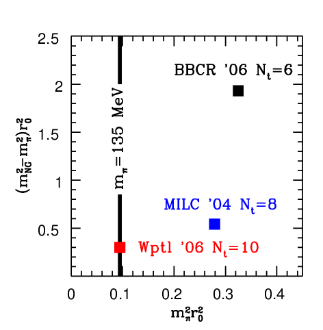
At infinitely large temperatures improved actions (p4 [71] or asqtad [72, 73] action) show considerably smaller discretizations errors, than the standard staggered action (used by this work). However our choice of action is about an order of magnitude faster than e.g. p4, we decided to use this less improved action, with which our CPU resources made it possible to study several lattice spacings ( $N_{t}$ =4 and 6 for the equation of state and $N_{t}=4,6,8$ and $10$ for determining the order of the phase transition and the transition temperature). This turned out to be extremely beneficial, when converting the transition temperature into physical units. In particular the $T=0$ simulations -which are used to do this conversion- have very large lattice artefacts at $N_{t}=4$ and $6$ lattice spacings and can not be used for controlled continuum extrapolations. The high-temperature improvement is not designed to reduce these artefacts.

Setting the physical scale

An additional problem appears if we want to give dimensionful predictions with a few percent accuracy. As we already emphasized lattice QCD predicts dimensionless combinations of physical observables. For dimensionful predictions one calculates an experimentally known dimensionful quantity, which is used then to set the overall scale. In many analyses the overall scale is related to some quantities which strictly speaking do not even exist in full QCD (e.g. the mass of the rho eigenstate and the string tension are not well defined due to decay or string breaking). A better, though still not satisfactory possibility is to use quantities, which are well defined, but can not be measured directly in experiments. Such a quantity is the heavy quark-antiquark potential (V), or its characteristic distances: the $r_{0}$ or $r_{1}$ parameters of V [74] ( $r^{2}d^{2}V/dr^{2}$ =1.65 or 1, for $r_{0}$ or $r_{1}$ , respectively). For these quantities intermediate lattice calculations and/or approximations are needed to connect them to measurements. These calculations are based on bottonium spectroscopy. This procedure leads to further, unnecessary systematic uncertainties.

The ultimate solution is to use quantities, which can be measured directly in experiments and on the lattice. We use the decay constant of the kaon $f_{K}$ =159.8 MeV, which has about 1% measurement error. Detailed additional analyses were done by using the mass of the $K^{*}(892)$ meson $m_{K^{*}}$ , the pion decay constant $f_{\pi}$ and the value of $r_{0}$ , which all show that we are in the $a^{2}$ scaling regime and our choice of overall scale is unambiguous (see subsection 3.1.3).

Algorithm

In previous staggered thermodynamics simulations the inexact R-algorithm was used exclusively to simulate three quark flavours. This algorithm has an intrinsic parameter, the stepsize which, similarly to the lattice spacing, has to be extrapolated to zero. None of the previous staggered lattice thermodynamic studies carried out this extrapolation. Using the R-algorithm without stepsize extrapolation leads to uncontrolled systematic errors. Instead of using the approximate R-algorithm this work uses the exact RHMC-algorithm (rational hybrid Monte-Carlo) [54].

3.4 Order of the QCD transition

The nature of the QCD transition affects our understanding of the Universe’s evolution (see Ref. [75] for example). In a strong first-order phase transition the quark–gluon plasma supercools before bubbles of hadron gas are formed. These bubbles grow, collide and merge, during which gravitational waves could be produced [76]. Baryon-enriched nuggets could remain between the bubbles, contributing to dark matter. The hadronic phase is the initial condition for nucleosynthesis, so inhomogeneities in this phase could have a strong effect on nucleosynthesis [77]. As the first-order phase transition weakens, these effects become less pronounced. Our calculations provide strong evidence that the QCD transition is a crossover and thus the above scenarios —and many others— are ruled out.

There are some QCD results and model calculations to determine the order of the transition at $\mu$ =0 and $\mu$ $\neq$ 0 for different fermionic contents (compare refs [78, 79, 80, 81, 82, 83, 84, 85, 86, 87]). Unfortunately, none of these approaches can give an unambiguous answer for the order of the transition for physical values of the quark masses. The only known systematic technique which could give a final answer is lattice QCD.

There are several lattice results for the order of the QCD transition (for the two most popular lattice fermion formulations see refs [88] and [62]), although they have unknown systematics. As we have already emphasized in the previous section from the lattice point of view there are two important ’ingredients’ to eliminate these systematic uncertainties: one has to use physical quark masses and carry out a continuum extrapolation.

Our goal is to identify the nature of the transition for physical quark masses as we approach the continuum limit. We will study the finite size scaling of the lattice chiral susceptibilities $\chi(N_{s},N_{t})$ = $\partial^{2}$ / $(\partial$ $m_{ud}^{2})$ ( $T/V$ ) $\cdot\log Z$ , where $m_{ud}$ is the mass of the light u,d quarks and $N_{s}$ is the spatial extension. This susceptibility shows a pronounced peak around the transition temperature ( $T_{c}$ ). For a real phase transition the height of the susceptibility peak increases and the width of the peak decreases when we increase the volume. For a first-order phase transition the finite size scaling is determined by the geometric dimension, the height is proportional to $V$ , and the width is proportional to $1/V$ . For a second-order transition the singular behaviour is given by some power of $V$ , defined by the critical exponents. The picture would be completely different for an analytic crossover. There would be no singular behaviour and the susceptibility peak does not get sharper when we increase the volume; instead, its height and width will be $V$ independent for large volumes.

Fig. 3.5 shows the susceptibilities for the light quarks for $N_{t}=$ 4 and 6, for which we used aspect ratios $r=N_{s}/N_{t}$ ranging from 3 to 6 and 3 to 5, respectively. A clear signal for an analytic crossover for both lattice spacings can be seen. However, these curves do not say much about the continuum behaviour of the theory. In principle a phenomenon as unfortunate as that in the three-flavour theory could occur [68], in which the reduction of the discretization effects changed the nature of the transition for a pseudoscalar mass of $\approx$ 140 MeV.

Because we are interested in genuine temperature effects we subtract the $T$ =0 susceptibility and study only the difference between $T$ $\neq$ 0 and $T$ =0 at different lattice spacings. To do it properly, when we approach the continuum limit the renormalization of $\chi$ has to be performed. This leads to $m^{2}$ $\Delta$ $\chi$ , which we study (for the details see subsection 3.5.1).

To give a continuum result for the order of the transition we carry out a finite size scaling analysis of the dimensionless quantity $T^{4}/(m^{2}\Delta\chi)$ directly in the continuum limit. For this study we need the height of the susceptibility peaks in the continuum limit for fixed physical volumes. The continuum extrapolations are done using four different lattice spacings ( $N_{t}$ =4,6,8 and 10). The volumes at different lattice spacings are fixed in units of $T_{c}$ , and thus $VT_{c}^{3}$ = $3^{3}$ , $4^{3}$ and $5^{3}$ were chosen. (In three cases the computer architecture did not allow us to take the above ratios directly. In these cases, we used the next possible volume and interpolated or extrapolated. The height of the peak depends weakly on the volume, so these procedures were always safe.) Altogether we used twelve different lattice volumes ranging from $4\cdot 12^{3}$ to $10\cdot 48^{3}$ at $T>0$ . For the $T=0$ runs lattice volumes from $24\cdot 12^{3}$ up to $56\cdot 28^{3}$ were used. The number of trajectories were between 1500 and 8000 for $T>0$ and between 1500 and 3000 for $T=0$ , respectively. Fig. 3.6 shows the continuum extrapolation for the three different physical volumes. The $N_{t}$ =4 results are slightly off but the $N_{t}$ =6,8 and 10 results show a good $a^{2}$ $\propto$ $1/N_{t}^{2}$ scaling.

Having obtained the continuum values for $T^{4}/(m^{2}\Delta\chi)$ at fixed physical volumes, we study the finite size scaling of the results. Fig. 3.7 shows our final results. The volume dependence strongly suggests that there is no true phase transition but only an analytic crossover in QCD.

3.5 Transition temperature

There are several results in the literature for $T_{c}$ using both staggered and Wilson fermions [89, 90, 62, 91, 64, 66]. There is an additional limitation of these, which has not been mentioned before. This problem is related to an implicit assumption about a a real singularity, thus ignoring the analytic cross-over feature of the finite temperature QCD transition.

As we have seen before the QCD transition at non-vanishing temperatures is an analytic cross-over. Since there is no singular temperature dependence different definitions of the transition point lead to different values. The most famous example for this phenomenon is the water-vapor transition, for which the transition temperature can be defined by the peaks of $d\rho/dT$ (temperature derivative of the density) and $c_{p}$ (heat capacity at fixed pressure). For pressures ( $p$ ) somewhat less than $p_{c}=22.064$ MPa the transition is of first order, whereas at $p=p_{c}$ the transition is second order. In both cases the singularity guarantees that both definitions of the transition temperature lead to the same result. For $p>p_{c}$ the transition is a rapid cross-over, for which e.g. both $d\rho/dT$ and $c_{p}$ show pronounced peaks as a function of the temperature, however these peaks are at different temperature values. Fig. 3.8 shows the phase diagram based on [92]. Analogously, there is no unique transition temperature in QCD.

Our goal is to eliminate all the above limitations and give the full answer. We determine $T_{c}$ using the sharp changes of the temperature (T) dependence of renormalized dimensionless quantities obtained from the chiral condensate ( $\langle\bar{\psi}\psi\rangle$ ), quark number susceptibility ( $n_{q}$ ) and Polyakov loop ( $P$ ). We expect that all three quantities result in different transition points (similarly to the case of the water, c.f. Fig. 3.8).

3.5.1 Chiral susceptibility

The chiral susceptibility of the light quarks ( $\chi$ ) is defined as

\chi_{\bar{\psi}\psi}=\frac{T}{V}\frac{\partial^{2}}{\partial m_{ud}^{2}}\log Z=-\frac{\partial^{2}}{\partial m_{ud}^{2}}f,

(3.5)

where $f$ is the free energy density. Since both the bare quark mass and the free energy density contain divergences, $\chi_{\bar{\psi}\psi}$ has to be renormalized.

The renormalized quark mass can be written as $m_{R,ud}=Z_{m}\cdot m_{ud}$ . If we apply a mass independent renormalization then we have

m_{ud}^{2}\frac{\partial^{2}}{\partial m_{ud}^{2}}=m_{R,ud}^{2}\frac{\partial^{2}}{\partial m_{R,ud}^{2}}.

(3.6)

The free energy has additive, quadratic divergencies. They can be removed by subtracting the free energy at $T=0$ (this is the usual renormalization procedure for the free energy or pressure), which leads to $f_{R}$ . Therefore, we have the following identity:

m_{ud}^{2}\frac{\partial^{2}}{\partial m_{ud}^{2}}\left(f(T)-f(T=0)\right)=m_{R,ud}^{2}\frac{\partial^{2}}{\partial m_{R,ud}^{2}}f_{R}(T).

(3.7)

the right hand side contains only renormalized quantities, which can be determined by measuring the susceptibilities of the left hand side (for the above expression we use the shorthand notation $m_{ud}^{2}\cdot\Delta\chi_{\bar{\psi}\psi}$ ). In order to obtain a dimensionless quantity it is natural to normalize the above quantity by $T^{4}$ (which minimizes the final errors). Alternatively, one can use combinations of $T$ and/or $m_{\pi}$ to construct dimensionless quantities (though these conventions lead to larger errors). Since the transition is a cross-over (c.f. discussion d of our Introduction) the maxima of $m_{ud}^{2}/m_{\pi}^{2}\cdot\Delta\chi_{\bar{\psi}\psi}/T^{2}$ or $m_{ud}^{2}/m_{\pi}^{4}\cdot\Delta\chi_{\bar{\psi}\psi}$ give somewhat different values for $T_{c}$ .

The upper panel of Fig. 3.9 shows the temperature dependence of the renormalized chiral susceptibility for different temporal extensions ( $N_{t}$ =4,6,8 and 10). For small enough lattice spacings, thus close to the continuum limit, these curves should coincide. As it can be seen, the $N_{t}=4$ result has considerable lattice artefacts, however the two smallest lattice spacings ( $N_{t}=8$ and $10$ ) are already consistent with each other, suggesting that they are also consistent with the continuum limit extrapolation (indicated by the orange band). The curves exhibit pronounced peaks. We define the transition temperatures by the position of these peaks. We fitted a second order expression to the peak to obtain its position. The slight change due to the variation of the fitting range is taken as a systematic error. The left panel of Fig. 3.10 shows the transition temperatures in physical units for different lattice spacings obtained from the chiral susceptibility. As it can be seen $N_{t}$ =6,8 and 10 are already in the scaling region, thus a safe continuum extrapolation can be carried out. The extrapolations based on $N_{t}=6,8,10$ fit and $N_{t}=8,10$ fit are consistent with each other. For our final result we use the average of these two fit results (the difference between them are added to our systematic uncertainty). Our T=0 simulations resulted in a $2\%$ error on the overall scale. Our final result for the transition temperature based on the chiral susceptibility reads:

T_{c}(\chi_{\bar{\psi}\psi})=151(3)(3){\rm~MeV},

(3.8)

where the first error comes from the T $\neq$ 0, the second from the T=0 analyses.

We use the second derivative of the chiral susceptibility ( $\chi^{\prime\prime}$ ) at the peak position to estimate the width of the peak ( $(\Delta T_{c})^{2}=-\chi(T_{c})/\chi^{\prime\prime}(T_{c})$ ). For the continuum extrapolated width we obtained:

\Delta T_{c}(\chi_{\bar{\psi}\psi})=28(5)(1){\rm~MeV.}

(3.9)

Note, that for a real phase transition (first or second order), the peak would have a vanishing width (in the thermodynamic limit), yielding a unique value for the transition temperature (which then would be called critical temperature). Due to the crossover nature of the transition there is no such value, there is a range ( $151\pm 28$ MeV) where the transition phenomena takes place. Other quantities than the chiral susceptibility could result in transition temperatures within this range.

The MILC collaboration also reported a continuum result on the transition temperature based on the chiral susceptibility [64]. Their result is 169(12)(4) MeV. Note, that their lattice spacings were not as small as ours (they used $N_{t}$ =4,6 and 8), their aspect ratio was quite small ( $N_{s}$ / $N_{t}$ =2), they used non-physical quark masses (their smallest pion mass at T $\neq$ 0 was $\approx$ 220 MeV), the non-exact R-algorithm was applied for the simulations and they did not use the renormalized susceptibility, but they looked for the peak in the bare $\chi_{\bar{\psi}\psi}/T^{2}$ . Using $T^{4}$ as a normalization prescription (as we did) the transition temperature would decrease their $T_{c}$ values by approximately $9$ MeV. Note, that their continuum extrapolation resulted in a quite large error. Taking into account their uncertainties our result and their result agree on the 1-sigma level.

3.5.2 Quark number susceptibility

For heavy-ion experiments the quark number susceptibilities are quite useful, since they could be related to event-by-event fluctuations. Our second transition temperature is obtained from the strange quark number susceptibility, which is defined via [64]

\frac{\chi_{s}}{T^{2}}=\frac{1}{TV}\left.\frac{\partial^{2}\log Z}{\partial\mu_{s}^{2}}\right|_{\mu_{s}=0},

(3.10)

where $\mu_{s}$ is the strange quark chemical potential (in lattice units). Quark number susceptibilities have the convenient property, that they automatically have a proper continuum limit, there is no need for renormalization.

The middle panel of Fig. 3.9 shows the temperature dependence of the strange quark number susceptibility for different temporal extensions ( $N_{t}$ =4,6,8 and 10). For small enough lattice spacings, thus close to the continuum limit, these curves should coincide again (our continuum limit estimate is indicated by the orange band).

As it can be seen, the $N_{t}=4$ results are quite off, however the two smallest lattice spacings ( $N_{t}=8$ and $10$ ) are already consistent with each other, suggesting that they are also consistent with the continuum limit extrapolation. This feature indicates, that they are closer to the continuum result than our statistical uncertainty.

We defined the transition temperature as the peak in the temperature derivative of the strange quark number susceptibility, that is the inflection point of the susceptibility curve. The position was determined by two independent ways, which yielded the same result. In the first case we fitted a cubic polynomial on the susceptibility curve, while in the second case we determined the temperature derivative numerically from neighboring points and fitted a quadratic expression to the peak. The slight change due to the variation of the fitting range is taken as a systematic error. The middle panel of Fig. 3.10 shows the transition temperatures in physical units for different lattice spacings obtained from the strange quark number susceptibility. As it can be seen $N_{t}$ =6,8 and 10 are already in the $a^{2}$ scaling region, thus a safe continuum extrapolation can be carried out. The extrapolations based on $N_{t}=6,8,10$ fit and $N_{t}=8,10$ fit are consistent with each other. For our final result we use the average of these two fit results (the difference between them is added to our systematic uncertainty). The continuum extrapolated value for the transition temperature based on the strange quark number susceptibility is significantly higher than the one from the chiral susceptibility. The difference is 24(4) MeV. For the transition temperature in the continuum limit one gets:

T_{c}(\chi_{s})=175(2)(4){\rm~MeV},

(3.11)

where the first (second) error is from the T $\neq$ 0 (T=0) temperature analysis (note, that due to the uncertainty of the overall scale, the difference is more precisely determined than the uncertainties of $T_{c}(\chi_{\bar{\psi}\psi})$ and $T_{c}(\chi_{s})$ would suggest). ³³ 3 A continuum extrapolation using only the two coarsest lattices ( $N_{t}=4$ and $6$ ) yielded $T_{c}\sim 190$ MeV [93], where an approximate LCP (LCP1) was used, if the lattice spacing is set by $r_{0}$ . Similarly to the chiral susceptibility analysis, the curvature at the peak can be used to define a width for the transition.

\Delta T_{c}(\chi_{s})=42(4)(1){\rm~MeV}.

(3.12)

3.5.3 Polyakov loop

In pure gauge theory the order parameter of the confinement transition is the Polyakov-loop:

P=\frac{1}{N_{s}^{3}}\sum_{\bf x}{\rm tr}[U_{4}({\bf x},0)U_{4}({\bf x},1)\dots U_{4}({\bf x},N_{t}-1)].

(3.13)

P acquires a non-vanishing expectation value in the deconfined phase, signaling the spontaneous breakdown of the Z(3) symmetry. When fermions are present in the system, the physical interpretation of the Polyakov-loop expectation value is more complicated (see e.g.. [94]). However, its absolute value can be related to the quark-antiquark free energy at infinite separation:

|\langle P\rangle|^{2}=\exp(-\Delta F_{q\bar{q}}(r\to\infty)/T).

(3.14)

$\Delta F_{q\bar{q}}$ is the difference of the free energies of the quark-gluon plasma with and without the quark-antiquark pair.

The absolute value of the Polyakov-loop vanishes in the continuum limit. It needs renormalization. This can be done by renormalizing the free energy of the quark-antiquark pair [95]. Note, that QCD at T $\neq$ 0 has only the ultraviolet divergencies which are already present at T=0. In order to remove these divergencies at a given lattice spacing we used a simple renormalization condition [96]:

V_{R}(r_{0})=0,

(3.15)

where the potential is measured at T=0 from Wilson-loops. The above condition fixes the additive term in the potential at a given lattice spacing. This additive term can be used at the same lattice spacings for the potential obtained from Polyakov loops, or equivalently it can be built in into the definition of the renormalized Polyakov-loop.

|\langle P_{R}\rangle|=|\langle P\rangle|\exp(V(r_{0})/(2T)),

(3.16)

where $V(r_{0})$ is the unrenormalized potential obtained from Wilson-loops.

The lower panel of Fig. 3.9 shows the temperature dependence of the renormalized Polyakov-loops for different temporal extensions ( $N_{t}$ =4,6,8 and 10). The two smallest lattice spacings ( $N_{t}=8$ and $10$ ) are approximately in 1-sigma agreement (our continuum limit estimate is indicated by the orange band).

Similarly to the strange quark susceptibility case we defined the transition temperature as the peak in the temperature derivative of the Polyakov-loop, that is the inflection point of the Polyakov-loop curve. To locate this point and determine its uncertainties we used the same two methods, which were used to determine $T_{c}(\chi_{s})$ . The right panel of Fig. 3.10 shows the transition temperatures in physical units for different lattice spacings obtained from the Polyakov-loop. As it can be seen $N_{t}$ =6,8 and 10 are already in the scaling region, thus a safe continuum extrapolation can be carried out. The extrapolation and the determination of the systematic error were done as for $T_{c}(\chi_{s})$ . The continuum extrapolated value for the transition temperature based on the renormalized Polyakov-loop is significantly higher than the one from the chiral susceptibility. The difference is 25(4) MeV. For the transition temperature in the continuum limit one gets:

T_{c}(P)=176(3)(4){\rm~MeV},

(3.17)

where the first (second) error is from the T $\neq$ 0 (T=0) temperature analysis (again, due to the uncertainties of the overall scale, the difference is more precisely determined than the uncertainties of $T_{c}(\chi)$ and $T_{c}(P)$ suggest). Similarly to the chiral susceptibility analysis, the curvature at the peak can be used to define a width for the transition.

\Delta T_{c}(P)=38(5)(1){\rm~MeV}.

(3.18)

3.5.4 Comparison with the recent result of the BBCR collaboration

Let us comment here on an independent study on $T_{c}$ based on large scale simulations of the Bielefeld-Brookhaven-Columbia-RIKEN group [66]. The p4fat3 action was used, which is designed to give very good results in the (T $\to$ $\infty$ ) Stefan-Boltzmann limit (their action is not optimized at T=0, which is needed e.g. to set the scale). The overall scale was set by $r_{0}$ . The $T_{c}$ analysis based on the chiral susceptibility peak gave in the continuum limit $T_{c}(\chi)$ =192(7)(4) MeV. (The second error, 4 MeV, estimates the uncertainty of the continuum limit extrapolation, which we do not use in the following, since we attempt to give a more reliable estimate on that.) This result is in obvious contradiction with our continuum result from the same observable, which is $T_{c}(\chi)$ =151(3)(3) MeV. For the same quantity (position of chiral susceptibility peak with physical quark masses in the continuum limit) one should obtain the same numerical result independently of the lattice action. Since the chance probability that we are faced with a statistical fluctuation and both of the results are correct is small, we attempted to understand the origin of the discrepancy. We repeated some of their simulations and analyses. In these cases a complete agreement was found. In addition to their T=0 analyses we carried out an $f_{K}$ determination, too. This $f_{K}$ was used to extend their work, to use an LCP based on $f_{K}$ and to determine $T_{c}$ in physical units.

We summarize the origin of the contradiction between our findings and theirs. The major part of the difference can be explained by the fact, that the lattice spacings of [66] are too large ( $\gtrsim$ 0.20 fm), thus they are not in the $a^{2}$ scaling regime, in which a justified continuum extrapolation could have been done. Setting the scale by different dimensionful quantities should lead to the same result. However at their lattice spacings the overall scales obtained by $r_{0}$ or by $f_{K}$ can differ by $\gtrsim$ 20%, and even the continuum extrapolated $r_{0}f_{K}$ value of these scales is about 4–5 $\sigma$ away from the value given by the literature [59, 60]. This scale ambiguity appears in $T_{c}$ , too (though other uncertainties of [66], e.g. coming from the determination of the peak-position, somewhat hide its high statistical significance). We used their $T_{c}$ values fixed by their $r_{0}$ scale, and in addition we converted their peak position of the chiral susceptibility to $T_{c}$ setting the scale by $f_{K}$ . (In order to ensure the possibility of a consistent continuum limit –independently of the actual physical value of $r_{0}$ – we used for both $r_{0}$ and $f_{K}$ the results of [59, 60] as Ref. [66] did it for $r_{0}$ .) Setting the overall scale by $f_{K}$ predicts a much smaller $T_{c}$ at their lattice spacings than doing it by $r_{0}$ (see left panel of Fig. 3.11). Even after carrying out the continuum extrapolation the difference does not vanish ( $\sim 30$ MeV), which means that the lattice spacings $\gtrsim$ 0.20 fm used by [66] are not in the scaling regime. Thus, results obtained with their lattice spacings can not give a consistent continuum limit for $T_{c}$ .

In our case not only $N_{t}=4$ and $6$ temporal extensions were used, but more realistic $N_{t}$ =8 and $10$ simulations were carried out, which led to smaller lattice spacings. These calculations are already in the $a^{2}$ scaling regime and a safe continuum extrapolation can be done. For our lattice spacing different scale setting methods give consistent results. This is shown on the right panel of Fig. 3.11 (independently of the scale setting one obtains the same $T_{c}$ ) and also justified with high accuracy by Fig. 3.3, where $r_{0}f_{K}$ converges to the physical value on our finer lattices. As it can be seen on the plot, using only our $N_{t}=4$ and 6 results would also give an inconsistent continuum limit. This emphasizes our conclusion that lattice spacings $\gtrsim$ 0.20 fm can not be used for consistent continuum extrapolations.

The second, minor part of the difference comes from the different definitions of the transition temperatures related to the chiral susceptibility. We use the renormalized chiral susceptibility with $T^{4}$ normalization to obtain the peak position, which yields $\sim 9$ MeV smaller transition temperature than the bare susceptibility normalized by $T^{2}$ of Ref. [66].

3.6 Equation of state

The equilibrium description as a function of the temperature is given by the equation of state (EoS). The complete determination of the EoS needs non-perturbative inputs, out of which the lattice simulation is the most systematic approach.

The EoS has been determined in the continuum limit for the pure gauge theory [97, 98, 99]. In this case –quenched simulations– the simulations are particularly easy as there is no fermionic degree of freedom. The simulated systems is equivalent to that where all the fermions are infinitely heavy, thus, is far from the physical situation. (Note, however, that even in this relatively simple case there is still a few % difference between the different approaches.)

The situation in the unquenched case (QCD with dynamical quarks) is a bit barouqe. There are many results with different flavor content, fermion formulation, quark masses. None of them have used the proper physical quark content and none of them has attempted to carry out a continuum extrapolation. Moreover staggered fermion studies were always using inexact R-algorithm (which can result in uncontrolled systematics, see subsection 3.1.2). Let us give here a brief review of the literature.

•

There are published results for two-flavor QCD using unimproved staggered [100, 101], and improved Wilson fermions [63].
•

There are results available for the 2+1 flavour case, among which the study done by Karsch, Laermann and Peikert in the year 2000 [102], using p4-improved staggered fermions, has often been used as the best result of EoS from lattice QCD. An additional drawback of this result, that the concept of the LCP was ignored from the calculation. If Karsch,Laermann and Peikert had cooled down e.g. two of their systems one at $T$ =3 $T_{c}$ and one at $T$ =0.7 $T_{c}$ down to T=0, the first system would have had approximately 4 times larger quark masses -two times larger pion masses- than the second one; this unphysical choice is known to lead systematics, which are comparable to the difference between the interacting and non-interacting plasma
•

Recently the MILC collaboration studied the equation of state along LCP’s with two light quark masses (0.1 and 0.2 times $m_{s}$ ) at $N_{t}$ =4 and 6 lattices using asqtad improved staggered fermionic action [65].

There are ongoing thermodynamics projects improving on previous results. The joint Bielefeld-Brookhaven-Columbia-MILC-RIKEN collaboration (hotQCD collaboration) have presented new results at the lattice conference [103]. Still the results are only available for two different lattice spacings ( $N_{t}=4$ and $6$ ) and for unphyiscal quark masses.

There are two important further issues with the equation of state, which have been overlooked in previous calculations. Firstly the heavier quarks can have significant contribution to the pressure even at few times the transition temperature (exploratory investigations [104] show a significant jump in the pressure around $\sim 2\cdot T_{c}$ due to the charm quark). Secondly there is no serious practical obstacle to extend the EoS calculations well beyond the usual $4-5\cdot T_{c}$ [105]. This opens the possibility to find the missing connection between conventional perturbation theory and nonperturbative methods.

In this section we present our first step towards the final solution of the EoS with proper physical quark content. Though we have the EoS on two different sets of lattice spacings ( $N_{t}=4$ and $6$ ) and one might attempt to do a continuum extrapolation, it is fair to say that another set of lattice spacings is needed ( $N_{t}$ =8). One of the reasons is, that in the hadronic phase, where the integration for the pressure starts, the lattice spacing is larger than 0.3 fm. In this region the lattice artefacts can not be really controlled (and in this deeply hadronic case it does not really help that an action is very good at asymptotically high temperatures in the free non-interacting gas limit).

3.6.1 Integral technique

We shortly review the integral technique to obtain the pressure [106]. For large homogeneous systems the pressure is proportional to the logarithm of the partition function:

\displaystyle pa^{4}=\frac{Ta}{V/a^{3}}\log Z(T,V)=\frac{1}{N_{t}N_{s}^{3}}\log Z(N_{s},N_{t};\beta,m_{q}).

(3.19)

(Index ‘q’ refers to the ${ud}$ and $s$ flavors.) The volume and temperature are connected to the spatial and temporal extensions of the lattice:

\displaystyle V=(N_{s}a)^{3},

\displaystyle T=\frac{1}{N_{t}a}.

(3.20)

The divergent zero-point energy has to be removed by subtracting the zero temperature ( $N_{t}\to\infty$ ) part of Eq. (3.19). In practice the zero temperature subtraction is performed by using lattices with finite, but large $N_{t}$ (called $N_{t0}$ , see Table 3.1). So the normalized pressure becomes:

\displaystyle\frac{p}{T^{4}}=N_{t}^{4}\left[\frac{1}{N_{t}N_{s}^{3}}\log Z(N_{s},N_{t};\beta,m_{q})-\frac{1}{N_{t0}N_{s0}^{3}}\log Z(N_{s0},N_{t0};\beta,m_{q})\right].

(3.21)

With usual Monte-Carlo techniques one cannot measure $\log Z$ directly, but only its derivatives with respect to the bare parameters of the lattice action. Having determined the partial derivatives one integrates in the multi-dimensional parameter space:

\frac{p}{T^{4}}=N_{t}^{4}\int^{(\beta,m_{q})}_{(\beta_{0},m_{q0})}d(\beta,m_{q})\left[\frac{1}{N_{t}N_{s}^{3}}\left(\begin{array}[]{c}{\partial\log Z}/{\partial\beta}\\ {\partial\log Z}/{\partial m_{q}}\end{array}\right)-\frac{1}{N_{t0}N_{s0}^{3}}\left(\begin{array}[]{c}{\partial\log Z_{0}}/{\partial\beta}\\ {\partial\log Z_{0}}/{\partial m_{q}}\end{array}\right)\right],

(3.22)

where $Z/Z_{0}$ are shorthand notations for $Z(N_{s},N_{t})/Z(N_{s0},N_{t0})$ . Since the integrand is a gradient, the result is by definition independent of the integration path. We need the pressure along the LCP, thus it is convenient to measure the derivatives of $\log Z$ along the LCP and perform the integration over this line in the $\beta$ , $m_{ud}$ and $m_{s}$ parameter space. The lower limits of the integrations (indicated by $\beta_{0}$ and $m_{q0}$ ) were set sufficiently below the transition point. By this choice the pressure gets independent of the starting point (in other words it vanishes at small temperatures). In the case of $2+1$ flavor staggered QCD the derivatives of $\log Z$ with respect to $\beta$ and $m_{q}$ are proportional to the expectation value of the gauge action ( $\langle S_{g}\rangle$ c.f. Eq. (3.1)) and to the chiral condensates ( $\langle\bar{\psi}\psi_{q}\rangle$ ), respectively. Eq. (3.22) can be rewritten appropriately and the pressure is given by (in this formula we write out explicitely the flavors):

\frac{p}{T^{4}}=N_{t}^{4}\int^{(\beta,m_{ud},m_{s})}_{(\beta_{0},m_{ud0},m_{s0})}d(\beta,m_{ud},m_{s})\left[\frac{1}{N_{t}N_{s}^{3}}\left(\begin{array}[]{c}\langle{\rm-S_{g}/\beta}\rangle\\ \langle\bar{\psi}\psi_{ud}\rangle\\ \langle\bar{\psi}\psi_{s}\rangle\end{array}\right)-\frac{1}{N_{t0}N_{s0}^{3}}\left(\begin{array}[]{c}\langle{\rm-S_{g}/\beta}\rangle_{0}\\ \langle\bar{\psi}\psi_{ud}\rangle_{0}\\ \langle\bar{\psi}\psi_{s}\rangle_{0}\end{array}\right)\right],

(3.23)

where $\langle\dots\rangle_{0}$ means averaging on a $N_{s0}^{3}\cdot N_{t0}$ lattice.

The integral method was originally introduced for the pure gauge case, for which the integral is one dimensional, it is performed along the $\beta$ axis. Many previous studies for staggered dynamical QCD (e.g. [101, 107, 102]) used a one-dimensional parameter space instead of performing it along the LCP. Note, that for full QCD the integration should be performed along a LCP path in a multi-dimensional parameter space.

$N_{t}$	p/ $T^{4}$	$c_{s}^{2}$	$\chi/T^{2}$
4	9.12	1/3	2.24
6	7.86	1/3	1.86
$\infty$	5.21	1/3	1

Table 3.4: Summary of the results for the 2+1 flavor pressure, speed of sound and 1 flavor quark number susceptibility in the non-interacting Stefan-Boltzmann limit.

\epsilon/T^{4}

is 3 times, whereas

s/T^{3}

is 4 times the normalized value of the pressure (

p/T^{4}

) in the Stefan-Boltzmann limit. The first two lines gives the results for

N_{t}

=4,6 and the third line contains the results in the continuum (in the thermodynamic limit).

Using appropriate thermodynamical relations one can obtain any thermal properties of the system. For example the energy density ( $\epsilon$ ), entropy density ( $s$ ) and speed of sound ( $c_{s}^{2}$ ) can be derived as

\displaystyle\epsilon=T(\partial p/\partial T)-p,

\displaystyle s=(\epsilon+p)T,

\displaystyle c_{s}^{2}=\frac{dp}{d\epsilon}.

(3.24)

To be able to do theses derivatives one has to know the temperature along the LCP. Since the temperature is connected to the lattice spacing as $T=(N_{t}a)^{-1},$ we need a reliable estimate on $a$ . The lattice spacings at different points of the LCP are determined by first matching the static potentials for different $\beta$ values at an intermediate distance for $m_{ud}=\{3,5\}m_{ud}(phys)$ quark masses, then extrapolating the results to the physical quark mass. Relating these distances to physical observables (determining the overall scale in physical units) will be the topic of a subsequent publication. We show the results as a function of $T/T_{c}$ . The transition temperature ( $T_{c}$ ) is defined by the inflection point of the isospin number susceptibility ( $\chi_{I}$ , see later).

To get the energy density the literature usually uses another quantity, namely $\epsilon$ -3 $p$ , which can be also directly measured on the lattice. In our analysis it turned out to be more appropriate to calculate first the pressure directly from the raw lattice data (Eq. (3.23)) and then determine the energy density and other quantities from the pressure (Eq. (3.24)). The reasons for that can be summarized as follows. As we discussed we perform T $\neq$ 0 simulations with physical quark masses, whereas the subtraction terms from T=0 simulations are extrapolated from larger quark masses. This sort of extrapolation is adequate for the chiral condensates, for which chiral perturbation techniques work well. Thus, one can choose an integration path for the T=0 part of the pressure, which moves along a LCP at some larger $m_{ud}$ (e.g. 9 times $m_{ud}(phys)$ ) and then at fixed $\beta$ goes down to the physical quark mass. No comparable analogous technique is available for the combination $\epsilon$ -3 $p$ .

We have also calculated the pressure for the larger quark masses. Plotting it as a function of the temperature the differences between them are significant. As a function of $T/T_{c}$ these differences are smaller, but still remain statistically significant in the $1.2...2.0T_{c}$ region. Note that statements on the mass dependence are only qualitative since such an analysis requires the careful matching of the scales at different quark masses.

3.6.2 Physics results

$\beta$	$T/T_{c}$	$p/T^{4}$ (raw)	$p/T^{4}$ (scaled)	$\beta$	$T/T_{c}$	$p/T^{4}$ (raw)	$p/T^{4}$ (scaled)
3.000	$0.90$	$0.12(0.02)$	$0.07(0.01)$	3.450	$0.80$	$0.07(0.11)$	$0.05(0.08)$
3.150	$0.95$	$0.32(0.07)$	$0.19(0.04)$	3.500	$0.87$	$0.23(0.11)$	$0.15(0.08)$
3.250	$0.98$	$0.59(0.10)$	$0.34(0.06)$	3.550	$0.96$	$0.59(0.12)$	$0.39(0.08)$
3.275	$0.99$	$0.73(0.10)$	$0.42(0.06)$	3.575	$1.02$	$0.91(0.12)$	$0.60(0.08)$
3.300	$1.01$	$0.91(0.10)$	$0.52(0.06)$	3.600	$1.07$	$1.29(0.13)$	$0.86(0.08)$
3.325	$1.04$	$1.13(0.10)$	$0.65(0.06)$	3.625	$1.14$	$1.69(0.13)$	$1.12(0.09)$
3.350	$1.06$	$1.39(0.09)$	$0.79(0.05)$	3.650	$1.20$	$2.10(0.14)$	$1.40(0.09)$
3.400	$1.14$	$2.04(0.10)$	$1.16(0.06)$	3.675	$1.28$	$2.51(0.14)$	$1.66(0.10)$
3.450	$1.23$	$2.79(0.10)$	$1.59(0.06)$	3.700	$1.35$	$2.88(0.15)$	$1.91(0.10)$
3.500	$1.34$	$3.56(0.11)$	$2.04(0.07)$	3.750	$1.52$	$3.50(0.15)$	$2.32(0.10)$
3.550	$1.49$	$4.32(0.12)$	$2.47(0.07)$	3.800	$1.70$	$3.99(0.16)$	$2.65(0.11)$
3.600	$1.66$	$4.96(0.12)$	$2.83(0.07)$	3.850	$1.90$	$4.36(0.16)$	$2.89(0.11)$
3.650	$1.86$	$5.46(0.12)$	$3.12(0.07)$	3.930	$2.24$	$4.82(0.17)$	$3.19(0.11)$
3.700	$2.09$	$5.84(0.12)$	$3.34(0.07)$	4.000	$2.55$	$5.14(0.17)$	$3.41(0.11)$
3.850	$2.93$	$6.57(0.15)$	$3.75(0.09)$
4.000	$3.93$	$6.97(0.16)$	$3.98(0.09)$

Table 3.5: Numerical values of the pressure for all of our simulation points. The left column shows the

N_{t}

=4, whereas the right column shows the

N_{t}

=6 data. Both the raw values and the ones scaled by

c_{cont}/c_{N_{t}}

are given.

Let us present the results. In order to show how the different quantities scale with the lattice spacing we show always $N_{t}$ =4,6 results on the same plot. In addition, in order to make the relationship with the continuum limit more transparent we multiply the raw lattice results at finite temporal extensions ( $N_{t}$ =4,6) with $c_{cont}/c_{N_{t}}$ , where the c values are the results in the free non-interacting plasma (Stefan-Boltzmann limit). These c values are summarized in Table 3.4 for the pressure, speed of sound, and for the quark number susceptibility at $N_{t}$ =4,6 and in the continuum limit. By this multiplication the lattice thermodynamic quantities should approach the continuum Stefan-Boltzmann values for extreme large temperatures.

Table 3.5 contains our most important numerical results. We tabulated the raw and normalized pressure values for both lattice spacings and for all of our simulation points. This data set and Eq. (3.24) were used to obtain the following figures. Fig. 3.12 shows the equation of state on $N_{t}$ =4,6 lattices. The pressure (left panel) and $\epsilon$ (right panel) are presented as a function of the temperature. The Stefan-Boltzmann limit is also shown. Fig. 3.13 shows the entropy density (left panel) and the speed of sound (right panel), which can be obtained by using the pressure and energy density data (c.f. $sT$ = $\epsilon$ + $p$ and $c_{s}^{2}$ = $dp$ / $d\epsilon$ ) of the previous Fig. 3.12. Clearly, the uncertainties of the pressure and those of the energy density cumulate in the speed of sound, therefore it is less precisely determined.

Light and strange quark number susceptibilities ( $\chi_{ud}$ and $\chi_{s}$ ) are defined via [64]

\displaystyle\frac{\chi_{q}}{T^{2}}=\frac{N_{t}}{N_{s}^{3}}\left.\frac{\partial^{2}\log Z}{\partial\mu_{q}^{2}}\right|_{\mu_{q}=0},

(3.25)

where $\mu_{ud}$ and $\mu_{s}$ are the light and strange quark chemical potentials (in lattice units). With the help of the quark number operators

Q_{q}=\frac{1}{4}\frac{\partial}{\partial\mu_{q}}\log\det({D\hskip-7.0pt{/}}+m_{q}),

the susceptibilities can be written as

\frac{\chi_{q}}{T^{2}}=\frac{N_{t}}{N_{s}^{3}}\left(\langle Q_{q}^{2}\rangle_{\mu_{q}=0}+\left\langle\frac{\partial Q_{q}}{\partial\mu_{q}}\right\rangle_{\mu_{q}=0}\right).

The first term is usually referred as disconnected, the second as connected part. The connected part of the light quark number susceptibility is 2 times the susceptibility of the isospin number ( $\chi_{I}$ ). It is presented on the left panel of Fig. 3.13. For our statistics and evaluation method the disconnected parts are all consistent with zero and their value is far smaller than those of the connected parts. The right panel of Fig. 3.13 contains the connected part of the strange number susceptibility.

Chapter 4 Summary

The focus of this work was implementing and applying dynamical fermions in lattice QCD.

The first part was exploring the unknown territory of dynamical algorithms for the overlap fermion. The conventional dynamical algorithm (Hybrid Monte Carlo) fails to work for this type of fermion. The failure was identified, it is due to the change in the topological charge. We have proposed a possible workaround for this problem, and shown that with this modification the algorithm works reasonably. There were further modifications necessary to increase the performance to an acceptable level. At the end we have determined the topological susceptibility as the function of quark mass. The result was the first in lattice QCD which has shown the suppression of the susceptibility for small quark masses at finite lattice spacing. The simulations however considerably more expensive than the ones with other fermion formulations. Therefore it still seems to be more beneficial to investigate the current algorithms or to come up with new ones than starting larger scale physics projects with dynamical overlap fermions.

The second part of the work was the determination of bulk properties of the finite temperature QCD matter using dynamical improved staggered fermions. This was a large scale project and attempted to give final answers based on a first principles approach. In order to achieve our goal we have done the simulations for physical values of the quark masses and carried out a continuum extrapolation wherever possible. Firstly we have determined the nature of the transition based on a finite size scaling analysis of a susceptibility type quantity. The transition turned out to be a smooth crossover, that is no sign of singularity has been found in the thermodynamical limit. Secondly we have determined some typical temperatures in physical units where this crossover takes place. Since there is no singularity, there is no unique temperature which can be identified as a critical temperature. We have calculated transition temperatures from various quantities: peak of the chiral susceptibility, inflection point of the quark number susceptibility and inflection point of the Polyakov loop. The second two gave significantly higher temperature values, than the first one. Thirdly we have presented result on the equation of state towards the continuum limit. From the currently available lattice spacings a reliable continuum extrapolation cannot be carried out, this is left for the future.

Acknowledgments

First of all I would like to thank the help of my advisor Zoltán Fodor. His very good sense in choosing the right topics was inevitable to accomplish this thesis. I am also very grateful to Sándor Katz. They both have a great part in my results with lots of ideas, hints.

In the overlap project we had a nice collaboration with Győző Egri, I thank him. It was a pleasure to work together at various stages of the staggered project with Yasumichi Aoki and Gergő Endrődi. I thank the discussions with Christian Hoelbling, Dániel Nógrádi, Stefan Krieg, Tamás Kovács, Anna Tóth and Bálint Tóth.

The numerical computations for this thesis were carried out on the following supercomputers: on BlueGene/L at FZ Jülich, on PC clusters at Bergische Universität, Wuppertal and on PC clusters at Eötvös University, Budapest.

Bibliography

[1] I. Montvay and G. Munster. Quantum fields on a lattice. Cambridge, UK: Univ. Pr. (1994) 491 p. (Cambridge monographs on mathematical physics).
[2] Rajan Gupta. Introduction to lattice qcd. 1997.
[3] H. J. Rothe. Lattice gauge theories: An introduction. World Sci. Lect. Notes Phys., 74:1–605, 2005.
[4] J. Berges, Sz. Borsanyi, D. Sexty, and I. O. Stamatescu. Lattice simulations of real-time quantum fields. Phys. Rev., D75:045007, 2007.
[5] Stephen R. Sharpe. Rooted staggered fermions: Good, bad or ugly? PoS, LAT2006:022, 2006.
[6] Stephan Durr and Christian Hoelbling. Staggered versus overlap fermions: A study in the schwinger model with n(f) = 0,1,2. Phys. Rev., D69:034503, 2004.
[7] L. Del Debbio, L. Giusti, M. Luscher, R. Petronzio, and N. Tantalo. Stability of lattice qcd simulations and the thermodynamic limit. JHEP, 02:011, 2006.
[8] Z. Fodor, S. D. Katz, and K. K. Szabo. Dynamical overlap fermions, results with hybrid monte-carlo algorithm. JHEP, 08:003, 2004.
[9] G. I. Egri, Z. Fodor, S. D. Katz, and K. K. Szabo. Topology with dynamical overlap fermions. JHEP, 01:049, 2006.
[10] Y. Aoki, G. Endrodi, Z. Fodor, S. D. Katz, and K. K. Szabo. The order of the quantum chromodynamics transition predicted by the standard model of particle physics. Nature, 443:675–678, 2006.
[11] Y. Aoki, Z. Fodor, S. D. Katz, and K. K. Szabo. The qcd transition temperature: Results with physical masses in the continuum limit. Phys. Lett., B643:46–54, 2006.
[12] Y. Aoki, Z. Fodor, S. D. Katz, and K. K. Szabo. The equation of state in lattice qcd: With physical quark masses towards the continuum limit. JHEP, 01:089 [16 pages], 2006.
[13] Paul H. Ginsparg and Kenneth G. Wilson. A remnant of chiral symmetry on the lattice. Phys. Rev., D25:2649, 1982.
[14] Peter Hasenfratz. Lattice qcd without tuning, mixing and current renormalization. Nucl. Phys., B525:401–409, 1998.
[15] Herbert Neuberger. Vector like gauge theories with almost massless fermions on the lattice. Phys. Rev., D57:5417–5433, 1998.
[16] Ferenc Niedermayer. Exact chiral symmetry, topological charge and related topics. Nucl. Phys. Proc. Suppl., 73:105–119, 1999.
[17] Martin Luscher. Exact chiral symmetry on the lattice and the ginsparg- wilson relation. Phys. Lett., B428:342–345, 1998.
[18] Thomas A. DeGrand. A variant approach to the overlap action. Phys. Rev., D63:034503, 2001.
[19] Christof Gattringer et al. Quenched spectroscopy with fixed-point and chirally improved fermions. Nucl. Phys., B677:3–51, 2004.
[20] Ronald Babich et al. Light hadron and diquark spectroscopy in quenched qcd with overlap quarks on a large lattice. JHEP, 01:086, 2006.
[21] Herbert Neuberger. Exactly massless quarks on the lattice. Phys. Lett., B417:141–144, 1998.
[22] Herbert Neuberger. More about exactly massless quarks on the lattice. Phys. Lett., B427:353–355, 1998.
[23] Peter Hasenfratz, Victor Laliena, and Ferenc Niedermayer. The index theorem in qcd with a finite cut-off. Phys. Lett., B427:125–131, 1998.
[24] Anna Hasenfratz, Peter Hasenfratz, and Ferenc Niedermayer. Simulating full qcd with the fixed point action. Phys. Rev., D72:114508, 2005.
[25] Robert G. Edwards, Urs M. Heller, and Rajamani Narayanan. A study of practical implementations of the overlap-dirac operator in four dimensions. Nucl. Phys., B540:457–471, 1999.
[26] J. van den Eshof, A. Frommer, T. Lippert, K. Schilling, and H. A. van der Vorst. Numerical methods for the qcd overlap operator. i: Sign- function and error bounds. Comput. Phys. Commun., 146:203–224, 2002.
[27] T. Struckmann et al. Flavor singlet pseudoscalar masses in n(f) = 2 qcd. Phys. Rev., D63:074503, 2001.
[28] Ting-Wai Chiu, Tung-Han Hsieh, Chao-Hsi Huang, and Tsung-Ren Huang. A note on the zolotarev optimal rational approximation for the overlap dirac operator. Phys. Rev., D66:114502, 2002.
[29] Andreas Frommer, Bertold Nockel, Stephan Gusken, Thomas Lippert, and Klaus Schilling. Many masses on one stroke: Economic computation of quark propagators. Int. J. Mod. Phys., C6:627–638, 1995.
[30] Beat Jegerlehner. Krylov space solvers for shifted linear systems. 1996.
[31] Gyozo I. Egri et al. Lattice qcd as a video game. Comput. Phys. Commun., 177:631–639, 2007.
[32] S. Duane, A. D. Kennedy, B. J. Pendleton, and D. Roweth. Hybrid monte carlo. Phys. Lett., B195:216–222, 1987.
[33] Guido Arnold et al. Numerical methods for the qcd overlap operator. ii: Optimal krylov subspace methods. 2003.
[34] Rajamani Narayanan and Herbert Neuberger. An alternative to domain wall fermions. Phys. Rev., D62:074504, 2000.
[35] Nigel Cundy et al. Numerical methods for the qcd overlap operator. iii: Nested iterations. Comput. Phys. Commun., 165:221–242, 2005.
[36] Thomas A. DeGrand and Stefan Schaefer. Physics issues in simulations with dynamical overlap fermions. Phys. Rev., D71:034507, 2005.
[37] N. Cundy et al. Numerical methods for the qcd overlap operator. iv: Hybrid monte carlo. hep-lat/0502007, 2005.
[38] Stefan Schaefer and Thomas A. DeGrand. Dynamical overlap fermions: Techniques and results. simulations and physics results. PoS, LAT2005:140, 2006.
[39] Achim Bode, Urs M. Heller, Robert G. Edwards, and Rajamani Narayanan. First experiences with hmc for dynamical overlap fermions. 1999.
[40] Thomas DeGrand and Stefan Schaefer. Simulating an arbitrary number of flavors of dynamical overlap fermions. JHEP, 07:020, 2006.
[41] Thomas A. DeGrand, Anna Hasenfratz, and Tamas G. Kovacs. Improving the chiral properties of lattice fermions. Phys. Rev., D67:054501, 2003.
[42] Tamas G. Kovacs. Locality and topology with fat link overlap actions. Phys. Rev., D67:094501, 2003.
[43] Colin Morningstar and Mike J. Peardon. Analytic smearing of su(3) link variables in lattice qcd. Phys. Rev., D69:054501, 2004.
[44] Martin Luscher. Abelian chiral gauge theories on the lattice with exact gauge invariance. Nucl. Phys., B549:295–334, 1999.
[45] David H. Adams. Gauge fixing, families index theory, and topological features of the space of lattice gauge fields. Nucl. Phys., B640:435–452, 2002.
[46] Steven A. Gottlieb, W. Liu, D. Toussaint, R. L. Renken, and R. L. Sugar. Hybrid molecular dynamics algorithms for the numerical simulation of quantum chromodynamics. Phys. Rev., D35:2531–2542, 1987.
[47] Z. Fodor, S. D. Katz, and K. K. Szabo. Dynamical overlap fermions, results with hmc algorithm. Nucl. Phys. Proc. Suppl., 140:704–706, 2005.
[48] Stephan Durr, Christian Hoelbling, and Urs Wenger. Filtered overlap: Speedup, locality, kernel non-normality and z(a) approx. 1. JHEP, 09:030, 2005.
[49] Ting-Wai Chiu, Tung-Han Hsieh, Chao-Hsi Huang, and Tsung-Ren Huang. A computational system for lattice qcd with overlap dirac quarks. Nucl. Phys. Proc. Suppl., 119C:1050–1052, 2003.
[50] A. D. Kennedy and Pietro Rossi. Classical mechanics on group manifolds and applications to hybrid monte carlo. Nucl. Phys., B327:782, 1989.
[51] Z. Fodor and S. D. Katz. A new method to study lattice qcd at finite temperature and chemical potential. Phys. Lett., B534:87–92, 2002.
[52] Z. Fodor and S. D. Katz. Lattice determination of the critical point of qcd at finite t and mu. JHEP, 03:014, 2002.
[53] Christian Schmidt. Lattice qcd at finite density. PoS, LAT2006:021, 2006.
[54] M. A. Clark and A. D. Kennedy. The rhmc algorithm for 2 flavors of dynamical staggered fermions. Nucl. Phys. Proc. Suppl., 129:850–852, 2004.
[55] Roberto Frezzotti and Karl Jansen. A polynomial hybrid monte carlo algorithm. Phys. Lett., B402:328–334, 1997.
[56] M. A. Clark and A. D. Kennedy. Accelerating dynamical fermion computations using the rational hybrid monte carlo (rhmc) algorithm with multiple pseudofermion fields. 2006.
[57] Zoltan Fodor, Sandor D. Katz, and Gabor Papp. Better than 1 usd/mflops sustained: A scalable pc-based parallel computer for lattice qcd. Comput. Phys. Commun., 152:121–134, 2003.
[58] F. Csikor et al. Equation of state at finite temperature and chemical potential, lattice qcd results. JHEP, 05:046, 2004.
[59] C. Aubin et al. Light pseudoscalar decay constants, quark masses, and low energy constants from three-flavor lattice qcd. Phys. Rev., D70:114501, 2004.
[60] A. Gray et al. The upsilon spectrum and m(b) from full lattice qcd. Phys. Rev., D72:094507, 2005.
[61] Gilberto Colangelo, Stephan Durr, and Christoph Haefeli. Finite volume effects for meson masses and decay constants. Nucl. Phys., B721:136–174, 2005.
[62] A. Ali Khan et al. Phase structure and critical temperature of two flavor qcd with renormalization group improved gauge action and clover improved wilson quark action. Phys. Rev., D63:034502 [11 pages], 2001.
[63] A. Ali Khan et al. Equation of state in finite-temperature qcd with two flavors of improved wilson quarks. Phys. Rev., D64:074510, 2001.
[64] C. Bernard et al. Qcd thermodynamics with three flavors of improved staggered quarks. Phys. Rev., D71:034504, 2005.
[65] C. Bernard et al. Qcd equation of state with 2+1 flavors of improved staggered quarks. Phys. Rev., D75:094505, 2007.
[66] M. Cheng et al. The transition temperature in qcd. Phys. Rev., D74:054507, 2006.
[67] Satchidananda Naik. On-shell improved lattice action for qcd with susskind fermions and asymptotic freedom scale. Nucl. Phys., B316:238, 1989.
[68] F. Karsch et al. Where is the chiral critical point in 3-flavor qcd? Nucl. Phys. Proc. Suppl., 129:614–616, 2004.
[69] G. Endrodi. Lattice 2007 talk.
[70] O. Philipsen. Lattice 2007 talk.
[71] Urs M. Heller, F. Karsch, and B. Sturm. Improved staggered fermion actions for qcd thermodynamics. Phys. Rev., D60:114502, 1999.
[72] G. Peter Lepage. Flavor-symmetry restoration and symanzik improvement for staggered quarks. Phys. Rev., D59:074502, 1999.
[73] Kostas Orginos, Doug Toussaint, and R. L. Sugar. Variants of fattening and flavor symmetry restoration. Phys. Rev., D60:054503, 1999.
[74] R. Sommer. A new way to set the energy scale in lattice gauge theories and its applications to the static force and alpha-s in su(2) yang-mills theory. Nucl. Phys., B411:839–854, 1994.
[75] Dominik J. Schwarz. The first second of the universe. Annalen Phys., 12:220–270, 2003.
[76] Edward Witten. Cosmic separation of phases. Phys. Rev., D30:272–285, 1984.
[77] J. H. Applegate and C. J. Hogan. Relics of cosmic quark condensation. Phys. Rev., D31:3037–3045, 1985.
[78] Robert D. Pisarski and Frank Wilczek. Remarks on the chiral phase transition in chromodynamics. Phys. Rev., D29:338–341, 1984.
[79] T. Celik, J. Engels, and H. Satz. The order of the deconfinement transition in su(3) yang- mills theory. Phys. Lett., B125:411–414, 1983.
[80] John B. Kogut et al. Deconfinement and chiral symmetry restoration at finite temperatures in su(2) and su(3) gauge theories. Phys. Rev. Lett., 50:393–396, 1983.
[81] Steven A. Gottlieb et al. The deconfining phase transition and the continuum limit of lattice quantum chromodynamics. Phys. Rev. Lett., 55:1958–1961, 1985.
[82] F. R. Brown, N. H. Christ, Y. F. Deng, M. S. Gao, and T. J. Woch. Nature of the deconfining phase transition in su(3) lattice gauge theory. Phys. Rev. Lett., 61:2058–2061, 1988.
[83] M. Fukugita, M. Okawa, and A. Ukawa. Order of the deconfining phase transition in su(3) lattice gauge theory. Phys. Rev. Lett., 63:1768–1771, 1989.
[84] M. A. Halasz, A. D. Jackson, R. E. Shrock, Misha A. Stephanov, and J. J. M. Verbaarschot. On the phase diagram of QCD. Phys. Rev., D58:096007 [11 pages], 1998.
[85] Jurgen Berges and Krishna Rajagopal. Color superconductivity and chiral symmetry restoration at nonzero baryon density and temperature. Nucl. Phys., B538:215–232, 1999.
[86] Bernd-Jochen Schaefer and Jochen Wambach. The phase diagram of the quark meson model. Nucl. Phys., A757:479–492, 2005.
[87] T. Herpay, A. Patkos, Zs. Szep, and P. Szepfalusy. Mapping the boundary of the first order finite temperature restoration of chiral symmetry in the (m(pi) - m(k))-plane with a linear sigma model. Phys. Rev., D71:125017 [15 pages], 2005.
[88] Frank R. Brown et al. On the existence of a phase transition for qcd with three light quarks. Phys. Rev. Lett., 65:2491–2494, 1990.
[89] F. Karsch, E. Laermann, and A. Peikert. Quark mass and flavor dependence of the qcd phase transition. Nucl. Phys., B605:579–599, 2001.
[90] Claude W. Bernard et al. Qcd thermodynamics with an improved lattice action. Phys. Rev., D56:5584–5595, 1997.
[91] V. G. Bornyakov et al. Finite temperature qcd with two flavors of non- perturbatively improved wilson fermions. Phys. Rev., D71:114504, 2005.
[92] Bernhard Spang. http://www.cheresources.com/iapwsif97.shtml.
[93] S. D. Katz. Equation of state from lattice qcd. http://qm2005.kfki.hu/talk2_select.pshtml?sel=27.
[94] Slavo Kratochvila and Philippe de Forcrand. Qcd at zero baryon density and the polyakov loop paradox. Phys. Rev., D73:114512, 2006.
[95] O. Kaczmarek, F. Karsch, P. Petreczky, and F. Zantow. Heavy quark anti-quark free energy and the renormalized polyakov loop. Phys. Lett., B543:41–47, 2002.
[96] Z. Fodor, S. D. Katz, K. K. Szabo, and A. I. Toth. Grand canonical potential for a static quark anti-quark pair at mu not equal 0. Nucl. Phys. Proc. Suppl., 140:508–510, 2005.
[97] G. Boyd et al. Thermodynamics of su(3) lattice gauge theory. Nucl. Phys., B469:419–444, 1996.
[98] M. Okamoto et al. Equation of state for pure su(3) gauge theory with renormalization group improved action. Phys. Rev., D60:094510, 1999.
[99] Y. Namekawa et al. Thermodynamics of su(3) gauge theory on anisotropic lattices. Phys. Rev., D64:074507, 2001.
[100] T. Blum, Leo Karkkainen, D. Toussaint, and Steven A. Gottlieb. The beta function and equation of state for qcd with two flavors of quarks. Phys. Rev., D51:5153–5164, 1995.
[101] Claude W. Bernard et al. The equation of state for two flavor qcd at n(t) = 6. Phys. Rev., D55:6861–6869, 1997.
[102] F. Karsch, E. Laermann, and A. Peikert. The pressure in 2, 2+1 and 3 flavour qcd. Phys. Lett., B478:447–455, 2000.
[103] J. van der Heide. Lattice 2007 talk.
[104] M. Cheng. Lattice 2007 talk.
[105] K.K. Szabo. Lattice 2007 talk.
[106] J. Engels, J. Fingberg, F. Karsch, D. Miller, and M. Weber. Nonperturbative thermodynamics of su(n) gauge theories. Phys. Lett., B252:625–630, 1990.
[107] J. Engels et al. Thermodynamics of four-flavour qcd with improved staggered fermions. Phys. Lett., B396:210–216, 1997.

Chapter 1 Introduction

1.1 Dynamical fermions in lattice QCD

Fast, but ugly55 5 For a recent review on the staggered controversy see [5].: staggered fermions

Glorious, but slow: chiral fermions

Robust: Wilson fermions

1.2 Overview of the thesis

Chapter 2 Dynamical overlap fermions

2.1 Overlap Dirac operator

2.1.1 Numerical implementation

2.2 Hybrid Monte-Carlo

2.2.1 HMC for two flavors of overlap fermions

2.2.2 Criticism of the HMC for one fermion flavor

2.3 Reflection/refraction

2.3.1 Modified leapfrog

2.3.2 Improving the modified leapfrog

2.3.3 Tracing the evolution of low lying eigenmodes

2.4 Numerical simulations

Gauge action

Fermion action

Algorithm

Results

2.5 Topological sector changing

2.5.1 Using Δ​Sexact\Delta S_{\rm exact} to sew together simulations with fixed topology

Measuring ZQ+1/ZQZ_{Q+1}/Z_{Q} using Δ​Sexact\Delta S_{\textrm{exact}}

Choosing F⁡[U]F[U] and G⁡[U]G[U] functions

Expectation value of a Dirac-delta type operator

Summarizing the new technique

2.5.2 Using Δ​Sexact\Delta S_{\rm exact} in R-algorithm

2.6 Numerical simulations 2.

2.7 Discussion

2.8 Appendix: area conservation proof

2.9 Appendix: Classical motion on an S​U​(3)SU(3) manifold

2.9.1 Differential geometry on a Lie-group

2.9.2 Hamiltonian dynamics

2.9.3 Volume element and phase space maps

2.9.4 Formulas in matrix representation

Chapter 3 Dynamical staggered fermions

3.1 Setting up the simulations

3.1.1 The lattice action

3.1.2 The algorithm

3.1.3 Line of constant physics (LCP)

3.2 Simulation points

3.2.1 Along LCP1

3.2.2 Along LCP2

3.3 Improvement over previous results

Physical quark masses

Continuum limit

Lattice artefacts for T=0T=0 and for T→∞T\to\infty

Setting the physical scale

Algorithm

3.4 Order of the QCD transition

3.5 Transition temperature

3.5.1 Chiral susceptibility

3.5.2 Quark number susceptibility

3.5.3 Polyakov loop

3.5.4 Comparison with the recent result of the BBCR collaboration

3.6 Equation of state

3.6.1 Integral technique

3.6.2 Physics results

Chapter 4 Summary

Acknowledgments

Bibliography

Fast, but ugly⁵⁵ 5 For a recent review on the staggered controversy see [5].: staggered fermions

2.5.1 Using $\Delta S_{\rm exact}$ to sew together simulations with fixed topology

Measuring $Z_{Q+1}/Z_{Q}$ using $\Delta S_{\textrm{exact}}$

Choosing $F[U]$ and $G[U]$ functions

2.5.2 Using $\Delta S_{\rm exact}$ in R-algorithm

2.9 Appendix: Classical motion on an $SU(3)$ manifold

Lattice artefacts for $T=0$ and for $T\to\infty$