Generating and zeta functions, structure, spectral and analytic properties of the moments of Minkowski question mark function

The aim of this paper to continue investigations on the moments of Minkowski $F(x)$ function, begun in [1] and [2]. The function $F(x)$ (“the question mark function”) was introduced by Minkowski in 1904 as an example of a continuous function $F:[0,\infty)\rightarrow[0,1)$, which maps rationals to dyadic rationals and quadratic irrationals to non-dyadic rationals. For non-negative real $x$ it is defined by the expression

$\displaystyle F([a_{0},a_{1},a_{2},a_{3},...])=1-2^{-a_{0}}+2^{-(a_{0}+a_{1})}-2^{-(a_{0}+a_{1}+a_{2})}+...,$

(1)

where $x=[a_{0},a_{1},a_{2},a_{3},...]$ stands for the representation of $x$ by a (regular) continued fraction [13]. More often this function is investigated in the interval $[0,1]$; in this case we use a standard notation $?(x)=2F(x)$ for $x\in[0,1]$. For rational $x$, the series terminates at the last nonzero element $a_{n}$ of the continued fraction. This function was investigated by many authors. In particular, Denjoy [9] showed that $?(x)$ is singular, and the derivative vanishes almost everywhere. The proof of this fact is also given in [1]. The problem arose in connection with the Calkin-Wilf tree (see below); the Farey tree is actually a subtree of it. In fact, singularity of $?(x)$ follows from Khinchin’s average value theorem on continued fractions ([13], chapter III). The nature of singularity of $F(x)$ was clarified by Viader, Paradís and Bibiloni [22]. In particular, the existence of the derivative $?^{\prime}(x)$ in $\mathbb{R}$ for fixed $x$ forces it to vanish. Some other properties of $?(x)$ are demonstrated in [23]. In the different direction, motivated by the Hermite problem - to represent real cubic irrationals as periodic sequences of integers - Beaver and Garrity [4] introduced a two-dimensional analogue of $?(x)$. They showed that periodicity of Farey iteration corresponds to a class of cubic irrationals, and that the two dimensional analogue of $?(x)$ possesses similar singularity properties. Nevertheless, the problem of Hermite still remains open. Salem in [26] proved (see also [14]) that $?(x)$ satisfies the Lipschitz condition of order $\frac{\log 2}{2\log\gamma}$, where $\gamma=\frac{1+\sqrt{5}}{2}$, and this is in fact the best possible exponent for Lipschitz condition. The Fourier-Stieltjes coefficients of $?(x)$, defined as $\int_{0}^{1}e^{2\pi inx}\,{\rm{d}}?(x)$, where investigated in [26]. The author, as an application of Wiener’s theorem about Fourier series, gives average results on these coefficients without giving an answer to yet unsolved problem whether these coefficients vanish, as $n\rightarrow\infty$. It is worth noting that in Section 8 we will encounter analogous coefficients (see Proposition 3).
Recently, Calkin and Wilf [6] defined a binary tree which is generated by the iteration

$${a\over b}\quad\mapsto\quad{a\over a+b}\ ,\quad{a+b\over b},$$

starting from the root ${1\over 1}$. Elementary considerations show that this tree contains every positive rational number once and only once, each being represented as a reduced fraction [6]. The first four iterations lead to

Thus, the $n$th generation consists of $2^{n-1}$ positive rationals. It is surprising that the iteration discovered by M. Newman [21]

$$x_{1}=1,\quad x_{n+1}=1/(2[x_{n}]+1-x_{n}),$$

produces exactly rationals of this tree, reading them line-by-line, and thus gives an example of a simple recurrence which produces all positive rationals. Recently, the authors of [10] produced a natural analogue of this tree, replacing integers $r$ with polynomials $r\in(\mathbb{Z}/2\mathbb{Z})[x]$. One of the results is that these polynomials also satisfy analogous recurrence (minding a proper definition of integral part of rational function, which comes for the Euclidean algorithm). It is important to note that the $n$th generation of the Calkin-Wilf binary tree consists of exactly those rational numbers, whose elements of the continued fraction sum up to $n$. This fact can be easily inherited directly from the definition. First, if rational number $\frac{a}{b}$ is represented as a continued fraction $[a_{0},a_{1},...,a_{r}]$, then the map $\frac{a}{b}\rightarrow\frac{a+b}{b}$ maps $\frac{a}{b}$ to $[a_{0}+1,a_{1}...,a_{r}]$. Second, the map $\frac{a}{b}\rightarrow\frac{a}{a+b}$ maps $\frac{a}{b}$ to $[0,a_{1}+1,...,a_{r}]$ in case $\frac{a}{b}<1$, and to $[1,a_{0},a_{1},...,a_{r}]$ in case $\frac{a}{b}>1$. This is an important fact which makes the investigations of rational numbers according to their position in the Calkin-Wilf tree highly motivated from the perspective of metric number theory and dynamics of continued fractions. The sequence of numerators

$\displaystyle 0,1,1,2,1,3,2,3,1,4,3,5,2,5,3,4,1,...$

is called the Stern diatomic sequence and was introduced in [28]. It satisfies the recurrence relations

$\displaystyle s(0)=0,\quad s(1)=1,\quad s(2n)=s(n),\quad s(2n+1)=s(n)+s(n+1).$

This sequence and the pairs $(s(n),s(n+1))$ have also investigated by Reznick [25]. It is not surprising (minding the relation to Farey tree) that the “distribution” of numerators, which are defined via the moments $Q^{(\tau)}_{N}=\sum_{n=2^{N}+1}^{2^{N+1}}s^{2\tau}(n)$, for $\tau>0$, has an interesting application in thermodynamics and spin physics [8], [7].
In [1] it was shown that each generation of the Calkin-Wilf tree possesses a distribution function $F_{n}(x)$, and that $F_{n}(x)$ converges uniformly to $F(x)$. This is, of course, a well known fact about the Farey tree. The function $F(x)$ as a distribution function is uniquely determined by the functional equation [1]

$\displaystyle 2F(x)=\left\{\begin{array}[]{c@{\qquad}l}F(x-1)+1&\mbox{if}\quad x\geq 1,\\ F({x\over 1-x})&\mbox{if}\quad 0\leq x<1.\end{array}\right.$

This implies $F(x)+F(1/x)=1$. The mean value of $F(x)$ has been investigated by several authors, and was proved to be $3/2$ ([1], [25]).
On the other hand, almost all the results mentioned reveal the properties of the Minkowski question mark function as function itself. Nevertheless, the final goal and motivation of papers [1], [2] and this work is to show that in fact there exist several unique and very interesting analytic objects associated with $F(x)$ which encode a great deal of essential information about it. These objects will be introduced in Section 2. Lastly, and most importantly, let us point out that, surprisingly, there are striking similarities and analogies between the results proved here as well as in [2], with Lewis-Zagier’s [19] results on period functions for Maass wave forms. That work is an expanded and clarified exposition of an earlier paper by Lewis [18]. The concise exposition of these objects, their properties and relations to Selberg zeta function can be found in [30]. The reader who is not indifferent to the beauty of Minkowski’s question mark function is strongly urged to compare results in this work with those in [19]. Thus, instead of making quite numerous references to [19] at various stages of the work (mainly in Sections 2, 3, 8 and 9), it is more useful to give a table of most important functions encountered there, juxtaposed with analogous object in this work. Here is the summary (the notations on the right will be explained in Sections 2 and 9).

Maass wave form	$u(z)$	$\Psi(x)$	Periodic function on the real line
Period function	$\psi(z)$	$G(z)$	Dyadic period function
Distribution	$U(x)\,{\rm{d}}x$	$\,{\rm{d}}F(x)$	Minkowski’s ”question mark”
$L-$functions	$L_{0}(\rho),L_{1}(\rho)$	$\,{\zeta_{\mathcal{M}}}(s)$	Dyadic zeta function
Entire function	$g(w)$	$m(t)$	Generating function of moments
Entire function	$\phi(w)$	$M(t)$	Generating function of moments
Spectral parameter	$s$	$\frac{1}{2}$; $1$	Analogue of spectral parameter

As a matter of fact, the first entry is the only one where the analogy is not precise. Indeed, the distribution $U(x)$ is the limit value of the Maass wave form $u(x+iy)$ on the real line (as $y\rightarrow+0$), in the sense that $u(x+iy)\sim y^{1-s}U(x)+y^{s}U(x)$, whereas $\Psi(x)$ is the same $F(x)$ made periodic. As far as the last entry of the table in concerned, the “analogue” of spectral parameter, sometimes this role is played by $1$, sometimes by $\frac{1}{2}$. This occurs, obviously, because the relation between Maass form and $F(x)$ is only the analogy which is not strictly defined.

This work is organized as follows. In Section 2 we give a summary of the previous results, obtained in [1] and [2]. In Section 3 we give a short proof of three term functional equation (14), and prove the existence of certain distributions, which can be thought as close relatives of $F(x)$. In Section 4 it is demonstrated that there are linear relations among moments $M_{L}$, and they are presented in an explicit manner. Moreover, we formulate a conjecture, based on the analogy with periods, that these are the only possible relations. In Section 5, the estimate for the moments $m_{L}$ is proved. As a consequence, $\lim_{L\rightarrow\infty}\frac{\log m_{L}}{\sqrt{L}}=-2\sqrt{\log{2}}$. In Section 6 we prove the exactness of a certain sequence of functional vector spaces and linear maps related to $F(x)$ in an essential way. Section 7 is devoted to calculation of number of integrals, giving a rare example of Stieltjes integral, involving the question mark function, that “can” be calculated. In Section 8 we compute the Fourier expansion of $F(x)$. It is shown that this establishes yet another relation among $m(t)$, $G(z)$ and $F(x)$ via Taylor coefficients and special values. In the penultimate Section 9, the associated Dirichlet series $\,{\zeta_{\mathcal{M}}}(s)$ is introduced. In the last section, some concluding remarks are presented, regarding future research; relations between $F(x)$ and the Calkin-Wilf tree (and the Farey tree as well) to the known objects are established. Note also that we use the word “distribution” to describe a monotone function on $[0,\infty)$ with variation $1$, and also for a continuous linear functional on some space of analytic functions. In each case the meaning should be clear from the context.

This section provides a summary of previous results. Let

$\displaystyle M_{L}=\int\limits_{0}^{\infty}x^{L}\,{\rm{d}}F(x),\quad m_{L}=\int\limits_{0}^{\infty}\Big(\frac{x}{x+1}\Big)^{L}\,{\rm{d}}F(x)=2\int\limits_{0}^{1}x^{L}\,{\rm{d}}F(x).$

(5)

Both sequences are of definite number-theoretical significance because

$\displaystyle M_{L}=\lim_{n\rightarrow\infty}2^{1-n}\sum\limits_{a_{0}+a_{1}+...+a_{s}=n}[a_{0},a_{1},..,a_{s}]^{L},\quad m_{L}=\lim_{n\rightarrow\infty}2^{2-n}\sum\limits_{a_{1}+...+a_{s}=n}[0,a_{1},..,a_{s}]^{L},$

(6)

(the summation takes place over rational numbers presented as continued fractions; thus, $a_{i}\geq 1$ and $a_{s}\geq 2$). In fact, clarification of their nature was the initial main motivation for our work. We define the exponential generating functions $M(t)=\sum_{L=0}^{\infty}\frac{M_{L}}{L!}t^{L}$, $m(t)=\sum_{L=0}^{\infty}\frac{m_{L}}{L!}t^{L}$. Thus,

$\displaystyle M(t)=\int\limits_{0}^{\infty}e^{xt}\,{\rm{d}}F(x),\quad m(t)=\int\limits_{0}^{\infty}\exp\Big(\frac{xt}{x+1}\Big)\,{\rm{d}}F(x)=2\int\limits_{0}^{1}e^{xt}\,{\rm{d}}F(x).$

One easily verifies that $m(t)$ is an entire function and that $M(t)$ has radius of convergence $\log 2$. There are natural relations among values $M_{L}$ and $m_{L}$, independent of a specific distribution, like $F(x)$. They encode the relations among functions $x^{L}$, $L\in\mathbb{N}_{0}$, and functions $\big(\frac{x}{x+1}\big)^{L}$, $L\in\mathbb{N}_{0}$, given by $x^{L}=\sum\limits_{s\geq L}\binom{s-1}{L-1}\big(\frac{x}{x+1}\big)^{s}$. Therefore,

$\displaystyle M_{L}=\sum\limits_{s\geq L}\binom{s-1}{L-1}m_{s}.$

(7)

On the other hand, the intrinsic information about $F(x)$ is encoded in the relation

$\displaystyle m_{L}=M_{L}-\sum\limits_{s=0}^{L-1}M_{s}\binom{L}{s},\quad L\geq 0.$

(8)

Further, we have

$\displaystyle M(t)=\frac{1}{2-e^{t}}m(t),\quad m(t)=e^{t}m(-t).$

(9)

The first relation is equivalent to the system (8), and it encodes all the information about $F(x)$ (provided we take into account the natural relations just mentioned). The second one represents only the symmetry property, given by $F(x)+F(1/x)=1$. One of the main results about $m(t)$ is that it is uniquely determined by the regularity condition $m(-t)\ll e^{-\sqrt{t\log 2}}$, as $t\rightarrow\infty$, the boundary condition $m(0)=1$, and the integral equation

$\displaystyle m(-s)=(2e^{s}-1)\int\limits_{0}^{\infty}m^{\prime}(-t)J_{0}(2\sqrt{st})\,{\rm{d}}t,\quad s\in\mathbb{R}_{+}.$

(10)

(Here $J_{0}(*)$ stands for the Bessel function $J_{0}(z)=\frac{1}{\pi}\int_{0}^{\pi}\cos(z\sin x)\,{\rm{d}}x$). This equation can be rewritten as a second type Fredholm integral equation ([15], chapter 9). In fact, if we denote

$\displaystyle\psi(s)=\sqrt{2e^{s}-1},\quad\frac{J_{1}(2\sqrt{st})}{\psi(s)\psi(t)}=K(s,t),\quad\frac{m(-s)-1}{\sqrt{s}\psi(s)}={\sf m}(s),$

then one has

$\displaystyle{\sf m}(s)=\ell(s)-\int\limits_{0}^{\infty}{\sf m}(t)K(s,t)\,{\rm{d}}t,\text{ where }\ell(s)=-\frac{1}{\psi(s)}\int\limits_{0}^{\infty}\frac{J_{1}(2\sqrt{st})}{\sqrt{t}(2e^{t}-1)}\,{\rm{d}}t.$

(11)

On the other hand, all the results about exponential generating function can be restated in terms of generating function of moments. Let $G(z)=\sum\limits_{L=0}^{\infty}m_{L+1}z^{L}$ for $|z|\leq 1$. Moreover, the functional equation for $G_{\lambda}(z)$ implies that there exist all left derivatives of $G_{\lambda}(z)$ at $z=1$. Then the integral

$\displaystyle G(z)=\int\limits_{0}^{\infty}\frac{\frac{x}{x+1}}{1-\frac{x}{x+1}z}\,{\rm{d}}F(x)=2\int\limits_{0}^{1}\frac{x}{1-xz}\,{\rm{d}}F(x).$

(12)

extends $G(z)$ to the cut plane $\mathbb{C}\setminus(1,\infty)$. The generating function of moments $M_{L}$ does not exists due to the factorial growth of $M_{L}$, but the generating function can still be defined in the cut plane $\mathbb{C}^{\prime}=\mathbb{C}\setminus(0,\infty)$ by $\int_{0}^{\infty}\frac{x}{1-xz}\,{\rm{d}}F(x)$. In fact, this integral equals to $G(z+1)$, which is the consequence of an algebraic identity

$\displaystyle\frac{x}{1-xz}=\frac{\frac{x}{x+1}}{1-\frac{x}{x+1}(z+1)}.$

The following result was proved in [2].

Note that two functional equations for $G(z)$ can be merged into single one. It is easy to check that the equation

$\displaystyle\frac{1}{z}+\frac{1}{z^{2}}G\Big(\frac{1}{z}\Big)+2G(z+1)=G(z)$

(14)

is equivalent to both of them together. In fact, the change $z\mapsto 1/z$ in the last equation gives the symmetry property, and application of it to the term $G(1/z)$ in (14) gives the functional equation in the Theorem 1. Nevertheless, it is sometimes convenient to separate (14) into two equations. The reason for this is that in (13) all arguments belong simultaneously to $\mathbb{H}$, $\mathbb{R}$, or $\mathbb{H}^{-}$, whereas in (14) they are mixed. This will become crucial later (see the last the section).
The transition $m(t)\rightarrow G(z)$ is given by Laplace transform:

$\displaystyle 1+zG(z)=\int\limits_{0}^{\infty}m(zt)e^{-t}\,{\rm{d}}t.$

The same transform applied to the eigen-functions of the Fredholm integral equation (11), yields the following result [2].

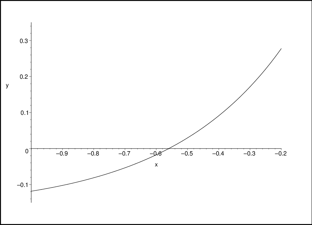
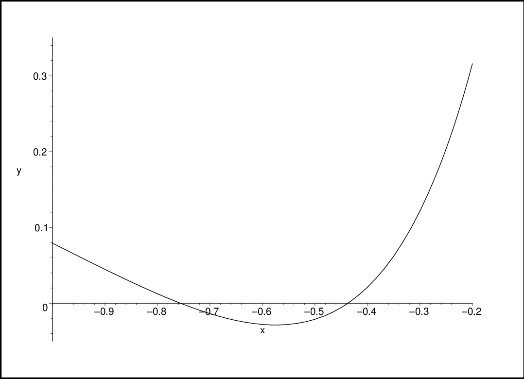
Figure 2 shows the functions $G_{\lambda}(z)$ (for the first six eigen-values) for real $z$ in the interval $[-1,-0.2]$. The choice of this interval is motivated by Theorem 5. Note also that functional equation implies $G_{\lambda}(0)=\big(\frac{1}{2}+\frac{1}{2\lambda}\big)G_{\lambda}(-1)$. Thus, one has $\frac{G_{\lambda}(0)}{G_{\lambda}(-1)}\rightarrow\infty$, as $\lambda\rightarrow 0$. This can also be seen empirically from Figure 2.
Summarizing, there are three objects associated with the Minkowski question mark function.

• •

  Distribution $F(x)$ = Functional equations (1) + Continuity.
  

• •

  Period function $G(z)$ = Three term functional equation (14) + Mild growth condition (as in Theorem 1).
  

• •

  Exponential generating function $m(t)$ = Integral equation (10) + boundary value and diminishing condition on the negative real line.
  

Each of them is characterized by the functional equation, and subject to some regularity conditions, it is unique, and thus arises exactly from $F(x)$. The objects are described via the “equality” Function = Equation + Condition. This means that the object on the left possesses both features; conversely - any object with these properties is necessarily the function on the left.
As expected, here we encounter the phenomena of “bootstrapping”: in all cases, regularity conditions can be significantly relaxed, and they are sufficient for the uniqueness, which automatically implies stronger regularity conditions. Here we show the rough picture of this phenomena. In each case, we suppose that the object satisfies the corresponding functional equation. For the details, see [2].

		$\displaystyle(i)$	$\displaystyle F(x)\text{ is continuous at one point }\Rightarrow F(x)\text{ is continuous}.$
		$\displaystyle(ii)$	$\displaystyle\text{ There exists }\varepsilon<1\text{ such that for every }z\text{ with }\Re z<0,\text{ we have }$
			$\displaystyle G(z-x)=O(2^{\varepsilon x})\text{ as }x\rightarrow\infty\Rightarrow G(z)=O(|z|^{-1})\text{ as }dist(z,\mathbb{R}_{+})\rightarrow\infty.$
		$\displaystyle(iii)$	$\displaystyle m^{\prime}(-t)=O(t^{-1})\text{ as }t\rightarrow\infty\Rightarrow|m(-t)|\ll e^{-\sqrt{t\log 2}}\text{ as }t\rightarrow\infty.$

Corresponding converse results were proved in [2]. For $F(x)$, this was in fact the starting point of these investigations, since the distribution of rationals in the Calkin-Wilf tree is a certain continuous function satisfying (1); thus, it is exactly $F(x)$. The converse result for $m(t)$ follows from Fredholm alternative, since all eigen-values of the operator (11) are strictly less than $1$ in absolute value. Finally, the converse theorem for $G(z)$ follows from a technical detail in the proof, which is the numerical estimate $0<\frac{\pi^{2}}{12}-\frac{\log^{2}2}{2}<1$; as a matter of fact, it appears that this is essentially the same argument as in the case of $m(t)$, since this constant gives the upper bound for the moduli of eigen-values.
One of the aims of this paper is to clarify the connections among these three objects, and to add the final fourth satellite, associated with $F(x)$. Henceforth, we have the complete list:

• •

  Zeta function $\,{\zeta_{\mathcal{M}}}(s)$ (see definition (26) below) = Functional equation with symmetry $s\rightarrow-s$ (27) + Regularity behavior in vertical strips.

In this case, we do not present a proof of a converse result. Indeed, the converse result for $G(z)$ is strongly motivated by its relation to Eisenstein series $G_{1}(z)$ (see [2] and the last Section). In the case of $\,{\zeta_{\mathcal{M}}}(s)$, this question is of small importance, and we rather concentrate on the direct result and its consequences.

In this section, we give another proof of (14), different from the one presented in [2], since it is considerably shorter. For our purposes, it is convenient to work in a slightly greater generality. Suppose that $\lambda\in\mathbb{R}$ has the property that there exists a function $F_{\lambda}(x)$, $x\in[0,\infty)$, such that

$\displaystyle\,{\rm{d}}F_{\lambda}(x+1)=\frac{1}{2}\,{\rm{d}}F_{\lambda}(x),\,{\rm{d}}F_{\lambda}\Big(\frac{1}{x}\Big)=\frac{1}{\lambda}\,{\rm{d}}F_{\lambda}(x).$

(16)

We omitted the word “continuous” in the description of the function intentionally. For a moment, consider $F_{\lambda}(x)=F(x)$ with $\lambda=-1$. Then $F_{-1}(x)$ is certainly continuous. The reason for introducing $\lambda$ will be apparent later. Thus, let

$\displaystyle G_{\lambda}(z)=\int\limits_{0}^{\infty}\frac{1}{x+1-z}\,{\rm{d}}F_{\lambda}(x).$

Since $F(x)+F(1/x)=1$, we see that for $\lambda=-1$ this agrees with the definition (12). This converges to an analytic function in the cut plane $\mathbb{C}\setminus(1,\infty)$. We have

	$\displaystyle 2G_{\lambda}(z+1)=2\int\limits_{0}^{1}\frac{1}{x-z}\,{\rm{d}}F_{\lambda}(x)+2\int\limits_{1}^{\infty}\frac{1}{x-z}\,{\rm{d}}F(x)=$
	$\displaystyle 2\int\limits_{0}^{\infty}\frac{1}{\frac{x}{x+1}-z}\,{\rm{d}}F_{\lambda}\Big(\frac{x}{x+1}\Big)+2\int\limits_{0}^{\infty}\frac{1}{x+1-z}\,{\rm{d}}F_{\lambda}(x+1)=$
	$\displaystyle\frac{2}{z}\int\limits_{0}^{\infty}\Big(\frac{x+1}{x+1-\frac{1}{z}}-1+1\Big)\,{\rm{d}}F_{\lambda}\Big(\frac{1}{x+1}\Big)+G_{\lambda}(z)=$
	$\displaystyle\frac{\alpha}{\lambda z}+\frac{1}{\lambda z^{2}}G_{\lambda}\Big(\frac{1}{z}\Big)+G_{\lambda}(z),\text{ where }\alpha=\int\limits_{0}^{\infty}\,{\rm{d}}F_{\lambda}(x).$

For $\lambda=-1$ and $F_{-1}(x)=F(x)$, this gives Theorem 1. Further, suppose $\lambda\neq-1$. Then

$\displaystyle\alpha=\int\limits_{0}^{\infty}\,{\rm{d}}F_{\lambda}(x)=\int\limits_{1}^{\infty}\,{\rm{d}}F_{\lambda}(x)+\int\limits_{0}^{1}\,{\rm{d}}F_{\lambda}(x)=\frac{\alpha}{2}-\frac{\alpha}{2\lambda}\Rightarrow\alpha=0.$

Therefore, the last functional equation reads as

$\displaystyle 2G_{\lambda}(z+1)=\frac{1}{\lambda z^{2}}G_{\lambda}\Big(\frac{1}{z}\Big)+G_{\lambda}(z).$

As a matter of fact, there cannot be any reasonable functions $F_{\lambda}(x)$, satisfying (16). Nevertheless, the last functional equation is identical to (15). Thus, Theorem 2 gives a description of all such possible $\lambda$. This suggests that we can still find certain distributions $F_{\lambda}(x)$. Further, as it was mentioned, $-1$ is not an-eigen value of (11). Due to the minus sign in front of the operator, this is exactly the exceptional eigen-value, which is essential in the Fredholm alternative. The above proof (rigid at least in case $\lambda=-1$), surprisingly, proves that the next tautological sentence has a certain point: “$-1$ is not an eigen-value because it is $-1$”. Indeed, we obtain non-homogeneous part of the three term functional equation only because $\lambda=-1$, since otherwise $\alpha=0$ and the equation is homogenic.
Distributions $F_{\lambda}(x)$ can indeed be strictly defined, at least in the space ${\sf C}^{\omega}$ of functions, which are analytic in the disk $\mathbf{D}=\{z:|z-\frac{1}{2}|\leq\frac{1}{2}\}$, including its boundary. This space is equipped with a topology of uniform convergence, and distribution on this space is any continuous linear functional. Indeed, since

$\displaystyle\int\limits_{0}^{1}\frac{x}{1-xz}\,{\rm{d}}F_{\lambda}(x)=-\frac{\lambda}{2}G_{\lambda}(z):=\sum\limits_{L=1}^{\infty}m^{(\lambda)}_{L}z^{L-1},$

define a distribution $F_{\lambda}$ on the space ${\sf C}^{\omega}$ by $\langle z^{L},F_{\lambda}\rangle=m^{\lambda}_{L}$, $L\geq 1$, $\langle 1,F_{\lambda}\rangle=0$, and for any analytic function $B(z)\in{\sf C}^{\omega}$, $B(z)=\sum_{L=0}^{\infty}b_{L}z^{L}$, by

$\displaystyle\langle B,F_{\lambda}\rangle=\sum\limits_{L=0}^{\infty}b_{L}\langle z^{L},F_{\lambda}\rangle.$

First, $\langle*,F_{\lambda}\rangle$ is certainly a linear functional and is properly defined, since the functional equation (15) for $G_{\lambda}(z)$ implies that it possesses all left derivatives at $z=1$; as a consequence, the series $\sum_{L=1}^{\infty}L^{p}|m^{(\lambda)}_{L}|$ converges for any $p\in\mathbb{N}$ (see Theorem 3 for the estimates on moments $m_{L}$). Second, let $B_{n}(z)=\sum_{L=0}^{\infty}b^{(n)}_{L}z^{L}$, $n\geq 1$, converge uniformly to $B(z)$ in the circle $|z|\leq 1$. Thus, $\sup_{|z|\leq 1}|B_{n}(z)-B(z)|=r_{n}\rightarrow 0$. Then by Cauchy formula,

$\displaystyle b^{(n)}_{L}=\frac{1}{2\pi i}\oint\limits_{|z|=1}\frac{B_{n}(z)}{z^{L+1}}\,{\rm{d}}z.$

This obviously imply that $|b^{(n)}_{L}-b_{L}|\leq r_{n}$, $L\geq 0$, and therefore $\langle*,F_{\lambda}\rangle$ is continuous, and hence it is a distribution. Using the condition $\,{\rm{d}}F_{\lambda}(x+1)=\frac{1}{2}\,{\rm{d}}F_{\lambda}(x)$, these distributions can be extended to other spaces. Summarizing, we have shown that Minkowski question mark function has an infinite sequence of “peers” $F_{\lambda}(x)$ which are also related to continued fraction expansion, in somewhat similar manner. $F(x)$ is the only one among them being “non-homogeneous”.

In this section we clarify the nature of linear relations among moments $M_{L}$. This was mentioned in [1], but not done in explicit form. Note that (9) gives linear relations among moments $m_{L}$: $m_{L}=\sum_{s=0}^{L}\binom{L}{s}(-1)^{s}m_{s}$, $L\geq 0$. These linear relations can be written in terms of $M_{L}$. Despite the fact that second equality of (9) is general phenomena for symmetric distribution, in conjunction with (8) it gives the essential information about $F(x)$. Therefore, let us denote

$\displaystyle{\sf q}(x,t)=(2-e^{t})e^{xt}-(2e^{t}-1)e^{-xt}=\sum\limits_{n=1}^{\infty}{\sf Q}_{n}(x)\frac{t^{n}}{n!}.$

We see that ${\sf Q}_{n}(x)$ are polynomials with integer coefficients and they are given by

$\displaystyle{\sf Q}_{n}(x)=2x^{n}-(x+1)^{n}-2(1-x)^{n}+(-x)^{n}.$

(17)

The following table gives the first few polynomials.

$n$	${\sf Q}_{n}(x)$	$n$	${\sf Q}_{n}(x)$
$1$	$2x-3$	$5$	$2x^{5}-15x^{4}+10x^{3}-30x^{2}+5x-3$
$2$	$2x-3$	$6$	$6x^{5}-45x^{4}+20x^{3}-45x^{2}+6x-3$
$3$	$2x^{3}-9x^{2}+3x-3$	$7$	$2x^{7}-21x^{6}+21x^{5}-105x^{4}+35x^{3}-63x^{2}+7x-3$
$4$	$4x^{3}-18x^{2}+4x-3$	$8$	$8x^{7}-84x^{6}+56x^{5}-210x^{4}+56x^{3}-84x^{2}+8x-3$

Moreover, the following statement holds.

Naturally, it is property $(iv)$ which makes these polynomials very important in the study of Minkowski’s $?(x)$. Here $L_{\mathbb{Q}}(*)$ denotes the $\mathbb{Q}-$linear space spanned by the specified polynomials.

Proof. (i) Let ${\sf q}_{e}(x,t)=\frac{1}{2}\big({\sf q}(x,t)+{\sf q}(x,-t)\big)$, and ${\sf q}_{o}(x,t)=\frac{1}{2}\big({\sf q}(x,t)-{\sf q}(x,-t)\big)$. Direct calculation shows that, if $e^{t}=T$, then

$\displaystyle 2{\sf q}_{e}=e^{xt}(3-T-\frac{2}{T})+e^{-xt}(3-\frac{1}{T}-2T),\quad 2{\sf q}_{o}=e^{xt}(1-T+\frac{2}{T})-e^{-xt}(1-\frac{1}{T}+2T).$

This yields

$\displaystyle\sum\limits_{n=1}^{\infty}{\sf Q}_{2n}(x)\frac{t^{2n}}{(2n)!}={\sf q}_{e}(x,t)=\frac{T-1}{T+1}{\sf q}_{o}(x,t)=\frac{e^{t}-1}{e^{t}+1}\sum\limits_{n=0}^{\infty}{\sf Q}_{2n+1}(x)\frac{t^{2n+1}}{(2n+1)!}.$

The multiplier on the right, $\frac{e^{t}-1}{e^{t}+1}=\tanh(t/2)$, is independent of $x$, and this obviously proves part $(i)$. Also, part (ii) follows easily from (17).
(iii) Since $\widehat{{\sf Q}}_{2n}(x)=\frac{1}{x}(3x^{2n}-(x+1)^{2n}-2(x-1)^{2n}+3)$, the proof is immediate.
(iv) In fact, (9) gives $(2-e^{t})M(t)=(2e^{t}-1)M(-t)$. For real $|t|<\log 2$, we have $M(t)=\int_{0}^{\infty}e^{xt}\,{\rm{d}}F(x)$. This implies

$\displaystyle\int\limits_{0}^{\infty}{\sf q}(x,t)\,{\rm{d}}F(x)=\sum\limits_{n=0}^{\infty}\frac{t^{n}}{n!}\int\limits_{0}^{\infty}{\sf Q}_{n}(x)\,{\rm{d}}F(x)\equiv 0,\quad\text{for }|t|<\log 2,$

and this completes the proof. $\blacksquare$
Consequently, there exist linear relations among moments $M_{L}$. Thus, for example, part $(iv)$ (in case $n=1$ and $n=3$) implies $2M_{1}-3=0$ and $2M_{3}-9M_{2}+3M_{1}=3$ respectively. The exact values of $M_{L}$ belong to the class of constants, which can be thought as emerging from arithmetic-geometric chaos. This resembles the situation concerning polynomial relations among various periods. We will not present the definition of a period, which can be found in [16]. In particular, the authors conjecture (and there is no support for possibility that it can be proved wrong) that “if a period has two integral representations, then one can pass from one formula to another using only additivity, change of variables, and Newton-Leibniz formula, in which all functions and domains of integration are algebraic with coefficients in $\overline{\mathbb{Q}}$”. Thus, for example, the conjecture predicts the possibility to prove directly that $\iint_{\frac{x^{2}}{4}+3y^{2}\leq 1}\,{\rm{d}}x\,{\rm{d}}y=\int_{-1}^{1}\frac{\,{\rm{d}}x}{\sqrt[3]{(1-x)(1+x)^{2}}},$ without knowing that they both are equal to $\frac{2\pi}{\sqrt{3}}$, and this indeed can be done. Similarly, returning to the topic of this paper, we believe that any finite $\mathbb{Q}-$linear relation among constants $M_{L}$ can be proved simply by applying the functional equation of $F(x)$, by means of integration by parts and change of variables. The last proposition supports this claim. In other words, we believe that there cannot be any other miraculous coincidences regarding the values of $M_{L}$. More precisely,

Conjecture. Suppose, $r_{k}\in\mathbb{Q}$, $0\leq k\leq L$, are rational numbers such that $\sum_{k=0}^{L}r_{k}M_{k}=0$. Let $\ell=\big[\frac{L-1}{2}\big]$. Then

$\displaystyle\sum\limits_{k=0}^{L}r_{k}x^{k}\in L_{\mathbb{Q}}\big({\sf Q}_{1}(x),{\sf Q}_{3}(x),...,{\sf Q}_{2\ell+1}(x)\big).$

This conjecture, if true, should be difficult to prove. It would imply, for example, that $M_{L}$ for $L\geq 2$ are irrational. On the other hand, this conjecture seems to be much more natural and approachable, compared to similar conjectures regarding arithmetic nature of constants emerging from geometric chaos, e.g. spectral values $s$ for Maass wave forms (say, for ${\sf PSL}_{2}(\mathbb{Z})$), or those coming from arithmetic chaos, like non-trivial zeros of Riemann’s $\zeta(s)$. We cannot give any other evidence, save the last proposition, to support this conjecture.