1The Reissner–Nordström black hole

28 December 2007

Ruppeiner Geometry of Black Hole Thermodynamics

Jan E. Åman¹¹ 1 ja@physto.se, Narit Pidokrajt²² 2 narit@physto.se

Department of Physics
Stockholm University
SE-106 91 Stockholm
Sweden

We are here not studying the spacetimes of black holes as such. Instead we examine entropy $S(M,Q,J)$ or mass $M(S,Q,J)$ , where $Q$ is charge and $J$ angular momentum. The Ruppeiner metric [1] is the Hessian of negative entropy: $g^{R}_{ij}=-\partial_{i}\partial_{j}S(M,N^{a})$ while the Weinhold metric [2] is the Hessian of $M$ : $g^{W}_{ij}=\partial_{i}\partial_{j}M(S,N^{a})$ . The two metrics are conformally related $ds^{2}=g^{R}_{ij}dM^{i}dM^{j}=\frac{1}{T}g^{W}_{ij}dS^{i}dS^{j}$ where $M^{i}=(M,N^{a})$ , $S^{i}=(S,N^{a})$ and $T=\frac{\partial M}{\partial S}$ is the temperature.

Abstract

The Hessian of the entropy function can be thought of as a metric tensor on state space. In the context of thermodynamical fluctuation theory Ruppeiner has argued that the Riemannian geometry of this metric gives insight into the underlying statistical mechanical system; the claim is supported by numerous examples. We study these geometries for some families of black holes and find that the Ruppeiner geometry is flat for Reissner–Nordström black holes in any dimension, while curvature singularities occur for the Kerr black holes. Kerr black holes have instead flat Weinhold curvature.

1 The Reissner–Nordström black hole

The event horizon is given by

||{\xi}||^{2}=-\left(1-\frac{2M}{r}+\frac{Q^{2}}{r^{2}}\right)=0\ ,

(1)

where $r$ is chosen so that the area of a sphere at constant $r$ equals $4{\pi}r^{2}$ . There are two roots $r_{+}$ and $r_{-}$ . We find that $M=\frac{1}{2}(r_{+}+r_{-})$ , $Q^{2}=r_{+}r_{-}\$ , $r_{+}=\!M+\sqrt{M^{2}-Q^{2}}=\!M\,\left(1+\sqrt{1-\frac{Q^{2}}{M^{2}}}\right)$ . The entropy is $S=\frac{k}{4}A=k{\pi}r_{+}^{\,\,2}=r_{+}^{\,\,2}\$ , and we set $k=1/{\pi}$ . Solving for $M$ the fundamental thermodynamical relation is $M=\frac{\sqrt{S}}{2}\left(1+\frac{Q^{2}}{S}\right)$ . The temperature is $T=\frac{\partial M}{\partial S}=\frac{1}{4\sqrt{S}}\left(1-\frac{Q^{2}}{S}\right)$ . In its natural coordinates the Weinhold metric becomes [3]

ds^{2}_{W}=\frac{1}{8S^{\frac{3}{2}}}\bigg(-\left(1-\frac{3Q^{2}}{S}\right)dS^{2}-8QdQdS+8SdQ^{2}\bigg)\ .

(2)

Introducing new coordinate $u=\frac{Q}{\sqrt{S}}$ ; $-1\leq u\leq 1$ we now find that

ds^{2}_{W}=\frac{1}{8S^{\frac{3}{2}}}\left(-(1-u^{2})dS^{2}+8S^{2}du^{2}\right)\ .

(3)

In these coordinates the Ruppeiner metric is given by

ds^{2}_{R}=\frac{1}{T}ds^{2}_{W}=-\frac{dS^{2}}{2S}+\frac{4Sdu^{2}}{1-u^{2}}\ .

(4)

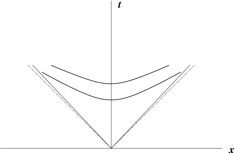
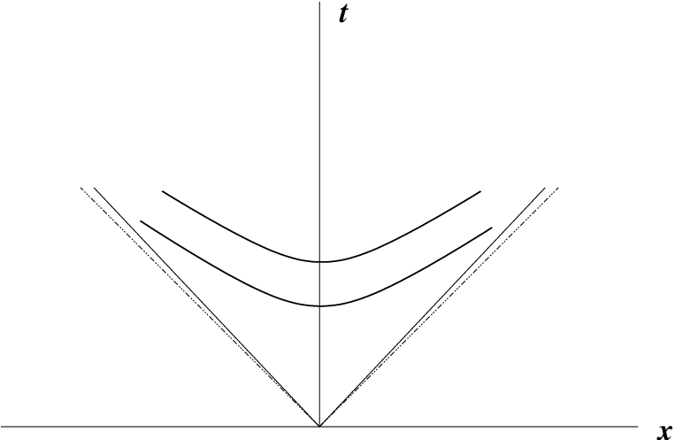
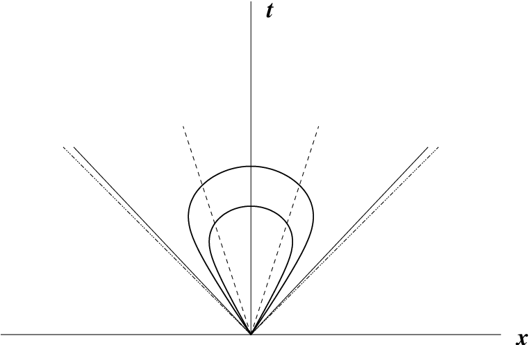
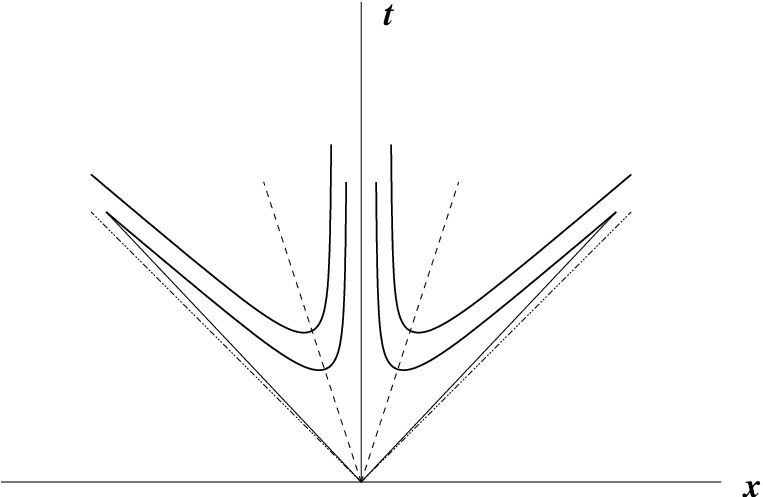
This metric is flat! To see this introduce new coordinates ${\tau}=\sqrt{2S}$ , $\sin{\frac{\chi}{\sqrt{2}}}=u$ . The Ruppeiner metric now takes Rindler form $ds^{2}_{R}=-d{\tau}^{2}+{\tau}^{2}d{\chi}^{2}$ , $\tau$ and $\chi$ are Rindler coordinates on the forward light cone in Minkowski space. In Fig. 1 we use the inertial coordinates $t=\tau\cosh{\chi}$ , $x=\tau\sinh{\chi}$ .

Refer to caption — Figure 1: The state space of the Reissner-Nordström black hole is a wedge inside the forwards light cone of a 1+1 dimensional Minkowski space. We show curves of constant entropy (spacelike hyperbolas), constant mass (also spacelike), constant temperature, and constant charge. The latter two become null at the “Davies point”, $Q/M=\sqrt{3}/2$ [4] which is given by a dashed line of constant electric potential.

2 Kerr black hole, spacetime dimension ${\bf\it d}$

In higher dimensional spacetimes there can be more than one angular momentum. For the Kerr black hole with a single nonzero spin we obtain the event horizon from [5]

r_{+}^{\,\,2}+a^{2}-\frac{\mu}{r_{+}^{\,\,d-5}}=0.

(5)

The area of the event horizon is given by $A=\Omega_{(d-2)}r_{+}^{\,\,d-4}\>(r_{+}^{\,\,2}+a^{2})$ where $\Omega_{d}$ is the area of the unit $d$ -sphere. The ADM mass of the hole is defined by $\mu=\frac{4M}{d-2}$ . The angular momentum per unit mass is $a=\frac{d-2}{2}\frac{J}{M}$ . We have $S=\frac{kA}{4G}$ and set $\displaystyle k=1/\pi$ and set Newton’s constant $G$ to $\Omega_{(d-2)}/4\pi$ to obtain the entropy $S=r_{+}^{\,\,d-4}(r_{+}^{\,\,2}+a^{2})=r_{+}\mu.$ Explicit $S$ in arbitrary dimension cannot be obtained, but we can work via the Weinhold metric. The mass is

M=\frac{d-2}{4}S^{\frac{d-3}{d-2}}\left(1+\frac{4J^{2}}{S^{2}}\right)^{1/(d-2)}.

(6)

The Weinhold metric $g^{W}_{ij}=\partial_{i}\partial_{j}M(S,J)$ of the $d$ -dimensional Kerr black hole is found to be flat! In a diagonal form [6]:

ds^{2}_{W}=-d\tau^{2}+{\frac{2(d-3)}{(d-2)}}{\frac{(1-4{\frac{d-5}{d-3}}u^{2})}{(1+4u^{2})^{2}}}\tau^{2}du^{2}.

(7)

$u=\frac{1}{2}\sinh 2\sigma$ gives Rindler coordinates for $d=4$ : $ds^{2}_{W}=-d\tau^{2}+\tau^{2}d\sigma^{2}$ . For $d=4$ the extremal limit is $J/M^{2}=1$ , hence $u$ is bounded by $\left|u\right|\leq\frac{1}{2}\Leftrightarrow\left|\sigma\right|\leq\frac{1}{2}\sinh^{-1}1\approx 0.4406$ . In Minkowski style coordinates the state space of the Kerr black hole is a wedge bounded by $\left|\frac{x}{t}\right|\leq\sqrt{\frac{\sqrt{2}-1}{\sqrt{2}+1}}$ . For $d=5$ the extremal limit is given by $J^{2}/M^{3}=16/27$ and $-\infty\leq u\leq\infty$ where $u=\frac{1}{2}\tan\sqrt{3}\sigma$ . Hence we obtain a wedge with wider opening angle $\left|\sigma\right|\leq\frac{1}{\sqrt{3}}\arctan\infty=\frac{\pi}{2\sqrt{3}}\approx 0.9069$ .

Remarkably, the wedge of the $d\geq 6$ Kerr black hole fills the entire light cone. This is because for black holes in $d\geq 6$ there are no extremal limits.

In any dimension, we obtain the Ruppeiner metric from the Weinhold metric using the conformal relation. It is a curved metric with the curvature scalar

\displaystyle\mathcal{R}=-\frac{1}{S}\frac{\displaystyle 1-12\frac{d-5}{d-3}\frac{J^{2}}{S^{2}}}{\displaystyle\left(1-4\frac{d-5}{d-3}\frac{J^{2}}{S^{2}}\right)\left(1+4\frac{d-5}{d-3}\frac{J^{2}}{S^{2}}\right)}.

(8)

In $d=4$ the curvature scalar diverges along the curve $4J^{2}=S^{2}$ . In $d=5$ the curvature is reduced to $\mathcal{R}=-\frac{1}{S}$ which diverges in the extremal limit of the $d=5$ Kerr black hole.

For $d\geq 6$ we have a curvature blow-up but not in the limit of extremal black hole, rather at $4J^{2}=\frac{d-3}{d-5}S^{2}$ . This is where Emparan and Myers [7] suggest that the Kerr black hole becomes unstable and changes its behavior to be like a black membrane.

Note that in $d=5$ for some values of the parameters, there exist “black ring” solutions [8] whose entropy is larger than that of the black hole studied in our papers. A careful observation of curvature scalar $\mathcal{R}=-\frac{1}{S}$ indicates that nothing special happens to the Gibbs surface of the Kerr black hole a la Myers-Perry.

3 Our flatness theorem

We can now state a small theorem, namely: If $\psi(x,y)=x^{a}f(y/x)$ then the information metric is flat [9]. The converse does not hold. The most straightforward way to prove the theorem is to change to the new coordinates $\psi=x^{a}f(x^{b}y)$ , and $\sigma=x^{b}y$ . An explicit calculation shows that

	$\displaystyle ds^{2}$	$\displaystyle=$	$\displaystyle\left(\frac{a-1}{a}-\frac{b(b+1)}{a^{2}}\frac{\sigma f^{\prime}}{f}\right)\frac{d\psi^{2}}{\psi}+2(b+1)\left(\frac{1}{a}\frac{f^{\prime}}{f}\frac{b}{a^{2}}+\frac{\sigma f^{\prime 2}}{f^{2}}\right)d\psi d\sigma$		(9)
		$\displaystyle+$	$\displaystyle\psi\left(\frac{f^{\prime\prime}}{f}-\frac{2b+a+1}{a}\frac{f^{\prime 2}}{f^{2}}-\frac{b(b+1)}{a^{2}}\frac{\sigma f^{\prime 3}}{f^{3}}\right)d\sigma^{2}\ .$		(9)

This is diagonal if $b=-1$ . If we introduce the new coordinate $r=\sqrt{\psi}$ it is also manifestly a flat metric, and it covers a wedge shaped region. Given the function $f$ we can reparametrize $\sigma$ so that we end up with polar coordinates, or Rindler coordinates if the metric is Lorentzian, and read off the opening angle of the wedge. Anyway the small theorem is proved. There is an exception if $b=-1$ and $a=1$ , since then the metric is degenerate.

We can restate our small theorem in thermodynamical language: Let $S=M^{a}f(M^{b}Q)$ . If $b=-1$ the Ruppeiner metric is flat. If $a+b=0$ the Weinhold metric is flat.

An explicit example: The Reissner–Nordström black hole in arbitrary spacetime dimension $d$ has the fundamental relation $S=M^{c}\left(1+\sqrt{1-\frac{c}{2}\frac{Q^{2}}{M^{2}}}\right)^{c}$ , $c\equiv\frac{d-2}{d-3}$ . The Ruppeiner geometry is a timelike wedge in a flat Minkowski space, with an opening angle that grows with $d$ . It is a black hole if $d\geq 4$ .

This theorem is now helping us treating other sorts of black holes as e.g. dilaton black holes, see [10, 11] and forthcoming papers.

For computer algebra calculations we used GRTENSOR for MAPLE and CLASSI.

Several interesting papers has recently been published, see for instance Arcioni & Lozano-Tellechea [12], Shen et al. [13], Quevedo [14], Mirza & Zamani-Nasab [15] and Ruppeiner [16].

4 Summary of results

Spacetime dimension	Black hole family	Ruppeiner	Weinhold
any $d\geq 4$	Kerr	Curved	Flat
	Reissner–Nordström	Flat	Curved
$d=4$	Kerr-Newman	Curved	Curved
	RN-anti-de Sitter	Curved	Curved
$d=5$	double-spin Kerr	Curved	Curved

Table 1: Geometry of black hole thermodynamics.

Acknowledgments

We thank Ingemar Bengtsson for valuable discussions.

References

[1] Ruppeiner, G. 1995, Rev. Mod. Phys., 67, 605.
[2] Weinhold, F. 1975, Chem. Phys., 63, 2479.
[3] Åman, J.E., Bengtsson, I. & Pidokrajt, N. 2003, Gen. Rel. Grav., 35, 1733.
[4] Davies, P.C.W. 1977, Proc. Roy. Soc., A353, 499.
[5] Myers, P.C. & Perry, M.J. 1986, Ann. Phys., 172, 304.
[6] Åman, J.E. & Pidokrajt, N. 2006, Phys. Rev. D., 73, 024017.
[7] Emparan, R. & Myers, R.C. 2003, JHEP 09, 025.
[8] Emparan, R. & Reall, H.S. 2002, Phys. Rev. Lett., 88, 101101.
[9] Åman, J.E., Bengtsson, I. & Pidokrajt, N. 2006, Gen. Rel. Grav., 38, 1305.
[10] Åman, J.E., Bedford, J., Grumiller, D., Pidokrajt, N. & Ward, J. 2007, J. Phys.: Conf. Ser., 66, 012007.
[11] Åman, J.E., Pidokrajt, N. & Ward, J. 2007, arXiv:0711.2201.
[12] Arcioni, G. & Lozano-Tellechea, E. 2005, Phys. Rev. D., 72, 104021.
[13] Shen, J., Cai, R-G., Wang, B. & Su, R-K. 2006, Int. J. Mod. Phys., A22, 11-27.
[14] Quevedo, H. 2007, arXiv:0704.3102.
[15] Mirza, B. & Zamani-Nasab, M. 2007, JHEP, 06, 059.
[16] Ruppeiner, G. 2007, arXiv:0711.4328.


Entropy	Mass

Temperature	Charge