跳到论文正文
W Papers独立论文阅读器 arXiv:0712.4400 论文正文 计算阅读时间 · 0%
引用这篇论文根据当前论文元数据生成,正式投稿前建议核对。


License: Assumed arXiv.org perpetual non-exclusive license
arXiv:0712.4400v1 [math.OC] 28 Dec 2007

Geometric structure-preserving optimal control of the rigid body

Anthony M. Bloch Address: Alexander Ziwet Collegiate Professor of Mathematics and Department Chair, Mathematics, University of Michigan Email address: abloch@umich.edu , Islam I. Hussein Address: Assistant Professor, Mechanical Engineering, Worcester Polytechnic Institute Email address: ihussein@wpi.edu , Melvin Leok Address: Assistant Professor, Mathematics, Purdue University Email address: mleok@math.purdue.edu and Amit K. Sanyal Address: Assistant Professor, Mechanical Engineering, University of Hawaii Email address: aksanyal@hawaii.edu
Date: Received: date / Revised: date
Abstract.

In this paper we study a discrete variational optimal control problem for the rigid body. The cost to be minimized is the external torque applied to move the rigid body from an initial condition to a pre-specified terminal condition. Instead of discretizing the equations of motion, we use the discrete equations obtained from the discrete Lagrange–d’Alembert principle, a process that better approximates the equations of motion. Within the discrete-time setting, these two approaches are not equivalent in general. The kinematics are discretized using a natural Lie-algebraic formulation that guarantees that the flow remains on the Lie group SO​(3)\textsf{SO}(3) and its algebra 𝔰​𝔬​(3)\mathfrak{so}(3). We use Lagrange’s method for constrained problems in the calculus of variations to derive the discrete-time necessary conditions. We give a numerical example for a three-dimensional rigid body maneuver.

1. Introduction

This paper deals with a structure-preserving computational approach to the optimal control problem of minimizing the control effort necessary to perform an attitude transfer from an initial state to a prescribed final state, in the absence of a potential field. The configuration of the rigid body is given by the rotation matrix from the body frame to the spatial frame, which is an element of the group of orientation-preserving isometries in ℝ3\mathbb{R}^{3}. The state of the rigid body is described by the rotation matrix and its angular velocity.

To motivate the computational approach we adopt in the discrete-time case, we first revisit the variational continuous-time optimal control problem. The continuous-time extremal solutions to this optimal control problem have certain special features, since they arise from variational principles. General numerical integration methods, including the popular Runge-Kutta schemes, typically preserve neither first integrals nor the characteristics of the configuration space. Geometric integrators are the class of numerical integration schemes that preserve such properties, and a good survey can be found in [5]. Techniques particular to Hamiltonian systems are also discussed in [16] and [24].

Our approach to discretizing the optimal control problem is in contrast to traditional techniques such as collocation, wherein the continuous equations of motion are imposed as constraints at a set of collocation points. In our approach, modeled after [11], the discrete equations of motion are derived from a discrete variational principle, and this induces constraints on the configuration at each discrete time step.

This approach yields discrete dynamics that are more faithful to the continuous equations of motion, and consequently yields more accurate solutions to the optimal control problem that is being approximated. This feature is extremely important in computing accurate (sub)optimal trajectories for long-term spacecraft attitude maneuvers. For example, in [9], the authors propose an imaging spacecraft formation design that requires a continuous attitude maneuver over a period of 77 days in a low Earth orbit. Hence, attitude maneuver has to be very accurate to meet tight imaging constraints over long time ranges.

While the discrete optimal control method presented here is illustrated using the Lie group SO​(3)\textsf{SO}(3) of rotation matrices, and its corresponding Lie algebra 𝔰​𝔬​(3)\mathfrak{so}(3) of skew-symmetric matrices, we have derived the method with sufficient generality to address the problem of optimal control on arbitrary Lie groups with the drift vector field given by geodesic flow on the group, and it therefore widely applicable. For example, in inter-planetary orbit transfers (see, for example, [1]), one is interested in computing optimal or suboptimal trajectories on the group of rigid body motions SE​(3)\textsf{SE}(3) with a high degree of accuracy. Similar requirements also apply to the control of quantum systems. For example, efficient construction of quantum gates is a problem on the unitary Lie group SU​(N)\textsf{SU}(N). This is an optimal control problem, where one wishes to steer the identity operator to the desired unitary operator (see, for example, [13] and [23]).

Moreover, an important feature of the way we discretize the optimal control problem is that it is SO​(3)\textsf{SO}(3)-equivariant. The SO​(3)\textsf{SO}(3)-equivariance of our numerical method is desirable, since it ensures that our results do not depend on the choice of coordinates and coordinate frames. This is in contrast to methods based on coordinatizing the rotation group using quaternions, (modified) Rodrigues parameters, and Euler angles, as given in the survey [26]. Even if the optimal cost function is SO​(3)\textsf{SO}(3)-invariant, as in [25], the use of generalized coordinates imposes constraints on the attitude kinematics.

For the purpose of numerical simulation, the corresponding discrete optimal control problem is posed on the discrete state space as a two stage discrete variational problem. In the first step, we derive the discrete dynamics for the rigid body in the context of discrete variational mechanics [20]. This is achieved by considering the discrete Lagrange–d’Alembert variational principle [12] in combination with essential ideas from Lie group methods [10], which yields a Lie group variational integrator [17]. This integrator explicitly preserves the Lie group structure of the configuration space, and is similar to the integrators introduced in [14] for a rigid body in an external field, and in [15] for full body dynamics. These discrete equations are then imposed as constraints to be satisfied by the extremal solutions to the discrete optimal control problem, and we obtain the discrete extremal solutions in terms of the given terminal states.

The paper is organized as follows. As motivation, in Section 2, we study the minimum control effort optimal control problem in continuous-time. In Section 3, we study the corresponding discrete-time optimal control problem. In Section 3.1 we state the optimal control problem and describe our approach. In Section 3.2, we derive the discrete-time equations of motion for the rigid body starting with the discrete Lagrange–d’Alembert principle. These equations are used in Section 3.3 to obtain the solution to the discrete optimal control problem. In Section 5, we describe an algorithm for solving the general nonlinear, implicit necessary conditions for SO​(3)\textsf{SO}(3) and give numerical examples for rest-to-rest and slew-up spacecraft maneuvers.

2. Continuous-Time Results

2.1. Problem Formulation

In this paper, the natural pairing between 𝔰​𝔬∗​(3)\mathfrak{so}^{*}(3) and 𝔰​𝔬​(3)\mathfrak{so}(3) is denoted by ⟨⋅,⋅⟩\left<\cdot,\cdot\right>. Let ≪⋅,⋅≫\ll\cdot,\cdot\gg and ≪⋅,⋅≫∗\ll\cdot,\cdot\gg_{*} denote the standard (induced by the Killing form) inner product on 𝔰​𝔬​(3)\mathfrak{so}(3) and 𝔰​𝔬∗​(3)\mathfrak{so}^{*}(3), respectively. The inner product ≪⋅,⋅≫∗\ll\cdot,\cdot\gg_{*} is naturally induced from the standard norm ≪𝝃,𝝎≫=−12Tr(𝝃T𝝎)\ll\boldsymbol{\xi},\boldsymbol{\omega}\gg=-\frac{1}{2}{\rm Tr}(\boldsymbol{\xi}^{T}\boldsymbol{\omega}), for all 𝝃,𝝎∈𝔰​𝔬​(3)\boldsymbol{\xi},\boldsymbol{\omega}\in\mathfrak{so}(3), through

(1) ≪𝜼,𝝋≫∗\displaystyle\ll\boldsymbol{\eta},\boldsymbol{\varphi}\gg_{*} =\displaystyle= ⟨𝜼,𝝋♯⟩=⟨𝜼,𝝎⟩=⟨𝝃♭,𝝎⟩\displaystyle\left<\boldsymbol{\eta},\boldsymbol{\varphi}^{\sharp}\right>=\left<\boldsymbol{\eta},\boldsymbol{\omega}\right>=\left<\boldsymbol{\xi}^{\flat},\boldsymbol{\omega}\right>
=\displaystyle= ≪𝝃,𝝎≫,\displaystyle\ll\boldsymbol{\xi},\boldsymbol{\omega}\gg,

where 𝝋=𝝎♭∈𝔰​𝔬∗​(3)\boldsymbol{\varphi}=\boldsymbol{\omega}^{\flat}\in\mathfrak{so}^{*}(3) and 𝜼=𝝃♭∈𝔰​𝔬∗​(3)\boldsymbol{\eta}=\boldsymbol{\xi}^{\flat}\in\mathfrak{so}^{*}(3), with 𝝃,𝝎∈𝔰​𝔬​(3)\boldsymbol{\xi},\boldsymbol{\omega}\in\mathfrak{so}(3) and ♭\flat and ♯\sharp are the musical isomorphisms with respect to the standard metric ≪⋅,⋅≫\ll\cdot,\cdot\gg. On 𝔰​𝔬​(3)\mathfrak{so}(3), these isomorphisms correspond to the transpose operation. That is, we have 𝝋=𝝎T\boldsymbol{\varphi}=\boldsymbol{\omega}^{\textrm{T}} and 𝜼=𝝃T\boldsymbol{\eta}=\boldsymbol{\xi}^{\textrm{T}}.

Let 𝐉:𝔰​𝔬​(3)→𝔰​𝔬∗​(3)\mathbf{J}:\mathfrak{so}(3)\rightarrow\mathfrak{so}^{*}(3) be the positive definite inertia operator. It can be shown that

(2) ⟨𝐉⁡(𝝃),𝝎⟩=⟨𝐉⁡(𝝎),𝝃⟩.\displaystyle\left<\mathbf{J}(\boldsymbol{\xi}),\boldsymbol{\omega}\right>=\left<\mathbf{J}(\boldsymbol{\omega}),\boldsymbol{\xi}\right>.

On 𝔰​𝔬​(3)\mathfrak{so}(3), 𝐉\mathbf{J} is given by 𝐉⁡(𝝃)=J​𝝃+𝝃​J\mathbf{J}(\boldsymbol{\xi})=J\boldsymbol{\xi}+\boldsymbol{\xi}J, where JJ is a positive definite symmetric matrix (see, for example, [3, 8]). Moreover, we also have 𝐉​(𝜼♯)♯=(J​𝜼T+𝜼T​J)T=𝐉⁡(𝜼)\mathbf{J}(\boldsymbol{\eta}^{\sharp})^{\sharp}=(J\boldsymbol{\eta}^{\textrm{T}}+\boldsymbol{\eta}^{\textrm{T}}J)^{\textrm{T}}=\mathbf{J}(\boldsymbol{\eta}), which is an abuse of notation since 𝜼∈𝔰​𝔬∗​(3)\boldsymbol{\eta}\in\mathfrak{so}^{*}(3). For the sake of generality and mathematical precision we will use the general definitions, though it helps to keep the above identifications for 𝔰​𝔬​(3)\mathfrak{so}(3) in mind.

In this section we review some continuous-time optimal control results using a simple optimal control example on SO​(3)\textsf{SO}(3). The problem we consider is that of minimizing the norm squared of the control torque 𝝉∈𝔰​𝔬∗​(3)\boldsymbol{\tau}\in\mathfrak{so}^{*}(3) applied to rotate a rigid body subject to the Lagrange--d’Alembert principle for the rigid body11 1 This is equivalent to constraining the problem to satisfy the rigid body equations of motion given by equations (7). However, for the sake of generality that will be appreciated in the discrete-time problem, we choose to treat the Lagrange–d’Alembert principle as the constraint as opposed to the rigid body equations of motion. Both are equivalent in the continuous-time case but are generally not equivalent in the discrete-time case. whose configuration is given by 𝐑∈SO​(3)\mathbf{R}\in\textsf{SO}(3) and body angular velocity is given by 𝛀∈𝔰​𝔬​(3)\mathbf{\Omega}\in\mathfrak{so}(3). We require that the system evolve from an initial state (𝐑0,𝛀0)(\mathbf{R}_{0},\mathbf{\Omega}_{0}) to a final state (𝐑T,𝛀T)(\mathbf{R}_{T},\mathbf{\Omega}_{T}) at a fixed terminal time TT.

Before proceeding with a statement of the optimal control problem, we first define variations of the rigid body configuration 𝐑\mathbf{R} and its velocity 𝛀\mathbf{\Omega}. Let 𝐖⁡(t)∈𝔰​𝔬​(3)\mathbf{W}(t)\in\mathfrak{so}(3) be the variation vector field associated with a curve 𝐑⁡(t)\mathbf{R}(t) on SO​(3)\textsf{SO}(3) [2, 28]. The vector field 𝐖⁡(t)\mathbf{W}(t) satisfies

𝜹​𝐑​(t)=𝐑𝐖∈T𝐑⁡(t)​SO​(3),𝐖⁡(0)=𝟎,𝐖⁡(T)=𝟎,\displaystyle\boldsymbol{\delta}\mathbf{R}(t)=\mathbf{R}\mathbf{W}\in\textsf{T}_{\mathbf{R}(t)}\textsf{SO}(3),~\mathbf{W}(0)=\mathbf{0},~\mathbf{W}(T)=\mathbf{0},

where 𝜹​𝐑\boldsymbol{\delta}\mathbf{R} is defined by 𝜹​𝐑​(t)=∂𝐑ϵ​(t)/∂ϵ|ϵ=0\boldsymbol{\delta}\mathbf{R}(t)=\partial\mathbf{R}_{\epsilon}(t)/\partial\epsilon\big|_{\epsilon=0}, with 𝐑ϵ​(t):=𝐑⁡(t,ϵ)\mathbf{R}_{\epsilon}(t):=\mathbf{R}(t,\epsilon) is the variation of the curve 𝐑⁡(t)\mathbf{R}(t) that satisfies 𝐑⁡(t,0)=𝐑⁡(t)\mathbf{R}(t,0)=\mathbf{R}(t). The variation in the velocity vector field is denoted 𝜹​𝛀\boldsymbol{\delta}\mathbf{\Omega}. For a deeper understanding of variations of general vector fields, see for example the treatment in [7].

We now state the minimum control effort optimal control problem.

Problem 2.1.

Minimize

(3) 𝒥\displaystyle\mathcal{J} =\displaystyle= 12∫0T≪𝝉,𝝉≫∗dt\displaystyle\frac{1}{2}\int_{0}^{T}\ll\boldsymbol{\tau},\boldsymbol{\tau}\gg_{*}{\rm d}t

subject to

  1. (1)

    satisfying Lagrange–d’Alembert principle:

    (4) 𝜹​∫0T12​⟨𝐉⁡(𝛀),𝛀⟩​𝑑t+∫0T⟨𝝉,𝐖⟩​𝑑t=0,\displaystyle\boldsymbol{\delta}\int_{0}^{T}\frac{1}{2}\left<\mathbf{J}\left(\mathbf{\Omega}\right),\mathbf{\Omega}\right>{\rm d}t+\int_{0}^{T}\left<\boldsymbol{\tau},\mathbf{W}\right>{\rm d}t=0,

    for a variation vector field 𝐖⁡(t)\mathbf{W}(t), and subject to 𝐑˙=𝐑​𝛀\dot{\mathbf{R}}=\mathbf{R}\mathbf{\Omega},

  2. (2)

    and the boundary conditions

    𝐑⁡(0)\displaystyle\mathbf{R}(0) =\displaystyle= 𝐑0,𝛀⁡(0)=𝛀0,\displaystyle\mathbf{R}_{0},~\mathbf{\Omega}(0)=\mathbf{\Omega}_{0},
    (5) 𝐑⁡(T)\displaystyle\mathbf{R}(T) =\displaystyle= 𝐑T,𝛀⁡(T)=𝛀T.\displaystyle\mathbf{R}_{T},~\mathbf{\Omega}(T)=\mathbf{\Omega}_{T}.

We now show that the constraint of satisfying the Lagrange–d’Alembert principle leads to the following problem formulation, where the rigid body equations of motion replace the Lagrange–d’Alembert principle.

Problem 2.2.

Minimize

(6) 𝒥\displaystyle\mathcal{J} =\displaystyle= 12∫0T≪𝝉,𝝉≫∗dt\displaystyle\frac{1}{2}\int_{0}^{T}\ll\boldsymbol{\tau},\boldsymbol{\tau}\gg_{*}{\rm d}t

subject to

  1. (1)

    the dynamics

    (7) 𝐑˙\displaystyle\dot{\mathbf{R}} =\displaystyle= 𝐑​𝛀\displaystyle\mathbf{R}\mathbf{\Omega}
    𝐌˙\displaystyle\dot{\mathbf{M}} =\displaystyle= ad𝛀∗​𝐌+𝝉=[𝐌,𝛀]+𝝉,\displaystyle{\rm ad}_{\mathbf{\Omega}}^{*}\mathbf{M}+\boldsymbol{\tau}=\left[\mathbf{M},\mathbf{\Omega}\right]+\boldsymbol{\tau},

    where 𝐌=𝐉⁡(𝛀)∈𝔰​𝔬∗​(3)\mathbf{M}=\mathbf{J}(\mathbf{\Omega})\in\mathfrak{so}^{*}(3) is the momentum,

  2. (2)

    and the boundary conditions

    𝐑⁡(0)\displaystyle\mathbf{R}(0) =\displaystyle= 𝐑0,𝛀⁡(0)=𝛀0,\displaystyle\mathbf{R}_{0},~\mathbf{\Omega}(0)=\mathbf{\Omega}_{0},
    (8) 𝐑⁡(T)\displaystyle\mathbf{R}(T) =\displaystyle= 𝐑T,𝛀⁡(T)=𝛀T.\displaystyle\mathbf{R}_{T},~\mathbf{\Omega}(T)=\mathbf{\Omega}_{T}.

In the above, ad∗{\rm ad}^{*} is the dual of the adjoint representation, ad{\rm ad}, of 𝔰​𝔬​(3)\mathfrak{so}(3) and is given by ad𝝃∗​𝜼=−[𝝃,𝜼]∈𝔰​𝔬∗​(3){\rm ad}_{\boldsymbol{\xi}}^{*}\boldsymbol{\eta}=-[\boldsymbol{\xi},\boldsymbol{\eta}]\in\mathfrak{so}^{*}(3), for all 𝝃∈𝔰​𝔬​(3)\boldsymbol{\xi}\in\mathfrak{so}(3) and 𝜼∈𝔰​𝔬∗​(3)\boldsymbol{\eta}\in\mathfrak{so}^{*}(3). Recall that the bracket is defined by [𝝃,𝝎]=𝝃​𝝎−𝝎​𝝃\left[\boldsymbol{\xi},\boldsymbol{\omega}\right]=\boldsymbol{\xi}\boldsymbol{\omega}-\boldsymbol{\omega}\boldsymbol{\xi}.

2.2. The Lagrange–d’Alembert Principle and the Rigid Body Equations of Motion

In this section we derive the forced rigid body equations of motion (equations (7)) from the Lagrange–d’Alembert principle. We begin by appending the constraint 𝐑˙=𝐑​𝛀\dot{\mathbf{R}}=\mathbf{R}\mathbf{\Omega} to the Lagrangian

0\displaystyle 0 =\displaystyle= 𝜹​∫0T(12​⟨𝐉⁡(𝛀),𝛀⟩+⟨𝚲,𝐑−1​𝐑˙−𝛀⟩)​𝑑t\displaystyle\boldsymbol{\delta}\int_{0}^{T}\left(\frac{1}{2}\left<\mathbf{J}\left(\mathbf{\Omega}\right),\mathbf{\Omega}\right>+\left<\mathbf{\Lambda},\mathbf{R}^{-1}\dot{\mathbf{R}}-\mathbf{\Omega}\right>\right){\rm d}t
+∫0T⟨𝝉,𝐖⟩dt,\displaystyle+\int_{0}^{T}\left<\boldsymbol{\tau},\mathbf{W}\right>{\rm d}t,

where 𝚲∈𝔰​𝔬∗​(3)\mathbf{\Lambda}\in\mathfrak{so}^{*}(3) is a Lagrange multiplier. Taking variations, we obtain

0\displaystyle 0 =\displaystyle= ∫0T(⟨−𝚲˙−[𝛀,𝚲]+𝝉,𝐖⟩+⟨−𝚲+𝐉⁡(𝛀),𝜹​𝛀⟩)​𝑑t\displaystyle\int_{0}^{T}\bigg(\left<-\dot{\mathbf{\Lambda}}-\left[\mathbf{\Omega},\mathbf{\Lambda}\right]+\boldsymbol{\tau},\mathbf{W}\right>+\left<-\mathbf{\Lambda}+\mathbf{J}\left(\mathbf{\Omega}\right),\boldsymbol{\delta}\mathbf{\Omega}\right>\bigg){\rm d}t
+[⟨𝚲,𝐖⁡(t)⟩]0T.\displaystyle+\left[\left<\mathbf{\Lambda},\mathbf{W}(t)\right>\right]_{0}^{T}.

The term outside the integral vanishes by virtue of the boundary conditions on 𝐖⁡(t)\mathbf{W}(t). Since 𝜹​𝛀\boldsymbol{\delta}\mathbf{\Omega} and 𝐖\mathbf{W} are arbitrary and independent, we must have ⟨−𝚲+𝐉(𝛀),𝜹𝛀⟩=0\big<-\mathbf{\Lambda}+\mathbf{J}\left(\mathbf{\Omega}\right),\boldsymbol{\delta}\mathbf{\Omega}\big>=0 and hence 𝚲=𝐉⁡(𝛀)\mathbf{\Lambda}=\mathbf{J}\left(\mathbf{\Omega}\right) which is the body angular momentum. For the remainder of this section, we set 𝐌=𝚲=𝐉⁡(𝛀)\mathbf{M}=\mathbf{\Lambda}=\mathbf{J}\left(\mathbf{\Omega}\right). The first term in the integrand gives us the forced second order dynamics of the rigid body which is

𝐌˙=[𝐌,𝛀]+𝝉.\displaystyle\dot{\mathbf{M}}=\left[\mathbf{M},\mathbf{\Omega}\right]+\boldsymbol{\tau}.

This completes the proof that the Problem (2.1) is equivalent to Problem (2.2).

A Direct Approach. We now give a direct derivation that does not involve the use of Lagrange multipliers. This approach can be found in Section 13.5 in [21]. First, we take variations of the kinematic condition 𝛀=𝐑−1​𝐑˙\mathbf{\Omega}=\mathbf{R}^{-1}\dot{\mathbf{R}} to obtain 𝜹​𝛀=−𝐑−1​(𝜹​𝐑)​𝐑−1​𝐑˙+𝐑−1​(𝜹​𝐑˙)\boldsymbol{\delta}\mathbf{\Omega}=-\mathbf{R}^{-1}\left(\boldsymbol{\delta}\mathbf{R}\right)\mathbf{R}^{-1}\dot{\mathbf{R}}+\mathbf{R}^{-1}\left(\boldsymbol{\delta}\dot{\mathbf{R}}\right). As defined previously, we have 𝐖=𝐑−1​𝜹​𝐑\mathbf{W}=\mathbf{R}^{-1}\boldsymbol{\delta}\mathbf{R} and, therefore, 𝐖˙=−𝐑−1​𝐑˙​𝐑−1​𝜹​𝐑+𝐑−1​𝜹​𝐑˙=−𝛀​𝐖+𝐑−1​𝜹​𝐑˙\dot{\mathbf{W}}=-\mathbf{R}^{-1}\dot{\mathbf{R}}\mathbf{R}^{-1}\boldsymbol{\delta}\mathbf{R}+\mathbf{R}^{-1}\boldsymbol{\delta}\dot{\mathbf{R}}=-\mathbf{\Omega}\mathbf{W}+\mathbf{R}^{-1}\boldsymbol{\delta}\dot{\mathbf{R}}, since 𝜹​𝐑˙=dd​t​𝜹​𝐑\boldsymbol{\delta}\dot{\mathbf{R}}=\frac{{\rm d}}{{\rm d}t}\boldsymbol{\delta}\mathbf{R} (see for example [22], page 52). Hence, we have

(9) 𝜹​𝛀=−𝐖​𝛀+𝛀​𝐖+𝐖˙=adΩ​𝐖+𝐖˙.\displaystyle\boldsymbol{\delta}\mathbf{\Omega}=-\mathbf{W}\mathbf{\Omega}+\mathbf{\Omega}\mathbf{W}+\dot{\mathbf{W}}={\rm ad}_{\Omega}\mathbf{W}+\dot{\mathbf{W}}.

Taking variations of the Lagrange–d’Alembert principle we obtain

∫0T⟨𝐉⁡(𝛀),𝜹​𝛀⟩+⟨𝝉,𝐖⟩​𝑑t=0.\displaystyle\int_{0}^{T}\left<\mathbf{J}\left(\mathbf{\Omega}\right),\boldsymbol{\delta}\mathbf{\Omega}\right>+\left<\boldsymbol{\tau},\mathbf{W}\right>{\rm d}t=0.

Using the variation in equation (9) and integrating by parts, we obtain

0=∫0T⟨−𝐌˙+adΩ∗​𝐌+𝝉,𝐖⟩​𝑑t+[⟨𝐉⁡(𝛀),𝐖⁡(t)⟩]0T,\displaystyle 0=\int_{0}^{T}\left<-\dot{\mathbf{M}}+{\rm ad}_{\Omega}^{*}\mathbf{M}+\boldsymbol{\tau},\mathbf{W}\right>{\rm d}t+\left[\left<\mathbf{J}\left(\mathbf{\Omega}\right),\mathbf{W}(t)\right>\right]_{0}^{T},

where we have used the identity

(10) ⟨𝜼,ad𝝎𝝃⟩=⟨ad𝝎∗𝜼,𝝃⟩,𝜼∈𝔰𝔬∗(3),𝝎,𝝃∈𝔰𝔬(3).\displaystyle\left<\boldsymbol{\eta},{\rm ad}_{\boldsymbol{\omega}}\boldsymbol{\xi}\right>=\left<{\rm ad}_{\boldsymbol{\omega}}^{*}\boldsymbol{\eta},\boldsymbol{\xi}\right>,~\boldsymbol{\eta}\in\mathfrak{so}^{*}(3),~\boldsymbol{\omega},\boldsymbol{\xi}\in\mathfrak{so}(3).

This gives the desired result, with 𝐌=𝐉⁡(𝛀)\mathbf{M}=\mathbf{J}\left(\mathbf{\Omega}\right).

In Section 2.3, we demonstrate how the necessary conditions for Problem (2.2) are derived using a variational approach.

2.3. Continuous-Time Variational Optimal Control Problem

A direct variational approach is used here to obtain the differential equation that satisfies the optimal control Problem (2.2).

A Second Order Direct Approach. “Second order” is used here to reflect the fact that we now study variations of second order dynamical equations as opposed to the kinematic direct approach studied in Section 2.2. We now give the resulting necessary conditions using a direct approach as in [21]. We already computed the variations of 𝐑\mathbf{R} and 𝛀\mathbf{\Omega}. These were as follows: 𝜹​𝐑=𝐑𝐖\boldsymbol{\delta}\mathbf{R}=\mathbf{R}\mathbf{W} and 𝜹​𝛀=ad𝛀​𝐖+𝐖˙\boldsymbol{\delta}\mathbf{\Omega}={\rm ad}_{\mathbf{\Omega}}\mathbf{W}+\dot{\mathbf{W}}. We now compute the variation of 𝐌˙\dot{\mathbf{M}} with the goal of obtaining the proper variations for 𝝉\boldsymbol{\tau}:

𝜹​𝐌˙\displaystyle\boldsymbol{\delta}\dot{\mathbf{M}} =\displaystyle= 𝐉⁡(𝜹​𝛀˙)=𝐉⁡(dd​t​𝜹​𝛀+ℛ⁡(𝐖,𝛀)​𝛀),\displaystyle\mathbf{J}\left(\boldsymbol{\delta}\dot{\mathbf{\Omega}}\right)=\mathbf{J}\left(\frac{{\rm d}}{{\rm d}t}\boldsymbol{\delta}\mathbf{\Omega}+\mathcal{R}\left(\mathbf{W},\mathbf{\Omega}\right)\mathbf{\Omega}\right),

where ℛ\mathcal{R} is the curvature tensor on SO(3). The curvature tensor ℛ\mathcal{R} arises due to the identity (see [22], page 52)

∂∂ϵ​∂∂t​𝐘−∂∂t​∂∂ϵ​𝐘=ℛ⁡(𝐖,𝐘)​𝛀,\displaystyle\frac{\partial}{\partial\epsilon}\frac{\partial}{\partial t}\mathbf{Y}-\frac{\partial}{\partial t}\frac{\partial}{\partial\epsilon}\mathbf{Y}=\mathcal{R}(\mathbf{W},\mathbf{Y})\mathbf{\Omega},

where 𝐘∈TSO​(3)\mathbf{Y}\in\textsf{TSO}(3) is any vector field along the curve 𝐑​(t)∈SO​(3)\mathbf{R}(t)\in\textsf{SO}(3). Taking variations of 𝐌˙=ad𝛀∗​𝐌+𝝉\dot{\mathbf{M}}={\rm ad}_{\mathbf{\Omega}}^{*}\mathbf{M}+\boldsymbol{\tau}, we obtain 𝜹​𝐌˙=ad𝜹​𝛀∗​𝐌+ad𝛀∗​𝜹​𝐌+𝜹​𝝉\boldsymbol{\delta}\dot{\mathbf{M}}={\rm ad}_{\boldsymbol{\delta}\mathbf{\Omega}}^{*}\mathbf{M}+{\rm ad}_{\mathbf{\Omega}}^{*}\boldsymbol{\delta}\mathbf{M}+\boldsymbol{\delta}\boldsymbol{\tau}. We now have the desired variation in 𝝉\boldsymbol{\tau}:

(11) 𝜹​𝝉\displaystyle\boldsymbol{\delta}\boldsymbol{\tau} =\displaystyle= 𝐉⁡(ℛ⁡(𝐖,𝛀)​𝛀)+dd​t​𝐉​(𝜹​𝛀)−ad𝜹​𝛀∗​𝐌−ad𝛀∗​𝜹​𝐌.\displaystyle\mathbf{J}\left(\mathcal{R}\left(\mathbf{W},\mathbf{\Omega}\right)\mathbf{\Omega}\right)+\frac{{\rm d}}{{\rm d}t}\mathbf{J}\left(\boldsymbol{\delta}\mathbf{\Omega}\right)-{\rm ad}_{\boldsymbol{\delta}\mathbf{\Omega}}^{*}\mathbf{M}-{\rm ad}_{\mathbf{\Omega}}^{*}\boldsymbol{\delta}\mathbf{M}.

Taking variations of the cost functional (6) we obtain:

𝜹​𝒥=∫0T(⟨𝐉⁡(ς¨)−ad𝛀∗​(𝐉⁡(ς˙))+𝜼˙−dd​t​(ad𝝇∗​𝐌)CLOSE\displaystyle\boldsymbol{\delta}\mathcal{J}=\int_{0}^{T}\bigg(\big<\mathbf{J}(\ddot{\varsigma})-{\rm ad}_{\mathbf{\Omega}}^{*}\left(\mathbf{J}(\dot{\varsigma})\right)+\dot{\boldsymbol{\eta}}-\frac{{\rm d}}{{\rm d}t}\left({\rm ad}_{\boldsymbol{\varsigma}}^{*}\mathbf{M}\right)
+[ℛ(𝐉(𝝇)♯,𝛀)𝛀]♭+ad𝛀∗ad𝝇∗𝐌−ad𝛀∗𝜼,𝐖⟩)dt,\displaystyle+\left[\mathcal{R}\left(\mathbf{J}(\boldsymbol{\varsigma})^{\sharp},\mathbf{\Omega}\right)\mathbf{\Omega}\right]^{\flat}+{\rm ad}_{\mathbf{\Omega}}^{*}{\rm ad}_{\boldsymbol{\varsigma}}^{*}\mathbf{M}-{\rm ad}_{\mathbf{\Omega}}^{*}\boldsymbol{\eta},\mathbf{W}\big>\bigg){\rm d}t,

where 𝝇=𝝉♯∈𝔰​𝔬​(3)\boldsymbol{\varsigma}=\boldsymbol{\tau}^{\sharp}\in\mathfrak{so}(3) and 𝜼=𝐉⁡(ad𝛀​𝝇)∈𝔰​𝔬∗​(3)\boldsymbol{\eta}=\mathbf{J}\left({\rm ad}_{\mathbf{\Omega}}\boldsymbol{\varsigma}\right)\in\mathfrak{so}^{*}(3). In obtaining the above expression, we have used integration by parts and the boundary conditions (2), equations (9) and (11), and the identities (1), (2) and (10). Hence, we have the following theorem.

Theorem 2.1.

The necessary optimality conditions for the problem of minimizing (6) subject to the dynamics (7) and the boundary conditions (2) are given by the single fourth order22 2 Second order in 𝛕\boldsymbol{\tau} and fourth order in 𝐑\mathbf{R}. differential equation

0\displaystyle 0 =\displaystyle= 𝐉⁡(ς¨)−ad𝛀∗​(𝐉⁡(ς˙))+𝜼˙−dd​t​(ad𝝇∗​𝐌)\displaystyle\mathbf{J}(\ddot{\varsigma})-{\rm ad}_{\mathbf{\Omega}}^{*}\left(\mathbf{J}(\dot{\varsigma})\right)+\dot{\boldsymbol{\eta}}-\frac{{\rm d}}{{\rm d}t}\left({\rm ad}_{\boldsymbol{\varsigma}}^{*}\mathbf{M}\right)
+[ℛ⁡((𝐉⁡(𝝇))♯,𝛀)​𝛀]♭+ad𝛀∗​(ad𝝇∗​𝐌)−ad𝛀∗​𝜼,\displaystyle+\left[\mathcal{R}\left(\left(\mathbf{J}(\boldsymbol{\varsigma})\right)^{\sharp},\mathbf{\Omega}\right)\mathbf{\Omega}\right]^{\flat}+{\rm ad}_{\mathbf{\Omega}}^{*}\left({\rm ad}_{\boldsymbol{\varsigma}}^{*}\mathbf{M}\right)-{\rm ad}_{\mathbf{\Omega}}^{*}\boldsymbol{\eta},

as well as the equations (7) and the boundary conditions (2), where 𝛓\boldsymbol{\varsigma} and 𝛈\boldsymbol{\eta} are as defined above.

Note that for a compact semi-simple Lie group G with Lie algebra 𝔤\mathfrak{g}, the curvature tensor, with respect to a bi-invariant metric, is given by (see [22]):

(12) ℛ⁡(𝐗,𝐘)​𝐙=14​adad𝐗​𝐘​𝐙,\displaystyle\mathcal{R}\left(\mathbf{X},\mathbf{Y}\right)\mathbf{Z}=\frac{1}{4}{\rm ad}_{{\rm ad}_{\mathbf{X}}\mathbf{Y}}\mathbf{Z},

for all 𝐗,𝐘,𝐙∈𝔤\mathbf{X},\mathbf{Y},\mathbf{Z}\in\mathfrak{g}.

Using a Lagrange multiplier approach as in Section 2.2, we may show that the result of Theorem 2.1 is equivalent to the following theorem.

Theorem 2.2.

The necessary optimality conditions for the problem of minimizing (6) subject to the dynamics (7) and the boundary conditions (2) are given by

𝝉\displaystyle\boldsymbol{\tau} =\displaystyle= 𝚲2\displaystyle\mathbf{\Lambda}_{2}
(13) 𝚲˙1\displaystyle\dot{\mathbf{\Lambda}}_{1} =\displaystyle= [ℛ⁡(𝐉​(𝚲2)♯,𝛀)​𝛀]♭+ad𝛀∗​𝚲1\displaystyle\left[\mathcal{R}\left(\mathbf{J}\left(\mathbf{\Lambda}_{2}\right)^{\sharp},\mathbf{\Omega}\right)\mathbf{\Omega}\right]^{\flat}+{\rm ad}_{\mathbf{\Omega}}^{*}\mathbf{\Lambda}_{1}
𝚲˙2\displaystyle\dot{\mathbf{\Lambda}}_{2} =\displaystyle= −𝐉−1​(𝚲1)−ad𝛀​𝚲2+𝐉−1​(ad𝚲2∗​𝐌)\displaystyle-\mathbf{J}^{-1}\left(\mathbf{\Lambda}_{1}\right)-{\rm ad}_{\mathbf{\Omega}}\mathbf{\Lambda}_{2}+\mathbf{J}^{-1}\left({\rm ad}_{\mathbf{\Lambda}_{2}}^{*}\mathbf{M}\right)

as well as the equations (7) and the boundary conditions (2), where the Lagrange multipliers 𝚲1∈𝔰​𝔬∗​(3),𝚲2∈𝔰​𝔬​(3)\mathbf{\Lambda}_{1}\in\mathfrak{so}^{*}(3),~\mathbf{\Lambda}_{2}\in\mathfrak{so}(3) correspond to the kinematic and dynamics constraints (7), respectively.

Remark 2.1.

Note that the equations of motion that arise from the Lagrange–d’Alembert principle are used to define the dynamic constraints. So, in effect, we are minimizing 𝒥\mathcal{J} subject to satisfying the Lagrange–d’Alembert principle for the rigid body. Analogously, the discrete version of the Lagrange–d’Alembert principle will be used to derive the discrete equations of motion in the discrete optimal control problem to be studied in Section 3.3. This view is in line with the approach in [11] in that we do not discretize the equations of motion directly, but, instead, we discretize the Lagrange–d’Alembert principle. These two approaches are not equivalent in general.

Corollary 2.1.

The necessary optimality conditions of Theorem 2.1 are equivalent to the necessary conditions of Theorem 2.2.

Proof.

In Theorem 2.2, differentiate 𝚲2\mathbf{\Lambda}_{2} once and then use all three differential equations to replace 𝚲1\mathbf{\Lambda}_{1} and 𝚲2\mathbf{\Lambda}_{2} with expressions involving only 𝝉,𝐌\boldsymbol{\tau},~\mathbf{M} and 𝛀\mathbf{\Omega}.∎

3. Discrete-Time Results

3.1. Problem Formulation

In this section we give the discrete version of the problem introduced in Section 2.1. So, we consider minimizing the norm squared of the control torque 𝝉\boldsymbol{\tau} subject to satisfaction of the discrete Lagrange–d’Alembert principle for the rigid body whose configuration and body angular velocity at time step tkt_{k} are given by 𝐑k∈SO​(3)\mathbf{R}_{k}\in\textsf{SO}(3) and 𝛀k∈𝔰​𝔬​(3)\mathbf{\Omega}_{k}\in\mathfrak{so}(3), respectively. The kinematic constraint may be expressed as

(14) 𝐑k+1=𝐑k​exp⁡(h​𝛀k)=𝐑k​𝐠k,\displaystyle\mathbf{R}_{k+1}=\mathbf{R}_{k}\exp\left(h\mathbf{\Omega}_{k}\right)=\mathbf{R}_{k}\mathbf{g}_{k},

where hh is the integration time step, exp:𝔰​𝔬​(3)→SO​(3)\exp:\mathfrak{so}(3)\rightarrow\textsf{SO}(3) is the exponential map and 𝐠k=exp⁡(h​𝛀k)\mathbf{g}_{k}=\exp(h\mathbf{\Omega}_{k}). The boundary conditions are given by (𝐑0∗,𝛀0∗)(\mathbf{R}^{*}_{0},\mathbf{\Omega}^{*}_{0}) and (𝐑N∗,𝛀N−1∗)(\mathbf{R}^{*}_{N},\mathbf{\Omega}^{*}_{N-1}), where t0=0t_{0}=0 and N=T/hN=T/h is such that tN=Tt_{N}=T.

More generally, one considers the ansatz 𝐑k+1=𝐑k​exp⁡(𝛀⁡(h))\mathbf{R}_{k+1}=\mathbf{R}_{k}\exp\left(\mathbf{\Omega}(h)\right), where 𝛀⁡(⋅)\mathbf{\Omega}(\cdot) is an interpolatory curve in 𝔰​𝔬​(3)\mathfrak{so}(3) parameterized by the angular velocity at internal nodal points. This allows one to construct Lie group variational integrators of arbitrarily high order [17]. To simplify the subsequent treatment, we adopt (14) as the kinematic constraint, which yields a first-order accurate Lie symplectic Euler method, which will nevertheless have effective order two as it is symplectically conjugate to the second-order accurate Lie Störmer–Verlet method (see, §4).

The reason we constrain 𝛀\mathbf{\Omega} at t=h⁡(N−1)t=h(N-1) instead of at t=h​Nt=hN will become clear when we derive the discrete equations of motion in Section 3.2. A simple explanation for this is that a constraint on 𝛀k∈𝔰​𝔬​(3)\mathbf{\Omega}_{k}\in\mathfrak{so}(3) corresponds, by left translations to a constraint on 𝐑˙k∈T𝐑k​SO​(3)\dot{\mathbf{R}}_{k}\in\textsf{T}_{\mathbf{R}_{k}}\textsf{SO}(3). In turn, in the discrete setting and depending on the choice of discretization, this corresponds to a constraint on the neighboring discrete points …,𝐑k−2,𝐑k−1,𝐑k+1,𝐑k+2,…\ldots,\mathbf{R}_{k-2},\mathbf{R}_{k-1},\mathbf{R}_{k+1},\mathbf{R}_{k+2},\ldots. With our choice of discretization (equation (14)), this corresponds to constraints on 𝐑k\mathbf{R}_{k} and 𝐑k+1\mathbf{R}_{k+1}. Hence, to ensure that the effect of the terminal constraint on 𝛀\mathbf{\Omega} is correctly accounted for, the constraint must be imposed on 𝛀N−1\mathbf{\Omega}_{N-1}, which entails some constraints on variations at both 𝐑N−1\mathbf{R}_{N-1} and 𝐑N\mathbf{R}_{N}. We will return to this point later in the paper.

The discrete kinematic constraint ensures that the sequence 𝐑k\mathbf{R}_{k} stays on the rotation group, since the exponential of the angular velocity matrix 𝛀k\mathbf{\Omega}_{k}, which is in the algebra 𝔰​𝔬​(3)\mathfrak{so}(3), is a rotation matrix, and the rotation group is closed under matrix multiplication. This is natural to do in the context of discrete variational numerical solvers (for both initial value and two point boundary value problems).

Following the methodology of [11], we have the following optimal control problem.

Problem 3.1.

Minimize

(15) 𝒥\displaystyle\mathcal{J} =\displaystyle= ∑k=0N12≪𝝉k,𝝉k≫∗\displaystyle\sum_{k=0}^{N}\frac{1}{2}\ll\boldsymbol{\tau}_{k},\boldsymbol{\tau}_{k}\gg_{*}

subject to

  1. (1)

    satisfying the discrete Lagrange–d’Alembert principle:

    (16) 𝜹​∑k=0N−112​⟨𝐉⁡(𝛀k),𝛀k⟩+∑k=0N⟨𝝉k,𝐖k⟩=0,\displaystyle\boldsymbol{\delta}\sum_{k=0}^{N-1}\frac{1}{2}\left<\mathbf{J}\left(\mathbf{\Omega}_{k}\right),\mathbf{\Omega}_{k}\right>+\sum_{k=0}^{N}\left<\boldsymbol{\tau}_{k},\mathbf{W}_{k}\right>=0,

    subject to 𝐑0=𝐑0∗\mathbf{R}_{0}=\mathbf{R}_{0}^{*}, 𝐑N=𝐑N∗\mathbf{R}_{N}=\mathbf{R}_{N}^{*} and 𝐑k+1=𝐑k​𝐠k\mathbf{R}_{k+1}=\mathbf{R}_{k}\mathbf{g}_{k}, k=0,1,…,N−1k=0,1,\ldots,N-1, where 𝐖k\mathbf{W}_{k} is the variation vector field at time step tkt_{k} satisfying 𝜹​𝐑k=𝐑k​𝐖k\boldsymbol{\delta}\mathbf{R}_{k}=\mathbf{R}_{k}\mathbf{W}_{k},

  2. (2)

    and the boundary conditions

    𝐑0\displaystyle\mathbf{R}_{0} =\displaystyle= 𝐑0∗,𝛀0=𝛀0∗,\displaystyle\mathbf{R}_{0}^{*},~\mathbf{\Omega}_{0}=\mathbf{\Omega}^{*}_{0},
    (17) 𝐑N\displaystyle\mathbf{R}_{N} =\displaystyle= 𝐑N∗,𝛀N−1=𝛀N−1∗.\displaystyle\mathbf{R}_{N}^{*},~\mathbf{\Omega}_{N-1}=\mathbf{\Omega}^{*}_{N-1}.

In Problem 3.1, the discrete Lagrange–d’Alembert principle is used to derive the equations of motion for the rigid body with initial and terminal configuration constraints. Hence, we get a two point boundary value problem. The full configuration and velocity boundary conditions come into the picture when we study the optimal control problem. We will show that the constraint of satisfying the Lagrange–d’Alembert principle in Problem 3.1 leads to the following problem formulation, where the discrete rigid body equations of motion replace the Lagrange–d’Alembert principle constraint. Only when addressing the following optimal control problem will we need to include the velocity boundary conditions in the derivation.

Problem 3.2.

Minimize

(18) 𝒥\displaystyle\mathcal{J} =\displaystyle= ∑k=0N12≪𝝉k,𝝉k≫∗\displaystyle\sum_{k=0}^{N}\frac{1}{2}\ll\boldsymbol{\tau}_{k},\boldsymbol{\tau}_{k}\gg_{*}

subject to

  1. (1)

    the discrete dynamics

    𝐑k+1=𝐑k𝐠k,k=0,…,N−1\displaystyle\mathbf{R}_{k+1}=\mathbf{R}_{k}\mathbf{g}_{k},~k=0,\ldots,N-1
    𝐌k=Ad𝐠k∗(h𝝉k+𝐌k−1),k=1,…,N−1,\displaystyle\mathbf{M}_{k}={\rm Ad}_{\mathbf{g}_{k}}^{*}\left(h\boldsymbol{\tau}_{k}+\mathbf{M}_{k-1}\right),~k=1,\ldots,N-1,
    (19) 𝐌k=𝐉(𝛀k),k=0,…,N−1,\displaystyle\mathbf{M}_{k}=\mathbf{J}\left(\mathbf{\Omega}_{k}\right),~k=0,\ldots,N-1,
  2. (2)

    and the boundary conditions

    𝐑0\displaystyle\mathbf{R}_{0} =\displaystyle= 𝐑0∗,𝛀0=𝛀0∗,\displaystyle\mathbf{R}^{*}_{0},~\mathbf{\Omega}_{0}=\mathbf{\Omega}^{*}_{0},
    (20) 𝐑N\displaystyle\mathbf{R}_{N} =\displaystyle= 𝐑N∗,𝛀N−1=𝛀N−1∗.\displaystyle\mathbf{R}^{*}_{N},~\mathbf{\Omega}_{N-1}=\mathbf{\Omega}^{*}_{N-1}.

Regarding terminal velocity conditions, note that in the second of equations (1) if we let k=Nk=N we find that 𝛀N\mathbf{\Omega}_{N} appears in the equation. A constraint on 𝛀N\mathbf{\Omega}_{N} dictates constraints at the points 𝐑N\mathbf{R}_{N} and 𝐑N+1\mathbf{R}_{N+1} through the first equation in (1). Since we only consider time points up to t=N​ht=Nh, we can not allow k=Nk=N in the second of equations (1) and hence our terminal velocity constraints are posed in terms of 𝛀N−1\mathbf{\Omega}_{N-1} instead of 𝛀N\mathbf{\Omega}_{N}.

As mentioned above, 𝐖k\mathbf{W}_{k} is a variation vector field associated with the perturbed group element 𝐑kϵ\mathbf{R}_{k}^{\epsilon}. Likewise, we need to define a variation vector field associated with the element 𝐠k=exp⁡(h​𝛀k)\mathbf{g}_{k}=\exp(h\mathbf{\Omega}_{k}). First, let the perturbed variable 𝐠kϵ\mathbf{g}_{k}^{\epsilon} be defined by

(21) 𝐠kϵ=𝐠k​exp⁡(ϵ​h​𝜹​𝛀k),\displaystyle\mathbf{g}_{k}^{\epsilon}=\mathbf{g}_{k}\exp(\epsilon h\boldsymbol{\delta}\mathbf{\Omega}_{k}),

where

𝜹​𝛀k=∂𝛀kϵ∂ϵ|ϵ=0.\displaystyle\boldsymbol{\delta}\mathbf{\Omega}_{k}=\frac{\partial\mathbf{\Omega}_{k}^{\epsilon}}{\partial\epsilon}\bigg|_{\epsilon=0}.

Note that 𝐠kϵ|ϵ=0=𝐠k\mathbf{g}_{k}^{\epsilon}\big|_{\epsilon=0}=\mathbf{g}_{k} as desired. Moreover, we have

(22) 𝜹​𝐠k=𝐠k​(h​𝜹​𝛀k)​exp⁡(ϵ​h​δ​𝛀k)|ϵ=0=h​𝐠k​𝜹​𝛀k.\displaystyle\boldsymbol{\delta}\mathbf{g}_{k}=\mathbf{g}_{k}(h\boldsymbol{\delta}\mathbf{\Omega}_{k})\exp(\epsilon h\delta\mathbf{\Omega}_{k})\big|_{\epsilon=0}=h\mathbf{g}_{k}\boldsymbol{\delta}\mathbf{\Omega}_{k}.

This will be needed later when taking variations.

3.2. The Discrete Lagrange–d’Alembert Principle and the Rigid Body Equations of Motion

In this section we derive the discrete forced rigid body equations of motion (equations (1)) starting with the discrete Lagrange–d’Alembert principle. We begin by rewriting the kinematic constraint as exp−1⁡(𝐑k−1​𝐑k+1)=h​𝛀k\exp^{-1}\left(\mathbf{R}^{-1}_{k}\mathbf{R}_{k+1}\right)=h\mathbf{\Omega}_{k}, which is an expression on the Lie algebra 𝔰​𝔬​(3)\mathfrak{so}(3), and appending it to the Lagrangian

0\displaystyle 0 =\displaystyle= ∑k=0N⟨𝝉k,𝐖k⟩+𝜹​∑k=0N−1(12​⟨𝐉⁡(𝛀k),𝛀k⟩CLOSE\displaystyle\sum_{k=0}^{N}\left<\boldsymbol{\tau}_{k},\mathbf{W}_{k}\right>+\boldsymbol{\delta}\sum_{k=0}^{N-1}\bigg(\frac{1}{2}\left<\mathbf{J}\left(\mathbf{\Omega}_{k}\right),\mathbf{\Omega}_{k}\right>
OPEN+⟨𝐌k,1h​exp−1⁡(𝐑k−1​𝐑k+1)−𝛀k⟩),\displaystyle+\left<\mathbf{M}_{k},\frac{1}{h}\exp^{-1}\left(\mathbf{R}^{-1}_{k}\mathbf{R}_{k+1}\right)-\mathbf{\Omega}_{k}\right>\bigg),

where 𝐌k∈𝔰​𝔬∗​(3)\mathbf{M}_{k}\in\mathfrak{so}^{*}(3), k=0,1,…,N−1k=0,1,\ldots,N-1, are Lagrange multipliers. These multipliers enforce the kinematic discrete equations. We could have added additional terms to enforce the configuration boundary conditions, allowing for 𝐖0\mathbf{W}_{0} and 𝐖N\mathbf{W}_{N} to be arbitrary and non-zero. Instead, we elect to enforce the constraints by requiring 𝐖0=0\mathbf{W}_{0}=0 and 𝜹​𝛀0=0\boldsymbol{\delta}\mathbf{\Omega}_{0}=0. These two approaches are of course equivalent.

Taking variations of 1h​exp−1⁡(𝐑k−1​𝐑k+1)\frac{1}{h}\exp^{-1}\left(\mathbf{R}^{-1}_{k}\mathbf{R}_{k+1}\right) −𝛀k=0-\mathbf{\Omega}_{k}=0 is equivalent to taking variations of the original expression 𝐑k−1​𝐑k+1=exp⁡(h​𝛀k)\mathbf{R}^{-1}_{k}\mathbf{R}_{k+1}=\exp\left(h\mathbf{\Omega}_{k}\right), and is easier to compute since it as an expression over the Lie algebra. Once the variations are computed, one can easily obtain the Lie algebra-equivalent of the variations as follows. First take variations of the kinematics (14) to get −𝐑k−1​(𝜹​𝐑k)​𝐑k−1​𝐑k+1+𝐑k−1​𝜹​𝐑k+1=h​𝐠k⋅𝜹​𝛀k-\mathbf{R}_{k}^{-1}\left(\boldsymbol{\delta}\mathbf{R}_{k}\right)\mathbf{R}^{-1}_{k}\mathbf{R}_{k+1}+\mathbf{R}^{-1}_{k}\boldsymbol{\delta}\mathbf{R}_{k+1}=h\mathbf{g}_{k}\cdot\boldsymbol{\delta}\mathbf{\Omega}_{k}, which is equivalent to −𝐖k​𝐠k+𝐠k​𝐖k+1=h​𝐠k​𝜹​𝛀k-\mathbf{W}_{k}\mathbf{g}_{k}+\mathbf{g}_{k}\mathbf{W}_{k+1}=h\mathbf{g}_{k}\boldsymbol{\delta}\mathbf{\Omega}_{k}, or

(23) 𝜹​𝛀k=1h​[−Ad𝐠k−1​𝐖k+𝐖k+1].\displaystyle\boldsymbol{\delta}\mathbf{\Omega}_{k}=\frac{1}{h}\left[-{\rm Ad}_{\mathbf{g}_{k}^{-1}}\mathbf{W}_{k}+\mathbf{W}_{k+1}\right].

Note that this is an expression over the Lie algebra 𝔰​𝔬​(3)\mathfrak{so}(3).

After simple algebraic and re-indexing operations, the Lagrange–d’Alembert principle gives

0=⟨𝝉0−1h​Ad𝐠0−1∗​𝐌0,𝐖0⟩+⟨𝝉N+1h​𝐌N−1,𝐖N⟩\displaystyle 0=\left<\boldsymbol{\tau}_{0}-\frac{1}{h}{\rm Ad}_{\mathbf{g}_{0}^{-1}}^{*}\mathbf{M}_{0},\mathbf{W}_{0}\right>+\left<\boldsymbol{\tau}_{N}+\frac{1}{h}\mathbf{M}_{N-1},\mathbf{W}_{N}\right>
+∑k=0N−1⟨𝐉(𝛀k)−𝐌k,𝜹𝛀k⟩\displaystyle+\sum_{k=0}^{N-1}\left<\mathbf{J}\left(\mathbf{\Omega}_{k}\right)-\mathbf{M}_{k},\boldsymbol{\delta}\mathbf{\Omega}_{k}\right>
+∑k=1N−1⟨𝝉k−1hAd𝐠k−1∗𝐌k+1h𝐌k−1,𝐖k⟩.\displaystyle+\sum_{k=1}^{N-1}\left<\boldsymbol{\tau}_{k}-\frac{1}{h}{\rm Ad}_{\mathbf{g}_{k}^{-1}}^{*}\mathbf{M}_{k}+\frac{1}{h}\mathbf{M}_{k-1},\mathbf{W}_{k}\right>.

By the boundary conditions 𝐑0=𝐑0∗\mathbf{R}_{0}=\mathbf{R}_{0}^{*} and 𝐑N=𝐑N∗\mathbf{R}_{N}=\mathbf{R}_{N}^{*}, we have 𝐖0=0\mathbf{W}_{0}=0 and 𝐖N=0\mathbf{W}_{N}=0. Since 𝜹​𝛀k\boldsymbol{\delta}\mathbf{\Omega}_{k}, k=0,…,N−1k=0,\ldots,N-1, and 𝐖k\mathbf{W}_{k}, k=1,…,N−1k=1,\ldots,N-1, are arbitrary and independent, then the Lagrange–d’Alembert principle requires that the equations (1) hold true. The variables 𝐌k\mathbf{M}_{k}, k=0,…,N−1k=0,\ldots,N-1, are of course nothing but the discrete angular momentum of the rigid body. The equations (1) can be viewed in two ways. The first is to consider the two point boundary value problem where we retain the terminal condition on 𝐑N\mathbf{R}_{N}. In this case a (constrained) variety of a combination of control torques 𝝉k\boldsymbol{\tau}_{k}, k=0,…,Nk=0,\ldots,N, and initial velocity conditions 𝛀0\mathbf{\Omega}_{0} can be chosen to drive the rigid body from the initial condition 𝐑0\mathbf{R}_{0} to the terminal condition 𝐑N\mathbf{R}_{N}. The second view is to treat it as an initial value problem by ignoring any terminal configuration constraints. In this case 𝐖N≠0\mathbf{W}_{N}\neq 0 and any combination of control torques 𝝉k\boldsymbol{\tau}_{k}, k=0,…,Nk=0,\ldots,N, and initial velocity conditions 𝛀0\mathbf{\Omega}_{0} can be chosen freely.

A Direct Approach. Taking direct variations of the cost functional we obtain

0=⟨𝝉0−1h​Ad𝐠0−1∗​𝐉​(𝛀0),𝐖0⟩\displaystyle 0=\left<\boldsymbol{\tau}_{0}-\frac{1}{h}{\rm Ad}_{\mathbf{g}_{0}^{-1}}^{*}\mathbf{J}\left(\mathbf{\Omega}_{0}\right),\mathbf{W}_{0}\right>
+⟨𝝉N+1h​𝐉​(ΩN−1),𝐖N⟩\displaystyle+\left<\boldsymbol{\tau}_{N}+\frac{1}{h}\mathbf{J}\left(\Omega_{N-1}\right),\mathbf{W}_{N}\right>
+∑k=1N−1⟨𝝉k−1hAd𝐠k−1∗𝐉(𝛀k)+1h𝐉(𝛀k−1),𝐖k⟩.\displaystyle+\sum_{k=1}^{N-1}\left<\boldsymbol{\tau}_{k}-\frac{1}{h}{\rm Ad}_{\mathbf{g}_{k}^{-1}}^{*}\mathbf{J}\left(\mathbf{\Omega}_{k}\right)+\frac{1}{h}\mathbf{J}\left(\mathbf{\Omega}_{k-1}\right),\mathbf{W}_{k}\right>.

where we have used equation (23). This gives the same equations of motion as those in equation (1).

Simulation Results.

To test our results, we re-write the discrete equations (1) for the subgroup SO​(2)\textsf{SO}(2). For SO​(2)\textsf{SO}(2) we have

𝐑k=[cos⁡θk−sin⁡θksin⁡θkcos⁡θk],𝛀k=[0−ωkωk0]\displaystyle\mathbf{R}_{k}=\left[\begin{array}[]{cc}\cos\theta_{k}&-\sin\theta_{k}\\ \sin\theta_{k}&\cos\theta_{k}\end{array}\right],~\mathbf{\Omega}_{k}=\left[\begin{array}[]{cc}0&-\omega_{k}\\ \omega_{k}&0\end{array}\right]

and

exp⁡(𝛀k)=[cos⁡ωk−sin⁡ωksin⁡ωkcos⁡ωk].\displaystyle\exp\left(\mathbf{\Omega}_{k}\right)=\left[\begin{array}[]{cc}\cos\omega_{k}&-\sin\omega_{k}\\ \sin\omega_{k}&\cos\omega_{k}\end{array}\right].

The inertia operation is simply given by

𝐉⁡(𝛀k)=[0−I​ωkI​ωk0],\displaystyle\mathbf{J}\left(\mathbf{\Omega}_{k}\right)=\left[\begin{array}[]{cc}0&-I\omega_{k}\\ I\omega_{k}&0\end{array}\right],

where II is the mass moment of inertia of the body about the out-of-plane axis. One can check that Adexp⁡(𝝎)​𝝃=𝝃{\rm Ad}_{\exp(\boldsymbol{\omega})}\boldsymbol{\xi}=\boldsymbol{\xi} and that Adexp⁡(𝝎)∗​𝜼=𝜼{\rm Ad}_{\exp(\boldsymbol{\omega})}^{*}\boldsymbol{\eta}=\boldsymbol{\eta}, for all 𝝃,𝝎∈𝔰​𝔬​(2)\boldsymbol{\xi},~\boldsymbol{\omega}\in\mathfrak{so}(2) and 𝜼∈𝔰​𝔬∗​(2)\boldsymbol{\eta}\in\mathfrak{so}^{*}(2).

Then the equations (1) (treated as an initial value problem) are given for SO​(2)\textsf{SO}(2) by

θk+1\displaystyle\theta_{k+1} =\displaystyle= θk+h​ωk,k=0,…,N−1\displaystyle\theta_{k}+h\omega_{k},~k=0,\ldots,N-1
(35) ωk\displaystyle\omega_{k} =\displaystyle= hI​τk+ωk−1,k=1,…,N−1\displaystyle\frac{h}{I}\tau_{k}+\omega_{k-1},~k=1,\ldots,N-1

in addition to the initial conditions θ0=θ0∗,ω0=ω0∗\theta_{0}=\theta_{0}^{*},~\omega_{0}=\omega_{0}^{*}.

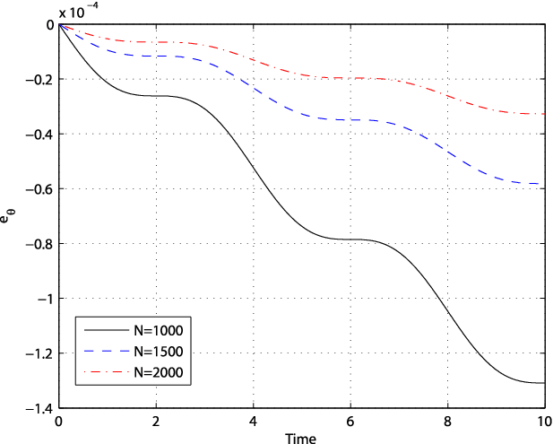
To verify the accuracy of our numerical computation, we give the corresponding continuous-time equations of motion for the planar rigid body on SO​(2)\textsf{SO}(2) using equations (7). The Lie bracket on SO​(2)\textsf{SO}(2) is identically equal to zero. Hence, one can check that the equations (7) are given by θ˙=ω\dot{\theta}=\omega, ω˙=τI\dot{\omega}=\frac{\tau}{I}, where θ\theta, ω\omega and τ\tau are the continuous time angular position, velocity and torque, respectively. We integrate the equations using the torque τ⁡(t)=sin⁡(π​t2)\tau(t)=\sin\left(\frac{\pi t}{2}\right), t∈[0,T]t\in[0,T]. We use the following parameters for our simulations: T=10T=10, I=1I=1, θ⁡(0)=3\theta(0)=3, ω⁡(0)=4\omega(0)=4 and we try three different time steps corresponding to N=1000,1500,2000N=1000,1500,2000. The error between the continuous- and discrete-time values of θ\theta and ω\omega are given in Figure (1). Note that the accuracy of the simulation improves with increasing NN.

Refer to caption
Refer to caption
Figure 1. Error dynamics on SO​(2)\textsf{SO}(2).
Remark 3.1.

Note that the discrete-time equations (3.2) correspond to the Euler approximation for the equations of motion. This is a check that our method returns something familiar for a simple example as the planar rigid body. However, we emphasize that on SO​(3)\textsf{SO}(3) the discretization will not necessarily be equivalent to any of the classical discretization schemes. The discretization will generally result in a set of nonlinear implicit algebraic equations.

3.3. Discrete-Time Variational Optimal Control Problem

We now address Problem 3.2 by first forming the appended cost functional:

𝒥\displaystyle\mathcal{J} =\displaystyle= ∑k=0N12≪𝝉k,𝝉k≫∗\displaystyle\sum_{k=0}^{N}\frac{1}{2}\ll\boldsymbol{\tau}_{k},\boldsymbol{\tau}_{k}\gg_{*}
+∑k=0N−1⟨𝚲k1,−h𝛀k+exp−1(𝐑k−1𝐑k+1)⟩\displaystyle+\sum_{k=0}^{N-1}\left<\mathbf{\Lambda}_{k}^{1},-h\mathbf{\Omega}_{k}+\exp^{-1}\left(\mathbf{R}^{-1}_{k}\mathbf{R}_{k+1}\right)\right>
+∑k=1N−1⟨𝐌k−Ad𝐠k∗(h𝝉k+𝐌k−1),𝚲k2⟩.\displaystyle+\sum_{k=1}^{N-1}\left<\mathbf{M}_{k}-{\rm Ad}_{\mathbf{g}_{k}}^{*}\left(h\boldsymbol{\tau}_{k}+\mathbf{M}_{k-1}\right),\mathbf{\Lambda}_{k}^{2}\right>.

Writing 𝐌k=Ad𝐠k∗​(h​𝝉k+𝐌k−1)\mathbf{M}_{k}={\rm Ad}_{\mathbf{g}_{k}}^{*}\left(h\boldsymbol{\tau}_{k}+\mathbf{M}_{k-1}\right) as 𝐌k=𝐠k−1​(h​𝝉k+𝐌k−1)​𝐠k\mathbf{M}_{k}=\mathbf{g}_{k}^{-1}\left(h\boldsymbol{\tau}_{k}+\mathbf{M}_{k-1}\right)\mathbf{g}_{k} and taking variations of this expression, we obtain

𝜹​𝐌k\displaystyle\boldsymbol{\delta}\mathbf{M}_{k} =\displaystyle= −h​𝜹​𝛀k​𝐠k−1​(h​𝝉k+𝐌k−1)​𝐠k\displaystyle-h\boldsymbol{\delta}\mathbf{\Omega}_{k}\mathbf{g}_{k}^{-1}\left(h\boldsymbol{\tau}_{k}+\mathbf{M}_{k-1}\right)\mathbf{g}_{k}
+𝐠k−1​(h​𝜹​𝝉k+𝜹​𝐌k−1)​𝐠k\displaystyle+\mathbf{g}_{k}^{-1}\left(h\boldsymbol{\delta}\boldsymbol{\tau}_{k}+\boldsymbol{\delta}\mathbf{M}_{k-1}\right)\mathbf{g}_{k}
+h​𝐠k−1​(h​𝝉k+𝐌k−1)​𝐠k​𝜹​𝛀k\displaystyle+h\mathbf{g}_{k}^{-1}\left(h\boldsymbol{\tau}_{k}+\mathbf{M}_{k-1}\right)\mathbf{g}_{k}\boldsymbol{\delta}\mathbf{\Omega}_{k}
=\displaystyle= −h​𝜹​𝛀k​𝐌k+Ad𝐠k∗​(h​𝜹​𝝉k+𝐉⁡(𝜹​𝛀k−1))\displaystyle-h\boldsymbol{\delta}\mathbf{\Omega}_{k}\mathbf{M}_{k}+{\rm Ad}^{*}_{\mathbf{g}_{k}}\left(h\boldsymbol{\delta}\boldsymbol{\tau}_{k}+\mathbf{J}\left(\boldsymbol{\delta}\mathbf{\Omega}_{k-1}\right)\right)
+h​𝐌k​𝜹​𝛀k\displaystyle+h\mathbf{M}_{k}\boldsymbol{\delta}\mathbf{\Omega}_{k}
=\displaystyle= Ad𝐠k∗​(h​𝜹​𝝉k+𝐉⁡(𝜹​𝛀k−1))+h⁡[𝐌k,𝜹​𝛀k].\displaystyle{\rm Ad}_{\mathbf{g}_{k}}^{*}\left(h\boldsymbol{\delta}\boldsymbol{\tau}_{k}+\mathbf{J}\left(\boldsymbol{\delta}\mathbf{\Omega}_{k-1}\right)\right)+h\left[\mathbf{M}_{k},\boldsymbol{\delta}\mathbf{\Omega}_{k}\right].

In obtaining this expression we used the facts that 𝜹​𝐠k=h​𝐠k​𝜹​𝛀k\boldsymbol{\delta}\mathbf{g}_{k}=h\mathbf{g}_{k}\boldsymbol{\delta}\mathbf{\Omega}_{k} and 𝜹⁡(𝐠k−1)=−h​𝜹​𝛀k​𝐠k−1\boldsymbol{\delta}\left(\mathbf{g}_{k}^{-1}\right)=-h\boldsymbol{\delta}\mathbf{\Omega}_{k}\mathbf{g}_{k}^{-1}. The latter equality is obtained as follows. Taking variations of (𝐠kϵ)−1​(𝐠kϵ)=𝐈\left(\mathbf{g}_{k}^{\epsilon}\right)^{-1}\left(\mathbf{g}_{k}^{\epsilon}\right)=\mathbf{I}, we obtain

0\displaystyle 0 =\displaystyle= 𝜹⁡(𝐠k−1)​𝐠k+h​𝐠k−1​𝐠k​𝜹​𝛀k\displaystyle\boldsymbol{\delta}\left(\mathbf{g}_{k}^{-1}\right)\mathbf{g}_{k}+h\mathbf{g}_{k}^{-1}\mathbf{g}_{k}\boldsymbol{\delta}\mathbf{\Omega}_{k}

which implies that

𝜹⁡(𝐠k−1)=−h​𝜹​𝛀k​𝐠k−1,\displaystyle\boldsymbol{\delta}\left(\mathbf{g}_{k}^{-1}\right)=-h\boldsymbol{\delta}\mathbf{\Omega}_{k}\mathbf{g}_{k}^{-1},

which is the desired result.

We now also consider the velocity boundary conditions 𝛀0=𝛀0∗\mathbf{\Omega}_{0}=\mathbf{\Omega}_{0}^{*} and 𝛀N−1=𝛀N−1∗\mathbf{\Omega}_{N-1}=\mathbf{\Omega}_{N-1}^{*}. Note that variations in 𝜹​𝛀k\boldsymbol{\delta}\mathbf{\Omega}_{k} directly induce variations in 𝐖k+1\mathbf{W}_{k+1}. In particular, if k=0k=0 and we have the initial constraints 𝐑0=𝐑0∗\mathbf{R}_{0}=\mathbf{R}_{0}^{*} and 𝛀0=𝛀0∗\mathbf{\Omega}_{0}=\mathbf{\Omega}_{0}^{*}, then 𝐖0=0\mathbf{W}_{0}=0 and 𝜹​𝛀0=0\boldsymbol{\delta}\mathbf{\Omega}_{0}=0. Using these two equations in equation (23), we find that

(36) 𝐖1=0.\displaystyle\mathbf{W}_{1}=0.

At k=N,N−1k=N,N-1, the constraints 𝐑N=𝐑N∗\mathbf{R}_{N}=\mathbf{R}_{N}^{*} and 𝛀N−1=𝛀N−1∗\mathbf{\Omega}_{N-1}=\mathbf{\Omega}_{N-1}^{*} imply that 𝐖N=0\mathbf{W}_{N}=0 and 𝜹​𝛀N−1=0\boldsymbol{\delta}\mathbf{\Omega}_{N-1}=0. Using these two equations in equation (23), we find that

(37) 𝐖N−1=0.\displaystyle\mathbf{W}_{N-1}=0.

The observations stated in equations (36) and (37) are equivalent to having

(38) 𝐑1=𝐑0∗​exp⁡(h​𝛀0∗),𝐑N−1=𝐑N∗​exp⁡(−h​𝛀N−1∗).\displaystyle\mathbf{R}_{1}=\mathbf{R}_{0}^{*}\exp\left(h\mathbf{\Omega}_{0}^{*}\right),~\mathbf{R}_{N-1}=\mathbf{R}_{N}^{*}\exp\left(-h\mathbf{\Omega}_{N-1}^{*}\right).

Taking variations of the cost functional, we obtain

𝜹​𝒥=∑k=0N⟨𝜹​𝝉k,𝝉k♯⟩\displaystyle\boldsymbol{\delta}\mathcal{J}=\sum_{k=0}^{N}\left<\boldsymbol{\delta}\boldsymbol{\tau}_{k},\boldsymbol{\tau}_{k}^{\sharp}\right>
+∑k=0N−1⟨𝚲k1,−𝜹𝛀k+1h[−Ad𝐠k−1𝐖k+𝐖k+1]⟩\displaystyle+\sum_{k=0}^{N-1}\bigg<\mathbf{\Lambda}_{k}^{1},-\boldsymbol{\delta}\mathbf{\Omega}_{k}+\frac{1}{h}\left[-{\rm Ad}_{\mathbf{g}_{k}^{-1}}\mathbf{W}_{k}+\mathbf{W}_{k+1}\right]\bigg>
+∑k=1N−1⟨𝐉(𝜹𝛀k)−Ad𝐠k∗(h𝜹𝝉k+𝐉(𝜹𝛀k−1))\displaystyle+\sum_{k=1}^{N-1}\big<\mathbf{J}\left(\boldsymbol{\delta}\mathbf{\Omega}_{k}\right)-{\rm Ad}_{\mathbf{g}_{k}}^{*}\left(h\boldsymbol{\delta}\boldsymbol{\tau}_{k}+\mathbf{J}\left(\boldsymbol{\delta}\mathbf{\Omega}_{k-1}\right)\right)
−h⁡[𝐌k,𝜹​𝛀k],𝚲k2⟩,\displaystyle\hskip 36.135pt-h\left[\mathbf{M}_{k},\boldsymbol{\delta}\mathbf{\Omega}_{k}\right],\mathbf{\Lambda}_{k}^{2}\big>,

where we have replaced 𝜹​𝐌k\boldsymbol{\delta}\mathbf{M}_{k} with 𝐉⁡(𝜹​𝛀k)\mathbf{J}\left(\boldsymbol{\delta}\mathbf{\Omega}_{k}\right). Collecting terms, setting 𝜹​𝒥\boldsymbol{\delta}\mathcal{J} to zero, and using the conditions 𝐖0=𝐖1=𝐖N−1=𝐖N=𝜹​𝛀0=𝜹​𝛀N−1=0\mathbf{W}_{0}=\mathbf{W}_{1}=\mathbf{W}_{N-1}=\mathbf{W}_{N}=\boldsymbol{\delta}\mathbf{\Omega}_{0}=\boldsymbol{\delta}\mathbf{\Omega}_{N-1}=0 and the fact that 𝐉⁡(⋅)\mathbf{J}(\cdot) is self-adjoint, we obtain the following theorem.

Theorem 3.1.

The necessary optimality conditions for the discrete Problem 3.2 are

𝐑k+1\displaystyle\mathbf{R}_{k+1} =\displaystyle= 𝐑k​𝐠k,k=1,…,N−2\displaystyle\mathbf{R}_{k}\mathbf{g}_{k},~k=1,\ldots,N-2
𝐌k\displaystyle\mathbf{M}_{k} =\displaystyle= Ad𝐠k∗​(h​𝝉k+𝐌k−1),k=1,…,N−1\displaystyle{\rm Ad}_{\mathbf{g}_{k}}^{*}\left(h\boldsymbol{\tau}_{k}+\mathbf{M}_{k-1}\right),~k=1,\ldots,N-1
0\displaystyle 0 =\displaystyle= 𝚲k−11−Ad𝐠k−1∗​𝚲k1,k=2,…,N−2\displaystyle\mathbf{\Lambda}_{k-1}^{1}-{\rm Ad}_{\mathbf{g}_{k}^{-1}}^{*}\mathbf{\Lambda}_{k}^{1},~k=2,\ldots,N-2
(39) 0\displaystyle 0 =\displaystyle= −𝚲k1+𝐉⁡(𝚲k2)−𝐉⁡(Ad𝐠k+1​𝚲k+12)\displaystyle-\mathbf{\Lambda}_{k}^{1}+\mathbf{J}\left(\mathbf{\Lambda}_{k}^{2}\right)-\mathbf{J}\left({\rm Ad}_{\mathbf{g}_{k+1}}\mathbf{\Lambda}_{k+1}^{2}\right)
+h⁡[𝐌k,𝚲k2],k=1,…,N−2\displaystyle+h\left[\mathbf{M}_{k},\mathbf{\Lambda}_{k}^{2}\right],~k=1,\ldots,N-2
𝝉k\displaystyle\boldsymbol{\tau}_{k} =\displaystyle= h​(Ad𝐠k​𝚲k2)♭,k=1,…,N−1\displaystyle h\left({\rm Ad}_{\mathbf{g}_{k}}\mathbf{\Lambda}_{k}^{2}\right)^{\flat},~k=1,\ldots,N-1
𝐌k\displaystyle\mathbf{M}_{k} =\displaystyle= 𝐉⁡(𝛀k),k=0,…,N−1,\displaystyle\mathbf{J}\left(\mathbf{\Omega}_{k}\right),~k=0,\ldots,N-1,

and the boundary conditions

𝐑0\displaystyle\mathbf{R}_{0} =\displaystyle= 𝐑0∗,𝐑1=𝐑0∗​𝐠0∗,𝛀0=𝛀0∗\displaystyle\mathbf{R}_{0}^{*},~\mathbf{R}_{1}=\mathbf{R}_{0}^{*}\mathbf{g}_{0}^{*},~\mathbf{\Omega}_{0}=\mathbf{\Omega}_{0}^{*}
𝐑N\displaystyle\mathbf{R}_{N} =\displaystyle= 𝐑N∗,𝐑N−1=𝐑N∗​(𝐠N−1∗)−1,𝛀N−1=𝛀N−1∗\displaystyle\mathbf{R}_{N}^{*},~\mathbf{R}_{N-1}=\mathbf{R}_{N}^{*}\left(\mathbf{g}_{N-1}^{*}\right)^{-1},~\mathbf{\Omega}_{N-1}=\mathbf{\Omega}_{N-1}^{*}
𝝉0\displaystyle\boldsymbol{\tau}_{0} =\displaystyle= 𝝉N=0,\displaystyle\boldsymbol{\tau}_{N}=0,

where 𝐠0∗=exp⁡(h​𝛀0∗)\mathbf{g}_{0}^{*}=\exp(h\mathbf{\Omega}_{0}^{*}) and 𝐠N−1∗=exp⁡(h​𝛀N−1∗)\mathbf{g}_{N-1}^{*}=\exp\left(h\mathbf{\Omega}_{N-1}^{*}\right).

A Second Order Direct Approach.

Analogous to the direct approach in continuous time, here we derive the necessary optimality conditions in a form that does not involve the use of Lagrange multipliers. Using equation (23) and taking variation of the second of equations (1), we obtain

(40) 𝜹​𝝉k\displaystyle\boldsymbol{\delta}\boldsymbol{\tau}_{k} =\displaystyle= Ad𝐠k−1∗​(1h2​𝐉​(𝐖k+1−Ad𝐠k−1​𝐖k)CLOSE\displaystyle{\rm Ad}^{*}_{\mathbf{g}_{k}^{-1}}\bigg(\frac{1}{h^{2}}\mathbf{J}\left(\mathbf{W}_{k+1}-{\rm Ad}_{\mathbf{g}_{k}^{-1}}\mathbf{W}_{k}\right)
OPEN+1h​[𝐖k+1−Ad𝐠k−1​𝐖k,𝐉⁡(𝛀k)])\displaystyle+\frac{1}{h}\left[\mathbf{W}_{k+1}-{\rm Ad}_{\mathbf{g}_{k}^{-1}}\mathbf{W}_{k},\mathbf{J}\left(\mathbf{\Omega}_{k}\right)\right]\bigg)
−1h2​𝐉​(𝐖k−Ad𝐠k−1−1​𝐖k−1),\displaystyle-\frac{1}{h^{2}}\mathbf{J}\left(\mathbf{W}_{k}-{\rm Ad}_{\mathbf{g}_{k-1}^{-1}}\mathbf{W}_{k-1}\right),

for k=1,…,N−1k=1,\ldots,N-1. Taking variations of the cost functional (18) and substituting from equation (40) one obtains after a tedious but straight forward computation an expression for 𝜹​𝒥\boldsymbol{\delta}\mathcal{J} in terms of 𝜹​𝝉k\boldsymbol{\delta}\boldsymbol{\tau}_{k}:

𝜹​𝒥\displaystyle\boldsymbol{\delta}\mathcal{J} =\displaystyle= ∑k=1N−1[⟨Ad𝐠k−1∗(1h2𝐉(𝐖k+1−Ad𝐠k−1𝐖k)\displaystyle\sum_{k=1}^{N-1}\Bigg[\big<{\rm Ad}^{*}_{\mathbf{g}_{k}^{-1}}\bigg(\frac{1}{h^{2}}\mathbf{J}\left(\mathbf{W}_{k+1}-{\rm Ad}_{\mathbf{g}_{k}^{-1}}\mathbf{W}_{k}\right)
+1h[𝐖k+1−Ad𝐠k−1𝐖k,𝐉(𝛀k)])−1h2𝐉(𝐖k−Ad𝐠k−1−1𝐖k−1),𝝉k♯⟩]\displaystyle+\frac{1}{h}\left[\mathbf{W}_{k+1}-{\rm Ad}_{\mathbf{g}_{k}^{-1}}\mathbf{W}_{k},\mathbf{J}\left(\mathbf{\Omega}_{k}\right)\right]\bigg)-\frac{1}{h^{2}}\mathbf{J}\left(\mathbf{W}_{k}-{\rm Ad}_{\mathbf{g}_{k-1}^{-1}}\mathbf{W}_{k-1}\right),\boldsymbol{\tau}^{\sharp}_{k}\big>\Bigg]
+⟨𝜹​𝝉0,𝝉0♯⟩+⟨𝜹​𝝉N,𝝉N♯⟩.\displaystyle+\left<\boldsymbol{\delta}\boldsymbol{\tau}_{0},\boldsymbol{\tau}_{0}^{\sharp}\right>+\left<\boldsymbol{\delta}\boldsymbol{\tau}_{N},\boldsymbol{\tau}_{N}^{\sharp}\right>.

When 𝜹​𝒥\boldsymbol{\delta}\mathcal{J} is equated to zero (and after some algebraic rearrangement), one can obtain the boundary conditions on 𝝉0,𝝉1,𝝉N−1,𝝉N\boldsymbol{\tau}_{0},\boldsymbol{\tau}_{1},\boldsymbol{\tau}_{N-1},\boldsymbol{\tau}_{N} from the resulting equations below:

𝝉0\displaystyle\boldsymbol{\tau}_{0} =\displaystyle= 0\displaystyle 0
0\displaystyle 0 =\displaystyle= −1h2​(𝐉⁡(𝝉1♯)+Ad𝐠1−1∗​𝐉​(Ad𝐠1−1​𝝉1♯))\displaystyle-\frac{1}{h^{2}}\left(\mathbf{J}\left(\boldsymbol{\tau}_{1}^{\sharp}\right)+{\rm Ad}^{*}_{\mathbf{g}_{1}^{-1}}\mathbf{J}\left({\rm Ad}_{\mathbf{g}_{1}^{-1}}\boldsymbol{\tau}_{1}^{\sharp}\right)\right)
−1h​Ad𝐠1−1∗​[𝐉⁡(𝛀1),Ad𝐠1−1​(𝝉1♯)]\displaystyle-\frac{1}{h}{\rm Ad}^{*}_{\mathbf{g}_{1}^{-1}}\left[\mathbf{J}\left(\mathbf{\Omega}_{1}\right),{\rm Ad}_{\mathbf{g}_{1}^{-1}}\left(\boldsymbol{\tau}_{1}^{\sharp}\right)\right]
0\displaystyle 0 =\displaystyle= −1h2​(𝐉⁡(𝝉N−1♯)+Ad𝐠N−1−1∗​𝐉​(Ad𝐠N−1−1​𝝉N−1♯))\displaystyle-\frac{1}{h^{2}}\left(\mathbf{J}\left(\boldsymbol{\tau}_{N-1}^{\sharp}\right)+{\rm Ad}^{*}_{\mathbf{g}_{N-1}^{-1}}\mathbf{J}\left({\rm Ad}_{\mathbf{g}_{N-1}^{-1}}\boldsymbol{\tau}_{N-1}^{\sharp}\right)\right)
−1h​Ad𝐠N−1−1∗​[𝐉⁡(𝛀N−1),Ad𝐠N−1−1​(𝝉N−1♯)]\displaystyle-\frac{1}{h}{\rm Ad}^{*}_{\mathbf{g}_{N-1}^{-1}}\left[\mathbf{J}\left(\mathbf{\Omega}_{N-1}\right),{\rm Ad}_{\mathbf{g}_{N-1}^{-1}}\left(\boldsymbol{\tau}_{N-1}^{\sharp}\right)\right]
𝝉N\displaystyle\boldsymbol{\tau}_{N} =\displaystyle= 0\displaystyle 0

as well as discrete evolution equations that are written in algebraic nonlinear form as:

(41) 0\displaystyle 0 =\displaystyle= −1h2​(𝐉⁡(𝝉k♯)−Ad𝐠k−1∗​𝐉​(𝝉k+1♯)CLOSE\displaystyle-\frac{1}{h^{2}}\bigg(\mathbf{J}\left(\boldsymbol{\tau}_{k}^{\sharp}\right)-{\rm Ad}^{*}_{\mathbf{g}_{k}^{-1}}\mathbf{J}\left(\boldsymbol{\tau}_{k+1}^{\sharp}\right)
OPEN−𝐉⁡(Ad𝐠k−1−1​𝝉k−1♯)+Ad𝐠k−1∗​𝐉​(Ad𝐠k−1​𝝉k♯))\displaystyle-\mathbf{J}\left({\rm Ad}_{\mathbf{g}_{k-1}^{-1}}\boldsymbol{\tau}_{k-1}^{\sharp}\right)+{\rm Ad}^{*}_{\mathbf{g}_{k}^{-1}}\mathbf{J}\left({\rm Ad}_{\mathbf{g}_{k}^{-1}}\boldsymbol{\tau}_{k}^{\sharp}\right)\bigg)
−1h​(Ad𝐠k−1∗​[𝐉⁡(𝛀k),Ad𝐠k−1​(𝝉k♯)]CLOSE\displaystyle-\frac{1}{h}\bigg({\rm Ad}^{*}_{\mathbf{g}_{k}^{-1}}\left[\mathbf{J}\left(\mathbf{\Omega}_{k}\right),{\rm Ad}_{\mathbf{g}_{k}^{-1}}\left(\boldsymbol{\tau}_{k}^{\sharp}\right)\right]
OPEN−1h​[𝐉⁡(𝛀k−1),Ad𝐠k−1−1​(𝝉k−1♯)]),\displaystyle-\frac{1}{h}\left[\mathbf{J}\left(\mathbf{\Omega}_{k-1}\right),{\rm Ad}_{\mathbf{g}_{k-1}^{-1}}\left(\boldsymbol{\tau}_{k-1}^{\sharp}\right)\right]\bigg),

for k=2,…,N−2k=2,\ldots,N-2.

The following section shows that while our discrete approximation (14) is formally first-order accurate, it is symplectically equivalent to the second-order accurate Störmer–Verlet method, and hence has effective order two.

4. Lie Symplectic Euler and Symplectic Equivalence

Notice that the discrete Lagrangian adopted in our paper is obtained by approximating the velocity as a constant over the timestep hh, and by approximating the integral in time by ∫t1t2f⁡(t)​𝑑t≈(t2−t1)​f​(t1)\int_{t_{1}}^{t_{2}}f(t)dt\approx(t_{2}-t_{1})f(t_{1}). In the Lie group setting, the constant angular velocity approximation corresponds to the condition,

𝐑k+1=𝐑k​exp⁡(h​𝛀k)\mathbf{R}_{k+1}=\mathbf{R}_{k}\exp(h\mathbf{\Omega}_{k})

or equivalently,

𝛀k=1h​exp−1⁡(𝐑k−1​𝐑k+1).\mathbf{\Omega}_{k}=\frac{1}{h}\exp^{-1}(\mathbf{R}_{k}^{-1}\mathbf{R}_{k+1}).

When we let G=ℝnG=\mathbb{R}^{n}, and we adopt the notation (𝐪,𝐯)∈T​ℝn(\mathbf{q},\mathbf{v})\in T\mathbb{R}^{n}, we obtain,

𝐯k=𝐪k+1−𝐪kh,\mathbf{v}_{k}=\frac{\mathbf{q}_{k+1}-\mathbf{q}_{k}}{h},

which is a usual finite-difference approximation for the velocity. Consider then a Lagrangian of the form,

L⁡(𝐪,𝐯)=12​𝐯T​M​𝐯−V⁡(𝐪).L(\mathbf{q},\mathbf{v})=\frac{1}{2}\mathbf{v}^{T}M\mathbf{v}-V(\mathbf{q}).

Approximating the action integral from 00 to hh using a constant velocity approximation and a quadrature formula, yields,

∫0hL⁡(𝐪⁡(t),𝐯⁡(t))​𝑑t≈∫0hL⁡(𝐪⁡(t),𝐪k+1−𝐪kh)​𝑑t≈h​L​(𝐪k,𝐪k+1−𝐪kh).\int_{0}^{h}L(\mathbf{q}(t),\mathbf{v}(t))dt\approx\int_{0}^{h}L\Bigl(\mathbf{q}(t),\frac{\mathbf{q}_{k+1}-\mathbf{q}_{k}}{h}\Bigr)dt\approx hL\Bigl(\mathbf{q}_{k},\frac{\mathbf{q}_{k+1}-\mathbf{q}_{k}}{h}\Bigr).

We then choose as our discrete Lagrangian,

Ld​(𝐪k,𝐪k+1)=h​L​(𝐪k,𝐪k+1−𝐪kh)=h⁡[12​(𝐪k+1−𝐪kh)T​M​(𝐪k+1−𝐪kh)−V⁡(𝐪k)].L_{d}(\mathbf{q}_{k},\mathbf{q}_{k+1})=hL\Bigl(\mathbf{q}_{k},\frac{\mathbf{q}_{k+1}-\mathbf{q}_{k}}{h}\Bigr)=h\left[\frac{1}{2}\Bigl(\frac{\mathbf{q}_{k+1}-\mathbf{q}_{k}}{h}\Bigr)^{T}M\Bigl(\frac{\mathbf{q}_{k+1}-\mathbf{q}_{k}}{h}\Bigr)-V(\mathbf{q}_{k})\right].

The discrete Euler–Lagrange equations,

D2​Ld​(𝐪k−1,𝐪k)+D1​Ld​(𝐪k,𝐪k+1)=0,D_{2}L_{d}(\mathbf{q}_{k-1},\mathbf{q}_{k})+D_{1}L_{d}(\mathbf{q}_{k},\mathbf{q}_{k+1})=0,

yields,

M⁡(𝐪k−𝐪k−1h)−M⁡(𝐪k+1−𝐪kh)−h​∂V∂𝐪​(𝐪k)=0,M\Bigl(\frac{\mathbf{q}_{k}-\mathbf{q}_{k-1}}{h}\Bigr)-M\Bigl(\frac{\mathbf{q}_{k+1}-\mathbf{q}_{k}}{h}\Bigr)-h\frac{\partial V}{\partial\mathbf{q}}(\mathbf{q}_{k})=0,

which induces an implicit update map (𝐪k−1,𝐪k)↦(𝐪k,𝐪k+1)(\mathbf{q}_{k-1},\mathbf{q}_{k})\mapsto(\mathbf{q}_{k},\mathbf{q}_{k+1}). To obtain the corresponding Hamiltonian update map, we push-forward this algorithm to T∗​QT^{*}Q by using the discrete fiber derivative 𝔽​Ld:Q×Q→T∗​Q\mathbb{F}L_{d}:Q\times Q\rightarrow T^{*}Q, which takes (𝐪k,𝐪k+1)↦(𝐪k+1,D2​Ld​(𝐪k,𝐪k+1))(\mathbf{q}_{k},\mathbf{q}_{k+1})\mapsto(\mathbf{q}_{k+1},D_{2}L_{d}(\mathbf{q}_{k},\mathbf{q}_{k+1})). In particular, we have that,

𝐩k+1=D2​Ld​(𝐪k,𝐪k+1)=M⁡(𝐪k+1−𝐪kh),\mathbf{p}_{k+1}=D_{2}L_{d}(\mathbf{q}_{k},\mathbf{q}_{k+1})=M\Bigl(\frac{\mathbf{q}_{k+1}-\mathbf{q}_{k}}{h}\Bigr),

which implies

(42) 𝐪k+1=𝐪k+h​M−1​𝐩k+1.\displaystyle\mathbf{q}_{k+1}=\mathbf{q}_{k}+hM^{-1}\mathbf{p}_{k+1}.

This allows us to rewrite the discrete Euler–Lagrange equations as,

𝐩k−𝐩k+1−h​∂V∂q​(𝐪k)=0,\mathbf{p}_{k}-\mathbf{p}_{k+1}-h\frac{\partial V}{\partial q}(\mathbf{q}_{k})=0,

or equivalently,

(43) 𝐩k+1=𝐩k−h​∂V∂q​(𝐪k).\displaystyle\mathbf{p}_{k+1}=\mathbf{p}_{k}-h\frac{\partial V}{\partial q}(\mathbf{q}_{k}).

Now, (42) and (43) are precisely the symplectic Euler method applied to the corresponding Hamiltonian vector field, as we shall see.

The corresponding Hamiltonian is given by,

H⁡(𝐪,𝐩)=12​𝐩T​M−1​𝐩+V⁡(𝐪).H(\mathbf{q},\mathbf{p})=\frac{1}{2}\mathbf{p}^{T}M^{-1}\mathbf{p}+V(\mathbf{q}).

Hamilton’s equations yield,

(𝐪˙𝐩˙)=(∂H∂𝐩−∂H∂𝐪)=(M−1​𝐩−∂V∂𝐪).\begin{pmatrix}\dot{\mathbf{q}}\\ \dot{\mathbf{p}}\end{pmatrix}=\begin{pmatrix}\frac{\partial H}{\partial\mathbf{p}}\\ -\frac{\partial H}{\partial\mathbf{q}}\end{pmatrix}=\begin{pmatrix}M^{-1}\mathbf{p}\\ -\frac{\partial V}{\partial\mathbf{q}}\end{pmatrix}.

The symplectic Euler method has the form,

𝐪k+1\displaystyle\mathbf{q}_{k+1} =𝐪k+h​𝐪˙​(𝐪k,𝐩k+1),\displaystyle=\mathbf{q}_{k}+h\dot{\mathbf{q}}(\mathbf{q}_{k},\mathbf{p}_{k+1}),
𝐩k+1\displaystyle\mathbf{p}_{k+1} =𝐩k+h​𝐩˙​(𝐪k,𝐩k+1),\displaystyle=\mathbf{p}_{k}+h\dot{\mathbf{p}}(\mathbf{q}_{k},\mathbf{p}_{k+1}),
which yields,
𝐪k+1\displaystyle\mathbf{q}_{k+1} =𝐪k+h​M−1​𝐩k+1,\displaystyle=\mathbf{q}_{k}+hM^{-1}\mathbf{p}_{k+1},
𝐩k+1\displaystyle\mathbf{p}_{k+1} =𝐩k+h⁡(−∂V∂q​(𝐪k)),\displaystyle=\mathbf{p}_{k}+h\left(-\frac{\partial V}{\partial q}(\mathbf{q}_{k})\right),

which is precisely what we obtained in (42) and (43). This demonstrates that our method is the generalization of the symplectic Euler method to Lie groups, which has important numerical consequences. While symplectic Euler is formally first-order accurate, it is symplectically equivalent [27, 18] to the second-order accurate Störmer–Verlet method [6]. This means that one can obtain the Störmer–Verlet method FSVF_{\rm SV} by conjugating the symplectic Euler method FEF_{\rm E} with a symplectic transformation TT,

FSV=T​FE​T−1.F_{\rm SV}=TF_{\rm E}T^{-1}.

In particular, numerical trajectories of symplectic Euler will shadow numerical trajectories obtained using Störmer–Verlet. Consider the implications of this symplectic equivalence for our discrete optimal control problem. Let the boundary conditions be specified by 𝐪0,𝐪N\mathbf{q}_{0},\mathbf{q}_{N}, and assume that we use Störmer–Verlet to propagate the solution, then the boundary condition is expressed as, 𝐪N=FSVN​𝐪0=(T​FE​T−1)N​𝐪0=T​FEN​T−1​𝐪0,\mathbf{q}_{N}=F_{\rm SV}^{N}\mathbf{q}_{0}=(TF_{\rm E}T^{-1})^{N}\mathbf{q}_{0}=TF_{\rm E}^{N}T^{-1}\mathbf{q}_{0}, which is equivalent to q~N=T−1​𝐪N=FEN​T−1​𝐪0=FEN​q~0\tilde{q}_{N}=T^{-1}\mathbf{q}_{N}=F_{\rm E}^{N}T^{-1}\mathbf{q}_{0}=F_{\rm E}^{N}\tilde{q}_{0}. This implies that if we preprocess the boundary conditions 𝐪0,𝐪N\mathbf{q}_{0},\mathbf{q}_{N}, to obtain q~0=T−1​𝐪0,q~N=T−1​𝐪N\tilde{q}_{0}=T^{-1}\mathbf{q}_{0},\tilde{q}_{N}=T^{-1}\mathbf{q}_{N}, we could use symplectic Euler at the internal stages to propagate the states and costates, and then postprocess them to obtain the trajectory one would have obtained by using Störmer–Verlet.

In practice, the shadowing result imparts the symplectic Euler method with the same desirable qualitative properties as Störmer–Verlet, and it is not necessary to postprocess the numerical solutions in order to achieve accurate results. Since on an appropriate choice of charts, our Lie symplectic Euler method reduces to symplectic Euler in coordinates, it follows that there is a corresponding second-order Lie Störmer–Verlet method that our method is symplectically equivalent to, and in particular, our method has effective order two.

5. Numerical Approach and Results

The multiplier-free version of the first-order optimality equations, equation (41), in combination with the boundary conditions,

𝐑0=𝐑0∗,𝐑N=𝐑N∗,𝛀0=𝛀0∗,and ​𝛀N−1=𝛀N−1∗,\mathbf{R}_{0}=\mathbf{R}_{0}^{*},\;\ \mathbf{R}_{N}=\mathbf{R}_{N}^{*},\;\ \mathbf{\Omega}_{0}=\mathbf{\Omega}_{0}^{*},\;\ \mbox{and }\mathbf{\Omega}_{N-1}=\mathbf{\Omega}_{N-1}^{*},

leave the torques 𝝉1,…,𝝉N−1\boldsymbol{\tau}_{1},\ldots,\boldsymbol{\tau}_{N-1}, and the angular velocities 𝛀1,…,𝛀N−2\mathbf{\Omega}_{1},\ldots,\mathbf{\Omega}_{N-2} as unknowns. By substituting the relations 𝐠k=exp⁡(h​𝛀k)\mathbf{g}_{k}=\exp(h\mathbf{\Omega}_{k}), 𝐌k=𝐉⁡(𝛀k)\mathbf{M}_{k}=\mathbf{J}(\mathbf{\Omega}_{k}), we can rewrite the necessary conditions (41) as follows,

0=\displaystyle 0= −1h2​(𝐉⁡(𝝉k♯)−Adexp⁡(−h​𝛀k)∗​𝐉​(𝝉k+1♯)CLOSE\displaystyle-\frac{1}{h^{2}}\Big(\mathbf{J}(\boldsymbol{\tau}^{\sharp}_{k})-{\rm Ad}^{*}_{\exp(-h\mathbf{\Omega}_{k})}\mathbf{J}(\boldsymbol{\tau}^{\sharp}_{k+1})
−𝐉⁡(Adexp⁡(−h​𝛀k−1)​𝝉k−1♯CLOSE\displaystyle\qquad\qquad-\mathbf{J}({\rm Ad}_{\exp(-h\mathbf{\Omega}_{k-1})}\boldsymbol{\tau}^{\sharp}_{k-1}
OPEN+Adexp⁡(−h​𝛀k)∗​𝐉​(Adexp⁡(−h​𝛀k)​𝝉k♯))\displaystyle\qquad\qquad+{\rm Ad}^{*}_{\exp(-h\mathbf{\Omega}_{k})}\mathbf{J}({\rm Ad}_{\exp(-h\mathbf{\Omega}_{k})}\boldsymbol{\tau}^{\sharp}_{k})\Big)
−1h​(Adexp⁡(−h​𝛀k)∗​[𝐉⁡(𝛀k),Adexp⁡(−h​𝛀k)​(𝝉k♯)]CLOSE\displaystyle-\frac{1}{h}\Big({\rm Ad}^{*}_{\exp(-h\mathbf{\Omega}_{k})}\Big[\mathbf{J}(\mathbf{\Omega}_{k}),{\rm Ad}_{\exp(-h\mathbf{\Omega}_{k})}(\boldsymbol{\tau}^{\sharp}_{k})\Big]
OPEN−1h​[𝐉⁡(𝛀k−1),Adexp⁡(−h​𝛀k−1)​(𝝉k−1♯)]),\displaystyle\qquad\qquad-\frac{1}{h}\Big[\mathbf{J}(\mathbf{\Omega}_{k-1}),{\rm Ad}_{\exp(-h\mathbf{\Omega}_{k-1})}(\boldsymbol{\tau}^{\sharp}_{k-1})\Big]\Big),
where k=2,…,N−2k=2,\ldots,N-2, and the discrete evolution equations, given by line 2 of (3.1), can be written as
0=\displaystyle 0= 𝐉⁡(𝛀k)−Adexp⁡(h​𝛀k)∗​(h​𝝉k+𝐉⁡(𝛀k−1)),\displaystyle\mathbf{J}(\mathbf{\Omega}_{k})-{\rm Ad}^{*}_{\exp(h\mathbf{\Omega}_{k})}(h\boldsymbol{\tau}_{k}+\mathbf{J}(\mathbf{\Omega}_{k-1})),
where k=1,…,N−1k=1,\ldots,N-1. In addition, we use the boundary conditions on 𝐑0\mathbf{R}_{0} and 𝐑N\mathbf{R}_{N}, together with the update step given by line 1 of (3.1) to give the last constraint,
0=\displaystyle 0= log⁡(𝐑N−1​𝐑0​exp⁡(h​𝛀0)​…​exp⁡(h​𝛀N−1)),\displaystyle\log\Big(\mathbf{R}_{N}^{-1}\mathbf{R}_{0}\exp(h\mathbf{\Omega}_{0})\ldots\exp(h\mathbf{\Omega}_{N-1})\Big),

where log\log is the logarithm map on SO​(3)\textsf{SO}(3).

Note that while we use the direct variational approach to obtain the discrete extremal solutions, an alternate way to obtain the discrete extremal solutions would be to use Pontryagin’s maximum principle. In particular, Bonnans and Laurent-Varin [4] show that these two approaches are equivalent in the context of symplectic partitioned Runge-Kutta schemes.

At this point it should be noted that one important advantage of the manner in which we have discretized the optimal control problem is that it is SO​(3)\textsf{SO}(3)-equivariant. This is to say that if we rotated all the boundary conditions by a fixed rotation matrix, and solved the resulting discrete optimal control problem, the solution we would obtain would simply be the rotation of the solution of the original problem. This can be seen quite clearly from the fact that the discrete problem is expressed in terms of body coordinates, both in terms of body angular velocities and body forces. In addition, the initial and final attitudes 𝐑0\mathbf{R}_{0} and 𝐑N\mathbf{R}_{N} only enter in the last equation as a relative rotation.

The SO​(3)\textsf{SO}(3)-equivariance of our numerical method is desirable, since it ensures that our results do not depend on the choice of coordinate frames. This is in contrast to methods based on coordinatizing the rotation group using quaternions and Euler angles.

Each of the equations above take values in 𝔰​𝔬​(3)\mathfrak{so}(3). Consider the Lie algebra isomorphism between ℝ3\mathbb{R}^{3} and 𝔰​𝔬​(3)\mathfrak{so}(3) given by the hat map,

𝐯=(v1,v2,v3)↦𝐯^=[0−v32v30−v1−v2v10],\mathbf{v}=(v_{1},v_{2},v_{3})\mapsto\hat{\mathbf{v}}=\begin{bmatrix}0&-v_{3}&{}_{2}\\ v_{3}&0&-v_{1}\\ -v_{2}&v_{1}&0\end{bmatrix},

which maps 3-vectors to 3×33\times 3 skew-symmetric matrices. In particular, we have the following identities,

[𝐮^,𝐯^]=(𝐮×𝐯)​^,Ad𝐀​𝐯^=(𝐀𝐯)​^.\displaystyle[\hat{\mathbf{u}},\hat{\mathbf{v}}]=(\mathbf{u}\times\mathbf{v})\,\hat{}\,,\quad{\rm Ad}_{\mathbf{A}}\hat{\mathbf{v}}=(\mathbf{A}\mathbf{v})\,\hat{}\,.

Furthermore, we identify 𝔰​𝔬​(3)∗\mathfrak{so}(3)^{*} with ℝ3\mathbb{R}^{3} by the usual dot product, that is to say if 𝚷\mathbf{\Pi}, 𝐯∈ℝ3\mathbf{v}\in\mathbb{R}^{3}, then ⟨𝚷,𝐯^⟩=𝚷⋅𝐯\langle\mathbf{\Pi},\hat{\mathbf{v}}\rangle=\mathbf{\Pi}\cdot\mathbf{v}. With this identification, we have that Ad𝐀−1∗​𝚷=𝐀​𝚷{\rm Ad}^{*}_{\mathbf{A}^{-1}}\mathbf{\Pi}=\mathbf{A}\mathbf{\Pi}. Using the identities above, we write the necessary conditions using matrix-vector products and cross products. Then, each of the equations can be interpreted as 33-vector valued functions, and the system of equations can be considered as a 3​(2​N−3)3(2N-3)-vector valued function, which is precisely the dimensionality of the unknowns. This reduces the discrete optimal problem to a nonlinear root finding problem.

The nonlinear system of equations was solved in MATLAB using the fsolve routine, where the Jacobian is constructed column by column, and the kk-th column is computed using the following approximation [19],

∂𝐅∂xk​(𝐱)=1ϵ​Im⁡[𝐅⁡(𝐱+i​ϵ​𝐞k)],\frac{\partial\mathbf{F}}{\partial x_{k}}(\mathbf{x})=\frac{1}{\epsilon}\operatorname{Im}[{\mathbf{F}(\mathbf{x}+i\epsilon\mathbf{e}_{k}})],

where i=−1i=\sqrt{-1}, 𝐞k\mathbf{e}_{k} is a basis vector in the xkx_{k} direction, and ϵ\epsilon is of the order of machine epsilon. This method is preferable to a finite-difference approximation, since it does not suffer from round-off errors, which would otherwise limit how small ϵ\epsilon can be.

Refer to caption
(a) Angular velocity and control torques
Refer to caption
(b) Principal axis and angle
Refer to caption
(c) Instantaneous rotation axis
Figure 2. Discrete optimal rest-to-rest maneuver in SO​(3)\textsf{SO}(3).

In our numerical simulation, we computed an optimal trajectory for a rest-to-rest maneuver, as illustrated in Figure (2). Here, the maneuver time is 12.8sec, N=128N=128, and the moment of inertia is given by

𝐉=[13.25−7.80−11.40−7.8016.254.71−11.404.7118.37].\mathbf{J}=\begin{bmatrix}13.25&-7.80&-11.40\\ -7.80&16.25&4.71\\ -11.40&4.71&18.37\end{bmatrix}.

The prescribed maneuver corresponds to a rotation by π3\frac{\pi}{3} about the xx-axis. Since the moment of inertia tensor is not a multiple of the identity, and the xx-axis does not correspond to the axis of minimal inertia, the optimal trajectory does not just involve a pure rotation about the xx-axis. It is worth noting that the results are not rotationally symmetric about the midpoint of the simulation interval, which is due to the fact that our choice of update, 𝐑k+1=𝐑k​exp⁡(h​𝛀k)\mathbf{R}_{k+1}=\mathbf{R}_{k}\exp(h\mathbf{\Omega}_{k}), does not exhibit time-reversal symmetry. In a forthcoming publication, we will introduce a reversible algorithm to address this issue. In particular, this will involve explicitly computing the stationarity conditions for the discrete optimal control problem constrained by the time-symmetric Lie Störmer–Verlet method.

Refer to caption
(a) Angular velocity and control torques
Refer to caption
(b) Principal axis and angle
Refer to caption
(c) Instantaneous rotation axis
Figure 3. Discrete optimal slew-up maneuver in SO​(3)\textsf{SO}(3).

We also present results for an optimal slew-up maneuver, illustrated in Figure (3). This uses the same moment of inertia tensor as in the previous simulation, and the desired maneuver involves a rotation of π6\frac{\pi}{6} about the xx-axis from rest to a final angular velocity of ΩN−1=[0.30.20.3]T\Omega_{N-1}=\begin{bmatrix}0.3&0.2&0.3\end{bmatrix}^{\mathrm{T}}, over a maneuver time of 12.8sec, and N=128N=128.

6. Conclusion

In this paper we studied the continuous- and discrete-time optimal control problem for the rigid body, where the cost to be minimized is the external torque applied to move the rigid body from an initial condition to some pre-specified terminal condition. In the discrete setting, we use the discrete Lagrange–d’Alembert principle to obtain the discrete equations of motion. The kinematics were discretized to guarantee that the flow in phase space remains on the Lie group SO​(3)\textsf{SO}(3) and its algebra 𝔰​𝔬​(3)\mathfrak{so}(3). We described how the necessary conditions can be solved for the general three-dimensional case and gave a numerical example for a three-dimensional rigid body maneuver.

The synthesis of variational mechanics with discrete-time optimal control is particularly advantageous from the point of view of computational efficiency, since the symplectic Euler method is symplectically conjugate to the Störmer–Verlet method, and hence has effective order two. Consequently, for our discrete-time optimal control method, the cost functional converges at a rate which is characteristic of a second-order method, while being based on a first-order method that is computationally cheaper.

Currently, we are investigating the use of the Pontryagin’s maximum principle with Lie group methods in continuous- and discrete-time to obtain the necessary conditions. Additionally, we wish to generalize the result to general Lie groups that have applications other than the rigid body motion on SO​(3)\textsf{SO}(3). In particular, we are interested in controlling the motion of a rigid body in space, which corresponds to motion on the non-compact Lie group SE​(3)\textsf{SE}(3).

Acknowledgments

The research of Islam Hussein was supported by a WPI Faculty Development Grant. The research of Melvin Leok was partially supported by NSF grants DMS-0504747 and DMS-0726263 and a University of Michigan Rackham faculty grant. The research of Anthony Bloch was supported by NSF grants DMS-030583, and CMS-0408542.

References

  • [1] New horizons: Pluto-kuiper belt mission. Website (2006). URL http://www.nasa.gov/mission_pages/newhorizons/main/index.html
  • [2] Agrachev, A.A., Sachkov, Y.: Control Theory from the Geometric Viewpoint. Springer-Verlag, New York, NY (2004)
  • [3] Bloch, A.: Nonholonomic Mechanics and Control. Springer-Verlag, New York, NY (2003)
  • [4] Bonnans, J., Laurent-Varin, J.: Computation of order conditions for symplectic partitioned runge-kutta schemes with application to optimal control. Num. Math. 103, 1–10 (2006)
  • [5] Hairer, E., Lubich, C., Wanner, G.: Geometric Numerical Integration. Springer, Berlin (2002)
  • [6] Hairer, E., Lubich, C., Wanner, G.: Geometric numerical integration illustrated by the Störmer-Verlet method. Acta Numer. 12, 399–450 (2003)
  • [7] Hussein, I.I., Bloch, A.M.: Optimal control on Riemannian manifolds with potential fields. 43rd IEEE Conference on Decision and Control (2004). 1982–1987
  • [8] Hussein, I.I., Bloch, A.M.: Optimal trajectory tracking on the group of rigid body motions. 2005 IEEE Conference on Decision and Control (2005)
  • [9] Hussein, I.I., Scheeres, D.J., Hyland, D.C.: Interferometric observatories in Earth orbit. Journal of Guidance, Control and Dynamics 27(2), 297–301 (2004)
  • [10] Iserles, A., Munthe-Kaas, H., Nørsett, S.P., Zanna, A.: Lie group methods. Acta Numerica 9, 215–265 (2000)
  • [11] Junge, O., Marsden, J.E., Ober-Blöbaum, S.: Discrete mechanics and optimal control. IFAC Congress, Praha (2005)
  • [12] Kane, C., Marsden, J.E., Ortiz, M., West, M.: Variational integrators and the newmark algorithm for conservative and dissipative mechanical systems. International Journal of Numerical Methods in Engineering 49(10), 1295–1325 (2000)
  • [13] Khaneja, N., Glaser, S.J., Brockett, R.W.: Sub-Riemannian geometry and optimal control of three spin systems. Physical Review A 65, 032,301 (2002)
  • [14] Lee, T., Leok, M., McClamroch, N.H.: A Lie group variational integrator for the attitude dynamics of a rigid body with applications to the 3D pendulum. Proceedings of the IEEE Conference on Control Applications pp. 962–967 (2005)
  • [15] Lee, T., Leok, M., McClamroch, N.H.: Lie group variational integrators for the full body problem. Computer Methods in Applied Mechanics and Engineering (2005). Submitted, arXiv:math.NA/0508365
  • [16] Leimkuhler, B., Reich, S.: Simulating Hamiltonian Dynamics, Cambridge Monographs on Applied and Computational Mathematics, vol. 14. Cambridge University Press, Cambridge (2004)
  • [17] Leok, M.: Generalized galerkin variational integrators (2004). Preprint, arXiv:math.NA/0508360
  • [18] Littell, T., Skeel, R., Zhang, M.: Error analysis of symplectic multiple time stepping. SIAM J. Numer. Anal. 34(5), 1792–1807 (1997)
  • [19] Lyness, J., Moler, C.: Numerical differentiation of analytic functions. SIAM J. Numer. Anal. 4, 202–210 (1967)
  • [20] Marsden, J., West, M.: Discrete mechanics and variational integrators. Acta Numerica 10, 357–514 (2001)
  • [21] Marsden, J.E., Ratiu, T.S.: Introduction to Mechanics and Symmetry. Springer-Verlag, New York, NY (1999)
  • [22] Milnor, J.: Morse Theory. Princeton University Press, Princeton, NJ (1963)
  • [23] Palao, J.P., Kosloff, R.: Quantum computing by an optimal control algorithm for unitary transformations. Physical Review Letters 89, 188,301 (2002)
  • [24] Sanz-Serna, J.M., Calvo, M.P.: Numerical Hamiltonian Problems, Applied Mathematics and Mathematical Computation, vol. 7. Chapman and Hall, London (1994)
  • [25] Schaub, H., Junkins, J.L., Robinett, R.D.: New attitude penalty functions for spacecraft optimal control problems. AIAA Guidance, Navigation, and Control Conference (1996)
  • [26] Scrivener, S.L., Thompson, R.C.: Survey of time-optimal attitude maneuvers. Journal of Guidance, Control, and Dynamics 17(2), 225–233 (1994)
  • [27] Suzuki, M.: Improved Trotter-like formula. Phys. Lett. A 180(3), 232–234 (1993)
  • [28] Warner, F.: Foundations of Differentiable Manifolds and Lie Groups. Scott, Foresman, Glenview, IL (1973)