跳到论文正文
W Papers独立论文阅读器 arXiv:0712.4291 论文正文 计算阅读时间 · 0%
引用这篇论文根据当前论文元数据生成,正式投稿前建议核对。


License: Assumed arXiv.org perpetual non-exclusive license
arXiv:0712.4291v1 [quant-ph] 28 Dec 2007

Sampling of min-entropy relative to quantum knowledge

Robert König    Renato Renner Affiliation: rkoenig@caltech.edu, renner@phys.ethz.ch
Abstract

Let X1,…,XnX_{1},\ldots,X_{n} be a sequence of nn classical random variables and consider a sample Xs1,…,XsrX_{s_{1}},\ldots,X_{s_{r}} of r≤nr\leq n positions selected at random. Then, except with (exponentially in rr) small probability, the min-entropy Hmin(Xs1⋯Xsr)H_{\min}(X_{s_{1}}\cdots X_{s_{r}}) of the sample is not smaller than, roughly, a fraction rn\frac{r}{n} of the overall entropy Hmin(X1⋯Xn)H_{\min}(X_{1}\cdots X_{n}), which is optimal.

Here, we show that this statement, originally proved in [S. Vadhan, LNCS 2729, Springer, 2003] for the purely classical case, is still true if the min-entropy HminH_{\min} is measured relative to a quantum system. Because min-entropy quantifies the amount of randomness that can be extracted from a given random variable, our result can be used to prove the soundness of locally computable extractors in a context where side information might be quantum-mechanical. In particular, it implies that key agreement in the bounded-storage model—using a standard sample-and-hash protocol—is fully secure against quantum adversaries, thus solving a long-standing open problem.

1 Introduction

Let XX be a classical random variable and let EE be a (generally quantum-mechanical) system whose state might be correlated to XX. The min-entropy of XX given EE, denoted Hmin​(X|E)H_{\min}(X|E), is a natural measure for the uncertainty on the value of XX given access to the side information EE. More precisely, Hmin​(X|E)H_{\min}(X|E) corresponds to the maximum length of a bitstring RR which is (a) uniquely determined by XX and (b) virtually uniform and independent of EE.11 1 See Lemma 5.1 of Section 5.2 for a mathematically precise statement.

Here, we study the following question initiated by Nisan and Zuckerman [NZ96].22 2 Nisan and Zuckerman considered the special case where EE is classical. Given a sequence X1,…,XnX_{1},\ldots,X_{n} of nn classical random variables with min-entropy (relative to side information EE) at least Hmin(X1⋯Xn|E)≥nνH_{\min}(X_{1}\cdots X_{n}|E)\geq n\nu, for some ν≥0\nu\geq 0, what is the min-entropy Hmin(Xs1⋯Xsr|E)H_{\min}(X_{s_{1}}\cdots X_{s_{r}}|E) of a randomly selected sample Xs1,…,XsrX_{s_{1}},\ldots,X_{s_{r}} of rr positions? In other words, we are starting with a sequence X1,…,XnX_{1},\ldots,X_{n} which contains at least n​νn\nu bits of uniform (relative to EE) randomness, and we are interested in the amount of uniform (again relative to EE) randomness of the subsequence Xs1,…,XsrX_{s_{1}},\ldots,X_{s_{r}}.

As a main result, we show that the min-entropy per position is preserved under sampling, i.e.,

1nHmin(X1⋯Xn|E)≥νimplies1rHmin(Xs1⋯Xsr|E)≥ν+o(1)\frac{1}{n}H_{\min}(X_{1}\cdots X_{n}|E)\geq\nu\quad\text{implies}\quad\frac{1}{r}H_{\min}(X_{s_{1}}\cdots X_{s_{r}}|E)\geq\nu+o(1)

(except with probability exponentially small in rr). This generalizes a result by Vadhan [Vad03] who considered the case where EE is purely classical.33 3 If the system EE is purely classical, it can generally be omitted in the analysis, as explained in Section 2.5.

A main application of this result is in the context of randomness extraction. It relies on the leftover-hash lemma [ILL89] (see also [BBCM95]), or, more precisely, its quantum generalization [Ren05] (see also [KMR05, RK05]), saying that the randomness of a classical random variable XX, measured in terms of the min-entropy, can be extracted by applying a suitable hash function. That is, XX can be mapped to a string ZZ of size (roughly) Hmin​(X|E)H_{\min}(X|E) which is virtually uniform and independent of EE. Our result now implies that, given a long sequence X1,…,XnX_{1},\ldots,X_{n} with sufficient min-entropy, random bits can be obtained by the sample-and-hash technique, i.e., first sampling a subsequence Xs1,…,XsrX_{s_{1}},\ldots,X_{s_{r}} and then applying a two-universal hash function.

The sample-and-hash technique is of interest in cryptography, in particular in the context of the bounded storage model [Mau92]. Here, the security of cryptographic schemes is based on the assumption that a string of random variables X1,…,XnX_{1},\ldots,X_{n}, called randomizer, is temporarily available for public access, but too long to be stored on a computer, even by a potential adversary. The idea then is to use this string as a source of secret randomness.

Based on the original work by Maurer [Mau92], various schemes for key expansion in the bounded storage model have been proposed [DM02, DM04, Lu02, Vad03]. These are mostly based on the sample-and-hash technique described above. More precisely, a short initial string is used for selecting positions of the randomizer X1,…,XnX_{1},\ldots,X_{n}. Then a hash function is applied to extract a key ZZ.

Because the min-entropy of the randomizer X1,…,XnX_{1},\ldots,X_{n} given the information EE stored by an adversary, Hmin(X1⋯Xn|E)H_{\min}(X_{1}\cdots X_{n}|E), is necessarily large, our result implies that the final key ZZ is indeed uniform relative to EE and, hence, secret. In other words, our result proves that key expansion in the bounded storage model is possible in the context of a quantum adversary. It generalizes previous results [DM04, Lu02, Vad03] where security has been proved under the assumption that the adversary is purely classical.

Outline

The paper is organized as follows: We first cover some background material on randomness extraction in Section 2. In Section 3, we discuss our main result and its relation to prior work. Section 4 provides an informal overview of the central ideas involved in the proof. The remainder of the paper is devoted to a formal derivation of our main results; in Section 5, we establish the required properties of min-entropy. We subsequently apply these to the problem at hand in Section 6, where we derive our main result. We conclude in Section 7 by giving explicit parameters for key expansion in the bounded storage model.

2 Basic definitions and known results

2.1 Randomness extractors

Randomness extraction, i.e., the process of transforming partially random data XX into a uniformly distributed string ZZ, plays an important role in computer science and, in particular, cryptography. For example, it is used to generate secure keys, given only partially secret raw data. One of the most fundamental results in the area of randomness extraction is the leftover-hash lemma [ILL89]. It states that the number of uniform bits that can be extracted from a given random variable XX by two-universal hashing (i.e., by applying a function chosen at random from a two-universal set of hash functions) is roughly equal to the min-entropy44 4 In the literature, the quantity HminH_{\min} is also denoted H∞H_{\infty} and called Rényi entropy of order ∞\infty. of XX defined by

Hmin​(X):=−log⁡maxx​PX​(x).H_{\min}(X):=-\log\max_{x}P_{X}(x)\ . (1)

We can express this result more formally by saying that two-universal hashing is an extractor. A (k,ε)(k,\varepsilon)-extractor is a function 𝖤𝗑𝗍:𝒳×𝒴→𝒵\mathsf{Ext}:\mathcal{X}\times\mathcal{Y}\rightarrow\mathcal{Z} with the property that the random variable Z=𝖤𝗑𝗍⁡(X,Y)Z=\mathsf{Ext}(X,Y) is ε\varepsilon-close to uniform55 5 The L1L_{1}-norm of a function f:𝒵→ℝf:\mathcal{Z}\rightarrow\mathbb{R} is defined as ‖f‖:=∑z∈𝒵|f⁡(z)|\|f\|:=\sum_{z\in\mathcal{Z}}|f(z)|., i.e.,

12​‖P𝖤𝗑𝗍⁡(X,Y)−P𝒰Z‖≤ε,\displaystyle\frac{1}{2}\|P_{\mathsf{Ext}(X,Y)}-P_{\mathcal{U}_{Z}}\|\leq\varepsilon\ ,

whenever XX is a random variable XX with min-entropy at least Hmin​(X)≥kH_{\min}(X)\geq k and YY is an independent and uniform seed, i.e., PY≡P𝒰𝒴P_{Y}\equiv P_{\mathcal{U}_{\mathcal{Y}}}. (Here P𝒰𝒵P_{\mathcal{U}_{\mathcal{Z}}} denotes the uniform distribution on 𝒵\mathcal{Z}.) A strengthening of this notion is the concept of a strong extractor, whose output is required to be uniform even conditioned on the seed YY. A strong (k,ε)(k,\varepsilon)-extractor satisfies the inequality

‖P𝖤𝗑𝗍⁡(X,Y)​Y−P𝒰Z⋅P𝒰Y‖≤ε\displaystyle\|P_{\mathsf{Ext}(X,Y)Y}-P_{\mathcal{U}_{Z}}\cdot P_{\mathcal{U}_{Y}}\|\leq\varepsilon\ (2)

for all PX​Y≡PX⋅P𝒰𝒴P_{XY}\equiv P_{X}\cdot P_{\mathcal{U}_{\mathcal{Y}}} with Hmin​(X)≥kH_{\min}(X)\geq k. Two-universal hashing corresponds to a strong (k,ε)(k,\varepsilon)-extractor with ℓ\ell bits of output, for any ε≥0\varepsilon\geq 0 and k≥ℓ+2​log⁡1/εk\geq\ell+2\log{{1}/{\varepsilon}}.

While two-universal hashing is optimal in the number H0​(Z):=log⁡|𝒵|H_{0}(Z):=\log|\mathcal{Z}| of bits it can extract, it is not usable in certain applications. For example, computing the output Z=𝖤𝗑𝗍⁡(X,Y)Z=\mathsf{Ext}(X,Y) might be infeasible, e.g., if the initial number H0​(X)=nH_{0}(X)=n of bits is too large to be processed by a limited computational device. Also, in cryptographic scenarios, the seed YY is sometimes a (secret) key of limited size (e.g., H0​(Y)=O⁡(log⁡n)H_{0}(Y)=O(\log n)) compared to the length of XX. Thus it is natural to try to find extractors with additional properties, such as efficient computability or limited seed length. An example of such a requirement which is important for applications in the bounded storage model is local computability; in other words, if X=(X1,…,Xn)X=(X_{1},\ldots,X_{n}) consists of a large number nn of blocks (or bits), the output 𝖤𝗑𝗍⁡(X,Y)\mathsf{Ext}(X,Y) should only depend on a small subset X𝒮=(Xs1,…,Xsr)X_{\mathcal{S}}=(X_{s_{1}},\ldots,X_{s_{r}}) of these values, where 𝒮={s1,…,sr}=𝒮⁡(y)⊂[n]={1,…,n}\mathcal{S}=\{s_{1},\ldots,s_{r}\}=\mathcal{S}(y)\subset[n]=\{1,\ldots,n\} specifies the subset for every y∈𝒴y\in\mathcal{Y}. In other words, these extractors are of the form 𝖤𝗑𝗍⁡(X,Y)=f⁡(X𝒮⁡(Y),Y)\mathsf{Ext}(X,Y)=f(X_{\mathcal{S}(Y)},Y).

2.2 Randomness condensers

With the aim of finding other constructions of extractors, it is natural to consider weaker notions of randomness generation. One natural way to generalise the concept of a randomness extractor is to require that the output is only close to a random variable with high min-entropy (instead of being close to a uniform random variable). This leads to the definition of a (k,k′,ε)(k,k^{\prime},\varepsilon)-condenser: This is a function 𝖢𝗈𝗇𝖽:𝒳×𝒴→Z\mathsf{Cond}:\mathcal{X}\times\mathcal{Y}\rightarrow Z such that for all random variables XX with Hmin​(X)≥kH_{\min}(X)\geq k, there is a random variable Z¯\bar{Z} with Hmin​(Z¯)≥k′H_{\min}(\bar{Z})\geq k^{\prime} such that

12​‖P𝖢𝗈𝗇𝖽⁡(X,Y)−PZ¯‖≤ε,\displaystyle\frac{1}{2}\|P_{\mathsf{Cond}(X,Y)}-P_{\bar{Z}}\|\leq\varepsilon\ ,

where YY is a uniform and independent seed on 𝒴\mathcal{Y}. In terms of the so-called smooth min-entropy66 6 The supremum ranges over all subnormalised probability distributions PZ¯P_{\bar{Z}}, that is functions PZ¯:𝒵→[0,1]P_{\bar{Z}}:\mathcal{Z}\rightarrow[0,1] satisfying ∑z∈𝒵PZ¯​(z)≤1\sum_{z\in\mathcal{Z}}P_{\bar{Z}}(z)\leq 1. Hminε(Z):=supPZ¯:‖PZ−PZ¯‖≤εHmin(Z¯)H_{\min}^{\varepsilon}(Z):=\sup_{P_{\bar{Z}}:\|P_{Z}-P_{\bar{Z}}\|\leq\varepsilon}H_{\min}(\bar{Z}) this requirement is simply expressed by

Hminε​(𝖢𝗈𝗇𝖽⁡(X,Y))≥k′.H_{\min}^{\varepsilon}(\mathsf{Cond}(X,Y))\geq k^{\prime}\ .

The notion of a condenser is a strict generalisation of the notion of an extractor. Indeed, a (k,ε)(k,\varepsilon)-extractor 𝖤𝗑𝗍:𝒳×𝒴→𝒵\mathsf{Ext}:\mathcal{X}\times\mathcal{Y}\rightarrow\mathcal{Z} is a (k,log⁡|𝒵|,ε)(k,\log|\mathcal{Z}|,\varepsilon)-condenser and vice versa.

Again, a stronger version of condensers is obtained by requiring that 𝖢𝗈𝗇𝖽⁡(X,y)\mathsf{Cond}(X,y) has high smooth entropy with high probability over yy. The analog of (2) defining a strong (k,k′,ε)(k,k^{\prime},\varepsilon)-condenser then is the requirement that for every XX with Hmin​(X)≥kH_{\min}(X)\geq k, there exists a joint distribution PZ¯​Y¯P_{\bar{Z}\bar{Y}} such that

12​‖P𝖢𝗈𝗇𝖽⁡(X,Y)​Y−PZ¯​Y¯‖≤ε,\displaystyle\frac{1}{2}\|P_{\mathsf{Cond}(X,Y)Y}-P_{\bar{Z}\bar{Y}}\|\leq\varepsilon\ ,

where YY is independent of XX with uniform distribution PY≡P𝒰𝒴P_{Y}\equiv P_{\mathcal{U}_{\mathcal{Y}}} on 𝒴\mathcal{Y}, and Hmin​(Z¯|Y¯)≥k′H_{\min}(\bar{Z}|\bar{Y})\geq k^{\prime}. Here, the conditional min-entropy is defined as

Hmin(Z|Y):=−log∑y∈𝒴PY(y)maxzPZ|Y=y(z).H_{\min}(Z|Y):=-\log\sum_{y\in\mathcal{Y}}P_{Y}(y)\max_{z}P_{Z|Y=y}(z)\ .

As before, this requirement is equivalent to demanding that

Hminε​(𝖢𝗈𝗇𝖽⁡(X,Y)|Y)≥k′,H_{\min}^{\varepsilon}(\mathsf{Cond}(X,Y)|Y)\geq k^{\prime}\ ,

where Hminε​(Z|Y):=sup‖PZ¯​Y¯−PZ​Y‖≤εHmin​(Z¯|Y¯)H_{\min}^{\varepsilon}(Z|Y):=\sup_{\|P_{\bar{Z}{\bar{Y}}}-P_{ZY}\|\leq\varepsilon}H_{\min}(\bar{Z}|\bar{Y}) is the conditional smooth min-entropy. With this definition, a function 𝖤𝗑𝗍:𝒳×𝒴→𝒵\mathsf{Ext}:\mathcal{X}\times\mathcal{Y}\rightarrow\mathcal{Z} is a strong (k,ε)(k,\varepsilon)-extractor if and only if it is a strong (k,log⁡|𝒵|,ε)(k,\log|\mathcal{Z}|,\varepsilon)-condenser.

2.3 Constructing locally computable extractors: The sample-and-hash approach

Condensers can be used as a building block for constructing extractors. A possible way of obtaining a new construction is by applying an extractor to the output of a condenser. More precisely, suppose that

𝖢𝗈𝗇𝖽:\displaystyle\mathsf{Cond}: 𝒳C×𝒴C→𝒳E\displaystyle\mathcal{X}_{C}\times\mathcal{Y}_{C}\rightarrow\mathcal{X}_{E}\qquad is a ​(kC,kE,εC)−condenser, and\displaystyle\textrm{ is a }(k_{C},k_{E},\varepsilon_{C})-\textrm{condenser, and }
𝖤𝗑𝗍:\displaystyle\mathsf{Ext}: 𝒳E×𝒴E→𝒵E\displaystyle\mathcal{X}_{E}\times\mathcal{Y}_{E}\rightarrow\mathcal{Z}_{E}\qquad is a ​(kE,εE)−extractor.\displaystyle\textrm{ is a }(k_{E},\varepsilon_{E})-\textrm{extractor}\ .

It is easy to see that in this situation, the function

𝖤𝗑𝗍^:𝒳C×(𝒴C×𝒴E)\displaystyle\widehat{\mathsf{Ext}}:\mathcal{X}_{C}\times(\mathcal{Y}_{C}\times\mathcal{Y}_{E}) →𝒵E\displaystyle\rightarrow\mathcal{Z}_{E}
(xC,(yC,yE))\displaystyle(x_{C},(y_{C},y_{E})) ↦𝖤𝗑𝗍⁡(𝖢𝗈𝗇𝖽⁡(xC,yC),yE)\displaystyle\mapsto\mathsf{Ext}(\mathsf{Cond}(x_{C},y_{C}),y_{E})

is a (kC,εC+εE)(k_{C},\varepsilon_{C}+\varepsilon_{E})-extractor. This is because the condenser 𝖢𝗈𝗇𝖽\mathsf{Cond} generates a random variable with a sufficient amount of min-entropy for 𝖤𝗑𝗍\mathsf{Ext}. This conclusion is also true for the strong versions of these notions: if 𝖢𝗈𝗇𝖽\mathsf{Cond} and 𝖤𝗑𝗍\mathsf{Ext} are a strong condenser and a strong extractor, respectively, then the function 𝖤𝗑𝗍^\widehat{\mathsf{Ext}} is a strong extractor.

Let us now return to the problem of constructing locally computable extractors. Clearly, if 𝖢𝗈𝗇𝖽⁡(X,Y)=𝖢𝗈𝗇𝖽⁡((X1,…,Xn),Y)\mathsf{Cond}(X,Y)=\mathsf{Cond}((X_{1},\ldots,X_{n}),Y) is of the form 𝖢𝗈𝗇𝖽⁡(X,Y)=X𝒮⁡(Y)\mathsf{Cond}(X,Y)=X_{\mathcal{S}(Y)}, where 𝒮⁡(y)⊂[n]\mathcal{S}(y)\subset[n] is a subset of indices for every y∈𝒴y\in\mathcal{Y}, then the previous construction results in an extractor of the form 𝖤𝗑𝗍^​(X,Y)=𝖤𝗑𝗍^​((X1,…,Xn),(YC,YE))=𝖤𝗑𝗍⁡(X𝒮⁡(YC),YE)\widehat{\mathsf{Ext}}(X,Y)=\widehat{\mathsf{Ext}}((X_{1},\ldots,X_{n}),(Y_{C},Y_{E}))=\mathsf{Ext}(X_{\mathcal{S}(Y_{C})},Y_{E}). This extractor is clearly locally computable. This way of building a locally-computable extractor by first sampling a few indices specified by 𝒮⁡(YC)\mathcal{S}(Y_{C}) at random and then applying an extractor is called the sample-and-hash approach. Building locally computable extractors is thus reduced to the problem of constructing condensers of the form 𝖢𝗈𝗇𝖽⁡(X,Y)=X𝒮⁡(Y)\mathsf{Cond}(X,Y)=X_{\mathcal{S}(Y)}.

2.4 Averaging samplers are condensers: preservation of min-entropy rates

Consider a sequence of random variable X=(X1,…,Xn)X=(X_{1},\ldots,X_{n}) on 𝒳n\mathcal{X}^{n} and assume that the min-entropy rate Rmin​(X):=Hmin​(X)H0​(X)R_{\min}(X):=\frac{H_{\min}(X)}{H_{0}(X)} is lower bounded by μ\mu, i.e.,

μ≤Rmin(X)=1n​log⁡|𝒳|Hmin(X1⋯Xn).\mu\leq R_{\min}(X)=\frac{1}{n\log|\mathcal{X}|}H_{\min}(X_{1}\cdots X_{n})\ .

We will call the quantity Hmin​(X)H0​(X)\frac{H_{\min}(X)}{H_{0}(X)} on the lhs the min-entropy rate of XX. Suppose further that we select rr of these random variables at random, resulting in a subset X𝒮=(Xs1,…,Xsr)X_{\mathcal{S}}=(X_{s_{1}},\ldots,X_{s_{r}}) corresponding to indices 𝒮={s1,…,sr}\mathcal{S}=\{s_{1},\ldots,s_{r}\}. Intuitively, one would expect that with high probability over the choice of 𝒮\mathcal{S}, the amount of randomness contained in such a sample is proportional to its size r=|𝒮|r=|\mathcal{S}|, i.e.,

μ−δ≤Rmin​(X𝒮)=1|𝒮|​log⁡|𝒳|​Hmin​(X𝒮)\mu-\delta\leq R_{\min}(X_{\mathcal{S}})=\frac{1}{|\mathcal{S}|\log|\mathcal{X}|}H_{\min}(X_{\mathcal{S}}) (3)

for some small δ>0\delta>0. In other words, we expect the min-entropy rate to be preserved under sampling. Indeed, as shown by Vadhan [Vad03] (improving on previous work by Nisan and Zuckerman [NZ96]), inequality (3) is correct with high probability (over the choice of the sample 𝒮={s1,…,sr}\mathcal{S}=\{s_{1},\ldots,s_{r}\}). In the terminology of condensers, this is saying that the function

𝖢𝗈𝗇𝖽:𝒳n×([n]r)\displaystyle\mathsf{Cond}:\mathcal{X}^{n}\times\binom{[n]}{r} →𝒳r\displaystyle\rightarrow\mathcal{X}^{r}
((X1,…,Xn),𝒮)\displaystyle((X_{1},\ldots,X_{n}),\mathcal{S}) ↦X𝒮\displaystyle\mapsto X_{\mathcal{S}}

is a (μ​n​log⁡|𝒳|,(μ−δ)​r​log⁡|𝒳|,ε)(\mu n\log|\mathcal{X}|,(\mu-\delta)r\log|\mathcal{X}|,\varepsilon)-condenser for some small δ,ε>0\delta,\varepsilon>0. We call this function the ([n]r)\binom{[n]}{r}-subset condenser.

Neglecting issues related to computational complexity, a condenser of the form 𝖢𝗈𝗇𝖽⁡(X,Y)=X𝒮⁡(Y)\mathsf{Cond}(X,Y)=X_{\mathcal{S}(Y)} is fully specified by the distribution P𝒮≡P𝒮⁡(Y)P_{\mathcal{S}}\equiv P_{\mathcal{S}(Y)} over subsets of [n][n]. The ([n]r)\binom{[n]}{r}-subset condenser is simply represented by the uniform distribution over all subsets 𝒮⊂[n]\mathcal{S}\subset[n] of size |𝒮|=r|\mathcal{S}|=r.

It is natural to ask which distributions over subsets 𝒮\mathcal{S} give rise to good condensers. Intuitively, a necessary condition is that the set of subsets 𝒮\mathcal{S} covers [n][n] well in some sense. In fact, Vadhan [Vad03] showed that it suffices for 𝒮\mathcal{S} to be a so-called averaging sampler; i.e., a distribution over subsets of [n][n] which can be used to approximate the average of any nn values. Formally, such a sampler is defined as follows:

Definition 2.1.

An (n,ξ,ε)(n,\xi,\varepsilon)-sampler is a probability distribution P𝒮P_{\mathcal{S}} over subsets 𝒮⊂[n]\mathcal{S}\subset[n] with the property that

Pr𝒮[1|𝒮|∑i∈𝒮βi≤1n∑i=1nβi−ξ]≤ε for all (β1,…,βn)∈[0,1]n.\displaystyle\Pr_{\mathcal{S}}\left[\frac{1}{|\mathcal{S}|}\sum_{i\in\mathcal{S}}\beta_{i}\leq\frac{1}{n}\sum_{i=1}^{n}\beta_{i}-\xi\right]\leq\varepsilon\textrm{ for all }(\beta_{1},\ldots,\beta_{n})\in[0,1]^{n}\ . (4)

For simplicity, we will assume that P𝒮P_{\mathcal{S}} is completely supported on subsets of the same size, and refer to this as |𝒮|≤n|\mathcal{S}|\leq n.

Observe that we only consider a one-sided error.77 7 We point out that the notion of samplers is usually defined differently in the computer science literature. There, a sampler is an algorithm which efficiently approximates the average of a large number of values. The aim is to give an estimate of the average 1n​∑i=1nβi\frac{1}{n}\sum_{i=1}^{n}\beta_{i} of an (arbitrary) vector (β1,…,βn)∈[0,1]n(\beta_{1},\ldots,\beta_{n})\in[0,1]^{n} whose entries are accessible in the form of an oracle. Here we restrict our attention to so-called averaging samplers: These output the value 1|𝒮|​∑i∈𝒮βi\frac{1}{|\mathcal{S}|}\sum_{i\in\mathcal{S}}\beta_{i} of a (randomly) chosen subset 𝒮⊂[n]\mathcal{S}\subset[n] of values. For a more detailed discussion of samplers and their computational aspects, see [Gol97]. We will call ξ\xi the accuracy of the sampler, and ε\varepsilon its failure probability. Returning to our example, the uniform distribution over subsets of a fixed size is an averaging sampler with the following parameters.

Lemma 2.2.

Let r<nr<n and let P𝒮P_{\mathcal{S}} be the uniform distribution over subsets 𝒮⊂[n]\mathcal{S}\subset[n] of size |𝒮|=r|\mathcal{S}|=r. This defines a (n,ξ,e−rξ2/2)(n,\xi,e^{-{{r\xi^{2}}/{2}}})-sampler for every r>0r>0 and ξ∈[0,1]\xi\in[0,1].

This statement is a consequence of the Hoeffding-Azuma inequality and given as Lemma 5.5 of [BH05]. We call this sampler simply the ([n]r)\binom{[n]}{r}-subset sampler. It will be sufficient for our purposes, but our results hold more generally for arbitrary averaging samplers.

Vadhan showed that in the same way as the ([n]r)\binom{[n]}{r}-subset sampler gives rise to the ([n]r)\binom{[n]}{r}-condenser, any averaging sampler defines a corresponding condenser (with appropriate parameters). In other words, a probability distribution P𝒮P_{\mathcal{S}} over subsets of [n][n] with the sampler property (4) preserves the min-entropy rate when picking a random subset, in the sense of (3).

2.5 Extractors, condensers and prior classical information 

In cryptographic settings, it is often desirable to generate randomness which is not only (close to) uniform, but also independent of an adversary’s prior information. We first consider the case where the adversary is classical, such that her information is described by a random variable EE. In other words, the task is to generate a key ZZ satisfying 12​‖PZ​E~−P𝒰𝒵⋅PE~‖≤ε\frac{1}{2}\|P_{Z\tilde{E}}-P_{\mathcal{U}_{\mathcal{Z}}}\cdot P_{\tilde{E}}\|\leq\varepsilon, where E~\tilde{E} summarises the adversary’s knowledge.

Suppose the initial situation is described by a joint distribution PX​EP_{XE}, where XX is held by the honest parties, and the adversary holds EE. We will assume that the adversary’s information about XX is limited; this is expressed by a lower bound on the conditional entropy Hmin​(X|E)H_{\min}(X|E). Conveniently, a strong (k,ε)(k,\varepsilon)-extractor achieves key extraction in this setup, when invoked with (public) independent randomness YY. That is, we have

12​‖P𝖤𝗑𝗍⁡(X,Y)​Y​E−P𝒰𝒵⋅P𝒰𝒴⋅PE‖≤2​ε\displaystyle\frac{1}{2}\|P_{\mathsf{Ext}(X,Y)YE}-P_{\mathcal{U}_{\mathcal{Z}}}\cdot P_{\mathcal{U}_{\mathcal{Y}}}\cdot P_{E}\|\leq 2\varepsilon (5)

for all PX​EP_{XE} with Hmin​(X|E)≥k+log⁡1/εH_{\min}(X|E)\geq k+\log{{1}/{\varepsilon}}. In other words, if the adversary’s initial prior information EE about XX is limited, the extracted key Z=𝖤𝗑𝗍⁡(X,Y)Z=\mathsf{Ext}(X,Y) will look uniform to the adversary even if he is given the seed of the extractor (i.e., E~=(E,Y)\tilde{E}=(E,Y)). This procedure of using public (independent) randomness to generate secret keys from partially secret information is well-known as privacy amplification [BBCM95] (usually in conjunction with two-universal hashing as an extractor).

Inequality (5) is a trivial application of Markov’s inequality; it is obtained by applying the extractor property to the conditional distributions PX|E=eP_{X|E=e}. A similar conclusion holds more generally for any strong (k,k′,ε)(k,k^{\prime},\varepsilon)-condenser: Here we have

Hmin2​ε​(𝖢𝗈𝗇𝖽⁡(X,Y)|Y​E)≥k′\displaystyle H_{\min}^{2\varepsilon}(\mathsf{Cond}(X,Y)|YE)\geq k^{\prime} (6)

for all joint distributions PX​EP_{XE} with Hmin​(X|E)≥k+log⁡1/εH_{\min}(X|E)\geq k+\log{{1}/{\varepsilon}}. This means that the problem of randomness extraction in the context of prior classical information essentially reduces to the randomness generation problem without any side-information.

2.6 Extractors, condensers and prior quantum information

The mentioned property of extractors and condensers fails to be true in cases where the adversary’s prior information EE is quantum. Indeed, in this case, the conditional distributions PX|E=eP_{X|E=e} are no longer defined, and the analysis of randomness extraction has to be done differently.

The relevant concepts in this modified setup are sufficiently straightforward to define: Consider a classical random variable XX and a quantum system EE which is correlated to this variable. This situation is completely described by a classical-quantum state ρX​E=∑x∈𝒳PX​(x)​|x⟩​⟨x|⊗ρEx\rho_{XE}=\sum_{x\in\mathcal{X}}P_{X}(x)|x\rangle\langle x|\otimes\rho^{x}_{E} (where {|x⟩}x∈𝒳\{|x\rangle\}_{x\in\mathcal{X}} is an orthonormal basis), or equivalently the ensemble {PX​(x),ρEx}x∈𝒳\{P_{X}(x),\rho^{x}_{E}\}_{x\in\mathcal{X}} on EE. For the purpose of randomness extraction, the relevant measure of min-entropy is the conditional min-entropy Hmin​(X|E)H_{\min}(X|E) introduced in [Ren05]; this quantity is defined by88 8 This definition is meaningful arbitrary bipartite states ρX​E\rho_{XE} even with non-classical part XX.

Hmin​(X|E):=−log⁡minσE⁡min⁡{λ:ρX​E≤λ⋅𝗂𝖽X⊗σE}.H_{\min}(X|E):=-\log\min_{\sigma_{E}}\min\{\lambda:\rho_{XE}\leq\lambda\cdot\mathsf{id}_{X}\otimes\sigma_{E}\}\ .

The conditional min-entropy generalizes the classical min-entropy (1). For classical-quantum states ρX​E\rho_{XE}, the min-entropy Hmin​(X|E)H_{\min}(X|E) characterises the amount of uniform randomness Z=f⁡(X)Z=f(X) that can be extracted from XX such that ZZ is independent of EE.

In terms of this measure of prior information, a (k,ε)(k,\varepsilon)-strong quantum extractor is a function 𝖤𝗑𝗍:𝒳×𝒴→𝒵\mathsf{Ext}:\mathcal{X}\times\mathcal{Y}\rightarrow\mathcal{Z} with the property that (cf. (5))

12​‖ρ𝖤𝗑𝗍⁡(X,Y)​Y​E−ρ𝒰𝒵⊗ρ𝒰𝒴⊗ρE‖≤ε\displaystyle\frac{1}{2}\|\rho_{\mathsf{Ext}(X,Y)YE}-\rho_{\mathcal{U}_{\mathcal{Z}}}\otimes\rho_{\mathcal{U}_{\mathcal{Y}}}\otimes\rho_{E}\|\leq\varepsilon\ (7)

for all classical-quantum-states ρX​E\rho_{XE} with Hmin​(X|E)≥kH_{\min}(X|E)\geq k. In this expression, YY is an independent and uniform seed on 𝒴\mathcal{Y}, and ρ𝒰𝒵\rho_{\mathcal{U}_{\mathcal{Z}}} denotes the completely mixed state on 𝒵\mathcal{Z}, i.e., the state 1|𝒵|​∑z∈𝒵|z⟩​⟨z|\frac{1}{|\mathcal{Z}|}\sum_{z\in\mathcal{Z}}|z\rangle\langle z|. Clearly, a (k,ε)(k,\varepsilon)-strong quantum extractor is a (k,ε)(k,\varepsilon)-strong extractor in the original (classical) sense. The converse is not true in general (see [GKK+07] for a particularly striking example in the bounded storage model). However, the left-over hash lemma can be generalised to the quantum case: the two-universal hashing construction 𝖤𝗑𝗍:{0,1}n×{0,1}n→{0,1}ℓ\mathsf{Ext}:\{0,1\}^{n}\times\{0,1\}^{n}\rightarrow\{0,1\}^{\ell} is a (k,ε)(k,\varepsilon)-strong quantum extractor for any k≥ℓ+2​log⁡1/εk\geq\ell+2\log{{1}/{\varepsilon}}, as shown by Renner [Ren05]. (The optimality of this extractor with respect to the number of extracted bits is shown below in Lemma 5.1.) As with classical extractors, an important goal is to find constructions which are more randomness-efficient, and satisfy additional properties such as local computability.

Similarly, a (k,k′,ε)(k,k^{\prime},\varepsilon)-strong quantum condenser 𝖢𝗈𝗇𝖽:𝒳×𝒴→𝒵\mathsf{Cond}:\mathcal{X}\times\mathcal{Y}\rightarrow\mathcal{Z} is defined by the requirement (cf. (6))

Hminε​(𝖢𝗈𝗇𝖽⁡(X,Y)|Y​E)≥k′\displaystyle H_{\min}^{\varepsilon}(\mathsf{Cond}(X,Y)|YE)\geq k^{\prime}\

for all ρX​E\rho_{XE} with Hmin​(X|E)≥kH_{\min}(X|E)\geq k. In this expression, the smooth min-entropy Hminε​(X|E)H_{\min}^{\varepsilon}(X|E) is defined by a maximisation over a set of operators in the vicinity of ρX​E\rho_{XE}. Note that there is a certain freedom in these definitions (the only constraint is the preservation of the desirable composability properties). We choose to define the smooth min-entropy as

Hminε(X|E)=supρ¯X​E:‖ρ¯X​E−ρX​E‖≤ε𝗍𝗋⁡(ρ¯X​E)≤1Hmin(X|E)ρ¯X​E,\displaystyle H_{\min}^{\varepsilon}(X|E)=\sup_{\begin{subarray}{c}\bar{\rho}_{XE}:\|\bar{\rho}_{XE}-\rho_{XE}\|\leq\varepsilon\\ \mathsf{tr}(\bar{\rho}_{XE})\leq 1\end{subarray}}H_{\min}(X|E)_{\bar{\rho}_{XE}}\ ,

where the maximisation is over all subnormalised nonnegative operators ρ¯X​E\bar{\rho}_{XE} in an ε\varepsilon-ball around ρX​E\rho_{XE}, and the quantity on the rhs is the min-entropy of the corresponding operator (see below for a formal definition). As shown in [Ren05], if XX is classical, this supremum is achieved by an operator ρ¯X​E\bar{\rho}_{XE} which is classical on 𝒳\mathcal{X}. To guarantee compatibility of quantum condensers and extractors, we require a (k,ε)(k,\varepsilon)-strong quantum extractor to satisfy (7) for all subnormalised nonnegative operators ρX​E\rho_{XE} with classical part XX and Hmin​(X|E)≥kH_{\min}(X|E)\geq k. This is true for two-universal hashing, as the analysis in [Ren05] shows.

3 Our contribution

3.1 Main result: samplers are quantum condensers

Our main result states that samplers can be used to “condense” min-entropy even in a quantum context, in the same way as they give rise to randomness condensers for classical distributions (as discussed in Section 2.4). More precisely, we consider an nn-tuple Xn=(X1,…,Xn)X^{n}=(X_{1},\ldots,X_{n}) of random variables on 𝒳n\mathcal{X}^{n}, where 𝒳\mathcal{X} is a (large) alphabet. We show that relative to a quantum system EE, the min-entropy rate is preserved when picking a random subset X𝒮X_{\mathcal{S}} (using a sampler).

To express this in a concise form, we introduce the min-entropy rates

Rminε​(A|B)ρ\displaystyle R_{\min}^{\varepsilon}(A|B)_{\rho} :=Hminε​(A|B)ρH0​(A)ρ,\displaystyle:=\frac{H_{\min}^{\varepsilon}(A|B)_{\rho}}{H_{0}(A)_{\rho}}\ , (8)

where H0​(A)=log⁡|𝒜|H_{0}(A)=\log|\mathcal{A}| is the alphabet size of AA. Our main result states that this quantity is approximately preserved under sampling. Clearly, when applied to a (n,ξ,ε)(n,\xi,\varepsilon)-sampler, such a statement must depend on the accuracy ξ\xi of the sampler and its failure probability ε\varepsilon. For such a sampler and the situation described above, our main result is given by the inequality

Rminε′​(X𝒮|𝒮​E)ρ\displaystyle R_{\min}^{\varepsilon^{\prime}}(X_{\mathcal{S}}|\mathcal{S}E)_{\rho} ≥Rmin​(Xn|E)ρ−3​ξ−2​κ​log⁡1/κ,\displaystyle\geq R_{\min}(X^{n}|E)_{\rho}-3\xi-2\kappa\log{{1}/{\kappa}}\ , (9)

where the parameters ε′\varepsilon^{\prime} and κ\kappa are equal to

ε′=2⋅2−ξ​n​log⁡|𝒳|+3​ε1/4 and κ=n|𝒮|​log⁡|𝒳|.\displaystyle\varepsilon^{\prime}=2\cdot 2^{-\xi n\log|\mathcal{X}|}+3\varepsilon^{{{1}/{4}}}\qquad\textrm{ and }\qquad\kappa=\frac{n}{|\mathcal{S}|\log|\mathcal{X}|}\ .

(This result is stated as Corollary 6.19 below.) This inequality shows that (for appropriate alphabet sizes) the min-entropy rate is preserved, up to the accuracy of the sampler. As expected, the failure probability ε\varepsilon of the sampler is reflected in the distance (i.e., the smoothness parameter ε′\varepsilon^{\prime}). In fact, this distance mainly depends on the failure probability of the sampler, and the term 2⋅2−ξ​n​log⁡|𝒳|2\cdot 2^{-\xi n\log|\mathcal{X}|} is usually negligible.

Observe that the expression 2​κ​log⁡1/κ2\kappa\log{{1}/{\kappa}} on the lhs of (9) goes to zero as κ→0\kappa\rightarrow 0. The parameter κ\kappa captures the alphabet sizes in the problem; our result applies to regions where κ\kappa is small. As |𝒮|≤n|\mathcal{S}|\leq n, this is equivalent to demanding that 𝒳\mathcal{X} is a large alphabet. Thus we will henceforth assume that the random variables XiX_{i} are large “blocks”(instead of individual bits).

It is instructive to apply this result to the ([n]r)\binom{[n]}{r}-subset sampler: Here the error probability ε\varepsilon decays exponentially with rr for any fixed ξ∈[0,1]\xi\in[0,1]. More precisely, the following reformulation of (9) is obtained by setting Δ=3​ξ+2​κ​log⁡1/κ\Delta=3\xi+2\kappa\log{{1}/{\kappa}}. We then have

Rminε​(X𝒮|𝒮​E)ρ\displaystyle R_{\min}^{\varepsilon}(X_{\mathcal{S}}|\mathcal{S}E)_{\rho} ≥Rmin(Xn|E)ρ−Δ for any Δ≥2κlog1/κ, where\displaystyle\geq R_{\min}(X^{n}|E)_{\rho}-\Delta\qquad\textrm{ for any }\Delta\geq 2\kappa\log{{1}/{\kappa}}\ ,\textrm{ where }
ε\displaystyle\varepsilon =e−Ω⁡(r​(Δ−2​κ​log⁡1/κ)2)\displaystyle=e^{-\Omega\left(r(\Delta-2\kappa\log{{1}/{\kappa}})^{2}\right)}

Thus (smooth) min-entropy-rate is preserved up to a constant, with an exponentially small error ε\varepsilon.

3.2 Related work

We briefly explain how our contribution relates to other known results. We stress that giving a comprehensive review of all the relevant areas is not the aim of this section. Nor do we attempt to provide a complete list of references; the pointers given here are mainly intended to facilitate access to further literature. We identify the following broad points of contact with previous work:

Quantum information about classical random variables: Random access encodings

Our main result is an upper bound on the amount of information a quantum system gives about certain classical values. As such, it fits into a long line of work, the most prominent example of which is Holevo’s upper bound on the accessible information [Hol73].

More specifically, our result bounds the information about a (randomly selected) substring X𝒮=(Xs1,…,Xsr)X_{\mathcal{S}}=(X_{s_{1}},\ldots,X_{s_{r}}) of a classical string Xn=(X1,…,Xn)X^{n}=(X_{1},\ldots,X_{n}). In this sense, it is structurally identical to the random access encodings studied by Ambainis, Nayak, Ta-Shma and Vazirani [ANTSV99]. Formally, an ([n]1)​↦𝑝​m\binom{[n]}{1}\overset{p}{\mapsto}m random access encoding maps nn-bit strings Xn=(X1,…,Xn)X^{n}=(X_{1},\ldots,X_{n}) into mm-qubit states ρX\rho_{X} in a way that allows to retrieve any (single) bit XiX_{i} with probability at least pp by a measurement.99 9 The notation used here is slightly different from these original papers. Strengthening the result of [ANTSV99], Nayak [Nay99] showed that at least m≥(1−h⁡(p))​nm\geq(1-h(p))n qubits are needed for this kind of encoding. (Here h⁡(⋅)h(\cdot) is the binary entropy function.) This can be understood as a precise expression of the qualitative statement that mm qubits cannot be used to store more than mm classical bits.

Recently, this result has been significantly generalized by Ben-Aroya, Regev and de Wolf [BARd07]. They studied ([n]r)​↦𝑝​m\binom{[n]}{r}\overset{p}{\mapsto}m encodings, where the aim is to be able to retrieve each substring X𝒮X_{\mathcal{S}} of length r=|𝒮|r=|\mathcal{S}| with probability at least pp from the mm-qubit state. They showed that the success probability pp decreases exponentially in rr when m<0.7​nm<0.7n. The result [BARd07] of Ben-Aroya et al. is of the same form as ours. Indeed, as explained below, in terms of entropies, it expresses the fact that in the studied situation, the entropy-rate is preserved. However, there are at least three major differences to our work.

Firstly, [BARd07] provides an upper bound on the guessing probability p⁡(X𝒮|E)p(X_{\mathcal{S}}|E), i.e., the probability of retrieving the correct value X𝒮X_{\mathcal{S}} given quantum information EE, which is the figure of merit in the context of random access encodings. By virtue of the identity p⁡(X𝒮|E)=2−Hmin​(X𝒮|E)p(X_{\mathcal{S}}|E)=2^{-H_{\min}(X_{\mathcal{S}}|E)} (see [KSR07] for more details), their result implies a lower bound on the min-entropy (and, hence, also on the smooth min-entropy for any ε≥0\varepsilon\geq 0). In contrast, we derive a lower bound on the smooth min-entropy Hminε​(X𝒮|E)H_{\min}^{\varepsilon}(X_{\mathcal{S}}|E), which is the relevant quantity in the context of randomness extraction (e.g., in the bounded storage model). This, in turn, implies an upper bound on the guessing probability p⁡(X𝒮|E)≤2−Hminε​(X𝒮|E)+εp(X_{\mathcal{S}}|E)\leq 2^{-H^{\varepsilon}_{\min}(X_{\mathcal{S}}|E)}+\varepsilon. Because our result is not optimized for very small ε\varepsilon, the upper bound on the guessing probability following from our result might be far below the bound of [BARd07]. On the other hand, the bound on the smooth min-entropy implied by the result of [BARd07] is below our bound, which is asymptotically optimal.

A second, apparently insignificant yet important difference between [BARd07] and our work is the alphabet size of the random variables XiX_{i} in the tuple Xn=(X1,…,Xn)∈𝒳nX^{n}=(X_{1},\ldots,X_{n})\in\mathcal{X}^{n}. While these are single bits in [BARd07], they may be random variables over a large alphabet in our work, i.e., every Xi∈{0,1}cX_{i}\in\{0,1\}^{c} is itself a cc-bit string for some (usually large1010 10 Note that our main result as stated in Corollary 6.19 does not directly apply to cases where the alphabet of the random variables XiX_{i} is too small, e.g., if they are single bits. However, our result can be extended to these cases in the following way. Given, for instance, a bitstring B=(B1,…,BN)B=(B_{1},\ldots,B_{N}), the permuted string, Bπ:=(Bπ⁡(1),…,Bπ⁡(N))B_{\pi}:=(B_{\pi(1)},\ldots,B_{\pi(N)}), for any permutation π∈SN\pi\in S_{N}, has the same min-entropy as BB. We can therefore apply Corollary 6.19 to the permuted string BπB_{\pi}, for a randomly chosen π\pi, and appropriately chosen partitioning Bπ=(X1,…,Xn)B_{\pi}=(X_{1},\ldots,X_{n}) into nn blocks, resulting in a substring B′=X𝒮B^{\prime}=X_{\mathcal{S}} with high min-entropy. Since, after undoing the permutation on B′B^{\prime}, this string is identically distributed as a bitstring chosen at random from BB, we conclude that the min-entropy rate is essentially conserved under random sampling of bits.) cc. In the latter case, choosing a random subset 𝒮⊂[n]\mathcal{S}\subset[n] of size r=|𝒮|r=|\mathcal{S}| effectively generates a substring X𝒮=(Xs1,…,Xsr)X_{\mathcal{S}}=(X_{s_{1}},\ldots,X_{s_{r}}) of length ℓ=c​r\ell=cr by blockwise sampling. For c≫log⁡nc\gg\log n, this procedure consumes only log⁡(nr)≤r​log⁡n≪ℓ\log\binom{n}{r}\leq r\log n\ll\ell random bits, in contrast to log⁡(nc​r)≥ℓ\log\binom{n}{cr}\geq\ell when the individual bits are chosen at random. When applied to the bounded storage model, this means that we can extract more bits than the number of initial (shared) key bits. On the other hand, while the sample-and-hash approach can in principle be applied using the result of [BARd07], the number of extracted bits is much smaller than the number of initial key bits, that is, no significant key expansion can be achieved.

Thirdly, the result of [BARd07] measures the initial quantum information about the string XX in terms of the number mm of qubits used in the encoding. More precisely, it is assumed that XX is uniformly distributed and that at most mm qubits containing information about XX are stored in a quantum system EE (formally, H0​(E)≤mH_{0}(E)\leq m, where H0​(E)H_{0}(E) denotes the logarithm of the dimension of EE). In contrast, our result applies more generally to situations where merely a lower bound on the quantity Hmin​(X|E)H_{\min}(X|E) is known, while the quantum system EE may be arbitrarily large. The above special case where the dimension of EE is bounded follows from the general fact that Hmin​(X|E)≥Hmin​(X)−H0​(E)H_{\min}(X|E)\geq H_{\min}(X)-H_{0}(E).

Key extraction: Extractors and privacy amplification

The study of key extraction in the presence of a classical adversary is, as argued above, equivalent to the question of constructing randomness extractors (see [Sha02] for a survey of this intensely studied subject). More specifically, two-universal hashing was first applied to privacy amplification in [BBR88, BBCM95]. Maurer and Dziembowski [DM02, DM04] obtained optimal protocols for key extraction in the (classical) bounded storage model. Lu [Lu02] made the connection to locally (or on-line) computable strong extractors. Vadhan subsequently gave essentially optimal constructions by showing that sampling preserves min-entropy [Vad03]; the sampling approach for extracting randomness can be traced back to the work of Nisan and Zuckerman [NZ96] and abounds in the randomness extractor literature.

The situation in the presence of an adversary with prior quantum information is more intricate, and much less is known to date. On the negative side, Gavinsky, Kempe, Kerenidis, Raz and de Wolf [GKK+07] gave a surprising example of a classical extractor which fails to extract randomness in the presence of a quantum adversary (with a similar amount of quantum memory). On the positive side, Renner [Ren05] showed that two-universal hashing is optimal in the amount of extracted key (see also [RK05]). König and Terhal [KT07] showed that strong extractors with binary output also extract secure bits against quantum adversaries; this provides quantum extractors with short seeds, but does not achieve significant key expansion in the bounded storage model. Recently, new constructions of quantum extractors were proposed by Fehr and Schaffner [FS07]. While these extractors can be used for privacy amplification, their parameters are not suitable for the bounded storage model.

4 Proof sketch

In this section, we give an informal overview of the main ideas involved in the proof of the result (9). In Section 4.1, we give a simple proof of an analogous statement for the (classical) Shannon entropy. Our proof for (quantum) min-entropy mimics this line of argument, but differs in a few major points, as discussed below.

A few of our techniques may be of independent interest. A central idea is the splitting of a state into several components based on conditional operators; it leads to a modified chain-rule for min-entropies. We explain this in Section 4.2. The converse procedure which we call recombining is especially interesting when only subsets of the split states are used in the recombination. The outcome of such a partial recombination is a state which approximates the original state. By selecting split states in a systematic fashion, we can single out the high-entropy components of a state. As we explain in Section 4.3, this is a fundamental tool for showing that a given state has a certain amount of (smooth) min-entropy.

We will conclude this part of the paper with an overview of how these two procedures – the splitting and the recombining – can be combined with an argument about samplers to give the result we seek.

We stress that this section is introductory in nature, and the technical details are left to later sections. In particular, we will only argue qualitatively, and the formulas in Sections 4.2 and 4.3 are not meant to be taken literally. However, the basic structure of our arguments will be exactly as sketched here.

4.1 Proof idea

We show how to derive a modified statement related to (9), where we restrict our attention to probability distributions and where the min-entropy Hmin​(A|B)H_{\min}(A|B) is replaced by the (conditional) Shannon entropy H⁡(A|B)=H⁡(A​B)−H⁡(B)H(A|B)=H(AB)-H(B). (Here H(X)=−∑x∈𝒳PX(x)logPX(x)H(X)=-\sum_{x\in\mathcal{X}}P_{X}(x)\log P_{X}(x) denotes the usual Shannon entropy.) This kind of proof is sketched in [NZ96] to give an intuition why samplers are good condensers. However, neither the proofs in [NZ96] nor Vadhan’s proof [Vad03] proceed along these lines.

The essential properties of the Shannon entropy used are the subadditivity property

H⁡(A|B​C)≤H⁡(A|B),\displaystyle H(A|BC)\leq H(A|B)\ , (10)

i.e., the fact that further conditioning can only reduce the entropy, and the chain-rule

H⁡(A​B|C)=H⁡(A|B​C)+H⁡(B|C).\displaystyle H(AB|C)=H(A|BC)+H(B|C)\ . (11)

Consider a probability distribution PXn​EP_{X^{n}E}, where Xn=(X1,…,Xn)X^{n}=(X_{1},\ldots,X_{n}) is an nn-tuple of random variables. Our aim is to show that with high probability over a randomly chosen subset 𝒮⊂[n]\mathcal{S}\subset[n] of size |𝒮|=r|\mathcal{S}|=r, the entropy of H⁡(X𝒮|E)H(X_{\mathcal{S}}|E) is approximately equal to rn​H​(Xn|E)\frac{r}{n}H(X^{n}|E).

To abbreviate the notation, we will define

X>j\displaystyle X_{>j} =Xj+1Xj+2⋯Xn\displaystyle=X_{j+1}X_{j+2}\cdots X_{n}
X≤j\displaystyle X_{\leq j} =X1X2⋯Xj for j∈[n]\displaystyle=X_{1}X_{2}\cdots X_{j}\qquad\textrm{ for }j\in[n]
X>n\displaystyle X_{>n} =∅\displaystyle=\emptyset\

for any such nn-tuple. The first step is what we call a splitting step: The chain-rule (11) implies that the entropy H⁡(Xn|E)H(X^{n}|E) can be decomposed into its constituents,

H⁡(Xn|E)=∑i=1nαi where αi:=H⁡(Xi|X>i​E)​ for any ​i∈[n].\displaystyle H(X^{n}|E)=\sum_{i=1}^{n}\alpha_{i}\qquad\textrm{ where }\qquad\alpha_{i}:=H(X_{i}|X_{>i}E)\textrm{ for any }i\in[n]\ .

In other words, we have split the entropy into a sum of individual components.

If we now select a subset 𝒮⊂[n]\mathcal{S}\subset[n] of r=|𝒮|r=|\mathcal{S}| indices at random, then Chernoff’s inequality implies that the inequality

1r​∑s∈𝒮αs≥1n​H​(Xn|E)−O⁡(1/r),\frac{1}{r}\sum_{s\in\mathcal{S}}\alpha_{s}\geq\frac{1}{n}H(X^{n}|E)-O({{1}/{\sqrt{r}}})\ ,\vskip-4.30554pt (12)

holds except with probability exponentially small in rr. Note that this holds more generally for any (n,ξ,ε)(n,\xi,\varepsilon)-sampler 𝒮\mathcal{S} with corresponding adaptations.

By strong subadditivity, we have

αj=H⁡(Xj|X>j​E)≤H⁡(Xj|X>j∩𝒮​E) for any ​j∈[n],\displaystyle\alpha_{j}=H(X_{j}|X_{>j}E)\leq H(X_{j}|X_{>j\cap\mathcal{S}}E)\qquad\textrm{ for any }j\in[n]\ , (13)

where X>j∩𝒮X_{>j\cap\mathcal{S}} is the concatenation of all variables XiX_{i} with i>ji>j and i∈𝒮i\in\mathcal{S}. With this inequality we can essentially eliminate all variables XiX_{i} with i∉𝒮i\not\in\mathcal{S} from our inequalities.

The final step is what we call a recombination step: Using the chain rule once again, we obtain with (13)

H⁡(X𝒮|E)=∑s∈𝒮H⁡(Xs|X>s∩𝒮​E)≥∑s∈𝒮αs.\displaystyle H(X_{\mathcal{S}}|E)=\sum_{s\in\mathcal{S}}H(X_{s}|X_{>s\cap\mathcal{S}}E)\geq\sum_{s\in\mathcal{S}}\alpha_{s}\ .

In other words, we can get a lower bound on the joint entropy H⁡(X𝒮|E)H(X_{\mathcal{S}}|E) by combining the individual contributions s∈𝒮s\in\mathcal{S}.

With (12), we conclude that with all but exponentially small probability, the (Shannon)-entropy rate is preserved when selecting a random subset.

The proof of our main result for min-entropy follows the same lines, with a modified chain-rule for min-entropies. Notice that the chain-rule in the form (11) can be seen as the combination of two inequalities,

H⁡(A​B|C)\displaystyle H(AB|C) ≤H⁡(A|B​C)+H⁡(B|C),\displaystyle\leq H(A|BC)+H(B|C)\ , (14)
H⁡(A​B|C)\displaystyle H(AB|C) ≥H⁡(A|B​C)+H⁡(B|C)\displaystyle\geq H(A|BC)+H(B|C) (15)

both of which are used in the proof sketch. Indeed, the first inequality (14) allows us to divide the joint entropy H⁡(Xn|E)H(X^{n}|E) into a sum of individual contributions, whereas the second inequality (15) provides a lower bound on the joint entropy H⁡(X𝒮|E)H(X_{\mathcal{S}}|E) in terms of its components. We refer to the first application as a splitting and the second application as a recombination step. For the min-entropy, these two steps are more involved; we do not only split and recombine entropies, but corresponding quantum states, as explained in the next section.

4.2 Towards a modified chain-rule: Entropy-splitting

The subadditivity property (10) is easily shown to hold for the min-entropy. Similarly, a recombination-chain-rule (15) can be proved for min-entropy. However, the splitting-chain rule (14) is no longer true for min-entropies and has to be replaced by a more subtle statement. This can be seen as a quantum version of the entropy splitting lemma proposed in [Wul07]. It is a major component of our proof and may be of independent interest.

To state this modified splitting-chain-rule, consider a state ρA​B​C\rho_{ABC} with purification |ΨA​B​C​D⟩|\Psi_{ABCD}\rangle. We will construct a decomposition

|ΨA​B​C​D⟩=∑α|ΨA​B​C​Dα⟩\displaystyle|\Psi_{ABCD}\rangle=\sum_{\alpha}|\Psi^{\alpha}_{ABCD}\rangle (16)

of |ΨA​B​C​D⟩|\Psi_{ABCD}\rangle into mutually orthogonal subnormalised states {|ΨA​B​C​Dα⟩}α\{|\Psi^{\alpha}_{ABCD}\rangle\}_{\alpha} such that

Hmin​(A|B​C)ρα+Hmin​(B|C)ρα≥Hmin​(A​B|C)ρ\displaystyle H_{\min}(A|BC)_{\rho^{\alpha}}+H_{\min}(B|C)_{\rho^{\alpha}}\geq H_{\min}(AB|C)_{\rho}\ (17)

for every α\alpha. In contrast to (14), this statement splits the entropy into a sum of individual entropies of states which are different from the original state |ΨA​B​C​D⟩|\Psi_{ABCD}\rangle. They are, however, directly related to |ΨA​B​C​D⟩|\Psi_{ABCD}\rangle by (16); we call these states split states.

For technical reasons, it will be convenient to have a version of (17) which decomposes |ΨA​B​C​D⟩|\Psi_{ABCD}\rangle into a fixed number m∈ℕm\in\mathbb{N} of states. The indices α\alpha are then from the set [m]:={1,…,m}[m]:=\{1,\ldots,m\}, and (17) is replaced by

Hmin​(A|B​C)ρα+Hmin​(B|C)ρα≥Hmin​(A​B|C)ρ−Δm for all ​α∈[m],\displaystyle H_{\min}(A|BC)_{\rho^{\alpha}}+H_{\min}(B|C)_{\rho^{\alpha}}\geq H_{\min}(AB|C)_{\rho}-\frac{\Delta}{m}\qquad\textrm{ for all }\alpha\in[m]\ , (18)

where Δ\Delta is function of |ΨA​B​C​D⟩|\Psi_{ABCD}\rangle which can be bounded in situations of interest. (The exact statement is given as Corollary 5.5 below.) An important property of the split states is that each |ΨA​B​C​Dα⟩|\Psi^{\alpha}_{ABCD}\rangle is the result of applying a projection QA​DαQ_{AD}^{\alpha} to |ΨA​B​C​D⟩|\Psi_{ABCD}\rangle, where QA​DαQ_{AD}^{\alpha} only acts non-trivially on systems AA and DD.

4.3 (Partial) recombination of split states

Decomposing a state |ΨA​B​C⟩|\Psi_{ABC}\rangle into a sum of mutually orthogonal states {|ΨA​B​Cα⟩}α∈[m]\{|\Psi^{\alpha}_{ABC}\rangle\}_{\alpha\in[m]} gives us a convenient way of bounding the (smooth) min-entropy of |ΨA​B​C⟩|\Psi_{ABC}\rangle. The general procedure is as follows: Suppose for example that our aim is to bound the quantity H​(A|B)ρH(A|B)_{\rho} from below. We will show that if the entropy H​(A|B)ραH(A|B)_{\rho^{\alpha}} is large for every split state |Ψα⟩|\Psi^{\alpha}\rangle, then the same is true for the quantity Hmin​(A|B)ρH_{\min}(A|B)_{\rho} (up to a correction of size log⁡m\log m, see Lemma 5.8 for a precise statement).

We can use this fact to show that a state |ΨA​B​C⟩|\Psi_{ABC}\rangle is close to a state |Ψ^A​B​C⟩|\widehat{\Psi}_{ABC}\rangle with large min-entropy H​(A|B)ρ^H(A|B)_{\widehat{\rho}}. We start from an arbitrary orthogonal decomposition of |ΨA​B​C⟩|\Psi_{ABC}\rangle of the form (16) into mm states {|Ψα⟩}α∈[m]\{|\Psi^{\alpha}\rangle\}_{\alpha\in[m]}. We then identify a subset Γ⁡(λ)⊂[m]\Gamma(\lambda)\subset[m] with the property that

Hmin​(A|B)ρα≥λ for all ​α∈Γ⁡(λ).\displaystyle H_{\min}(A|B)_{\rho^{\alpha}}\geq\lambda\qquad\textrm{ for all }\alpha\in\Gamma(\lambda)\ .

We define the partially recombined state

|Ψ^A​B​C⟩=∑α∈Γ⁡(λ)|Ψα⟩.\displaystyle|\widehat{\Psi}_{ABC}\rangle=\sum_{\alpha\in\Gamma(\lambda)}|\Psi^{\alpha}\rangle\ .

We can show that H​(A|B)ρ^≳λH(A|B)_{\widehat{\rho}}\gtrsim\lambda is large. Moreover, since the states {|ΨA​B​Cα⟩}α∈[m]\{|\Psi^{\alpha}_{ABC}\rangle\}_{\alpha\in[m]} are assumed to be orthogonal, we can bound the distance of |Ψ^A​B​C⟩|\widehat{\Psi}_{ABC}\rangle to the original state |ΨA​B​C⟩|\Psi_{ABC}\rangle by an expression of the form 2​1−ω⁡(Γ⁡(λ))2\sqrt{1-\omega(\Gamma(\lambda))}, where ω⁡(Γ⁡(λ))\omega(\Gamma(\lambda)) is the weight of Γ⁡(λ)\Gamma(\lambda) under the probability distribution ω⁡(α)=𝗍𝗋⁡|ΨA​B​Cα⟩​⟨ΨA​B​Cα|\omega(\alpha)=\mathsf{tr}|\Psi^{\alpha}_{ABC}\rangle\langle\Psi^{\alpha}_{ABC}| on [m][m]. In this way, showing that the smooth min-entropy Hε​(A|B)ρH^{\varepsilon}(A|B)_{\rho} of |ΨA​B​C⟩|\Psi_{ABC}\rangle is lower bounded by a value λ\lambda reduces to showing that the corresponding set Γ⁡(λ)\Gamma(\lambda) has a large weight under ω\omega.

4.4 Putting it together: splitting, sampling and recombining

Let us now return to our original problem: Given a quantum state ρXn​E=ρX1⋯XnE\rho_{X^{n}E}=\rho_{X_{1}\cdots X_{n}E} with purification |Ψ⟩|\Psi\rangle, we would like to show that Hminε​(X𝒮|E)ρH_{\min}^{\varepsilon}(X_{\mathcal{S}}|E)_{\rho} is large with high probability over the choice of 𝒮⊂[n]\mathcal{S}\subset[n]. To illustrate the required steps in the proof, let us consider a simple example where n=4n=4.

The first step is to apply the splitting rule to |Ψ⟩|\Psi\rangle, dividing the joint entropy Hmin​(Xn|E)H_{\min}(X^{n}|E) into a contribution from X1X_{1} and the remainder. This gives mm states |Ψα1⟩α1∈[m]|\Psi^{\alpha_{1}}\rangle_{\alpha_{1}\in[m]} with the property that for all α1∈[m]\alpha^{1}\in[m],

Hmin​(X4|E)ρ≲Hmin​(X1|X>1​E)ρα1+Hmin​(X>1|E)ρα1.\displaystyle H_{\min}(X^{4}|E)_{\rho}\lesssim H_{\min}(X_{1}|X_{>1}E)_{\rho^{\alpha_{1}}}+H_{\min}(X_{>1}|E)_{\rho^{\alpha_{1}}}\ . (19)

(Here ρα1=|Ψα1⟩​⟨Ψα1|\rho^{\alpha_{1}}=|\Psi^{\alpha_{1}}\rangle\langle\Psi^{\alpha_{1}}| denotes the density operator corresponding to |Ψα1⟩|\Psi^{\alpha_{1}}\rangle.) We then apply the splitting-chain-rule to each of these states in order to split Hmin​(X>1|E)ρα1=Hmin​(X2​X3​X4|E)ρα1H_{\min}(X_{>1}|E)_{\rho^{\alpha_{1}}}=H_{\min}(X_{2}X_{3}X_{4}|E)_{\rho^{\alpha_{1}}} into the contribution of X2X_{2} and the remaining part. This results, for each α1∈[m]\alpha_{1}\in[m], in a collection of states {|Ψα1​α2⟩}α2∈[m]\{|\Psi^{\alpha_{1}\alpha_{2}}\rangle\}_{\alpha_{2}\in[m]} satisfying

Hmin​(X>1|E)ρα1≲Hmin​(X2|X>2​E)ρα1​α2+Hmin​(X>2|E)ρα1​α2.\displaystyle H_{\min}(X_{>1}|E)_{\rho^{\alpha_{1}}}\lesssim H_{\min}(X_{2}|X_{>2}E)_{\rho^{\alpha_{1}\alpha_{2}}}+H_{\min}(X_{>2}|E)_{\rho^{\alpha_{1}\alpha_{2}}}\ . (20)

Finally, dividing the last term into contributions from X3X_{3} and X4X_{4}, we get, for each (α1,α2)∈[m]2(\alpha_{1},\alpha_{2})\in[m]^{2}, a family of states {|Ψα1​α2​α3⟩}α3∈[m]\{|\Psi^{\alpha_{1}\alpha_{2}\alpha_{3}}\rangle\}_{\alpha_{3}\in[m]} such that

Hmin​(X>2|E)ρα1​α2≲Hmin​(X3|X>3​E)ρα1​α2​α3+Hmin​(X4|E)ρα1​α2​α3.\displaystyle H_{\min}(X_{>2}|E)_{\rho^{\alpha_{1}\alpha_{2}}}\lesssim H_{\min}(X_{3}|X_{>3}E)_{\rho^{\alpha_{1}\alpha_{2}\alpha_{3}}}+H_{\min}(X_{4}|E)_{\rho^{\alpha_{1}\alpha_{2}\alpha_{3}}}\ . (21)

This completes the splitting step. Summarising, we have obtained a collection of states starting from |Ψ⟩|\Psi\rangle: Those states {|Ψα1⟩}α1∈[m]\{|\Psi^{\alpha_{1}}\rangle\}_{\alpha_{1}\in[m]} obtained by applying the splitting-chain-rule once, the states {|Ψα1​α2⟩}α1​α2∈[m]2\{|\Psi^{\alpha_{1}\alpha_{2}}\rangle\}_{\alpha_{1}\alpha_{2}\in[m]^{2}} corresponding to states that are the result of splitting twice and so on.

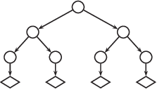
A useful geometric visualisation (which is, however, not essential for the proof) is obtained by placing these states at the vertices of an mm-ary tree (in this case of depth 33). We place |Ψ⟩|\Psi\rangle at the root, and the descendants of each vertex are the split states obtained by splitting. Thus every 33-tuple (α1,α2,α3)∈[m]3(\alpha_{1},\alpha_{2},\alpha_{3})\in[m]^{3} specifies a path with vertex labels (|Ψ⟩,|Ψα1⟩,|Ψα1​α2⟩,|Ψα1​α2​α3⟩)(|\Psi\rangle,|\Psi^{\alpha_{1}}\rangle,|\Psi^{\alpha_{1}\alpha_{2}}\rangle,|\Psi^{\alpha_{1}\alpha_{2}\alpha_{3}}\rangle) from the root to a leaf.

Let us combine inequalities (19)–(21) into

Hmin​(X4|E)ρ\displaystyle H_{\min}(X^{4}|E)_{\rho} ≲Hmin​(X1|X>1​E)ρα1+Hmin​(X2|X>2​E)ρα1​α2\displaystyle\lesssim H_{\min}(X_{1}|X_{>1}E)_{\rho^{\alpha_{1}}}+H_{\min}(X_{2}|X_{>2}E)_{\rho^{\alpha_{1}\alpha_{2}}}
+Hmin​(X3|X>3​E)ρα1​α2​α3+Hmin​(X4|E)ρα1​α2​α3for all ​α3=(α1,α2,α3)∈[m]3.\displaystyle\ \ \ +H_{\min}(X_{3}|X_{>3}E)_{\rho^{\alpha_{1}\alpha_{2}\alpha_{3}}}+H_{\min}(X_{4}|E)_{\rho^{\alpha_{1}\alpha_{2}\alpha_{3}}}\qquad\textrm{for all }\alpha^{3}=(\alpha_{1},\alpha_{2},\alpha_{3})\in[m]^{3}\ .

By attaching the entropies of interest to the edges of the mentioned tree, we can interpret this inequality as expressing the fact that the sum of the values of the edges along each path of the tree from the root to a leaf is lower bounded by Hmin​(X4|E)ρH_{\min}(X^{4}|E)_{\rho}.

The next things to consider are the sampling- and recombination step. Our aim is to show that the smooth entropy Hminε​(X𝒮|E)ρH_{\min}^{\varepsilon}(X_{\mathcal{S}}|E)_{\rho} is large (with high probability over the choice of the subset 𝒮⊂[4]\mathcal{S}\subset[4]). We follow the procedure outlined in the previous section. That is, we define the recombined state

|Ψ^⟩\displaystyle|\widehat{\Psi}\rangle =∑α3∈Γ⁡(λ,𝒮)|Ψα3⟩\displaystyle=\sum_{\alpha^{3}\in\Gamma(\lambda,\mathcal{S})}|\Psi^{\alpha^{3}}\rangle

where Γ⁡(λ,𝒮)\Gamma(\lambda,\mathcal{S}) is the set of paths α3∈[m]3\alpha^{3}\in[m]^{3} with the property that

δ1∈𝒮​Hmin​(X1|X>1​E)ρα1+δ2∈𝒮​Hmin​(X2|X>2​E)ρα1​α2\displaystyle\delta_{1\in\mathcal{S}}H_{\min}(X_{1}|X_{>1}E)_{\rho^{\alpha_{1}}}+\delta_{2\in\mathcal{S}}H_{\min}(X_{2}|X_{>2}E)_{\rho^{\alpha_{1}\alpha_{2}}}
+δ3∈𝒮​Hmin​(X3|X>3​E)ρα1​α2​α3+δ4∈𝒮​Hmin​(X4|E)ρα1​α2​α3\displaystyle\qquad+\delta_{3\in\mathcal{S}}H_{\min}(X_{3}|X_{>3}E)_{\rho^{\alpha_{1}\alpha_{2}\alpha_{3}}}+\delta_{4\in\mathcal{S}}H_{\min}(X_{4}|E)_{\rho^{\alpha_{1}\alpha_{2}\alpha_{3}}} ≥λ.\displaystyle\geq\lambda\ .

In other words, we restrict our attention to paths (and corresponding states) which (when restricted to 𝒮\mathcal{S}), have large entropy. We then need to show the following:

  1. (i)

    with high probability over the choice 𝒮\mathcal{S}, the state |Ψ^⟩|\widehat{\Psi}\rangle is close to |Ψ⟩|\Psi\rangle

  2. (ii)

    the entropy H​(X𝒮|E)ρ^H(X_{\mathcal{S}}|E)_{\hat{\rho}} is large.

The proof of (i) again involves a bound of the form

12​‖|Ψ⟩​⟨Ψ|−|Ψ^⟩​⟨Ψ^|‖≤1−ω⁡(Γ⁡(λ,𝒮)),\frac{1}{2}\big\||\Psi\rangle\langle\Psi|-|\widehat{\Psi}\rangle\langle\widehat{\Psi}|\big\|\leq\sqrt{1-\omega(\Gamma(\lambda,\mathcal{S}))}\ ,

where ω⁡(α3)=𝗍𝗋⁡|Ψα3⟩​⟨Ψα3|\omega(\alpha^{3})=\mathsf{tr}|\Psi^{\alpha^{3}}\rangle\langle\Psi^{\alpha^{3}}|, α3∈[m]3\alpha^{3}\in[m]^{3} is a (fixed) probability distribution on the leaves. We will show that a sampler has the following property, when applied to the situation described above (see Section 6.3): With high probability over the choice of 𝒮\mathcal{S}, the weight ω⁡(Γ⁡(λ,𝒮))\omega(\Gamma(\lambda,\mathcal{S})) is large. More generally, we show how the sampler-property extends from a single sequence of values to the case of a matrix of values (in our case corresponding to edges of a tree).

The proof of (ii) is done inductively using subadditivity, the recombination-chain-rule, and the recombination argument outlined above. For concreteness, suppose for example that 𝒮={2,4}\mathcal{S}=\{2,4\}. Then we have

Hmin​(X2|X>2​E)ρα1​α2+Hmin​(X4|E)ρα1​α2​α3≥λ\displaystyle H_{\min}(X_{2}|X_{>2}E)_{\rho^{\alpha_{1}\alpha_{2}}}+H_{\min}(X_{4}|E)_{\rho^{\alpha_{1}\alpha_{2}\alpha_{3}}}\geq\lambda\

for all α3=(α1,α2,α3)∈Γ⁡(λ,𝒮)⊂[m]3\alpha^{3}=(\alpha_{1},\alpha_{2},\alpha_{3})\in\Gamma(\lambda,\mathcal{S})\subset[m]^{3}. It is convenient to rephrase this as follows, writing α3=(α2,α3)\alpha^{3}=(\alpha^{2},\alpha_{3}). We then have for all α2∈[m]2\alpha^{2}\in[m]^{2}

Hmin​(X4|E)ρ(α2,α3)≥λ−Hmin​(X2|X>2​E)ρα2 for all ​α3​ with ​(α2,α3)∈Γ⁡(λ,𝒮).\displaystyle H_{\min}(X_{4}|E)_{\rho^{(\alpha^{2},\alpha_{3})}}\geq\lambda-H_{\min}(X_{2}|X_{>2}E)_{\rho^{\alpha^{2}}}\qquad\textrm{ for all }\alpha_{3}\textrm{ with }(\alpha^{2},\alpha_{3})\in\Gamma(\lambda,\mathcal{S})\ .

In particular, when we apply this to the (intermediate) partially recombined states

|Ψ^α2⟩=∑α3:(α2,α3)∈Γ⁡(λ,𝒮)|Ψ(α2,α3)⟩,\displaystyle|\widehat{\Psi}^{\alpha^{2}}\rangle=\sum_{\alpha_{3}:(\alpha^{2},\alpha_{3})\in\Gamma(\lambda,\mathcal{S})}|\Psi^{(\alpha^{2},\alpha_{3})}\rangle\ , (22)

we obtain

Hmin​(X4|E)ρ^α2≳λ−Hmin​(X2|X>2​E)ρα2 for all ​α2.\displaystyle H_{\min}(X_{4}|E)_{\widehat{\rho}^{\alpha^{2}}}\gtrsim\lambda-H_{\min}(X_{2}|X_{>2}E)_{\rho^{\alpha^{2}}}\qquad\textrm{ for all }\alpha^{2}\ .

We will also use the fact that the recombined states satisfy Hmin​(X2|X>2​E)ρ^α2≥Hmin​(X2|X>2​E)ρα2H_{\min}(X_{2}|X_{>2}E)_{\widehat{\rho}^{\alpha^{2}}}\geq H_{\min}(X_{2}|X_{>2}E)_{\rho^{\alpha^{2}}} (see Lemma 6.6(v)). Subadditivity gives Hmin​(X2|X4​E)ρ^α2≥Hmin​(X2|X>2​E)ρ^α2H_{\min}(X_{2}|X_{4}E)_{\widehat{\rho}^{\alpha^{2}}}\geq H_{\min}(X_{2}|X_{>2}E)_{\widehat{\rho}^{\alpha^{2}}} for all α2∈[m]\alpha^{2}\in[m]. With the previous two inequalities, we therefore get

Hmin​(X4|E)ρ^α2+Hmin​(X2|X4​E)ρ^α2≳λ.\displaystyle H_{\min}(X_{4}|E)_{\widehat{\rho}^{\alpha^{2}}}+H_{\min}(X_{2}|X_{4}E)_{\widehat{\rho}^{\alpha^{2}}}\gtrsim\lambda\ .

This in turn implies

Hmin​(X2​X4|E)ρ^α2≳λfor all ​α2∈[m]2\displaystyle H_{\min}(X_{2}X_{4}|E)_{\widehat{\rho}^{\alpha^{2}}}\gtrsim\lambda\qquad\textrm{for all }\alpha^{2}\in[m]^{2}

by the recombination-chain-rule. Because |Ψ^⟩|\widehat{\Psi}\rangle can be written as sum of the states (22), the recombination-procedure then gives

Hmin​(X2​X4|E)ρ^≳λ,\displaystyle H_{\min}(X_{2}X_{4}|E)_{\widehat{\rho}}\gtrsim\lambda\ ,

as claimed.

This line of argument can be followed more generally for a general subset 𝒮⊂[n]\mathcal{S}\subset[n]. We will need intermediate (partially) recombined states {|Ψ^αj⟩}αj∈[m]j,j∈[n]\{|\widehat{\Psi}^{\alpha^{j}}\rangle\}_{\alpha^{j}\in[m]^{j}},j\in[n]; these can again be thought of as being attached to the vertices of a tree. They are defined recursively, by recombining “good” states (i.e., those corresponding to prefixes of elements in Γ⁡(λ,𝒮)\Gamma(\lambda,\mathcal{S})). In other words, when recombining, we work our way up the tree (omitting “bad” states, i.e., those with small entropies.)

This concludes our sketch proof; it is now time to elaborate on the details.

5 Rules and tools for min-entropy

In this section, we set the ground for our result concerning samplers. In particular, we formally introduce the conditional min-entropy Hmin​(A|B)ρH_{\min}(A|B)_{\rho} in Section 5.2. This will be done via an intermediate quantity H​(A|B)ρσH(A|B)_{\frac{\rho}{\sigma}}. Most of our rules for min-entropy, the most basic of which are stated in Section 5.3, apply to these intermediate quantities; they will be our main object of study. In Section 5.4, we establish our central splitting-chain-rule.

5.1 Preliminaries

Throughout, we consider nonnegative operators acting on finite-dimensional Hilbert spaces (or systems) ℋA,ℋB,…\mathcal{H}_{A},\mathcal{H}_{B},\ldots and their tensor products. We use subscripts to indicate which systems an operator acts on. We also use subscripts when we trace out systems, but sometimes make use of superscripts to denote “tracing out everything but”, in the following sense: for a tripartite state ρA​B​C\rho_{ABC}, we write 𝗍𝗋B​C​(ρA​B​C)=𝗍𝗋A¯​(ρA​B​C)=ρA\mathsf{tr}_{BC}(\rho_{ABC})=\mathsf{tr}_{\overline{A}}(\rho_{ABC})=\rho_{A} for the reduced density operator on AA. As explained above, we sometimes abuse notation by omitting identities. For example, we will write operator inequalities such as

ρA​B≤σB,\displaystyle\rho_{AB}\leq\sigma_{B}\ ,

for a bipartite operator ρA​B\rho_{AB} and an operator σB\sigma_{B} on ℋB\mathcal{H}_{B}. By this inequality, we simply mean ρA​B≤𝗂𝖽A⊗σB\rho_{AB}\leq\mathsf{id}_{A}\otimes\sigma_{B} (which is defined by the condition that 𝗂𝖽A⊗σB−ρA​B\mathsf{id}_{A}\otimes\sigma_{B}-\rho_{AB} is a nonnegative operator). More generally, when writing operators on multipartite systems, we omit identities whenever a unique meaningful statement can be obtained by tensoring corresponding identities to the operators. To give an example, we will write expressions such as

QB​ρA​B​QB≤PD​ρA​B​C​D​PD,\displaystyle Q_{B}\rho_{AB}Q_{B}\leq P_{D}\rho_{ABCD}P_{D}\ ,

where the operators act on the spaces indicated by subscripts, instead of

(𝗂𝖽A⊗QB⊗𝗂𝖽C​D)​(ρA​B⊗𝗂𝖽C​D)​(𝗂𝖽A⊗QB⊗𝗂𝖽C​D)≤(𝗂𝖽A​B​C⊗PD)​ρA​B​C​D​(𝗂𝖽A​B​C⊗PD).\displaystyle(\mathsf{id}_{A}\otimes Q_{B}\otimes\mathsf{id}_{CD})(\rho_{AB}\otimes\mathsf{id}_{CD})(\mathsf{id}_{A}\otimes Q_{B}\otimes\mathsf{id}_{CD})\leq(\mathsf{id}_{ABC}\otimes P_{D})\rho_{ABCD}(\mathsf{id}_{ABC}\otimes P_{D})\ .

Basic properties of operator inequalities we need are their preservation under partial traces and the application of operators, i.e., the fact that ρA​B≤σA​B\rho_{AB}\leq\sigma_{AB} implies that

ρA≤σA\displaystyle\rho_{A}\leq\sigma_{A}\

and

TA​B​ρA​B​TA​B†≤TA​B​σA​B​TA​B†\displaystyle T_{AB}\rho_{AB}T^{\dagger}_{AB}\leq T_{AB}\sigma_{AB}T^{\dagger}_{AB}

for any operator TA​BT_{AB} on ℋA⊗ℋB\mathcal{H}_{A}\otimes\mathcal{H}_{B}.

For two operators ρA​B\rho_{AB} on ℋA⊗ℋB\mathcal{H}_{A}\otimes\mathcal{H}_{B} and σB\sigma_{B} on ℋB\mathcal{H}_{B} such that the support of ρB\rho_{B} is contained in the support of σB\sigma_{B}, the conditional operator ρA​BσB\frac{\rho_{AB}}{\sigma_{B}} is defined as1111 11 Note that for σB=ρB\sigma_{B}=\rho_{B}, definition (23) coincides with the conditional operator ρA|B=ρA​BρB\rho_{A|B}=\frac{\rho_{AB}}{\rho_{B}} discussed, e.g., in [Lei07].

ρA​BσB:=σB−1/2ρA​BσB−1/2.\displaystyle\frac{\rho_{AB}}{\sigma_{B}}:=\sigma_{B}^{-{{1}/{2}}}\rho_{AB}\sigma_{B}^{-{{1}/{2}}}\ . (23)

Here σB−1/2:=σB−1\sigma_{B}^{-{{1}/{2}}}:=\sqrt{\sigma_{B}^{-1}}, where σB−1\sigma_{B}^{-1} is the generalised inverse1212 12 The generalised inverse σ−1\sigma^{-1} of an operator σ\sigma is defined as the operator which has the same eigenspaces as σ\sigma with zero eigenvalue on the null eigenspace of σ\sigma and eigenvalues λ−1\lambda^{-1} on the eigenspace of σ\sigma corresponding to the eigenvalue λ>0\lambda>0. of σB\sigma_{B}. An important property of conditional operators is that

ρA​BσB=𝗍𝗋C​(ρA​B​CσB)\displaystyle\frac{\rho_{AB}}{\sigma_{B}}=\mathsf{tr}_{C}\bigl(\frac{\rho_{ABC}}{\sigma_{B}}\bigr)\ (24)

for any tripartite operator ρA​B​C\rho_{ABC}.

We will say that a bipartite operator ρA​E\rho_{AE} on ℋA⊗ℋE\mathcal{H}_{A}\otimes\mathcal{H}_{E} is classical on AA (relative to an orthonormal basis {|a⟩}a\{|a\rangle\}_{a} of ℋA\mathcal{H}_{A}) if it has the form ρA​E=∑a|a⟩​⟨a|A⊗ρEa\rho_{AE}=\sum_{a}|a\rangle\langle a|_{A}\otimes\rho^{a}_{E}. Clearly, if ρA​E\rho_{AE} is classical on AA relative to {|a⟩}a\{|a\rangle\}_{a}, then so is ρA​E′=OA​E​ρA​E​OA​E†\rho^{\prime}_{AE}=O_{AE}\rho_{AE}O_{AE}^{\dagger}, for any operator of the form OA​E=∑a|a⟩​⟨a|⊗OEaO_{AE}=\sum_{a}|a\rangle\langle a|\otimes O^{a}_{E}. It is easy to verify that this statement is still true when considering purifications and additional classical systems: If |ΨA​B​E​F⟩|\Psi_{ABEF}\rangle is such that the reduced density operator ρA​B​E\rho_{ABE} is classical on both AA and BB (relative to some orthonormal bases) then the same is true1313 13 This can be seen by decomposing the state as |ΨA​B​E​F⟩=∑a,b|a⟩​|b⟩​|φE​Fa,b⟩|\Psi_{ABEF}\rangle=\sum_{a,b}|a\rangle|b\rangle|\varphi^{a,b}_{EF}\rangle. Classicality of the state ρA​B​E\rho_{ABE} on AA and BB then implies that 𝗍𝗋F​(|φE​Fa,b⟩​⟨φE​Fa′,b′|)=0\mathsf{tr}_{F}(|\varphi^{a,b}_{EF}\rangle\langle\varphi^{a^{\prime},b^{\prime}}_{EF}|)=0 whenever (a,b)≠(a′,b′)(a,b)\neq(a^{\prime},b^{\prime}). The claim can then be deduced from the fact that 𝗍𝗋F​(OEa​|φE​Fa,b⟩​⟨φE​Fa′,b′|​(OEa′)†)=OEa​𝗍𝗋F​(|φE​Fa,b⟩​⟨φE​Fa′,b′|)​(OEa′)†\mathsf{tr}_{F}(O^{a}_{E}|\varphi^{a,b}_{EF}\rangle\langle\varphi^{a^{\prime},b^{\prime}}_{EF}|(O^{a^{\prime}}_{E})^{\dagger})=O^{a}_{E}\mathsf{tr}_{F}(|\varphi^{a,b}_{EF}\rangle\langle\varphi^{a^{\prime},b^{\prime}}_{EF}|)(O^{a^{\prime}}_{E})^{\dagger}. for the state OA​E​|ΨA​B​E​F⟩O_{AE}|\Psi_{ABEF}\rangle.

5.2 Definition of min-entropy

As already mentioned, every pair of operators ρA​B\rho_{AB} on ℋA⊗ℋB\mathcal{H}_{A}\otimes\mathcal{H}_{B} and σB\sigma_{B} on ℋB\mathcal{H}_{B} such that the support of ρB\rho_{B} is contained in the support of σB\sigma_{B} give rise to a conditional operator ρA​BσB\frac{\rho_{AB}}{\sigma_{B}}.1414 14 In the following, we will always assume that the support of ρB\rho_{B} is contained in the support of σB\sigma_{B}, such that the conditional operator is well defined. We define the quantity H​(A|B)ρσH(A|B)_{\frac{\rho}{\sigma}} as minus the logarithm1515 15 All logarithms log\log are binary; natural logarithms will be denoted by ln\ln. of the maximal eigenvalue of this conditional operator, that is

H​(A|B)ρσ:=−log⁡λmax​(ρA​BσB).\displaystyle H(A|B)_{\frac{\rho}{\sigma}}:=-\log\lambda_{\max}(\frac{\rho_{AB}}{\sigma_{B}})\ .

In some sense, this can be read as “the entropy of ρA\rho_{A} when it is conditioned on σB\sigma_{B}”; in the case where AA is classical, the operator σB\sigma_{B} is related to a measurement on ℋB\mathcal{H}_{B} (which is supposed to reproduce the value on AA, see [KSR07]).

Maximising this quantity over all nonnegative trace-one operators σB\sigma_{B} whose support contains the support of ρB\rho_{B} gives the min-entropy of AA given BB, defined as1616 16 In Section 2.6, the quantity Hmin​(A|B)ρH_{\min}(A|B)_{\rho} was introduced without explicit reference to the intermediate quantities H​(A|B)ρσH(A|B)_{\frac{\rho}{\sigma}}.

Hmin​(A|B)ρ:=supσBH​(A|B)ρσ.\displaystyle H_{\min}(A|B)_{\rho}:=\sup_{\sigma_{B}}H(A|B)_{\frac{\rho}{\sigma}}\ . (25)

This quantity has a simple operational interpretation, as will be shown in a forthcoming publication [KSR07]: it is equivalent to the maximal probability of guessing AA given BB, in the case where AA is classical.

While (25) is ultimately the quantity of interest, the intermediate quantities H​(A|B)ρσH(A|B)_{\frac{\rho}{\sigma}} are easier to manipulate, and satisfy various useful rules. As we will see below, most of these follow more or less directly from the alternative characterisation

H​(A|B)ρσ\displaystyle H(A|B)_{\frac{\rho}{\sigma}} :=−log⁡min⁡{λ:ρA​BσB≤λ⋅𝗂𝖽A​B}\displaystyle:=-\log\min\{\lambda\ :\ \frac{\rho_{AB}}{\sigma_{B}}\leq\lambda\cdot\mathsf{id}_{AB}\} (26)

in terms of a family of operator inequalities.

For consistency reasons, it is convenient to set

H​(A|B)ρ\displaystyle H(A|B)_{\rho} :=H​(A|B)ρρ\displaystyle:=H(A|B)_{\frac{\rho}{\rho}}
H​(∅|B)ρσ\displaystyle H(\emptyset|B)_{\frac{\rho}{\sigma}} :=−log⁡min⁡{λ:ρBσB≤λ⋅𝗂𝖽},\displaystyle:=-\log\min\{\lambda\ :\ \frac{\rho_{B}}{\sigma_{B}}\leq\lambda\cdot\mathsf{id}\}\ ,

where ρBσB=σB−1/2ρBσB−1/2\frac{\rho_{B}}{\sigma_{B}}=\sigma_{B}^{-{{1}/{2}}}\rho_{B}\sigma_{B}^{-{{1}/{2}}}. Note that the latter quantity is equal to H​(A|B)ρσH(A|B)_{\frac{\rho}{\sigma}} if the Hilbert space ℋA\mathcal{H}_{A} corresponding to system AA is trivial, i.e., ℋA≅ℂ\mathcal{H}_{A}\cong\mathbb{C}. We can think of the quantity H​(B)ρσH(B)_{\frac{\rho}{\sigma}} as a conditional entropy obtained by adjoining a trivial system to BB using the isomorphism ℋB≅ℋB⊗ℂ\mathcal{H}_{B}\cong\mathcal{H}_{B}\otimes\mathbb{C}. Informally, this corresponds to a situation where we condition “nothing” on σB\sigma_{B}; formally, it will turn out to be convenient to define H​(∅|B)ρσ:=H​(∅|B)ρσH(\emptyset|B)_{\frac{\rho}{\sigma}}:=H(\emptyset|B)_{\frac{\rho}{\sigma}}.

Finally, we will also (formally) encounter situations where ρA​B=0\rho_{AB}=0; in these cases, we formally set H​(A|B)ρ=∞H(A|B)_{\rho}=\infty, H​(A|B)ρσ=∞H(A|B)_{\frac{\rho}{\sigma}}=\infty, meaning that an arbitrarily large value can be assigned to these quantities in any identity where they appear.

For a parameter ε≥0\varepsilon\geq 0, the ε\varepsilon-smooth min-entropy of AA given BB is equal to (cf. [Ren05])

Hminε(A|B)ρ=supρ¯A​B:‖ρ¯A​B−ρA​B‖≤ε𝗍𝗋⁡(ρ¯A​B)≤1Hmin(A|B)ρ¯,\displaystyle H_{\min}^{\varepsilon}(A|B)_{\rho}=\sup_{\begin{subarray}{c}\bar{\rho}_{AB}:\|\bar{\rho}_{AB}-\rho_{AB}\|\leq\varepsilon\\ \mathsf{tr}(\bar{\rho}_{AB})\leq 1\end{subarray}}H_{\min}(A|B)_{\bar{\rho}}\ ,

where the supremum is over all nonnegative operators ρ¯A​B\bar{\rho}_{AB} with trace bounded by 11 in an ε\varepsilon-ball around ρA​B\rho_{AB}. (Here ‖A‖=𝗍𝗋​A†​A\|A\|=\mathsf{tr}\sqrt{A^{\dagger}A} is the L1L_{1}-norm.)

As already mentioned, the (smooth) entropy Hminε​(X|E)H_{\min}^{\varepsilon}(X|E) captures the number of secret bits extractable from XX with respect to an adversary holding EE. The following lemma justifies this operational interpretation.

Lemma 5.1.

Consider a state ρX​E\rho_{XE} where XX is classical. Let ρ𝒰{0,1}ℓ\rho_{\mathcal{U}_{\{0,1\}^{\ell}}} denote the completely mixed state on {0,1}ℓ\{0,1\}^{\ell}. Then

  1. (i)

    For any ℓ≤Hmin​(X|E)−2​log⁡1/ε\ell\leq H_{\min}(X|E)-2\log{{1}/{\varepsilon}}, there is a function f:𝒳×𝒳→{0,1}ℓf:\mathcal{X}\times\mathcal{X}\rightarrow\{0,1\}^{\ell} (independent of ρX​E\rho_{XE}) which extracts an ℓ\ell-bit string Z=f⁡(X,Y)Z=f(X,Y) from XX, such that ZZ is ε\varepsilon-close to uniform and independent of (E,Y)(E,Y), where YY is a uniform and independent seed. In formulae, we have

    12​‖ρf⁡(X,Y)​Y​E−ρ𝒰{0,1}ℓ⊗ρY⊗ρE‖≤ε.\displaystyle\frac{1}{2}\|\rho_{f(X,Y)YE}-\rho_{\mathcal{U}_{\{0,1\}^{\ell}}}\otimes\rho_{Y}\otimes\rho_{E}\|\leq\varepsilon\ .
  2. (ii)

    For any function f:𝒳→{0,1}ℓf:\mathcal{X}\rightarrow\{0,1\}^{\ell} and ε≥0\varepsilon\geq 0, the inequality

    12​‖ρf⁡(X)​E−ρ𝒰{0,1}ℓ⊗ρE‖≤ε\frac{1}{2}\bigl\|\rho_{f(X)E}-\rho_{\mathcal{U}_{\{0,1\}^{\ell}}}\otimes\rho_{E}\bigr\|\leq\varepsilon

    implies

    Hmin2​ε​(X|E)ρ≥ℓ.H_{\min}^{2\varepsilon}(X|E)_{\rho}\geq\ell\ .
Proof.

Statement (i) is a reformulation of the fact that the two-universal hashing construction is a quantum extractor, as shown by Renner [Ren05].

For the proof of (ii), let ρ¯S​E:=ρ𝒰{0,1}ℓ⊗ρE\bar{\rho}_{SE}:=\rho_{\mathcal{U}_{\{0,1\}^{\ell}}}\otimes\rho_{E}. Then, obviously

Hmin​(S|E)ρ¯≥H​(S|E)ρ¯ρ¯=ℓ.H_{\min}(S|E)_{\bar{\rho}}\geq H(S|E)_{\frac{\bar{\rho}}{\bar{\rho}}}=\ell\ .

Because 12​‖ρ¯S​E−ρf⁡(X)​E‖≤ε\frac{1}{2}\|\bar{\rho}_{SE}-\rho_{f(X)E}\|\leq\varepsilon, this implies

Hmin2​ε​(f⁡(X)|E)ρ≥Hmin​(S|E)ρ¯≥ℓ.H_{\min}^{2\varepsilon}(f(X)|E)_{\rho}\geq H_{\min}(S|E)_{\bar{\rho}}\geq\ell\ .

Since the min-entropy can only decrease when applying a function (see [Ren05]), we conclude that

Hmin2​ε​(X|E)ρ≥Hmin2​ε​(f⁡(X)|E)ρ≥ℓ,H_{\min}^{2\varepsilon}(X|E)_{\rho}\geq H_{\min}^{2\varepsilon}(f(X)|E)_{\rho}\geq\ell\ ,

as desired. ∎

5.3 Some basic rules and properties

We now summarise a few basic rules for the quantities H​(A|B)ρσH(A|B)_{\frac{\rho}{\sigma}} which directly follow from (26) using standard properties of operator inequalities, as described in Section 5.1.

Lemma 5.2 (Properties of min-entropy).

The min-entropy satisfies the following.

  1. (i)

    (Positivity for classical systems) Let ρA​B=∑a|a⟩​⟨a|⊗ρBa\rho_{AB}=\sum_{a}|a\rangle\langle a|\otimes\rho_{B}^{a} be classical on AA. Then H​(A|B)ρ≥0H(A|B)_{\rho}\geq 0.

  2. (ii)

    (Dimension bound) For any ρA​B\rho_{AB} and σB\sigma_{B} with σB≤ρB\sigma_{B}\leq\rho_{B}, we have H​(A|B)ρσ≤H0​(A)H(A|B)_{\frac{\rho}{\sigma}}\leq H_{0}(A), where H0(A)=logdimℋAH_{0}(A)=\log\dim\mathcal{H}_{A}. In particular, H​(A|B)ρ≤H0​(A)H(A|B)_{\rho}\leq H_{0}(A). More generally H​(B|C)ρσ≥H​(A​B|C)ρσ−H0​(A)H(B|C)_{\frac{\rho}{\sigma}}\geq H(AB|C)_{\frac{\rho}{\sigma}}-H_{0}(A) for any ρA​B​C\rho_{ABC} and σC\sigma_{C}.

  3. (iii)

    (Subadditivity) H​(A|B)ρσ≥H​(A|B​C)ρσH(A|B)_{\frac{\rho}{\sigma}}\geq H(A|BC)_{\frac{\rho}{\sigma}} for any ρA​B​C\rho_{ABC} and σB​C\sigma_{BC}.

  4. (iv)

    (Recombination-chain-rule) H​(A​B|C)ρσ≥H​(A|B​C)ρ+H​(B|C)ρσH(AB|C)_{\frac{\rho}{\sigma}}\geq H(A|BC)_{\rho}+H(B|C)_{\frac{\rho}{\sigma}} for any ρA​B​C\rho_{ABC} and σC\sigma_{C}.

Proof.

(i) directly follows from |a⟩​⟨a|⊗ρBa≤ρB|a\rangle\langle a|\otimes\rho_{B}^{a}\leq\rho_{B} for all aa.

For the proof of the first part of (ii), we simply take the trace on both sides of the inequality ρA​B≤2−H​(A|B)ρσ​σB\rho_{AB}\leq 2^{-H(A|B)_{\frac{\rho}{\sigma}}}\sigma_{B} to get 𝗍𝗋⁡(ρA​B)≤2H0​(A)−H​(A|B)ρσ​𝗍𝗋​(σB)\mathsf{tr}(\rho_{AB})\leq 2^{H_{0}(A)-H(A|B)_{\frac{\rho}{\sigma}}}\mathsf{tr}(\sigma_{B}), which gives the claim because 𝗍𝗋⁡(σB)≤𝗍𝗋⁡(ρB)=𝗍𝗋⁡(ρA​B)\mathsf{tr}(\sigma_{B})\leq\mathsf{tr}(\rho_{B})=\mathsf{tr}(\rho_{AB}). For the proof of the second part of (ii), observe that we have ρA​B​C≤2−H​(A​B|C)ρσ​σC\rho_{ABC}\leq 2^{-H(AB|C)_{\frac{\rho}{\sigma}}}\sigma_{C} by definition. Tracing out the system AA gives

ρB​C≤2−H​(A​B|C)ρσ+H0​(A)​σC.\displaystyle\rho_{BC}\leq 2^{-H(AB|C)_{\frac{\rho}{\sigma}}+H_{0}(A)}\sigma_{C}\ .

The claim (ii) then follows from the definition of H​(B|C)ρσH(B|C)_{\frac{\rho}{\sigma}}.

Similarly, (iii) directly follows by tracing out CC from the inequality

ρA​B​C≤2−H​(A|B​C)ρσ​σB​C.\rho_{ABC}\leq 2^{-H(A|BC)_{\frac{\rho}{\sigma}}}\sigma_{BC}\ .

For the proof of (iv), observe that

ρA​B​C\displaystyle\rho_{ABC} ≤2−H​(A|B​C)ρ​ρB​C≤2−H​(A|B​C)ρ−H​(B|C)ρσ​σC.\displaystyle\leq 2^{-H(A|BC)_{\rho}}\rho_{BC}\leq 2^{-H(A|BC)_{\rho}-H(B|C)_{\frac{\rho}{\sigma}}}\sigma_{C}\ .

The claim follows from the definition of H​(A​B|C)ρσH(AB|C)_{\frac{\rho}{\sigma}}. ∎

We point out that (ii) and (iii) directly translate into the statements

Hmin​(B|C)ρ\displaystyle H_{\min}(B|C)_{\rho} ≥Hmin​(A​B|C)ρ−H0​(A)\displaystyle\geq H_{\min}(AB|C)_{\rho}-H_{0}(A)
Hmin​(A|B)ρ\displaystyle H_{\min}(A|B)_{\rho} ≥Hmin​(A|B​C)ρ\displaystyle\geq H_{\min}(A|BC)_{\rho}

for the min-entropy. An analogous statement cannot be made for the recombination-chain-rule (iv), and we will have to retain the dependence on σC\sigma_{C} in our arguments.

Having established subadditivity and a recombination-chain-rule, we will address the problem of finding a converse splitting-chain-rule in the next section. Before doing so, however, we will mention another property of the min-entropy which will be important for our purposes. This is the fact the entropy of a state |Ψ′⟩=Q​|Ψ⟩|\Psi^{\prime}\rangle=Q|\Psi\rangle obtained by applying a projection to a state |Ψ⟩|\Psi\rangle is lower bounded by the entropy of the original state. We will later see that this allows us to retain information about the entropy when going from a state to its split descendants.

Note that this statement is not generally true, but depends crucially on where the projection acts.

Lemma 5.3 (Monotony under projections).

Let |ΨA​B​C⟩|\Psi_{ABC}\rangle be a pure state, let QCQ_{C} be an operator on CC and let |ΨA​B​C′⟩=QC​|ΨA​B​C⟩|\Psi_{ABC}^{\prime}\rangle=Q_{C}|\Psi_{ABC}\rangle. Let ρA​B​C\rho_{ABC} and ρA​B​C′\rho^{\prime}_{ABC} be the corresponding density operators. Then

H​(A|B​C)ρ′≥H​(A|B​C)ρ.\displaystyle H(A|BC)_{\rho^{\prime}}\geq H(A|BC)_{\rho}\ .

Furthermore, if QCQ_{C} is a projector, then

H​(A|B)ρ′σ≥H​(A|B)ρσ and H​(∅|B)ρ′σ≥H​(∅|B)ρσ\displaystyle H(A|B)_{\frac{\rho^{\prime}}{\sigma}}\geq H(A|B)_{\frac{\rho}{\sigma}}\qquad\textrm{ and }\qquad H(\emptyset|B)_{\frac{\rho^{\prime}}{\sigma}}\geq H(\emptyset|B)_{\frac{\rho}{\sigma}}

for arbitrary σ=σC\sigma=\sigma_{C}.

Proof.

To prove the first inequality, let QCQ_{C} be arbitrary. Applying QCQ_{C} from the left and QC†Q_{C}^{\dagger} from the right to both sides of the inequality

ρA​B​C≤2−H​(A|B​C)ρ​ρB​C\displaystyle\rho_{ABC}\leq 2^{-H(A|BC)_{\rho}}\rho_{BC}\

gives

ρA​B​C′≤2−H​(A|B​C)ρ​ρB​C′\displaystyle\rho^{\prime}_{ABC}\leq 2^{-H(A|BC)_{\rho}}\rho^{\prime}_{BC}

by definition of |ΨA​B​C′⟩|\Psi^{\prime}_{ABC}\rangle and the properties of the partial trace. This proves the first inequality.

Let now QCQ_{C} be a projector, and let |φA​B⟩∈A​B|\varphi_{AB}\rangle\in AB be arbitrary. Then

𝗍𝗋⁡(|φA​B⟩​⟨φA​B|​ρA​B′)\displaystyle\mathsf{tr}(|\varphi_{AB}\rangle\langle\varphi_{AB}|\rho^{\prime}_{AB}) =𝗍𝗋⁡((|φA​B⟩​⟨φA​B|⊗𝗂𝖽C)​ρA​B​C′)\displaystyle=\mathsf{tr}\left((|\varphi_{AB}\rangle\langle\varphi_{AB}|\otimes\mathsf{id}_{C})\rho^{\prime}_{ABC}\right)
=𝗍𝗋⁡((|φA​B⟩​⟨φA​B|⊗QC)​ρA​B​C)\displaystyle=\mathsf{tr}\left((|\varphi_{AB}\rangle\langle\varphi_{AB}|\otimes Q_{C})\rho_{ABC}\right)\

by the cyclicity of the trace and the fact that QCQ_{C} is a projector. In particular, with QC⊥=𝗂𝖽C−QCQ_{C}^{\bot}=\mathsf{id}_{C}-Q_{C} denoting the projector onto the orthogonal complement of the image of QCQ_{C}, we have

𝗍𝗋⁡(|φA​B⟩​⟨φA​B|​(ρA​B−ρA​B′))\displaystyle\mathsf{tr}\left(|\varphi_{AB}\rangle\langle\varphi_{AB}|(\rho_{AB}-\rho^{\prime}_{AB})\right) =𝗍𝗋⁡((|φA​B⟩​⟨φA​B|⊗QC⊥)​ρA​B​C)≥0.\displaystyle=\mathsf{tr}\left((|\varphi_{AB}\rangle\langle\varphi_{AB}|\otimes Q_{C}^{\bot})\rho_{ABC}\right)\geq 0\ .

We conclude that ρA​B′≤ρA​B\rho_{AB}^{\prime}\leq\rho_{AB}. In particular,

ρA​B′≤ρA​B≤2−H​(A|B)ρσ​σB and ρB′≤ρB≤2−H​(∅|B)ρσ​σB\displaystyle\rho_{AB}^{\prime}\leq\rho_{AB}\leq 2^{-H(A|B)_{\frac{\rho}{\sigma}}}\sigma_{B}\qquad\textrm{ and }\qquad\rho^{\prime}_{B}\leq\rho_{B}\leq 2^{-H(\emptyset|B)_{\frac{\rho}{\sigma}}}\sigma_{B}

which implies the claim. ∎

5.4 Entropy-splitting: A splitting-chain-rule for min-entropy

To introduce our splitting-chain-rule, we proceed in two steps: In Section 5.4.1, we show a simplified version which does not restrict the number of states the original state is split into. As this is irrelevant for the remainder of our proof, this section can be skipped; however, it nicely illustrates the relevant features. The case of interest, where we split a given state into a fixed number mm of states, can be seen as a coarse-graining of the former. It will be the topic of Section 5.4.2.

5.4.1 A warm-up

The chain-rule we will prove in this section concerns a tripartite state ρA​B​C\rho_{ABC} with purification ρA​B​C​D=|ΨA​B​C​D⟩​⟨ΨA​B​C​D|\rho_{ABCD}=|\Psi_{ABCD}\rangle\langle\Psi_{ABCD}| and an operator σC\sigma_{C}. We will show that we can split |ΨA​B​C​D⟩|\Psi_{ABCD}\rangle into a sum of states {|ΨA​B​C​Dα⟩}α\{|\Psi^{\alpha}_{ABCD}\rangle\}_{\alpha} as in (16), in a way that

H​(A|B​C)ρα+H​(B|C)ρασ≥H​(A​B|C)ρσ for all ​α,\displaystyle H(A|BC)_{\rho^{\alpha}}+H(B|C)_{\frac{\rho^{\alpha}}{\sigma}}\geq H(AB|C)_{\frac{\rho}{\sigma}}\qquad\textrm{ for all }\alpha\ , (27)

where ρA​B​C​Dα=|ΨA​B​C​Dα⟩​⟨ΨA​B​C​Dα|\rho^{\alpha}_{ABCD}=|\Psi^{\alpha}_{ABCD}\rangle\langle\Psi^{\alpha}_{ABCD}|. Note that by taking the supremum over σB\sigma_{B}, we immediately obtain the inequality

Hmin​(A|B​C)ρα+Hmin​(B|C)ρα≥Hmin​(A​B|C)ρ for all ​α\displaystyle H_{\min}(A|BC)_{\rho^{\alpha}}+H_{\min}(B|C)_{\rho^{\alpha}}\geq H_{\min}(AB|C)_{\rho}\qquad\textrm{ for all }\alpha\

from (27). However, (27) makes a stronger assertion, and we will generally deal with statements of this form.

For the proof of (27), consider the eigendecomposition

ρB​CσC=∑αα​PB​Cα\displaystyle\frac{\rho_{BC}}{\sigma_{C}}=\sum_{\alpha}\alpha P^{\alpha}_{BC}\

of the conditional operator, where PB​CαP^{\alpha}_{BC} is the projector onto the eigenspace corresponding to the eigenvalue α\alpha.

We will use the operators PB​CαP^{\alpha}_{BC} to define our split states, which will be labeled by the spectrum of ρB​CσC\frac{\rho_{BC}}{\sigma_{C}}. Clearly, if we apply PB​CαP^{\alpha}_{BC} on both sides of the operator ρB​CσC\frac{\rho_{BC}}{\sigma_{C}}, we end up with an operator which has a single non-zero eigenvalue α\alpha. While Pα​ρB​CσC​PαP^{\alpha}\frac{\rho_{BC}}{\sigma_{C}}P^{\alpha} thus has a very simple form, it is very different in nature from the original “unconditional” operator ρB​C\rho_{BC}. Intuitively, it therefore makes sense to multiply by σC\sigma_{C}. The appropriate definition of |ΨA​B​C​Dα⟩|\Psi^{\alpha}_{ABCD}\rangle turns out to be just the result of this, i.e., we can define1717 17 As above, we assume that the support of σC\sigma_{C} contains the support of ρC\rho_{C}, hence, σC\sigma_{C} is invertible on the relevant subspace.

|ΨA​B​C​Dα⟩=σC1/2PB​CασC−1/2|ΨA​B​C​D⟩.\displaystyle|\Psi^{\alpha}_{ABCD}\rangle=\sigma_{C}^{{{1}/{2}}}P^{\alpha}_{BC}\sigma_{C}^{-{{1}/{2}}}|\Psi_{ABCD}\rangle\ .

It is easy to check that these states decompose |ΨA​B​C​D⟩|\Psi_{ABCD}\rangle as in (16). They also satisfy (27), as we will show now. First observe that ρB​Cα=σC1/2​PB​Cα​ρB​CσC​PB​Cα​σC1/2\rho^{\alpha}_{BC}=\sigma_{C}^{{{1}/{2}}}P^{\alpha}_{BC}\frac{\rho_{BC}}{\sigma_{C}}P^{\alpha}_{BC}\sigma_{C}^{{{1}/{2}}} by their very definition, and thus

ρB​Cα=α⋅σC1/2​PB​Cα​σC1/2.\displaystyle\rho^{\alpha}_{BC}=\alpha\cdot\sigma_{C}^{{{1}/{2}}}P^{\alpha}_{BC}\sigma_{C}^{{{1}/{2}}}\ .

In particular, we have

ρB​CασC=α​PB​Cα,\displaystyle\frac{\rho^{\alpha}_{BC}}{\sigma_{C}}=\alpha P^{\alpha}_{BC}\ , (28)

which implies that

Hmin​(B|C)ρασ=−log⁡α.\displaystyle H_{\min}(B|C)_{\frac{\rho^{\alpha}}{\sigma}}=-\log\alpha\ . (29)

Combining (28) and (29) gives the statement

PB​Cα≤2Hmin​(B|C)ρασ​ρB​CασC.\displaystyle P^{\alpha}_{BC}\leq 2^{H_{\min}(B|C)_{\frac{\rho^{\alpha}}{\sigma}}}\frac{\rho^{\alpha}_{BC}}{\sigma_{C}}\ . (30)

By definition of the quantity H​(A​B|C)ρσH(AB|C)_{\frac{\rho}{\sigma}}, we also have ρA​B​CσC≤2−H​(A​B|C)ρσ\frac{\rho_{ABC}}{\sigma_{C}}\leq 2^{-H(AB|C)_{\frac{\rho}{\sigma}}}. Applying the projector PB​CαP^{\alpha}_{BC} on both sides of this inequality leads to

PB​Cα​ρA​B​CσC​PB​Cα≤2−H​(A​B|C)ρσ​PB​Cα≤2Hmin​(B|C)ρασ−H​(A​B|C)ρσ​ρB​CασC.\displaystyle P^{\alpha}_{BC}\frac{\rho_{ABC}}{\sigma_{C}}P^{\alpha}_{BC}\leq 2^{-H(AB|C)_{\frac{\rho}{\sigma}}}P^{\alpha}_{BC}\leq 2^{H_{\min}(B|C)_{\frac{\rho^{\alpha}}{\sigma}}-H(AB|C)_{\frac{\rho}{\sigma}}}\frac{\rho^{\alpha}_{BC}}{\sigma_{C}}\ .

Multiplying this inequality from both sides by σC1/2\sigma_{C}^{{{1}/{2}}} immediately gives the desired statement (27), since ρA​B​Cα=σC1/2​PB​Cα​ρA​B​CσC​PB​Cα​σC1/2\rho^{\alpha}_{ABC}=\sigma_{C}^{{{1}/{2}}}P^{\alpha}_{BC}\frac{\rho_{ABC}}{\sigma_{C}}P^{\alpha}_{BC}\sigma_{C}^{{{1}/{2}}}.

This concludes the proof of our simplified statement, where a state |ΨA​B​C​D⟩|\Psi_{ABCD}\rangle is split into a family {|ΨA​B​C​Dα⟩}α\{|\Psi^{\alpha}_{ABCD}\rangle\}_{\alpha}, each of which obeys the splitting-chain-rule inequality (27). The number of states is determined by the number of different eigenvalues of the operator ρB​CσC\frac{\rho_{BC}}{\sigma_{C}}; indeed, each state |ΨA​B​C​Dα⟩|\Psi^{\alpha}_{ABCD}\rangle corresponds to an eigenvalue α\alpha.

Before continuing, let us show the following useful properties of the states {|ΨA​B​C​Dα⟩}α\{|\Psi^{\alpha}_{ABCD}\rangle\}_{\alpha}: They are mutually orthogonal, and each state |ΨA​B​C​Dα⟩=QA​Dα​|Ψ⟩|\Psi^{\alpha}_{ABCD}\rangle=Q^{\alpha}_{AD}|\Psi\rangle is the result of applying a projection QA​DαQ^{\alpha}_{AD} (which acts non-trivially only on AA and DD) to |ΨA​B​C​D⟩|\Psi_{ABCD}\rangle. This statement is the result of using the complementarity property that is inherent in quantum states.

First observe that σC−1/2|ΨA​B​C​D⟩\sigma_{C}^{-{{1}/{2}}}|\Psi_{ABCD}\rangle is a purification of the conditional operator ρB​CσC\frac{\rho_{BC}}{\sigma_{C}}. Using the Schmidt-decomposition, we can write

σC−1/2|ΨA​B​C​D⟩=∑αα|α⟩A​D|α⟩B​C,\displaystyle\sigma_{C}^{-{{1}/{2}}}|\Psi_{ABCD}\rangle=\sum_{\alpha}\sqrt{\alpha}|\alpha\rangle_{AD}|\alpha\rangle_{BC}\ ,

where {|α⟩A​D}\{|\alpha\rangle_{AD}\} and {|α⟩B​C}\{|\alpha\rangle_{BC}\} are eigenvectors with eigenvalue α\alpha of ρA​DσC\frac{\rho_{AD}}{\sigma_{C}} and ρB​CσC\frac{\rho_{BC}}{\sigma_{C}}, respectively (slightly abusing notation, we omit multiplicities). We can define QA​DαQ^{\alpha}_{AD} as the projector onto the eigenspace of ρA​DσC\frac{\rho_{AD}}{\sigma_{C}} corresponding to the eigenvalue α\alpha. We then clearly have

PB​CασC−1/2|ΨA​B​C​D⟩=QA​DασC−1/2|ΨA​B​C​D⟩\displaystyle P^{\alpha}_{BC}\sigma_{C}^{-{{1}/{2}}}|\Psi_{ABCD}\rangle=Q^{\alpha}_{AD}\sigma_{C}^{-{{1}/{2}}}|\Psi_{ABCD}\rangle

for every α\alpha. Since σC1/2\sigma_{C}^{{{1}/{2}}} and QA​DαQ^{\alpha}_{AD} act on different systems, they commute, and we obtain

|ΨA​B​C​Dα⟩=σC1/2QA​DασC−1/2|ΨA​B​C​D⟩=QA​Dα|ΨA​B​C​D⟩,\displaystyle|\Psi^{\alpha}_{ABCD}\rangle=\sigma_{C}^{{{1}/{2}}}Q^{\alpha}_{AD}\sigma_{C}^{-{{1}/{2}}}|\Psi_{ABCD}\rangle=Q^{\alpha}_{AD}|\Psi_{ABCD}\rangle\ ,

as claimed. The orthogonality of these states is now immediate.

5.4.2 Splitting into a fixed number of states

In this section, we show that the construction discussed in Section 5.4.1 can be adapted to yield a fixed number mm of states. This is quite straightforward: We simply divide the spectrum of the conditional operator ρB​CσC\frac{\rho_{BC}}{\sigma_{C}} into mm different intervals ]μα−1,μα]]\mu_{\alpha-1},\mu_{\alpha}], for α∈[m]\alpha\in[m]. Instead of projecting onto the eigenspace corresponding to a single eigenvalue, we use projectors PB​CαP^{\alpha}_{BC} onto the direct sum of eigenspaces associated with eigenvalues in the corresponding interval.

Lemma 5.4 (Entropy splitting).

Let ρA​B​C​D=|ΨA​B​C​D⟩​⟨ΨA​B​C​D|\rho_{ABCD}=|\Psi_{ABCD}\rangle\langle\Psi_{ABCD}| be a pure state and let σC\sigma_{C} be a nonnegative operator. Let h0≤h1≤⋯≤hmh_{0}\leq h_{1}\leq\cdots\leq h_{m} be an (m+1)(m+1)-tuple of monotonically increasing real values with minimum and maximum given by

h0\displaystyle h_{0} :=H​(B|C)ρσ\displaystyle:=H(B|C)_{\frac{\rho}{\sigma}}
hm\displaystyle h_{m} :=H​(A​B|C)ρσ−H​(A|B​C)ρ.\displaystyle:=H(AB|C)_{\frac{\rho}{\sigma}}-H(A|BC)_{\rho}\ .

Then there are mutually orthogonal projectors {QA​Dα}α∈[m]\{Q^{\alpha}_{AD}\}_{\alpha\in[m]} with the property that

H​(A|B​C)ρα\displaystyle H(A|BC)_{\rho^{\alpha}} ≥H​(A​B|C)ρσ−hα\displaystyle\geq H(AB|C)_{\frac{\rho}{\sigma}}-h_{\alpha} (31)
H​(B|C)ρασ\displaystyle H(B|C)_{\frac{\rho^{\alpha}}{\sigma}} ≥hα−1\displaystyle\geq h_{\alpha-1} (32)

where ρA​B​C​Dα=|ΨA​B​C​Dα⟩​⟨ΨA​B​C​Dα|\rho^{\alpha}_{ABCD}=|\Psi^{\alpha}_{ABCD}\rangle\langle\Psi^{\alpha}_{ABCD}| is defined as

|ΨA​B​C​Dα⟩:=QA​Dα​|ΨA​B​C​D⟩.\displaystyle|\Psi_{ABCD}^{\alpha}\rangle:=Q^{\alpha}_{AD}|\Psi_{ABCD}\rangle\ . (33)

An alternative expression for these states is

|ΨA​B​C​Dα⟩:=σC1/2PB​CασC−1/2|ΨA​B​C​D⟩,\displaystyle|\Psi_{ABCD}^{\alpha}\rangle:=\sigma_{C}^{{{1}/{2}}}P^{\alpha}_{BC}\sigma_{C}^{-{{1}/{2}}}|\Psi_{ABCD}\rangle\ , (34)

where {PB​Cα}α∈[m]\{P^{\alpha}_{BC}\}_{\alpha\in[m]} are mutually orthogonal projectors. They satisfy

∑α∈[m]|Ψα⟩=|Ψ⟩\displaystyle\sum_{\alpha\in[m]}|\Psi^{\alpha}\rangle=|\Psi\rangle (35)

Note that, according to the chain rule (Lemma 5.2 (iv)), h0≤hmh_{0}\leq h_{m}, i.e., there always exists a tuple of reals as defined in the lemma.

Proof.

The proof of this statement is almost identical to the proof given in Section 5.4.1, but given here for completeness. For any α∈[m−1]\alpha\in[m-1], define μα:=2−hα\mu_{\alpha}:=2^{-h_{\alpha}}, and let μ0:=∞\mu_{0}:=\infty, μm:=−∞\mu_{m}:=-\infty. Note that (μα)α=0m(\mu_{\alpha})_{\alpha=0}^{m} is a monotonically decreasing sequence of values.

Consider the Schmidt-decomposition

σC−1/2|ΨA​B​C​D⟩=∑λλ|λ⟩B​C|λ⟩A​D\displaystyle\sigma_{C}^{-{{1}/{2}}}|\Psi_{ABCD}\rangle=\sum_{\lambda}\sqrt{\lambda}|\lambda\rangle_{BC}|\lambda\rangle_{AD}\ (36)

of the “conditional” state σC−1/2|ΨA​B​C​D⟩\sigma_{C}^{-{{1}/{2}}}|\Psi_{ABCD}\rangle (the sum may include multiplicities). For every α∈[m]\alpha\in[m], we define the projectors PB​CαP^{\alpha}_{BC} and QA​DαQ^{\alpha}_{AD} as

PB​Cα\displaystyle P^{\alpha}_{BC} =∑λ∈]μα,μα−1]|λ⟩⟨λ|B​C\displaystyle=\sum_{\lambda\in]\mu_{\alpha},\mu_{\alpha-1}]}|\lambda\rangle\langle\lambda|_{BC}
QA​Dα\displaystyle Q^{\alpha}_{AD} =∑λ∈]μα,μα−1]|λ⟩⟨λ|A​D.\displaystyle=\sum_{\lambda\in]\mu_{\alpha},\mu_{\alpha-1}]}|\lambda\rangle\langle\lambda|_{AD}\ .

By definition, these operators satisfy (33) and (34). Moreover, using the fact that QA​DαQ^{\alpha}_{AD} commutes with σC−1/2\sigma_{C}^{-{{1}/{2}}}, we conclude that (33) and (34) define the same state |ΨA​B​C​Dα⟩|\Psi^{\alpha}_{ABCD}\rangle.

Since PB​CαP^{\alpha}_{BC} is the projector onto the eigenspaces of ρB​CσC\frac{\rho_{BC}}{\sigma_{C}} which belong to the eigenvalues in ]μα,μα−1]]\mu_{\alpha},\mu_{\alpha-1}] for every α∈[m]\alpha\in[m], we have

μα​PB​Cα≤PB​Cα​ρB​CσC​PB​Cα≤μα−1​PB​Cα.\displaystyle\mu_{\alpha}P^{\alpha}_{BC}\leq P^{\alpha}_{BC}\frac{\rho_{BC}}{\sigma_{C}}P^{\alpha}_{BC}\leq\mu_{\alpha-1}P^{\alpha}_{BC}\ . (37)

We show that

PB​Cα​ρB​CσC​PB​Cα≤2−hα−1​PB​Cαfor all ​α∈[m].\displaystyle P^{\alpha}_{BC}\frac{\rho_{BC}}{\sigma_{C}}P^{\alpha}_{BC}\leq 2^{-h_{\alpha-1}}P^{\alpha}_{BC}\qquad\textrm{for all }\alpha\in[m]\ . (38)

This follows directly from (37) for α≥2\alpha\geq 2 since 2−hα−1=μα−12^{-h_{\alpha-1}}=\mu_{\alpha-1}; for α=1\alpha=1, it is a consequence of the fact that the eigenvalues of ρB​CσC\frac{\rho_{BC}}{\sigma_{C}} are upper bounded by 2−h02^{-h_{0}} by definition of h0h_{0}.

Claim (32) now directly follows from (38) and the fact that ρB​CασC=PB​Cα​ρB​CσC​PB​Cα\frac{\rho^{\alpha}_{BC}}{\sigma_{C}}=P^{\alpha}_{BC}\frac{\rho_{BC}}{\sigma_{C}}P^{\alpha}_{BC}.

Next we show that

PB​Cα​ρA​B​CσC​PB​Cα≤2−H​(A​B|C)ρσ+hα​PB​Cα​ρB​CσC​PB​Cα for all ​α∈[m].\displaystyle P^{\alpha}_{BC}\frac{\rho_{ABC}}{\sigma_{C}}P^{\alpha}_{BC}\leq 2^{-H(AB|C)_{\frac{\rho}{\sigma}}+h_{\alpha}}P^{\alpha}_{BC}\frac{\rho_{BC}}{\sigma_{C}}P^{\alpha}_{BC}\qquad\textrm{ for all }\alpha\in[m]\ . (39)

We distinguish two cases: For α=m\alpha=m, identity (39) is equivalent to

PB​Cα​ρA​B​CσC​PB​Cα≤2−H​(A|B​C)ρ​PB​Cα​ρB​CσC​PB​Cα\displaystyle P^{\alpha}_{BC}\frac{\rho_{ABC}}{\sigma_{C}}P^{\alpha}_{BC}\leq 2^{-H(A|BC)_{\rho}}P^{\alpha}_{BC}\frac{\rho_{BC}}{\sigma_{C}}P^{\alpha}_{BC}

because of the definition of hmh_{m}. But this directly follows from ρA​B​C≤2−H​(A|B​C)ρ​ρB​C\rho_{ABC}\leq 2^{-H(A|BC)_{\rho}}\rho_{BC} by multiplication from both sides with PαB​CσC−1/2P^{\alpha}_{BC}\sigma_{C}^{{-{{1}/{2}}}} and its adjoint.

For 1≤α<m1\leq\alpha<m, we use the fact that the first inequality of (37) is equivalent to

2−hα​PB​Cα≤PB​Cα​ρB​CσC​PB​Cα\displaystyle 2^{-h_{\alpha}}P^{\alpha}_{BC}\leq P^{\alpha}_{BC}\frac{\rho_{BC}}{\sigma_{C}}P^{\alpha}_{BC}

since 2−hα=μα2^{-h_{\alpha}}=\mu_{\alpha}. Substituting this into the inequality

PB​Cα​ρA​B​CσC​PB​Cα≤2−H​(A​B|C)ρσ​PB​Cα.\displaystyle P^{\alpha}_{BC}\frac{\rho_{ABC}}{\sigma_{C}}P^{\alpha}_{BC}\leq 2^{-H(AB|C)_{\frac{\rho}{\sigma}}}P^{\alpha}_{BC}\ .

(which directly follows from ρA​B​CσC≤2−H​(A​B|C)ρσ\frac{\rho_{ABC}}{\sigma_{C}}\leq 2^{-H(AB|C)_{\frac{\rho}{\sigma}}}) immediately gives (39) for all 1≤α<m1\leq\alpha<m. This concludes the proof of the auxiliary statement (39).

The proof of (31) is now straightforward, based on (39). Multiplying the latter inequality by σC1/2\sigma_{C}^{{{1}/{2}}} from both the left and the right yields

ρA​B​Cα≤2−H​(A​B|C)ρσ+hα​ρB​Cα.\rho^{\alpha}_{ABC}\leq 2^{-H(AB|C)_{\frac{\rho}{\sigma}}+h_{\alpha}}\rho^{\alpha}_{BC}\ .

which implies (31). ∎

In the previous lemma, we did not specify the intervals ]hα−1,hα]]h_{\alpha-1},h_{\alpha}] that are used to partition the spectrum of the conditional operator ρB​CσC\frac{\rho_{BC}}{\sigma_{C}}. A simple choice is to partition the spectrum into mm intervals of equal length. This results in the following splitting-chain-rule, which will be our basic tool in what follows.

Corollary 5.5.

Let ρA​B​C​D=|ΨA​B​C​D⟩​⟨ΨA​B​C​D|\rho_{ABCD}=|\Psi_{ABCD}\rangle\langle\Psi_{ABCD}| be a pure state and let σC\sigma_{C} be a nonnegative operator. Then for any m∈ℕm\in\mathbb{N}

H​(A|B​C)ρα+H​(B|C)ρασ≥H​(A​B|C)ρσ−ΔmH(A|BC)_{\rho^{\alpha}}+H(B|C)_{\frac{\rho^{\alpha}}{\sigma}}\geq H(AB|C)_{\frac{\rho}{\sigma}}-\frac{\Delta}{m}

where

Δ:=H​(A​B|C)ρσ−H​(A|B​C)ρ−H​(B|C)ρσ.\Delta:=H(AB|C)_{\frac{\rho}{\sigma}}-H(A|BC)_{\rho}-H(B|C)_{\frac{\rho}{\sigma}}\ .

and where ρA​B​C​Dα=|ΨA​B​C​Dα⟩​⟨ΨA​B​C​Dα|\rho^{\alpha}_{ABCD}=|\Psi^{\alpha}_{ABCD}\rangle\langle\Psi^{\alpha}_{ABCD}| is defined by (33) or (34) in terms of families of mutually orthogonal projectors {QA​Dα}α∈[m]\{Q^{\alpha}_{AD}\}_{\alpha\in[m]} and {PB​Cα}α∈[m]\{P^{\alpha}_{BC}\}_{\alpha\in[m]}, as in Lemma 5.4.

We are usually able to obtain a bound on Δ\Delta; for a comparatively large value of mm, we therefore get an approximation of (27), which is a converse to the recombination-chain-rule (Item (iv) of Lemma 5.2).

Proof.

Here we choose hα=h0+α​Δmh_{\alpha}=h_{0}+\alpha\frac{\Delta}{m} for all α∈{0,…,m}\alpha\in\{0,\ldots,m\}. ∎

We point out that the statement of Corollary 5.5 is also valid with BB removed from all expressions. This is because we can always adjoin a trivial system BB with Hilbert space ℋB≅ℂ\mathcal{H}_{B}\cong\mathbb{C}.

Refer to caption

Figure 1: This figure illustrates the basic building block for our arguments (cf. Corollary 5.5). A state |Ψ⟩|\Psi\rangle can be decomposed into a sum of mm orthogonal states; in the figure, m=2m=2. We illustrate this by a tree; the original state sits at the root, whereas the split states sit at nodes labeled by α∈[m]\alpha\in[m]. The state at the root is the sum of its descendants, which are identical to the leaves in this case. Going from a node to its descendants is achieved by applying corresponding projection operators.

For later use, we establish a few additional properties of the states |ΨA​B​C​Dα⟩|\Psi^{\alpha}_{ABCD}\rangle. We first show that the states |ΨA​B​C​Dα⟩|\Psi^{\alpha}_{ABCD}\rangle have the same classicality properties as the original state |ΨA​B​C​D⟩|\Psi_{ABCD}\rangle.

Remark 5.6 (Preservation of classicality properties).

Suppose that D=D1​D2D=D_{1}D_{2} is bipartite, and that ρA​B​C​D1\rho_{ABCD_{1}} is classical on AA, BB, and D1D_{1} (relative to some orthonormal bases of these subsystems). Then ρA​B​C​D1α\rho^{\alpha}_{ABCD_{1}} is classical on AA, BB, and D1D_{1} (relative to the same bases), for any α∈[m]\alpha\in[m].

Proof.

According to the discussion at the end of Section 5.1 about classical states and (34), it suffices to show that the operator σC1/2PαB​CσC−1/2\sigma_{C}^{{{1}/{2}}}P^{\alpha}_{BC}\sigma_{C}^{-{{1}/{2}}} has the form

σC1/2PB​CασC−1/2=∑b|b⟩⟨b|⊗OCb,\displaystyle\sigma_{C}^{{{1}/{2}}}P^{\alpha}_{BC}\sigma_{C}^{-{{1}/{2}}}=\sum_{b}|b\rangle\langle b|\otimes O^{b}_{C}\ , (40)

for some operators {OCb}b\{O^{b}_{C}\}_{b} on CC, where {|b⟩}b\{|b\rangle\}_{b} is the eigenbasis of ρB\rho_{B}.

Because σC−1/2\sigma_{C}^{-{{1}/{2}}} acts only on CC, the state σC−1/2|ΨA​B​C​D⟩\sigma_{C}^{-{{1}/{2}}}|\Psi_{ABCD}\rangle is classical on BB when tracing out AA and DD, i.e.,

ρB​CσC=∑b|b⟩​⟨b|B⊗θCb,\displaystyle\frac{\rho_{BC}}{\sigma_{C}}=\sum_{b}|b\rangle\langle b|_{B}\otimes\theta^{b}_{C}\ ,

for some nonnegative operators {θCb}b\{\theta^{b}_{C}\}_{b} on CC, because this is true for the original state |ΨA​B​C​D⟩|\Psi_{ABCD}\rangle by assumption. In particular, the eigenvectors of ρB​CσC\frac{\rho_{BC}}{\sigma_{C}} are of the form |b⟩B​|φ⟩C|b\rangle_{B}|\varphi\rangle_{C}. Since PB​CαP^{\alpha}_{BC} is a projector onto an eigenspace of this operator, this proves that PB​CαP^{\alpha}_{BC} has the form PB​Cα=∑b|b⟩​⟨b|B⊗TCbP^{\alpha}_{BC}=\sum_{b}|b\rangle\langle b|_{B}\otimes T^{b}_{C} for some operators {TCb}b\{T^{b}_{C}\}_{b} on CC. This immediately gives the claim (40). ∎

As explained in Section 4.4, we will later apply the splitting-chain-rule recursively. In particular, we will further split up split states. Conveniently, orthogonality properties are preserved under such successive splitting operators, as we now explain.

For concreteness, suppose that we split a state |ΨA1​B1​C​D1⟩|\Psi_{A_{1}B_{1}CD_{1}}\rangle into states {|ΨA1​B1​C​D1α1⟩}α1\{|\Psi^{\alpha_{1}}_{A_{1}B_{1}CD_{1}}\rangle\}_{\alpha_{1}} satisfying

H​(A1|B1​C)ρα1+H​(B1|C)ρα1σ≳H​(A1​B1|C)ρα1σ.\displaystyle H(A_{1}|B_{1}C)_{\rho^{\alpha_{1}}}+H(B_{1}|C)_{\frac{\rho^{\alpha_{1}}}{\sigma}}\gtrsim H(A_{1}B_{1}|C)_{\frac{\rho^{\alpha_{1}}}{\sigma}}\ .

Assume further that B1=A2​B2B_{1}=A_{2}B_{2} is bipartite. We can then split each |ΨA1​B1​C1​D1α1⟩|\Psi^{\alpha_{1}}_{A_{1}B_{1}C_{1}D_{1}}\rangle further into a family of states {|ΨA1​B1​C1​D1α1​α2⟩}α2\{|\Psi^{\alpha_{1}\alpha_{2}}_{A_{1}B_{1}C_{1}D_{1}}\rangle\}_{\alpha_{2}} such that

H​(A2|B2​C)ρα1​α2+H​(B2|C)ρα1​α2σ≳H​(A2​B2|C)ρα1σ=H​(B1|C)ρα1σ\displaystyle H(A_{2}|B_{2}C)_{\rho^{\alpha_{1}\alpha_{2}}}+H(B_{2}|C)_{\frac{\rho^{\alpha_{1}\alpha_{2}}}{\sigma}}\gtrsim H(A_{2}B_{2}|C)_{\frac{\rho^{\alpha_{1}}}{\sigma}}=H(B_{1}|C)_{\frac{\rho^{\alpha_{1}}}{\sigma}}\

for all (α1,α2)(\alpha_{1},\alpha_{2}). Diagrammatically, the grouping/splitting of systems can be drawn as

B1\displaystyle B_{1} {A2B2\displaystyle\ \Big\{\begin{matrix}A_{2}\\ B_{2}\end{matrix}
C\displaystyle C C\displaystyle\ \ \ C
A1D1\displaystyle\begin{matrix}A_{1}\\ D_{1}\end{matrix} }D2.\displaystyle\ \Big\}D_{2}\ .

Clearly, a desirable property is that these states are orthogonal, such that

|ΨA1​B1​C​D1⟩=∑(α1,α2)|ΨA1​B1​C​D1α1​α2⟩\displaystyle|\Psi_{A_{1}B_{1}CD_{1}}\rangle=\sum_{(\alpha_{1},\alpha_{2})}|\Psi^{\alpha_{1}\alpha_{2}}_{A_{1}B_{1}CD_{1}}\rangle

is a decomposition of |ΨA1​B1​C​D1⟩|\Psi_{A_{1}B_{1}CD_{1}}\rangle into mutually orthogonal states.

We will prove this statement by considering the corresponding projection operators {QA1​D1α1}α1\{Q^{\alpha_{1}}_{A_{1}D_{1}}\}_{\alpha_{1}} and {QA2​D2α2​α2}(α1,α2)\{Q^{\alpha_{2}\alpha_{2}}_{A_{2}D_{2}}\}_{(\alpha_{1},\alpha_{2})} (where D2=D1​A1D_{2}=D_{1}A_{1}) defined by the splitting-chain-rule; i.e., these are operators satisfying

|ΨA1​B1​C​D1α1⟩\displaystyle|\Psi^{\alpha_{1}}_{A_{1}B_{1}CD_{1}}\rangle =QA1​D1α1​|ΨA1​B1​C​D1⟩\displaystyle=Q^{\alpha_{1}}_{A_{1}D_{1}}|\Psi_{A_{1}B_{1}CD_{1}}\rangle
|ΨA2​B2​C​D2α1​α2⟩\displaystyle|\Psi^{\alpha_{1}\alpha_{2}}_{A_{2}B_{2}CD_{2}}\rangle =QA2​D2α1​α2​|ΨA2​B2​C​D2α1⟩=QA2​D2α1​α2​QA1​D1α1​|ΨA1​B1​C​D1⟩.\displaystyle=Q^{\alpha_{1}\alpha_{2}}_{A_{2}D_{2}}|\Psi^{\alpha_{1}}_{A_{2}B_{2}CD_{2}}\rangle=Q^{\alpha_{1}\alpha_{2}}_{A_{2}D_{2}}Q^{\alpha_{1}}_{A_{1}D_{1}}|\Psi_{A_{1}B_{1}CD_{1}}\rangle\ .

By definition, for every α1\alpha_{1}, the operators {QA2​D2α2​α2}(α1,α2)\{Q^{\alpha_{2}\alpha_{2}}_{A_{2}D_{2}}\}_{(\alpha_{1},\alpha_{2})} are mutually orthogonal for different α2\alpha_{2}. We will now show that these operators satisfy the inequality

QA2​D2α1​α2≤QA1​D1α1.\displaystyle Q^{\alpha_{1}\alpha_{2}}_{A_{2}D_{2}}\leq Q^{\alpha_{1}}_{A_{1}D_{1}}\ . (41)

for all (α1,α2)(\alpha_{1},\alpha_{2}). This expresses the fact that the operators QA2​D2α1​α2Q^{\alpha_{1}\alpha_{2}}_{A_{2}D_{2}} are a “refinement” of QA1​D1α1Q^{\alpha_{1}}_{A_{1}D_{1}}. In particular, their images are orthogonal for different values of α1\alpha_{1}, and we have QA2​D2α1​α2​QA1​D1α1=QA2​D2α1​α2Q^{\alpha_{1}\alpha_{2}}_{A_{2}D_{2}}Q^{\alpha_{1}}_{A_{1}D_{1}}=Q^{\alpha_{1}\alpha_{2}}_{A_{2}D_{2}} (cf. Lemma B.2 (ii)). In other words, each of the states |ΨA1​B1​C​D1α1​α2⟩|\Psi^{\alpha_{1}\alpha_{2}}_{A_{1}B_{1}CD_{1}}\rangle can be obtained by applying a single projection to |ΨA1​B1​C​D1⟩|\Psi_{A_{1}B_{1}CD_{1}}\rangle.

The proof involves the following property of the projection operators.

Remark 5.7 (Operator inequalities).

Let ρA​B​C​D=|ΨA​B​C​D⟩​⟨ΨA​B​C​D|\rho_{ABCD}=|\Psi_{ABCD}\rangle\langle\Psi_{ABCD}|, QA​DαQ^{\alpha}_{AD}, and ρA​B​C​Dα=|ΨA​B​C​Dα⟩​⟨ΨA​B​C​Dα|\rho^{\alpha}_{ABCD}=|\Psi^{\alpha}_{ABCD}\rangle\langle\Psi^{\alpha}_{ABCD}| be defined as in Lemma 5.4. Let 𝗂𝖽supp⁡(ρ)\mathsf{id}_{\mathrm{supp}(\rho)} denote the projector onto the support of the operator ρ\rho. Then1818 18 Recall that, according to our convention, the first inequality is an abbreviation for the operator inequality 𝗂𝖽supp⁡(ρA​D​Fα)≤QA​Dα⊗𝗂𝖽F\mathsf{id}_{\mathrm{supp}(\rho^{\alpha}_{ADF})}\leq Q^{\alpha}_{AD}\otimes\mathsf{id}_{F} (see Section 5.1 for more details).

𝗂𝖽supp⁡(ρA​D​Fα)≤QA​Dα≤𝗂𝖽supp⁡(ρA​D)\displaystyle\mathsf{id}_{\mathrm{supp}(\rho^{\alpha}_{ADF})}\leq Q^{\alpha}_{AD}\leq\mathsf{id}_{\mathrm{supp}(\rho_{AD})}

for any subsystem F⊆B​CF\subseteq BC. (By that, we mean that ℋB​C\mathcal{H}_{BC} is the product ℋB​C≅ℋF⊗ℋG\mathcal{H}_{BC}\cong\mathcal{H}_{F}\otimes\mathcal{H}_{G} of two systems FF and GG, such that B​C=F​GBC=FG.)

Indeed, the second inequality of this remark gives

QA2​D2α1​α2≤𝗂𝖽supp⁡(ρA2​D2α1)=𝗂𝖽supp⁡(ρA1​A2​D1α1)\displaystyle Q^{\alpha_{1}\alpha_{2}}_{A_{2}D_{2}}\leq\mathsf{id}_{\mathrm{supp}(\rho^{\alpha_{1}}_{A_{2}D_{2}})}=\mathsf{id}_{\mathrm{supp}(\rho^{\alpha_{1}}_{A_{1}A_{2}D_{1}})}\

because D2=D1​A1D_{2}=D_{1}A_{1}, whereas the first inequality with F=A2F=A_{2} (recall that B1=A2​B2B_{1}=A_{2}B_{2}) leads to

𝗂𝖽supp⁡(ρA1​D1​A2α1)≤QA1​D1α1.\displaystyle\mathsf{id}_{\mathrm{supp}(\rho^{\alpha_{1}}_{A_{1}D_{1}A_{2}})}\leq Q^{\alpha_{1}}_{A_{1}D_{1}}\ .

This proves the fundamental property (41).

It remains to give a proof of the statement made in the remark.

Proof.

According to Lemma B.2 (i), it suffices to show that

supp⁡(ρA​D​Fα)⊆supp⁡(QA​Dα⊗𝗂𝖽F)\displaystyle\mathrm{supp}(\rho^{\alpha}_{ADF})\subseteq\mathrm{supp}(Q^{\alpha}_{AD}\otimes\mathsf{id}_{F})

and

supp⁡(QA​Dα)⊆supp⁡(ρA​D).\displaystyle\mathrm{supp}(Q^{\alpha}_{AD})\subseteq\mathrm{supp}(\rho_{AD})\ . (42)

The first of these inequalities is a direct consequence of the fact that ρA​D​Fα=(𝗂𝖽F⊗QA​Dα)​ρA​D​Fα​(𝗂𝖽F⊗QA​Dα)\rho^{\alpha}_{ADF}=(\mathsf{id}_{F}\otimes Q^{\alpha}_{AD})\rho^{\alpha}_{ADF}(\mathsf{id}_{F}\otimes Q^{\alpha}_{AD}). To prove the second inequality, observe that QA​DαQ^{\alpha}_{AD} projects onto an eigenspace of the conditional operator 𝗍𝗋B​C¯(σC−1/2|ΨA​B​C​D⟩⟨ΨA​B​C​D|σC−1/2)\mathsf{tr}_{\overline{BC}}(\sigma_{C}^{-{{1}/{2}}}|\Psi_{ABCD}\rangle\langle\Psi_{ABCD}|\sigma_{C}^{-{{1}/{2}}}), and thus

supp(QA​Dα)⊆supp(𝗍𝗋B​C¯(σC−1/2|ΨA​B​C​D⟩⟨ΨA​B​C​D|σC−1/2)).\displaystyle\mathrm{supp}(Q^{\alpha}_{AD})\subseteq\mathrm{supp}\left(\mathsf{tr}_{\overline{BC}}(\sigma_{C}^{-{{1}/{2}}}|\Psi_{ABCD}\rangle\langle\Psi_{ABCD}|\sigma_{C}^{-{{1}/{2}}})\right)\ .

The inclusion (42) then follows because the latter set is contained in supp⁡(ρA​D)\mathrm{supp}(\rho_{AD}). This can be verified for example by using a Schmidt decomposition |ΨA​B​C​D⟩=∑μμ​|μB​C⟩​|μA​D⟩|\Psi_{ABCD}\rangle=\sum_{\mu}\sqrt{\mu}|\mu_{BC}\rangle|\mu_{AD}\rangle of |ΨA​B​C​D⟩|\Psi_{ABCD}\rangle. In terms of this decomposition, we have

𝗍𝗋B​C¯(σC−1/2|ΨA​B​C​D⟩⟨ΨA​B​C​D|σC−1/2)=∑μ,μ′𝗍𝗋(σC−1/2|μB​C⟩⟨μB​C′|σC−1/2)|μA​D⟩⟨μA​D′|,\displaystyle\mathsf{tr}_{\overline{BC}}(\sigma_{C}^{-{{1}/{2}}}|\Psi_{ABCD}\rangle\langle\Psi_{ABCD}|\sigma_{C}^{-{{1}/{2}}})=\sum_{\mu,\mu^{\prime}}\mathsf{tr}(\sigma_{C}^{-{{1}/{2}}}|\mu_{BC}\rangle\langle\mu^{\prime}_{BC}|\sigma_{C}^{-{{1}/{2}}})|\mu_{AD}\rangle\langle\mu^{\prime}_{AD}|\ ,

and the support of this operator is clearly contained in span⁡{|μA​D⟩}=supp⁡(ρA​D)\mathrm{span}\{|\mu_{AD}\rangle\}=\mathrm{supp}(\rho_{AD}). ∎

5.5 Recombination-rules for split states

As discussed in Section 4.3, we will need a converse to the splitting rule which shows that the entropy of the original state is large if it is large for each split state. Here we show how this works in detail in the most simple case. Again, this section may be omitted, but it is instructive for the slightly more intricate case we will need below (cf. Lemma 6.7).

Remarkably, the statement we will prove is generally true for any system FF which we do not condition on.

Lemma 5.8.

Let |ΨA​B​C​D⟩|\Psi_{ABCD}\rangle, {|ΨA​B​C​Dα⟩}α∈[m]\{|\Psi^{\alpha}_{ABCD}\rangle\}_{\alpha\in[m]} and {QA​Dα}α∈[m]\{Q^{\alpha}_{AD}\}_{\alpha\in[m]} be as in Corollary 5.5. Let F⊆A​B​DF\subseteq ABD be an arbitrary subsystem. Then

minα∈[m]⁡H​(F|C)ρασ−2​log⁡m≤H​(F|C)ρσ.\displaystyle\min_{\alpha\in[m]}H(F|C)_{\frac{\rho^{\alpha}}{\sigma}}-2\log m\leq H(F|C)_{\frac{\rho}{\sigma}}\ .
Proof.

Let λ:=2−minα∈[m]⁡H​(F|C)ρασ\lambda:=2^{-\min_{\alpha\in[m]}H(F|C)_{\frac{\rho^{\alpha}}{\sigma}}}. We then have ρF​Cα≤λ​σC\rho^{\alpha}_{FC}\leq\lambda\sigma_{C} for all α∈[m]\alpha\in[m], or

ρF​CασC≤λ​𝗂𝖽F​C.\displaystyle\frac{\rho^{\alpha}_{FC}}{\sigma_{C}}\leq\lambda\mathsf{id}_{FC}\ .

Using the commutativity of QA​DαQ^{\alpha}_{AD} and σC\sigma_{C}, we can rewrite this as

𝗍𝗋F​C¯​(QA​Dα​ρA​B​C​DσC​QA​Dα)≤λ​𝗂𝖽F​C for all ​α∈[m].\displaystyle\mathsf{tr}_{\overline{FC}}(Q^{\alpha}_{AD}\frac{\rho_{ABCD}}{\sigma_{C}}Q^{\alpha}_{AD})\leq\lambda\mathsf{id}_{FC}\qquad\textrm{ for all }\alpha\in[m]\ .

At this point, we use a statement about operators which we state as Lemma B.1 in the appendix. It tells us that the previous inequalities imply that

𝗍𝗋F​C¯​(QA​D​ρA​B​C​DσC​QA​D)≤λ​m2​𝗂𝖽F​C,\displaystyle\mathsf{tr}_{\overline{FC}}(Q_{AD}\frac{\rho_{ABCD}}{\sigma_{C}}Q_{AD})\leq\lambda m^{2}\mathsf{id}_{FC}\ ,

where QA​D=∑α∈[m]QA​DαQ_{AD}=\sum_{\alpha\in[m]}Q^{\alpha}_{AD}. Recall that the operators QA​DαQ^{\alpha}_{AD} are defined in terms of the eigenspaces of 𝗍𝗋B​C¯​(ρA​B​C​DσC)\mathsf{tr}_{\overline{BC}}(\frac{\rho_{ABCD}}{\sigma_{C}}). Their definition implies that QA​DQ_{AD} restricted to the support of 𝗍𝗋B​C¯​ρA​B​C​DσC\mathsf{tr}_{\overline{BC}}\frac{\rho_{ABCD}}{\sigma_{C}} is equal to the identity. Thus the last inequality simply says

ρF​CσC≤λ​m2​𝗂𝖽F​C.\displaystyle\frac{\rho_{FC}}{\sigma_{C}}\leq\lambda m^{2}\mathsf{id}_{FC}\ .

Multiplying from the left and the right by σC1/2\sigma_{C}^{{{1}/{2}}} gives the claim. ∎

6 Entropy sampling

We now return to our main problem, i.e., the analysis of a state ρXn​E\rho_{X^{n}E} with classical part Xn=(X1,…,Xn)X^{n}=(X_{1},\ldots,X_{n}), and the relation of the entropy Hminε​(X𝒮|E)ρH_{\min}^{\varepsilon}(X_{\mathcal{S}}|E)_{\rho} of a randomly chosen subset 𝒮⊂[n]\mathcal{S}\subset[n] to the entropy Hmin​(Xn|E)ρH_{\min}(X^{n}|E)_{\rho} of all classical parts. We proceed as sketched in Section 4.4: In Section 6.1, we describe the recursive splitting of the joint min-entropy Hmin​(Xn|E)ρH_{\min}(X^{n}|E)_{\rho} into a sum of individual contributions of each random variable. We then discuss how high-entropy components can be recombined to a state with high min-entropy (Section 6.2). In particular, we relate the smooth min-entropy Hminε​(X𝒮|E)ρH_{\min}^{\varepsilon}(X_{\mathcal{S}}|E)_{\rho} to the probability weight ω⁡(Γ)\omega(\Gamma) of a certain set Γ\Gamma under a given distribution ω\omega. We then study the behavior of a sampler with respect to this quantity. For this purpose, we introduce the concept of a parallel sampler in Section 6.3. We then show that with high probability over the choice of 𝒮\mathcal{S}, the probability ω⁡(Γ)\omega(\Gamma) of interest is large (Section 6.4).

We finally combine these components in Section 6.5, where we state our main result, i.e., the preservation of (smooth) min-entropy rates under sampling.

6.1 Splitting

We apply the splitting-chain-rule recursively to a state ρXn​E\rho_{X^{n}E}, where X1,…,XnX_{1},\ldots,X_{n} are random variables on an alphabet 𝒳\mathcal{X}. Let |ΨXn​E​R⟩|\Psi_{X^{n}ER}\rangle be a purification of ρXn​E\rho_{X^{n}E} (for simplicity, we will henceforth often omit subscripts denoting systems, where there is no potential for confusion). Furthermore, let σE\sigma_{E} be a nonnegative operator on EE. In Figure 2, we visualise the set of states introduced in the following definition by a tree.

Definition 6.1 (“Split states”).

Let ρXn​E​R=|Ψ⟩​⟨Ψ|\rho_{X^{n}ER}=|\Psi\rangle\langle\Psi| and let ρXn​E​Rαj=|Ψαj⟩​⟨Ψαj|\rho^{\alpha^{j}}_{X^{n}ER}=|\Psi^{\alpha^{j}}\rangle\langle\Psi^{\alpha^{j}}| be pure states recursively defined as follows. Set |Ψα0⟩:=|Ψ⟩|\Psi^{\alpha^{0}}\rangle:=|\Psi\rangle. To obtain |Ψαj⟩|\Psi^{\alpha^{j}}\rangle for j∈[n]j\in[n] and αj=(αj,αj−1)∈[m]j=[m]×[m]j−1\alpha^{j}=(\alpha_{j},\alpha^{j-1})\in[m]^{j}=[m]\times[m]^{j-1}, apply Corollary 5.5 to the state |Ψαj−1⟩|\Psi^{\alpha^{j-1}}\rangle with A=XjA=X_{j}, B=X>jB=X_{>j}, C=EC=E, D=X≤j−1​RD=X_{\leq j-1}R. This gives projectors PX>j​EαjP_{X_{>j}E}^{\alpha^{j}} and QX≤j​RαjQ_{X_{\leq j}R}^{\alpha^{j}}; we define |Ψαj⟩|\Psi^{\alpha^{j}}\rangle as in Corollary 5.5 as |Ψαj⟩=QX≤j​Rαj​|Ψαj−1⟩|\Psi^{\alpha^{j}}\rangle=Q_{X_{\leq j}R}^{\alpha^{j}}|\Psi^{\alpha^{j-1}}\rangle.

Refer to caption

Figure 2: A schematic picture of the states introduced in Definition 6.1, for n=3n=3 and m=2m=2. As in Figure 1, the immediate descendants of every node give an orthogonal decomposition of the state associated with it, and are obtained by applying corresponding projection operators. In Lemma 6.3, we will show that the states at level jj are orthogonal, for every level j∈[n]j\in[n]. In particular, this means that the leaves form an orthogonal decomposition of the original state. Observe that we label each vertex by the corresponding sequence of splitting operators; in particular, the leaves carry labels αn∈[m]n\alpha^{n}\in[m]^{n}.

Spelling out this recursive definition, we have

|Ψαj⟩\displaystyle|\Psi^{\alpha^{j}}\rangle =QX≤j​Rαj⋯QX≤1​Rα1|Ψ⟩\displaystyle=Q^{\alpha^{j}}_{X_{\leq j}R}\cdots Q^{\alpha^{1}}_{X_{\leq 1}R}|\Psi\rangle (43)
=P~X>j​Eαj⋯P~X>1​Eα1|Ψ⟩,\displaystyle=\tilde{P}^{\alpha^{j}}_{X_{>j}E}\cdots\tilde{P}^{\alpha^{1}}_{X_{>1}E}|\Psi\rangle\ , (44)

where P~αjX>j​E=σE1/2PαjX>j​EσE−1/2\tilde{P}^{\alpha^{j}}_{X_{>j}E}=\sigma_{E}^{{{1}/{2}}}P^{\alpha^{j}}_{X_{>j}{E}}\sigma_{E}^{-{{1}/{2}}}. The following auxiliary result will prove useful. We will apply it to show that the states on each level of the tree in Figure 2 are mutually orthogonal (by level, we mean all vertices at a fixed depth of the tree, i.e., distance from the root). In fact, any two states in different subtrees are mutually orthogonal, but we will not need this statement here. The proof of the following lemma relies on the fact that splitting preserves orthogonality. It is analogous to the derivation of (41) in Section 5.4.

Lemma 6.2.

For all j≥kj\geq k and αj∈[m]j\alpha^{j}\in[m]^{j} we have

QX≤j​Rαj​QX≤k​Rαk=QX≤k​Rαk​QX≤j​Rαj=QX≤j​Rαj.\displaystyle Q^{\alpha^{j}}_{X_{\leq j}R}Q^{\alpha^{k}}_{X_{\leq k}R}=Q^{\alpha^{k}}_{X_{\leq k}R}Q^{\alpha^{j}}_{X_{\leq j}R}=Q^{\alpha^{j}}_{X_{\leq j}R}\ .

Moreover, the operators {QX≤j​Rαj}αj∈[m]j\{Q^{\alpha^{j}}_{X_{\leq j}R}\}_{\alpha^{j}\in[m]^{j}} are pairwise orthogonal for a fixed j∈[n]j\in[n].

Proof.

Note that the first claim trivially holds for j=kj=k since the operators are projectors. Observe that for any j>1j>1, we have

QX≤j​Rαj≤𝗂𝖽supp⁡(ρX≤j​Rαj−1)=𝗂𝖽supp⁡(ρXj​X≤j−1​Rαj−1)≤QX≤j−1​Rαj−1,\displaystyle Q^{\alpha^{j}}_{X_{\leq j}R}\leq\mathsf{id}_{\mathrm{supp}(\rho^{\alpha^{j-1}}_{X_{\leq j}R})}=\mathsf{id}_{\mathrm{supp}(\rho^{\alpha^{j-1}}_{X_{j}X_{\leq j-1}R})}\leq Q^{\alpha^{j-1}}_{X_{\leq j-1}R}\ ,

where we used Remark 5.7 twice (with F=XjF=X_{j}). Inductively, we obtain

QX≤j​Rαj≤QX≤k​Rαk\displaystyle Q^{\alpha^{j}}_{X_{\leq j}R}\leq Q^{\alpha^{k}}_{X_{\leq k}R}

for any k≤jk\leq j. The first claim therefore follows from Lemma B.2 (ii).

The orthogonality of the operators {QX≤j​Rαj}αj∈[m]j\{Q^{\alpha^{j}}_{X_{\leq j}R}\}_{\alpha^{j}\in[m]^{j}} immediately follows from the first claim: For αj≠βj∈[m]j\alpha^{j}\neq\beta^{j}\in[m]^{j}, let k≤jk\leq j be the minimal index in which they differ, i.e., αk≠βk\alpha_{k}\neq\beta_{k} and αk−1=βk−1\alpha^{k-1}=\beta^{k-1}. We then have by the first claim

QX≤j​Rαj​QX≤j​Rβj=QX≤j​Rαj​QX≤k​Rαk​QX≤k​Rβk​QX≤j​Rβj=0,\displaystyle Q^{\alpha^{j}}_{X_{\leq j}R}Q^{\beta^{j}}_{X_{\leq j}R}=Q^{\alpha^{j}}_{X_{\leq j}R}Q^{\alpha^{k}}_{X_{\leq k}R}Q^{\beta^{k}}_{X_{\leq k}R}Q^{\beta^{j}}_{X_{\leq j}R}=0\ ,

since the operators QX≤k​Rαk=QX≤k​R(αk,αk−1)Q^{\alpha^{k}}_{X_{\leq k}R}=Q^{(\alpha_{k},\alpha^{k-1})}_{X_{\leq k}R} and QX≤k​Rβk=QX≤k​R(βk,αk−1)Q^{\beta^{k}}_{X_{\leq k}R}=Q^{(\beta_{k},\alpha^{k-1})}_{X_{\leq k}R} are orthogonal for αk≠βk\alpha_{k}\neq\beta_{k}. ∎

As promised, we now establish a few properties of the split states such as their orthogonality and the fact that they are partly classical as the original state.

Lemma 6.3 (Properties of the split states).

The states introduced in Definition 6.1 have the following properties.

  1. (i)

    The states {|Ψαj⟩}αj∈[m]j\{|\Psi^{\alpha^{j}}\rangle\}_{\alpha^{j}\in[m]^{j}} are pairwise orthogonal for a fixed j∈[n]j\in[n].

  2. (ii)

    The states {|Ψαn⟩}αn∈[m]n\{|\Psi^{\alpha^{n}}\rangle\}_{\alpha^{n}\in[m]^{n}} form an orthogonal resolution of |Ψ⟩|\Psi\rangle, i.e., ∑αn∈[m]n|Ψαn⟩=|Ψ⟩\sum_{\alpha^{n}\in[m]^{n}}|\Psi^{\alpha^{n}}\rangle=|\Psi\rangle. In particular, ω⁡(αn):=𝗍𝗋⁡|Ψαn⟩​⟨Ψαn|\omega(\alpha^{n}):=\mathsf{tr}|\Psi^{\alpha^{n}}\rangle\langle\Psi^{\alpha^{n}}| defines a probability distribution on [m]n[m]^{n}.

  3. (iii)

    The state |Ψαj⟩|\Psi^{\alpha^{j}}\rangle can be obtained by a single projection on X≤j​RX_{\leq j}R, i.e., |Ψαj⟩=QX≤j​Rαj​|Ψ⟩|\Psi^{\alpha^{j}}\rangle=Q^{\alpha^{j}}_{X_{\leq j}{R}}|\Psi\rangle.

  4. (iv)

    For every j∈[n]j\in[n] and αj∈[m]j\alpha^{j}\in[m]^{j}, the state ρXn​Eαj\rho^{\alpha^{j}}_{X^{n}E} is classical on XnX^{n}.

  5. (v)

    For all σ=σE\sigma=\sigma_{E}, we have H​(∅|E)ραjσ≥H​(∅|E)ρσH(\emptyset|E)_{\frac{\rho^{\alpha^{j}}}{\sigma}}\geq H(\emptyset|E)_{\frac{\rho}{\sigma}}.

The probability distribution ω\omega (introduced in (ii)) on the leaves [m]n[m]^{n} of the tree in Figure 2 will play an important role in our recombination step. Inequality (v) can be seen as an expression of the fact that splitting does not affect the part we condition on.

Proof.

First observe that (iii) follows inductively from Lemma 6.2 and expression (43). Similarly, the orthogonality (i) follows from this lemma and (iii). Statement (ii) follows by induction over jj from (35). Statement (iv) follows inductively from Remark 5.6 applied with D1=X≤j−1D_{1}=X_{\leq j-1} and D2=RD_{2}=R. Finally, the claim (v) directly follows from (iii) and Lemma 5.3 (with C=X≤j−1C=X_{\leq j-1} and B=EB=E). ∎

The main reason for introducing the split states {|Ψαj⟩}\{|\Psi^{\alpha^{j}}\rangle\} is the fact that they allow us to split the joint entropy H​(Xn|E)ρH(X^{n}|E)_{\rho} into individual contributions according to the splitting-chain-rule (Corollary 5.5). We express this central result as follows.

Theorem 6.4 (“Splitting”).

The split states satisfy

H​(∅|E)ραnσ+∑j=1nH​(Xj|X>j​E)ραj≥H​(X>0|E)ρσ−n​log⁡|𝒳|m.\displaystyle H(\emptyset|E)_{\frac{\rho^{\alpha^{n}}}{\sigma}}+\sum_{j=1}^{n}H(X_{j}|X_{>j}E)_{\rho^{\alpha^{j}}}\geq H(X_{>0}|E)_{\frac{\rho}{\sigma}}-\frac{n\log|\mathcal{X}|}{m}\ . (45)

for any αn∈[m]n\alpha^{n}\in[m]^{n}.

Proof.

In the following, we sometimes refer to the empty set as X>nX_{>n}. By construction and Corollary 5.5, the split states satisfy the inequalities

H​(Xj|X>j​E)ραj+H​(X>j|E)ραjσ≥H​(X>j−1|E)ραj−1σ−Δjmfor all ​j∈[n],H(X_{j}|X_{>j}E)_{\rho^{\alpha^{j}}}+H(X_{>j}|E)_{\frac{\rho^{\alpha^{j}}}{\sigma}}\geq H(X_{>j-1}|E)_{\frac{\rho^{\alpha^{j-1}}}{\sigma}}-\frac{\Delta_{j}}{m}\qquad\textrm{for all }j\in[n]\ , (46)

where Δj=H​(X>j−1|E)ραj−1σ−H​(Xj|X>j​E)ραj−1−H​(X>j|E)ραj−1σ\Delta_{j}=H(X_{>j-1}|E)_{\frac{\rho^{\alpha^{j-1}}}{\sigma}}-H(X_{j}|X_{>j}E)_{\rho^{\alpha^{j-1}}}-H(X_{>j}|E)_{\frac{\rho^{\alpha^{j-1}}}{\sigma}}. Summing these inequalities over all j∈[n]j\in[n], we get

∑j∈[n]H​(Xj|X>j​E)ραj≥∑j∈[n](H​(X>j−1|E)ραj−1σ−H​(X>j|E)ραjσ)−1m​∑j∈[n]Δj.\sum_{j\in[n]}H(X_{j}|X_{>j}E)_{\rho^{\alpha^{j}}}\geq\sum_{j\in[n]}\Bigl(H(X_{>j-1}|E)_{\frac{\rho^{\alpha^{j-1}}}{\sigma}}-H(X_{>j}|E)_{\frac{\rho^{\alpha^{j}}}{\sigma}}\Bigr)-\frac{1}{m}\sum_{j\in[n]}\Delta_{j}\ .

Because the rhs is a telescoping sum, i.e.,

∑j∈[n](H​(X>j−1|E)ραj−1σ−H​(X>j|E)ραjσ)=H​(X>0|E)ρσ−H​(X>n|E)ραnσ,\sum_{j\in[n]}\Bigl(H(X_{>j-1}|E)_{\frac{\rho^{\alpha^{j-1}}}{\sigma}}-H(X_{>j}|E)_{\frac{\rho^{\alpha^{j}}}{\sigma}}\Bigr)=H(X_{>0}|E)_{\frac{\rho}{\sigma}}-H(X_{>n}|E)_{\frac{\rho^{\alpha^{n}}}{\sigma}}\ ,

this gives

H​(X>n|E)ραnσ+∑j∈[n]H​(Xj|X>j​E)ραj≥H​(X>0|E)ρσ−1m​∑j∈[n]Δj.\displaystyle H(X_{>n}|E)_{\frac{\rho^{\alpha^{n}}}{\sigma}}+\sum_{j\in[n]}H(X_{j}|X_{>j}E)_{\rho^{\alpha^{j}}}\geq H(X_{>0}|E)_{\frac{\rho}{\sigma}}-\frac{1}{m}\sum_{j\in[n]}\Delta_{j}\ . (47)

Note that ρXn​Eαj\rho^{\alpha^{j}}_{X^{n}E} is classical on XnX^{n}, according to Lemma 6.3 (iv). We can therefore use the dimension bound (ii) of Lemma 5.2 and the positivity of the min-entropy (Lemma 5.2 (i)) for classical systems to get

log⁡|𝒳|\displaystyle\log|\mathcal{X}| ≥H​(Xj​X>j|E)ραj−1σ−H​(X>j|E)ραj−1σ\displaystyle\geq H(X_{j}X_{>j}|E)_{\frac{\rho^{\alpha^{j-1}}}{\sigma}}-H(X_{>j}|E)_{\frac{\rho^{\alpha^{j-1}}}{\sigma}}
≥H​(X>j−1|E)ραj−1σ−H​(X>j|E)ραj−1σ−H​(Xj|X>j​E)ραj−1=Δj for all ​j∈[n].\displaystyle\geq H(X_{>j-1}|E)_{\frac{\rho^{\alpha^{j-1}}}{\sigma}}-H(X_{>j}|E)_{\frac{\rho^{\alpha^{j-1}}}{\sigma}}-H(X_{j}|X_{>j}E)_{\rho^{\alpha^{j-1}}}=\Delta_{j}\qquad\textrm{ for all }j\in[n]\ .

The claim follows from this and (47). ∎

To put the statement of Theorem 6.4 into a more concise form, it is useful to think of the entropic quantities appearing on the lhs of the inequality (45) as attached to the tree given in Figure 2. For convenience, we use a slightly modified tree 𝕋n\mathbb{T}_{n} which has spades attached to the leaves of the original tree (see Figure 3).

Refer to caption

Figure 3: The tree 𝕋n=𝕋3\mathbb{T}_{n}=\mathbb{T}_{3}, for m=2m=2 and n=3n=3. Every path from the root to a leaf/spade is specified by an nn-tuple αn∈{1,2}3\alpha^{n}\in\{1,2\}^{3}. We will attach a weight corresponding to an entropy to every edge in the graph).

Refer to caption

Figure 4: The weighting 𝐯ρ\mathbf{v}_{\rho} of the edges.

We can then attach weights to the edges of 𝕋n\mathbb{T}_{n} according the rule 𝐯ρ\mathbf{v}_{\rho} given in Figure 4. For a path αn∈[m]n\alpha^{n}\in[m]^{n} from the root to a spade (i.e., leaf), we define the weight 𝐯ρ​(αn)\mathbf{v}_{\rho}(\alpha^{n}) of the path αn\alpha^{n} as the sum of the values on the edges along this path. In particular, for the weighting 𝐯ρ\mathbf{v}_{\rho} specified by Figure 3, the weight 𝐯ρ​(αn)\mathbf{v}_{\rho}(\alpha^{n}) coincides with the lhs of (45) in Theorem 6.4.

More generally, we slightly abuse notation and define the value 𝐰⁡(𝕋)\mathbf{w}(\mathbb{T}) of a tree 𝕋\mathbb{T} with weighting 𝐰\mathbf{w} as the minimal value of a path from the root to a leaf. Theorem 6.4 can then be reformulated as follows.

Theorem 6.4′.

Let 𝕋n\mathbb{T}_{n} be the tree introduced in Figure 3, and let 𝐯ρ\mathbf{v}_{\rho} be the weighting specified by Figure 3. Then 𝐯ρ​(𝕋n)≥H​(X>0|E)ρσ−nm​log⁡|𝒳|\mathbf{v}_{\rho}(\mathbb{T}_{n})\geq H(X_{>0}|E)_{\frac{\rho}{\sigma}}-\frac{n}{m}\log|\mathcal{X}|.

We will later be interested in different weightings. We will also show a converse to this statement: If the value of a tree is large, then so is the corresponding entropy.

6.2 Recombining

To show that the original state ρXn​E\rho_{X^{n}E} has a large smooth min-entropy Hminε​(X𝒮|E)H^{\varepsilon}_{\min}(X_{\mathcal{S}}|E) for a randomly selected subset 𝒮⊂[n]\mathcal{S}\subset[n], we will now study how the split states can be recombined. More precisely, we are interested in properties of states |Ψ^⟩|\widehat{\Psi}\rangle that are obtained by summing up states |Ψαn⟩|\Psi^{\alpha^{n}}\rangle corresponding to a subset Γ⊂[m]n\Gamma\subset[m]^{n} of leaves of the tree in Figure 2.

In Section 6.2.1, we discuss how such a recombined state can be defined recursively, starting from the bottom of the tree. We then use the corresponding intermediate states in Section 6.2.2 to analyse how a judicious choice of Γ\Gamma yields a recombined state |Ψ^⟩|\widehat{\Psi}\rangle with a large min-entropy Hmin​(X𝒮|E)ρ^H_{\min}(X_{\mathcal{S}}|E)_{\widehat{\rho}}.

6.2.1 Partially recombined states and properties

We are interested in properties of the state

|Ψ^⟩=∑αn∈Γ|Ψαn⟩\displaystyle|\widehat{\Psi}\rangle=\sum_{\alpha^{n}\in\Gamma}|\Psi^{\alpha^{n}}\rangle (48)

obtained by summing over a certain subset Γ⊂[m]n\Gamma\subset[m]^{n} of paths. To analyse such a “partially recombined” state, we will consider intermediate states attached to a tree. The state |Ψ^⟩|\widehat{\Psi}\rangle will sit at the root of the tree. We will refer to it as |Ψ^⟩=|Ψ^α0⟩|\widehat{\Psi}\rangle=|\widehat{\Psi}^{\alpha^{0}}\rangle in the following definition, which we illustrate in Figure 5.

Definition 6.5 (“Recombined states”).

Let Γ⊆[m]n\Gamma\subseteq[m]^{n} be arbitrary, and let |Ψαn⟩|\Psi^{\alpha^{n}}\rangle for αn∈[m]n\alpha^{n}\in[m]^{n} be the split states introduced in Definition 6.1. We define the recombined states

|Ψ^αj⟩=∑γn∈Γγj=αj|Ψγn⟩\displaystyle|\widehat{\Psi}^{\alpha^{j}}\rangle=\sum_{\begin{subarray}{c}\gamma^{n}\in\Gamma\\ \gamma^{j}=\alpha^{j}\end{subarray}}|\Psi^{\gamma^{n}}\rangle\

and let ρ^Xn​E​Rαj=|Ψ^αj⟩​⟨Ψ^αj|\widehat{\rho}^{\alpha^{j}}_{X^{n}ER}=|\widehat{\Psi}^{\alpha^{j}}\rangle\langle\widehat{\Psi}^{\alpha^{j}}| for all αj∈[m]j\alpha^{j}\in[m]^{j}. For simplicity, we omit Γ\Gamma in the notation.

Refer to caption

Figure 5: Here we illustrate the partially recombined states of Definition 6.5, for n=3n=3, m=2m=2 and Γ={112,211,212,222}\Gamma=\{112,211,212,222\}. We again associate every state |Ψ^αj⟩|\widehat{\Psi}^{\alpha^{j}}\rangle with the node carrying the label αj∈[m]j\alpha^{j}\in[m]^{j}. We start by defining the leaves, i.e., the states |Ψ^αn⟩|\widehat{\Psi}^{\alpha^{n}}\rangle for αn∈[m]n\alpha^{n}\in[m]^{n}: For αn∈Γ\alpha^{n}\in\Gamma (illustrated by triangles), we use the same leaves as in Figure 2, i.e., we set |Ψ^αn⟩=|Ψαn⟩|\widehat{\Psi}^{\alpha^{n}}\rangle=|\Psi^{\alpha^{n}}\rangle. On the other hand, we set |Ψ^αn⟩=0|\widehat{\Psi}^{\alpha^{n}}\rangle=0 for αn∉Γ\alpha^{n}\not\in\Gamma. We then work our way up the tree, defining the state in each node as the sum of its immediate descendants. The elements at the dotted nodes are equal to zero, whereas for example |Ψ^2⟩=|Ψ^21⟩+|Ψ^22⟩=|Ψ211⟩+|Ψ212⟩+|Ψ222⟩|\widehat{\Psi}^{2}\rangle=|\widehat{\Psi}^{21}\rangle+|\widehat{\Psi}^{22}\rangle=|\Psi^{211}\rangle+|\Psi^{212}\rangle+|\Psi^{222}\rangle. Clearly, the state at the root is equal to the sum of the leaves in Γ\Gamma, i.e., |Ψ^⟩=∑αn∈Γ|Ψαn⟩|\widehat{\Psi}\rangle=\sum_{\alpha^{n}\in\Gamma}|\Psi^{\alpha^{n}}\rangle. We will show in Lemma 6.6 that the states at any given level are orthogonal, and that movement in this diagram is achieved by the same projection operators as in the tree of Figure 2. Moreover, the entropies of interest corresponding to this modified tree are at least as large as those corresponding to Figure 2.

Not surprisingly, the recombined states inherit many properties of the split states. The following lemma summarises these, and is the analog of Lemma 6.3.

Lemma 6.6.

The recombined states have the following properties.

  1. (i)

    The states {|Ψ^αj⟩}αj∈[m]j\{|\widehat{\Psi}^{\alpha^{j}}\rangle\}_{\alpha^{j}\in[m]^{j}} are orthogonal for a fixed j∈[n]j\in[n].

  2. (ii)

    The states {|Ψ^αj⟩}αj∈[m]j\{|\widehat{\Psi}^{\alpha^{j}}\rangle\}_{\alpha^{j}\in[m]^{j}} form a resolution of |Ψ^αj−1⟩|\widehat{\Psi}^{\alpha^{j-1}}\rangle, i.e., ∑αj∈[m]|Ψ^αj⟩=|Ψ^αj−1⟩\sum_{\alpha_{j}\in[m]}|\widehat{\Psi}^{\alpha^{j}}\rangle=|\widehat{\Psi}^{\alpha^{j-1}}\rangle.

  3. (iii)

    The states satisfy the recursion relation |Ψ^αj⟩=QX≤j​Rαj​|Ψ^αj−1⟩|\widehat{\Psi}^{\alpha^{j}}\rangle=Q^{\alpha^{j}}_{X_{\leq j}R}|\widehat{\Psi}^{\alpha^{j-1}}\rangle for all j∈[n]j\in[n] and αj∈[m]j\alpha^{j}\in[m]^{j}.

  4. (iv)

    For every j=0,…,nj=0,\ldots,n, there is a projector TX≤n​RαjT^{\alpha^{j}}_{X_{\leq n}R} such that |Ψ^αj⟩=TX≤n​Rαj​|Ψ⟩|\widehat{\Psi}^{\alpha^{j}}\rangle=T^{\alpha^{j}}_{X_{\leq n}R}|\Psi\rangle. In particular, for σ=σE\sigma=\sigma_{E} arbitrary, we have H​(∅|E)ρ^αjσ≥H​(∅|E)ρσH(\emptyset|E)_{\frac{\widehat{\rho}^{\alpha^{j}}}{\sigma}}\geq H(\emptyset|E)_{\frac{\rho}{\sigma}}.

  5. (v)

    We have H​(Xj|X>j​E)ρ^αj≥H​(Xj|X>j​E)ραjH(X_{j}|X_{>j}E)_{\widehat{\rho}^{\alpha^{j}}}\geq H(X_{j}|X_{>j}E)_{\rho^{\alpha^{j}}} for all j∈[n]j\in[n] and αj∈[m]j\alpha^{j}\in[m]^{j}.

  6. (vi)

    For all αn∈[m]n\alpha^{n}\in[m]^{n}, we have H​(∅|E)ρ^αnσ≥H​(∅|E)ραnσH(\emptyset|E)_{\frac{\widehat{\rho}^{\alpha^{n}}}{\sigma}}\geq H(\emptyset|E)_{\frac{\rho^{\alpha^{n}}}{\sigma}}.

The recursion relation (iii) will be most important in our analysis. It provides a means of studying properties of the corresponding states in a recursive manner, moving up the tree in Figure 5 to the root.

Proof.

The orthogonality (i) of the states {|Ψ^αj⟩}αj\{|\widehat{\Psi}^{\alpha^{j}}\rangle\}_{\alpha^{j}} is a direct consequence of the orthogonality of the states {|Ψγn⟩}γn\{|\Psi^{\gamma^{n}}\rangle\}_{\gamma^{n}} (cf. Lemma 6.3 (i)). Identity (ii) also follows from the definition of |Ψ^αj⟩|\widehat{\Psi}^{\alpha^{j}}\rangle.

For the proof of (iii), observe that

QX≤j​Rαj​|Ψγn⟩=QX≤j​Rαj​QX≤n​Rγn​|Ψ⟩=QX≤j​Rαj​QX≤n​Rγj​QX≤n​Rγn​|Ψ⟩={|Ψγn⟩if ​γj=αj0otherwise,\displaystyle Q^{\alpha^{j}}_{X_{\leq j}R}|\Psi^{\gamma^{n}}\rangle=Q^{\alpha^{j}}_{X_{\leq j}R}Q^{\gamma^{n}}_{X_{\leq n}R}|\Psi\rangle=Q^{\alpha^{j}}_{X_{\leq j}R}Q^{\gamma^{j}}_{X_{\leq n}R}Q^{\gamma^{n}}_{X_{\leq n}R}|\Psi\rangle=\begin{cases}|\Psi^{\gamma^{n}}\rangle\qquad&\textrm{if }\gamma^{j}=\alpha^{j}\\ 0&\textrm{otherwise}\ ,\end{cases}

by Lemma 6.2. Applying this to compute QX≤j​Rαj​|Ψ^αj−1⟩Q^{\alpha^{j}}_{X_{\leq j}R}|\widehat{\Psi}^{\alpha^{j-1}}\rangle immediately gives the claim (iii).

Defining TX≤n​Rαj=∑γn∈Γγj=αjQX≤n​RγnT^{\alpha^{j}}_{X_{\leq n}R}=\sum_{\begin{subarray}{c}\gamma^{n}\in\Gamma\\ \gamma^{j}=\alpha^{j}\end{subarray}}Q^{\gamma^{n}}_{X_{\leq n}R} and using the fact that |Ψ^αj⟩=∑γn∈Γγj=αj|Ψγn⟩|\widehat{\Psi}^{\alpha^{j}}\rangle=\sum_{\begin{subarray}{c}\gamma^{n}\in\Gamma\\ \gamma^{j}=\alpha^{j}\end{subarray}}|\Psi^{\gamma^{n}}\rangle and |Ψ⟩=∑αn|Ψαn⟩|\Psi\rangle=\sum_{\alpha^{n}}|\Psi^{\alpha^{n}}\rangle proves the first part of (iv) because of Lemma 6.2 and Lemma 6.3. The second part of (iv) follows from Lemma 5.3.

Next we prove (v). Note that the statement holds trivially for j=nj=n and αn∈Γ\alpha^{n}\in\Gamma, since in this case |Ψ^αn⟩=|Ψαn⟩|\widehat{\Psi}^{\alpha^{n}}\rangle=|\Psi^{\alpha^{n}}\rangle by Definition 6.5. If j=nj=n and αn∉Γ\alpha^{n}\not\in\Gamma, then |Ψ^αn⟩=0|\widehat{\Psi}^{\alpha^{n}}\rangle=0 and H​(Xj|X>j​E)ρ^αj=∞H(X_{j}|X_{>j}E)_{\widehat{\rho}^{\alpha^{j}}}=\infty by definition, hence (v) also holds in this case. Assume now that j<nj<n. We have |Ψ^αj⟩=RX>j+1​E​|Ψαj⟩|\widehat{\Psi}^{\alpha^{j}}\rangle=R_{X_{>j+1}E}|\Psi^{\alpha^{j}}\rangle for the operator RX>j+1​E=∑γn∈Γγj=αjP~γnX>n​E⋯P~γj+1X>j+1​ER_{X_{>j+1}E}=\sum_{\begin{subarray}{c}\gamma^{n}\in\Gamma\\ \gamma^{j}=\alpha^{j}\end{subarray}}\tilde{P}^{\gamma^{n}}_{X_{>n}E}\cdots\tilde{P}^{\gamma^{j+1}}_{X_{>j+1}E}, by Definition 6.5 and (44). The claim (v) therefore follows from Lemma 5.3.

For the proof of statement (vi), we again use the fact that |Ψ^αn⟩=|Ψαn⟩|\widehat{\Psi}^{\alpha^{n}}\rangle=|\Psi^{\alpha^{n}}\rangle if αn∈Γ\alpha^{n}\in\Gamma and |Ψ^αn⟩=0|\widehat{\Psi}^{\alpha^{n}}\rangle=0 otherwise. In particular, we have H​(∅|E)ρ^αnσ=H​(∅|E)ραnσH(\emptyset|E)_{\frac{\widehat{\rho}^{\alpha^{n}}}{\sigma}}=H(\emptyset|E)_{\frac{\rho^{\alpha^{n}}}{\sigma}} in the former and H​(∅|E)ρ^αnσ=∞H(\emptyset|E)_{\frac{\widehat{\rho}^{\alpha^{n}}}{\sigma}}=\infty in the latter case. Hence the claim (vi) follows. ∎

We next prove an analog of the basic recombination lemma (Lemma 5.8) for the partially recombined states |Ψ^αi⟩|\widehat{\Psi}^{\alpha^{i}}\rangle. In terms of the position of the corresponding states in the described tree, it expresses the fact that the entropies of interest do not decrease significantly when we move from one level up to another level closer to the root.

Lemma 6.7.

For all 𝒜⊆[n]\mathcal{A}\subseteq[n] (possibly empty), i∈[n]i\in[n] and αi−1∈[m]i−1\alpha^{i-1}\in[m]^{i-1}

minαi∈[m]⁡H​(X𝒜|E)ρ^αiσ−2​log⁡m≤H​(X𝒜|E)ρ^αi−1σ.\min_{\alpha_{i}\in[m]}H(X_{\mathcal{A}}|E)_{\frac{\widehat{\rho}^{\alpha^{i}}}{\sigma}}-2\log m\leq H(X_{\mathcal{A}}|E)_{\frac{\widehat{\rho}^{\alpha^{i-1}}}{\sigma}}\ .
Proof.

Let αi−1∈[m]i−1\alpha^{i-1}\in[m]^{i-1} be fixed and let λ:=2−minαi∈[m]⁡H​(X𝒜|E)ρ^αiσ\lambda:=2^{-\min_{\alpha_{i}\in[m]}H(X_{\mathcal{A}}|E)_{\frac{\widehat{\rho}^{\alpha^{i}}}{\sigma}}}, where αi=(αi,αi−1)\alpha^{i}=(\alpha_{i},\alpha^{i-1}). By definition

ρ^X𝒜​EαiσE≤λ​𝗂𝖽X𝒜​E for all ​αi∈[m].\displaystyle\frac{\widehat{\rho}_{X_{\mathcal{A}}E}^{\alpha^{i}}}{\sigma_{E}}\leq\lambda\mathsf{id}_{X_{\mathcal{A}}E}\qquad\textrm{ for all }\alpha_{i}\in[m]\ . (49)

To relate this to ρ^X𝒜​Eαi−1\widehat{\rho}_{X_{\mathcal{A}}E}^{\alpha^{i-1}}, we use the recursion relation (iii) of Lemma 6.6 to rewrite (49) as

𝗍𝗋X𝒜​E¯​(QX≤i​Rαi​ρ^Xn​E​Rαi−1σE​QX≤i​Rαi)≤λ​𝗂𝖽X𝒜​Efor all ​αi∈[m].\displaystyle\mathsf{tr}_{\overline{X_{\mathcal{A}}E}}\bigl(Q^{\alpha^{i}}_{X_{\leq i}R}\frac{\widehat{\rho}^{\alpha^{i-1}}_{X^{n}ER}}{\sigma_{E}}Q^{\alpha^{i}}_{X_{\leq i}R}\bigr)\leq\lambda\mathsf{id}_{X_{\mathcal{A}}E}\qquad\textrm{for all }\alpha_{i}\in[m]\ .

Lemma B.1 thus implies

𝗍𝗋X𝒜​E¯​(Q​ρ^Xn​E​Rαi−1σE​Q)≤λ​m2​𝗂𝖽X𝒜​E,\displaystyle\mathsf{tr}_{\overline{X_{\mathcal{A}}E}}\bigl(Q\frac{\widehat{\rho}^{\alpha^{i-1}}_{X^{n}ER}}{\sigma_{E}}Q\bigr)\leq\lambda m^{2}\mathsf{id}_{X_{\mathcal{A}}E}\ , (50)

where Q=∑αi∈[m]QX≤i​RαiQ=\sum_{\alpha_{i}\in[m]}Q^{\alpha^{i}}_{X_{\leq i}R}. But

Q​ρ^Xn​E​Rαi−1σE​Q\displaystyle Q\frac{\widehat{\rho}^{\alpha^{i-1}}_{X^{n}ER}}{\sigma_{E}}Q =σE−1/2(∑αiQX≤i​Rαi|Ψ^αi−1⟩)(⟨Ψ^αi−1|∑αiQX≤i​Rαi)σE−1/2\displaystyle=\sigma_{E}^{-{{1}/{2}}}\left(\sum_{\alpha_{i}}Q^{\alpha^{i}}_{X_{\leq i}R}|\widehat{\Psi}^{\alpha^{i-1}}\rangle\right)\left(\langle\widehat{\Psi}^{\alpha^{i-1}}|\sum_{\alpha_{i}}Q^{\alpha^{i}}_{X_{\leq i}R}\right)\sigma_{E}^{-{{1}/{2}}}
=σE−1/2(∑αi|Ψ^αi⟩)(∑αi⟨Ψ^αi|)σE−1/2\displaystyle=\sigma_{E}^{-{{1}/{2}}}\left(\sum_{\alpha_{i}}|\widehat{\Psi}^{\alpha^{i}}\rangle\right)\left(\sum_{\alpha_{i}}\langle\widehat{\Psi}^{\alpha^{i}}|\right)\sigma_{E}^{-{{1}/{2}}}
=σE−1/2|Ψ^αi−1⟩⟨Ψ^αi−1|σE−1/2,\displaystyle=\sigma_{E}^{-{{1}/{2}}}|\widehat{\Psi}^{\alpha^{i-1}}\rangle\langle\widehat{\Psi}^{\alpha^{i-1}}|\sigma_{E}^{-{{1}/{2}}}\ ,

where we used (iii) and (ii) of Lemma 6.6. Inserting this into (50) gives

ρ^X𝒜​Eαi−1σE≤λ​m2​𝗂𝖽X𝒜​E,\displaystyle\frac{\widehat{\rho}^{\alpha^{i-1}}_{X_{\mathcal{A}}E}}{\sigma_{E}}\leq\lambda m^{2}\mathsf{id}_{X_{\mathcal{A}}E}\ ,

which concludes the proof. ∎

6.2.2 Recombining high-entropy components

We now study the entropies associated with recombined states, in the special case where Γ⊂[m]n\Gamma\subset[m]^{n} is chosen as the set of “high-entropy paths” for a subset 𝒮\mathcal{S}. Our main result of this section is Theorem 6.13, which expresses the fact that the corresponding entropy Hmin​(X𝒮|E)ρ^H_{\min}(X_{\mathcal{S}}|E)_{\widehat{\rho}} is large.

Refer to caption

Figure 6: The weighting 𝐯ρ𝒮\mathbf{v}^{\mathcal{S}}_{\rho} of the edges of 𝕋n\mathbb{T}_{n}. The weighting 𝐯ρ^𝒮\mathbf{v}^{\mathcal{S}}_{\hat{\rho}} is defined analogously, with ραi\rho^{\alpha^{i}} replaced by ρ^αi\hat{\rho}^{\alpha^{i}}.

Let us fix a subset 𝒮⊂[n]\mathcal{S}\subset[n]. We will be interested in the entropies of variables XiX_{i} with i∈𝒮i\in\mathcal{S}. That is, we consider the weighting 𝐯ρ𝒮\mathbf{v}^{\mathcal{S}}_{\rho} defined by Figure 6 of the tree 𝕋n\mathbb{T}_{n} introduced after Theorem 6.4. A given path αn∈[m]n\alpha^{n}\in[m]^{n} in 𝕋n\mathbb{T}_{n} then has weight

𝐯ρ𝒮​(𝕋n,αn)=H​(∅|E)ραnσ+∑j∈𝒮H​(Xj|X>j​E)ραj\displaystyle\mathbf{v}^{\mathcal{S}}_{\rho}(\mathbb{T}_{n},\alpha^{n})=H(\emptyset|E)_{\frac{\rho^{\alpha^{n}}}{\sigma}}+\sum_{j\in\mathcal{S}}H(X_{j}|X_{>j}E)_{\rho^{\alpha^{j}}}

by definition1919 19 Observe that we now explicitly mention the dependence on the tree 𝕋n\mathbb{T}_{n} in 𝐯ρ𝒮​(𝕋n,αn)\mathbf{v}^{\mathcal{S}}_{\rho}(\mathbb{T}_{n},\alpha^{n}), as we will be dealing with several different (sub)trees.. We cannot expect this to be large for all αn∈[m]n\alpha^{n}\in[m]^{n}; in particular, the value 𝐯ρ𝒮​(𝕋n)\mathbf{v}^{\mathcal{S}}_{\rho}(\mathbb{T}_{n}) will in general be small. We therefore introduce the following sets.

Definition 6.8 (“λ\lambda-good paths”).

For λ>0\lambda>0 and 𝒮⊂[n]\mathcal{S}\subset[n], let Γ⁡(λ,𝒮)⊂[m]n\Gamma(\lambda,\mathcal{S})\subset[m]^{n} be the set of nn-tuples αn∈[m]n\alpha^{n}\in[m]^{n} with

𝐯ρ𝒮​(𝕋n,αn)|𝒮|​log⁡|𝒳|≥λ.\displaystyle\frac{\mathbf{v}^{\mathcal{S}}_{\rho}(\mathbb{T}_{n},\alpha^{n})}{|\mathcal{S}|\log|\mathcal{X}|}\geq\lambda\ . (51)

We call Γ⁡(λ,𝒮)⊂[m]n\Gamma(\lambda,\mathcal{S})\subset[m]^{n} the set of λ\lambda-good paths for 𝒮\mathcal{S}.

The choice of the normalisation factor |𝒮|​log⁡|𝒳||\mathcal{S}|\log|\mathcal{X}| will become clearer in the sequel when we relate the quantity 𝐯ρ𝒮​(𝕋n,αn)|𝒮|​log⁡|𝒳|\frac{\mathbf{v}^{\mathcal{S}}_{\rho}(\mathbb{T}_{n},\alpha^{n})}{|\mathcal{S}|\log|\mathcal{X}|} to the entropy-rate H⁡(X𝒮|E)H0​(X𝒮)=H⁡(X𝒮|E)|𝒮|​log⁡|𝒳|\frac{H(X_{\mathcal{S}}|E)}{H_{0}(X_{\mathcal{S}})}=\frac{H(X_{\mathcal{S}}|E)}{|\mathcal{S}|\log|\mathcal{X}|}.

Let us consider states that arise when recombining only λ\lambda-good paths. That is, we fix λ>0\lambda>0, a subset 𝒮⊂[n]\mathcal{S}\subset[n] of size |𝒮|=r|\mathcal{S}|=r, and let Γ=Γ⁡(λ,𝒮)\Gamma=\Gamma(\lambda,\mathcal{S}) be the set of nn-tuples specified by Definition 6.8. We then define the partially recombined states {ρ^αj}\{\widehat{\rho}^{\alpha^{j}}\} as in Definition 6.5.

Note that the recombined states give rise to a weighting 𝐯ρ^𝒮\mathbf{v}^{\mathcal{S}}_{\hat{\rho}} of the tree 𝕋n\mathbb{T}_{n} as in Figure 6. Contrary to the original weighting 𝐯ρ𝒮\mathbf{v}^{\mathcal{S}}_{\rho}, this weighting assigns a large weight to every path. That is, we have the statement

Lemma 6.9.

𝐯ρ^𝒮​(𝕋n)≥λ​|𝒮|​log⁡|𝒳|\mathbf{v}^{\mathcal{S}}_{\widehat{\rho}}(\mathbb{T}_{n})\geq\lambda|\mathcal{S}|\log|\mathcal{X}| .

In other words, when considering the recombined states, all paths are λ\lambda-good. This is not the case for the original split states.

Proof.

Suppose first that αn∈Γ⁡(λ,𝒮)⊂[m]n\alpha^{n}\in\Gamma(\lambda,\mathcal{S})\subset[m]^{n}. Then

H​(Xj|X>j​E)ρ^αj\displaystyle H(X_{j}|X_{>j}E)_{\widehat{\rho}^{\alpha^{j}}} ≥H​(Xj|X>j​E)ραj\displaystyle\geq H(X_{j}|X_{>j}E)_{\rho^{\alpha^{j}}}\qquad for all j∈[n]j\in[n] by Lemma 6.6 (v) and
H​(∅|E)ρ^αnσ\displaystyle H(\emptyset|E)_{\frac{\widehat{\rho}^{\alpha^{n}}}{\sigma}} ≥H​(∅|E)ραnσ\displaystyle\geq H(\emptyset|E)_{\frac{\rho^{\alpha^{n}}}{\sigma}}\qquad by Lemma 6.6 (vi).\displaystyle\textrm{by Lemma~\ref{lem:subsetgammastates}~\eqref{it:equalityalphan}}\ .

This directly gives 𝐯ρ^𝒮​(𝕋n,αn)≥𝐯ρ𝒮​(𝕋n,αn)≥λ​|𝒮|​log⁡|𝒳|\mathbf{v}^{\mathcal{S}}_{\widehat{\rho}}(\mathbb{T}_{n},\alpha^{n})\geq\mathbf{v}^{\mathcal{S}}_{\rho}(\mathbb{T}_{n},\alpha^{n})\geq\lambda|\mathcal{S}|\log|\mathcal{X}| for αn∈Γ⁡(λ,𝒮)\alpha^{n}\in\Gamma(\lambda,\mathcal{S}). On the other hand, if αn∉Γ⁡(λ,𝒮)\alpha^{n}\not\in\Gamma(\lambda,\mathcal{S}), then we have ρ^αn=0\widehat{\rho}^{\alpha^{n}}=0 which implies that H​(∅|E)ρ^αnσ=∞H(\emptyset|E)_{\frac{\widehat{\rho}^{\alpha^{n}}}{\sigma}}=\infty and thus 𝐯ρ^𝒮​(𝕋n,αn)=∞\mathbf{v}^{\mathcal{S}}_{\widehat{\rho}}(\mathbb{T}_{n},\alpha^{n})=\infty.

The claim follows by taking the minimum over αn∈[m]n\alpha^{n}\in[m]^{n}. ∎

Next we apply subadditivity, to go from the weighting 𝐯ρ^𝒮\mathbf{v}^{\mathcal{S}}_{\widehat{\rho}} defined by Figure 6 to the weighting 𝐰ρ^𝒮\mathbf{w}^{\mathcal{S}}_{\widehat{\rho}} introduced in Figure 7. This weighting assigns the weight

𝐰ρ^𝒮​(𝕋n,αn)=H​(∅|E)ρ^αnσ+∑j∈𝒮H​(Xj|X>j∩𝒮​E)ρ^αj\displaystyle\mathbf{w}^{\mathcal{S}}_{\widehat{\rho}}(\mathbb{T}_{n},\alpha^{n})=H(\emptyset|E)_{\frac{\widehat{\rho}^{\alpha^{n}}}{\sigma}}+\sum_{j\in\mathcal{S}}H(X_{j}|X_{>j\cap\mathcal{S}}E)_{\widehat{\rho}^{\alpha^{j}}}

to a path αn\alpha^{n} in the tree 𝕋n\mathbb{T}_{n}. We then have the inequality

Lemma 6.10.

𝐰ρ^𝒮​(𝕋n)≥𝐯ρ^𝒮​(𝕋n)\mathbf{w}^{\mathcal{S}}_{\widehat{\rho}}(\mathbb{T}_{n})\geq\mathbf{v}^{\mathcal{S}}_{\widehat{\rho}}(\mathbb{T}_{n}).

Proof.

With subadditivity (Lemma 5.2 (iii)), it is straightforward to show that

H​(Xj|X>j∩𝒮​E)ρ^αj≥H​(Xj|X>j​E)ρ^αj\displaystyle H(X_{j}|X_{>j\cap\mathcal{S}}E)_{\widehat{\rho}^{\alpha^{j}}}\geq H(X_{j}|X_{>j}E)_{\hat{\rho}^{\alpha^{j}}}

for all j∈𝒮j\in\mathcal{S} and αj∈[m]j\alpha^{j}\in[m]^{j}. The statement follows immediately. ∎

Refer to caption

Figure 7: The weighting 𝐰ρ^𝒮\mathbf{w}^{\mathcal{S}}_{\hat{\rho}}.

Our aim is to show that if every path is λ\lambda-good for some λ\lambda, then the entropy H​(X𝒮|E)ρ^α0σH(X_{\mathcal{S}}|E)_{\frac{\widehat{\rho}^{\alpha^{0}}}{\sigma}} is large for the recombined state ρ^α0\widehat{\rho}^{\alpha^{0}}. This expression can be seen as the value of the tree 𝕋0\mathbb{T}_{0} which is defined in Figure 8, i.e., we have

𝐰ρ^𝒮​(𝕋0)=H​(X𝒮|E)ρ^α0σ.\displaystyle\mathbf{w}^{\mathcal{S}}_{\hat{\rho}}(\mathbb{T}_{0})=H(X_{\mathcal{S}}|E)_{\frac{\widehat{\rho}^{\alpha^{0}}}{\sigma}}\ . (52)

Refer to caption

Figure 8: The tree 𝕋0\mathbb{T}_{0}

To obtain an estimate on this quantity, we use a sequence of intermediate trees and show the following:

Lemma 6.11.

There is a sequence 𝕋n−1,…,𝕋1\mathbb{T}_{n-1},\ldots,\mathbb{T}_{1} of intermediate trees such that

𝐰ρ^𝒮​(𝕋j−1)≥𝐰ρ^𝒮​(𝕋j)−2​log⁡m for all ​j∈[n],\displaystyle\mathbf{w}^{\mathcal{S}}_{\hat{\rho}}(\mathbb{T}_{j-1})\geq\mathbf{w}^{\mathcal{S}}_{\hat{\rho}}(\mathbb{T}_{j})-2\log m\qquad\textrm{ for all }j\in[n]\ , (53)

where 𝕋0\mathbb{T}_{0} is the tree in Figure 8, and 𝕋n\mathbb{T}_{n} is the original tree (see Figure 3). In particular,

𝐰ρ^𝒮​(𝕋0)≥𝐰ρ^𝒮​(𝕋n)−2​n​log⁡m.\displaystyle\mathbf{w}^{\mathcal{S}}_{\hat{\rho}}(\mathbb{T}_{0})\geq\mathbf{w}^{\mathcal{S}}_{\hat{\rho}}(\mathbb{T}_{n})-2n\log m\ . (54)

Here X>j∩𝒮X_{>j\cap\mathcal{S}} denotes (Xi)i∈𝒮,i>j(X_{i})_{i\in\mathcal{S},i>j} (this is equal to ∅\emptyset if j>nj>n). In these expressions, the value of the tree 𝕋j\mathbb{T}_{j} is equal to

𝐰ρ^𝒮​(𝕋j)\displaystyle\mathbf{w}^{\mathcal{S}}_{\hat{\rho}}(\mathbb{T}_{j}) =minαj∈[m]j⁡𝐰ρ^𝒮​(𝕋j,αj)​ where\displaystyle=\min_{\alpha^{j}\in[m]^{j}}\mathbf{w}^{\mathcal{S}}_{\hat{\rho}}(\mathbb{T}_{j},\alpha^{j})\ \textrm{ where }
𝐰ρ^𝒮​(𝕋n,αj)\displaystyle\mathbf{w}^{\mathcal{S}}_{\hat{\rho}}(\mathbb{T}_{n},\alpha^{j}) =H​(X>j∩𝒮|E)ρ^αjσ+∑i≤ji∈𝒮H​(Xi|X>i∩𝒮​E)ρ^αi.\displaystyle=H(X_{>j\cap\mathcal{S}}|E)_{\frac{\widehat{\rho}^{\alpha^{j}}}{\sigma}}+\sum_{\begin{subarray}{c}i\leq j\\ i\in\mathcal{S}\end{subarray}}H(X_{i}|X_{>i\cap\mathcal{S}}E)_{\widehat{\rho}^{\alpha^{i}}}\ . (55)
Proof.

Note that (54) follows immediately from (53).

We first define the sequence of trees 𝕋n−1,𝕋n−2,…,𝕋0\mathbb{T}_{n-1},\mathbb{T}_{n-2},\ldots,\mathbb{T}_{0}. We do this inductively as shown in Figure 9; that is, we obtain 𝕋j−1\mathbb{T}_{j-1} from 𝕋j\mathbb{T}_{j} by substituting subtrees corresponding to vertices αj−1∈[m]j−1\alpha^{j-1}\in[m]^{j-1}. Clearly, 𝕋j\mathbb{T}_{j} is a tree characterised as follows: For every 0≤k≤j0\leq k\leq j, every vertex at level kk has mm immediate descendants, whereas each vertex at level jj has one descendant which is a spade.

Refer to caption

To obtain 𝕋j−1\mathbb{T}_{j-1} from 𝕋j\mathbb{T}_{j}, the subtree defined by a vertex αj−1\alpha^{j-1} at level jj is substituted as shown, for all αj−1∈[m]j−1\alpha^{j-1}\in[m]^{j-1}. Note that the vertex αj−1\alpha^{j-1} has (in general) mm direct descendants; the figure corresponds to m=2m=2.

Refer to caption

The tree 𝕋2\mathbb{T}_{2} obtained by applying the substitution rule to the tree 𝕋3\mathbb{T}_{3} of Figure 3.

Figure 9: The substitution rule for obtaining 𝕋j−1\mathbb{T}_{j-1} from 𝕋j\mathbb{T}_{j}, j∈[n]j\in[n]. The tree 𝕋j\mathbb{T}_{j} has depth j+1j+1, with spades sitting on the j+1j+1-st level.

The tree 𝕋0\mathbb{T}_{0} defined recursively in this way coincides with the definition given above (Figure 8). Also, it is easy to see that the value of the tree 𝕋j\mathbb{T}_{j} is given by (55). We prove the central inequality (53).

By definition, it suffices to prove that for all αj−1∈[m]j−1\alpha^{j-1}\in[m]^{j-1}, there is an αj∈[m]\alpha_{j}\in[m] such that

𝐰ρ^𝒮​(𝕋j−1,αj−1)≥𝐰ρ^𝒮​(𝕋j,αj)−2​log⁡m,\displaystyle\mathbf{w}^{\mathcal{S}}_{\hat{\rho}}(\mathbb{T}_{j-1},\alpha^{j-1})\geq\mathbf{w}^{\mathcal{S}}_{\hat{\rho}}(\mathbb{T}_{j},\alpha^{j})-2\log m\ ,

or equivalently

δ=minαj∈[m]⁡𝐰ρ^𝒮​(𝕋j,αj)−𝐰ρ^𝒮​(𝕋j−1,αj−1)≤2​log⁡m.\displaystyle\delta=\min_{\alpha_{j}\in[m]}\mathbf{w}^{\mathcal{S}}_{\hat{\rho}}(\mathbb{T}_{j},\alpha^{j})-\mathbf{w}^{\mathcal{S}}_{\hat{\rho}}(\mathbb{T}_{j-1},\alpha^{j-1})\leq 2\log m\ . (56)

Since the two paths to the vertex αj−1\alpha^{j-1} are identical in 𝕋j\mathbb{T}_{j} and 𝕋j−1\mathbb{T}_{j-1}, the expression on the lhs is equal to

δ=𝐰ρ^𝒮​(A)−𝐰ρ^𝒮​(B),\displaystyle\delta=\mathbf{w}^{\mathcal{S}}_{\hat{\rho}}(A)-\mathbf{w}^{\mathcal{S}}_{\hat{\rho}}(B)\ , (57)

where AA and BB are the subtrees defined by αj−1\alpha^{j-1} on the left in Figure 9.

By definition, we have

𝐰ρ^𝒮​(A)\displaystyle\mathbf{w}^{\mathcal{S}}_{\hat{\rho}}(A) ={minαj∈[m]⁡H​(X>j∩𝒮|E)ρ^αjσif ​j∉𝒮minαj∈[m]⁡(H​(X>j∩𝒮|E)ρ^αjσ+H​(Xj|X>j∩𝒮​E)ρ^αj)if ​j∈𝒮\displaystyle=\begin{cases}\min_{\alpha_{j}\in[m]}H(X_{>j\cap\mathcal{S}}|E)_{\frac{\widehat{\rho}^{\alpha^{j}}}{\sigma}}\qquad&\textrm{if }j\not\in\mathcal{S}\\ \min_{\alpha_{j}\in[m]}\bigl(H(X_{>j\cap\mathcal{S}}|E)_{\frac{\widehat{\rho}^{\alpha^{j}}}{\sigma}}+H(X_{j}|X_{>j\cap\mathcal{S}}E)_{\widehat{\rho}^{\alpha^{j}}}\bigr)\qquad&\textrm{if }j\in\mathcal{S}\end{cases}
𝐰ρ^𝒮​(B)\displaystyle\mathbf{w}^{\mathcal{S}}_{\hat{\rho}}(B) =H​(X>j−1∩𝒮|E)ρ^αj−1σ.\displaystyle=H(X_{>j-1\cap\mathcal{S}}|E)_{\frac{\widehat{\rho}^{\alpha^{j-1}}}{\sigma}}\ .

We thus have to consider two cases.

  1. (i)

    If j∉𝒮j\not\in\mathcal{S}, then X>j∩𝒮=X>j−1∩𝒮X_{>j\cap\mathcal{S}}=X_{>j-1\cap\mathcal{S}} and (56) follows with (57) once we show that

    minαj⁡H​(X>j∩𝒮|E)ρ^αjσ−H​(X>j∩S|E)ρ^αj−1σ≤2​log⁡m.\min_{\alpha_{j}}H(X_{>j\cap\mathcal{S}}|E)_{\frac{\widehat{\rho}^{\alpha^{j}}}{\sigma}}-H(X_{>j\cap S}|E)_{\frac{\widehat{\rho}^{\alpha^{j-1}}}{\sigma}}\leq 2\log m\ .

    This was shown in Lemma 6.7.

  2. (ii)

    If j∈𝒮j\in\mathcal{S}, we have

    δ=minαj∈[m]⁡(H​(X>j∩𝒮|E)ρ^αjσ+H​(Xj|X>j∩𝒮​E)ρ^αj−H​(X>j−1∩𝒮|E)ρ^αj−1σ).\delta=\min_{\alpha_{j}\in[m]}\left(H(X_{>j\cap\mathcal{S}}|E)_{\frac{\widehat{\rho}^{\alpha^{j}}}{\sigma}}+H(X_{j}|X_{>j\cap\mathcal{S}}E)_{\widehat{\rho}^{\alpha^{j}}}-H(X_{>j-1\cap\mathcal{S}}|E)_{\frac{\widehat{\rho}^{\alpha^{j-1}}}{\sigma}}\right)\ .

    By the chain-rule (Lemma 5.2 (iv)), we have (observe that X>j−1∩𝒮=Xj​X>j∩𝒮X_{>j-1\cap\mathcal{S}}=X_{j}X_{>j\cap\mathcal{S}})

    H​(X>j∩𝒮|E)ρ^αjσ+H​(Xj|X>j∩𝒮​E)ρ^αj≤H​(X>j−1∩𝒮|E)ρ^αjσ\displaystyle H(X_{>j\cap\mathcal{S}}|E)_{\frac{\widehat{\rho}^{\alpha^{j}}}{\sigma}}+H(X_{j}|X_{>j\cap\mathcal{S}}E)_{\widehat{\rho}^{\alpha^{j}}}\leq H(X_{>j-1\cap\mathcal{S}}|E)_{\frac{\widehat{\rho}^{\alpha^{j}}}{\sigma}}

    and thus

    δ≤minαj∈[m]⁡(H​(X>j−1∩𝒮|E)ρ^αjσ−H​(X>j−1∩𝒮|E)ρ^αj−1σ).\displaystyle\delta\leq\min_{\alpha_{j}\in[m]}\left(H(X_{>j-1\cap\mathcal{S}}|E)_{\frac{\widehat{\rho}^{\alpha^{j}}}{\sigma}}-H(X_{>j-1\cap\mathcal{S}}|E)_{\frac{\widehat{\rho}^{\alpha^{j-1}}}{\sigma}}\right)\ .

    The claim (56) again follows from Lemma 6.7.

∎

In summary, we have shown the following:

Lemma 6.12.

Let 𝒮⊂[n]\mathcal{S}\subset[n] be arbitrary and let Γ⁡(λ,𝒮)⊂[m]n\Gamma(\lambda,\mathcal{S})\subset[m]^{n} be the set of λ\lambda-good paths for 𝒮\mathcal{S} as in Definition 6.8. Let {ρ^αj}\{\widehat{\rho}^{\alpha^{j}}\} be the corresponding partially recombined states as in Definition 6.5. Then

H​(X𝒮|E)ρ^α0σ|𝒮|​log⁡|𝒳|≥λ−2​n​log⁡m|𝒮|​log⁡|𝒳|.\frac{H(X_{\mathcal{S}}|E)_{\frac{\widehat{\rho}^{\alpha^{0}}}{\sigma}}}{|\mathcal{S}|\log|\mathcal{X}|}\geq\lambda-\frac{2n\log m}{|\mathcal{S}|\log|\mathcal{X}|}\ .
Proof.

We have

H​(X𝒮|E)ρ^α0σ\displaystyle H(X_{\mathcal{S}}|E)_{\frac{\widehat{\rho}^{\alpha^{0}}}{\sigma}} =𝐰ρ^𝒮​(𝕋0)\displaystyle=\mathbf{w}^{\mathcal{S}}_{\hat{\rho}}(\mathbb{T}_{0})\qquad by (52),
≥𝐰ρ^𝒮​(𝕋n)−2​n​log⁡m\displaystyle\geq\mathbf{w}^{\mathcal{S}}_{\hat{\rho}}(\mathbb{T}_{n})-2n\log m\qquad (54),
≥𝐯ρ^𝒮​(𝕋n)−2​n​log⁡m\displaystyle\geq\mathbf{v}^{\mathcal{S}}_{\hat{\rho}}(\mathbb{T}_{n})-2n\log m\qquad Lemma 6.10 and
≥λ​|𝒮|​log|𝒳|−2​n​log⁡m\displaystyle\geq\lambda|\mathcal{S}|\log|\mathcal{X}|-2n\log m\qquad Lemma 6.9.

∎

We have shown that when recombining only λ\lambda-good paths, one ends up with a state with high entropy on the subset 𝒮\mathcal{S} of systems of interest. The recombined state can, however, be far from the original state, if only a few paths are λ\lambda-good (or more precisely, if the share of the λ\lambda-good paths is small). We express this as follows.

Theorem 6.13 (“Recombining”).

There is a probability distribution ω\omega on [m]n[m]^{n} such that for any subset 𝒮⊂[n]\mathcal{S}\subset[n], there is a subnormalised state ρ¯Xn​E​R\bar{\rho}_{X^{n}ER} with

H​(X𝒮|E)ρ¯σ|𝒮|​log⁡|𝒳|\displaystyle\frac{H(X_{\mathcal{S}}|E)_{\frac{\bar{\rho}}{\sigma}}}{|\mathcal{S}|\log|\mathcal{X}|} ≥λ−2​n​log⁡m|𝒮|​log⁡|𝒳|,\displaystyle\geq\lambda-\frac{2n\log m}{|\mathcal{S}|\log|\mathcal{X}|}\ ,
H​(∅|E)ρ¯σ\displaystyle H(\emptyset|E)_{\frac{\bar{\rho}}{\sigma}} ≥H​(∅|E)ρσ\displaystyle\geq H(\emptyset|E)_{\frac{\rho}{\sigma}}

at distance

12​‖ρ¯Xn​E​R−ρXn​E​R‖≤1−ω⁡(Γ⁡(λ,𝒮)),\displaystyle\frac{1}{2}\|\bar{\rho}_{X^{n}ER}-\rho_{X^{n}ER}\|\leq\sqrt{1-\omega(\Gamma(\lambda,\mathcal{S}))}\ ,

from the original state ρXn​E​R\rho_{X^{n}ER}, where Γ⁡(λ,𝒮)⊂[m]n\Gamma(\lambda,\mathcal{S})\subset[m]^{n} is the set of paths αn∈[m]n\alpha^{n}\in[m]^{n} such that

H​(∅|E)ραnσ+∑j∈𝒮H​(Xj|X>j​E)ραj≥λ|𝒮|log⁡|𝒳| for all ​α=αn∈Γ⁡(λ,𝒮).\displaystyle H(\emptyset|E)_{\frac{\rho^{\alpha^{n}}}{\sigma}}+\sum_{j\in\mathcal{S}}H(X_{j}|X_{>j}E)_{\rho^{\alpha^{j}}}\geq\lambda|\mathcal{S}|\log|\mathcal{X}|\qquad\textrm{ for all }\alpha=\alpha^{n}\in\Gamma(\lambda,\mathcal{S})\ . (58)
Proof.

Let ω\omega be the probability distribution introduced in Lemma 6.3. We set ρ¯=ρ^α0\bar{\rho}=\widehat{\rho}^{\alpha^{0}} equal to the partially recombined state (48).

The first bound was derived in Lemma 6.12. The second bound is identical to the claim (iv) of Lemma 6.6 for j=0j=0. For the bound on the distance between ρ¯\bar{\rho} and ρ\rho, we use the fact that ρ^α0=Q​ρ​Q\widehat{\rho}^{\alpha^{0}}=Q\rho Q, where Q=∑γn∈ΓQX≤n​RγnQ=\sum_{\gamma^{n}\in\Gamma}Q^{\gamma^{n}}_{X_{\leq n}R} is a projector (cf. Lemma 6.2). Applying the gentle measurement lemma [Win99, ON02]

12​‖ρ−Q​ρ​Q‖≤𝗍𝗋⁡(ρ)−𝗍𝗋⁡(Q2​ρ) for all subnormalised ​ρ​ and ​0≤Q≤𝗂𝖽\displaystyle\frac{1}{2}\|\rho-Q\rho Q\|\leq\sqrt{\mathsf{tr}(\rho)-\mathsf{tr}(Q^{2}\rho)}\qquad\textrm{ for all subnormalised }\rho\textrm{ and }0\leq Q\leq\mathsf{id}\

gives the claim. ∎

6.3 Averaging samplers and parallel samplers

To argue that an averaging sampler picks λ\lambda-good paths with high probability, it will be necessary to analyse the behavior of a sampler with respect to values attached to a tree. For simplicity, we consider an even simpler situation (which is more general and sufficient for our purposes): We think of values arranged in a matrix, and introduce the concept of a parallel sampler.

Consider a modified sampler situation, where instead of a single vector β=(β1,…,βn)∈[0,1]n\beta=(\beta_{1},\ldots,\beta_{n})\in[0,1]^{n}, a family {βα=(β1α,…,βnα)∈[0,1]n}α∈[M]\{\beta^{\alpha}=(\beta_{1}^{\alpha},\ldots,\beta_{n}^{\alpha})\in[0,1]^{n}\}_{\alpha\in[M]} of MM vectors is given. We would like to approximate the values β¯α=1n​∑i=1nβiα\bar{\beta}^{\alpha}=\frac{1}{n}\sum_{i=1}^{n}\beta^{\alpha}_{i} simultaneously by expressions of the form 1|𝒮|​∑i∈𝒮βiα\frac{1}{|\mathcal{S}|}\sum_{i\in\mathcal{S}}\beta^{\alpha}_{i}. Clearly, a single (small) subset 𝒮⊂[n]\mathcal{S}\subset[n] will generally not give a good approximation for each one of the MM vectors. However, it is possible to guarantee that it does so for most vectors, in the following sense.

Definition 6.14.

Let M,n∈ℕM,n\in\mathbb{N}. For any subset 𝒮⊂[n]\mathcal{S}\subset[n], matrix β=(βiα)α∈[M],i∈[n]∈[0,1]M×n\beta=(\beta^{\alpha}_{i})_{\alpha\in[M],i\in[n]}\in[0,1]^{M\times n} and ξ∈[0,1]\xi\in[0,1], let ℬ⁡(β,𝒮,ξ)⊂[M]\mathcal{B}(\beta,\mathcal{S},\xi)\subset[M] be the set of α∈[M]\alpha\in[M] such that

1|𝒮|​∑i∈𝒮βiα≤1n​∑i=1nβiα−ξ.\frac{1}{|\mathcal{S}|}\sum_{i\in\mathcal{S}}\beta^{\alpha}_{i}\leq\frac{1}{n}\sum_{i=1}^{n}\beta^{\alpha}_{i}-\xi\ .

A (M,n,ξ,δ,ε)(M,n,\xi,\delta,\varepsilon)-parallel sampler is a distribution P𝒮P_{\mathcal{S}} over subsets 𝒮\mathcal{S} of [n][n] with the property that for every fixed probability distribution ω\omega on [M][M],

Pr𝒮[ω(ℬ(β,𝒮,ξ))≥δ]≤ε for all β=(βiα)α∈[M],i∈[n]∈[0,1]M×n.\displaystyle\Pr_{\mathcal{S}}\left[\omega(\mathcal{B}(\beta,\mathcal{S},\xi))\geq\delta\right]\leq\varepsilon\textrm{ for all }\beta=(\beta^{\alpha}_{i})_{\alpha\in[M],i\in[n]}\in[0,1]^{M\times n}\ .

A (n,ξ,δ,ε)(n,\xi,\delta,\varepsilon)-parallel sampler is a (M,n,ξ,δ,ε)(M,n,\xi,\delta,\varepsilon)-parallel sampler for any M∈ℕM\in\mathbb{N}.

Clearly, a “standard” sampler corresponds to M=1M=1. In our application, the matrices β∈[0,1]M×n\beta\in[0,1]^{M\times n} will not be arbitrary, but have a lot of redundancy. This could perhaps be exploited to find better constructions; however, for our purposes, a parallel sampler is sufficient.

We now use Markov’s inequality to obtain the following generic construction of a parallel sampler; again, more optimal constructions may be possible, but the following one is sufficient for our considerations.

Lemma 6.15.

A (n,ξ,ε)(n,\xi,\varepsilon)-sampler is a (n,ξ,ε,ε)(n,\xi,\sqrt{\varepsilon},\sqrt{\varepsilon})-parallel sampler.

Proof.

Let M∈ℕM\in\mathbb{N} be arbitrary. Fix a probability distribution ω\omega on [M][M] and let β=(βiα)α∈[M],i∈[n]∈[0,1]M×n\beta=(\beta^{\alpha}_{i})_{\alpha\in[M],i\in[n]}\in[0,1]^{M\times n} be arbitrary. Since the probability on the lhs of (4) is bounded by ε\varepsilon for each vector (β1α,…,βnα)(\beta^{\alpha}_{1},\ldots,\beta^{\alpha}_{n}) with α∈[M]\alpha\in[M], it is also bounded if we choose α\alpha independently according to ω\omega. That is, we have

ε≥Pr𝒮,α∈[M][α∈ℬ(β,𝒮,ξ)]=𝔼𝒮[Prα[α∈ℬ(β,𝒮,ξ)]].\displaystyle\varepsilon\geq\Pr_{\mathcal{S},\alpha\in[M]}\left[\alpha\in\mathcal{B}(\beta,\mathcal{S},\xi)\right]=\mathop{\mathbb{E}}_{\mathcal{S}}\left[\Pr_{\alpha}[\alpha\in\mathcal{B}(\beta,\mathcal{S},\xi)]\right]\ .

Markov’s inequality Pr[Z≥c]≤𝔼[Z]/c\Pr[Z\geq c]\leq{{\mathop{\mathbb{E}}[Z]}/{c}} with c=εc=\sqrt{\varepsilon} applied to the random variable Z(𝒮)=Prα[α∈ℬ(𝒮)]Z(\mathcal{S})=\Pr_{\alpha}[\alpha\in\mathcal{B}(\mathcal{S})] immediately gives the claim. ∎

6.4 Sampling λ\lambda-good paths

We now apply the concept of a parallel sampler to the situation of interest. Recall Definition 6.8 of the set Γ⁡(λ,𝒮)⊂[m]n\Gamma(\lambda,\mathcal{S})\subset[m]^{n} of λ\lambda-good paths for every λ>0\lambda>0 and 𝒮⊂[n]\mathcal{S}\subset[n]. We show that for an appropriate choice of λ\lambda, and a fixed probability distribution ω\omega on [m]n[m]^{n}, the weight of the λ\lambda-good paths for 𝒮\mathcal{S} is large with high probability if 𝒮⊂[n]\mathcal{S}\subset[n] is a random subset which is a parallel sampler.

Theorem 6.16 (“Sampling”).

Let ω\omega be an arbitrary probability distribution on [m]n[m]^{n}. Let P𝒮P_{\mathcal{S}} be a probability distribution over subsets of [n][n] which is a (n,ξ,δ,ε)(n,\xi,\delta,\varepsilon)-parallel sampler. Then

Pr𝒮[ω(Γ(λ,𝒮))≥1−δ]\displaystyle\Pr_{\mathcal{S}}\left[\omega(\Gamma(\lambda,\mathcal{S}))\geq 1-\delta\right] ≥1−εfor\displaystyle\geq 1-\varepsilon\qquad\textrm{for }
λ\displaystyle\lambda :=H​(X>0|E)ρσn​log⁡|𝒳|+n−|𝒮||𝒮|​n​log⁡|𝒳|​H​(∅|E)ρσ−(1m+ξ),\displaystyle:=\frac{H(X_{>0}|E)_{\frac{\rho}{\sigma}}}{n\log|\mathcal{X}|}+\frac{n-|\mathcal{S}|}{|\mathcal{S}|n\log|\mathcal{X}|}H(\emptyset|E)_{\frac{\rho}{\sigma}}-\bigl(\frac{1}{m}+\xi\bigr)\ ,

where Γ⁡(λ,𝒮)\Gamma(\lambda,\mathcal{S}) is the set of λ\lambda-good paths as in Definition 6.8, i.e., the set of αn∈[m]n\alpha^{n}\in[m]^{n} with

H​(∅|E)ραnσ+∑j∈𝒮H​(Xj|X>j​E)ραj≥λ​|𝒮|​log⁡|𝒳|.\displaystyle H(\emptyset|E)_{\frac{\rho^{\alpha^{n}}}{\sigma}}+\sum_{j\in\mathcal{S}}H(X_{j}|X_{>j}E)_{\rho^{\alpha^{j}}}\geq\lambda|\mathcal{S}|\log|\mathcal{X}|\ .
Proof.

For every j∈[n]j\in[n] and αn∈[m]n\alpha^{n}\in[m]^{n}, we define the quantity

βjαn=H​(Xj|X>j​E)ραjlog⁡|𝒳|.\beta^{\alpha^{n}}_{j}=\frac{H(X_{j}|X_{>j}E)_{\rho^{\alpha^{j}}}}{\log|\mathcal{X}|}\ .

(Note that this depends only on the first jj entries of αn\alpha^{n}.) Observe that we have βjαn∈[0,1]\beta^{\alpha^{n}}_{j}\in[0,1] by the dimension bound (Lemma 5.2 (ii)). By Definition 6.14 of a parallel sampler, we therefore get

Pr𝒮[ω(ℬ(β,𝒮,ξ))≥δ]≤ε,\displaystyle\Pr_{\mathcal{S}}\left[\omega(\mathcal{B}(\beta,\mathcal{S},\xi))\geq\delta\right]\leq\varepsilon\ , (59)

where

ℬ⁡(β,𝒮,ξ)={αn∈[m]n|1|𝒮|​∑i∈𝒮βiαn≤1n​∑i∈[n]βiαn−ξ}.\displaystyle\mathcal{B}(\beta,\mathcal{S},\xi)=\big\{\alpha^{n}\in[m]^{n}\ \big|\ \frac{1}{|\mathcal{S}|}\sum_{i\in\mathcal{S}}\beta^{\alpha^{n}}_{i}\leq\frac{1}{n}\sum_{i\in[n]}\beta^{\alpha^{n}}_{i}-\xi\big\}\ .

Inequality (59) can be rewritten as

Pr𝒮[ω(ℬ⁡(β,𝒮,ξ)¯)≥1−δ]≥1−ε,\displaystyle\Pr_{\mathcal{S}}\left[\omega(\overline{\mathcal{B}(\beta,\mathcal{S},\xi)})\geq 1-\delta\right]\geq 1-\varepsilon\ , (60)

where we write ℬ⁡(β,𝒮,ξ)¯=[m]n\ℬ⁡(β,𝒮,ξ)\overline{\mathcal{B}(\beta,\mathcal{S},\xi)}=[m]^{n}\backslash\mathcal{B}(\beta,\mathcal{S},\xi) for the complement of ℬ⁡(β,𝒮,ξ)\mathcal{B}(\beta,\mathcal{S},\xi).

Note that if αn∈ℬ⁡(β,𝒮,ξ)¯\alpha^{n}\in\overline{\mathcal{B}(\beta,\mathcal{S},\xi)}, then

log⁡|𝒳||𝒮|​∑i∈𝒮βiαn\displaystyle\frac{\log|\mathcal{X}|}{|\mathcal{S}|}\sum_{i\in\mathcal{S}}\beta^{\alpha^{n}}_{i} ≥log⁡|𝒳|n​∑i∈[n]βiαn−ξ​log⁡|𝒳|\displaystyle\geq\frac{\log|\mathcal{X}|}{n}\sum_{i\in[n]}\beta^{\alpha^{n}}_{i}-\xi\log|\mathcal{X}|
≥1n​(H​(X>0|E)ρσ−n​log⁡|𝒳|m−H​(∅|E)ραnσ)−ξ​log⁡|𝒳|\displaystyle\geq\frac{1}{n}\left(H(X_{>0}|E)_{\frac{\rho}{\sigma}}-\frac{n\log|\mathcal{X}|}{m}-H(\emptyset|E)_{\frac{\rho^{\alpha^{n}}}{\sigma}}\right)-\xi\log|\mathcal{X}|\

by the definition of βiαn\beta_{i}^{\alpha^{n}} and Theorem 6.4. This is equivalent to

𝐯ρ𝒮​(𝕋n,αn)=H​(∅|E)ραnσ+∑j∈𝒮H​(Xj|X>j​E)ραj≥λαn​|𝒮|​log⁡|𝒳|\displaystyle\mathbf{v}^{\mathcal{S}}_{\rho}(\mathbb{T}_{n},\alpha^{n})=H(\emptyset|E)_{\frac{\rho^{\alpha^{n}}}{\sigma}}+\sum_{j\in\mathcal{S}}H(X_{j}|X_{>j}E)_{\rho^{\alpha^{j}}}\geq\lambda^{\alpha^{n}}|\mathcal{S}|\log|\mathcal{X}| (61)

where

λαn:=H​(X>0|E)ρσn​log⁡|𝒳|−1m+n−|𝒮||𝒮|​n​log⁡|𝒳|​H​(∅|E)ραnσ−ξ.\lambda^{\alpha^{n}}:=\frac{H(X_{>0}|E)_{\frac{\rho}{\sigma}}}{n\log|\mathcal{X}|}-\frac{1}{m}+\frac{n-|\mathcal{S}|}{|\mathcal{S}|n\log|\mathcal{X}|}H(\emptyset|E)_{\frac{\rho^{\alpha^{n}}}{\sigma}}-\xi\ .

We use Lemma 6.3 (v) (with j=nj=n) to bound the second summand from below, getting λαn≥λ\lambda^{\alpha^{n}}\geq\lambda for all αn∈[m]n\alpha^{n}\in[m]^{n}. With (61), we conclude that

𝐯ρ𝒮​(𝕋n,αn)≥λ​|𝒮|​log⁡|𝒳| for all ​αn∈ℬ⁡(β,𝒮,ξ)¯.\displaystyle\mathbf{v}^{\mathcal{S}}_{\rho}(\mathbb{T}_{n},\alpha^{n})\geq\lambda|\mathcal{S}|\log|\mathcal{X}|\qquad\textrm{ for all }\alpha^{n}\in\overline{\mathcal{B}(\beta,\mathcal{S},\xi)}\ . (62)

In other words, we have ℬ⁡(β,𝒮,ξ)¯⊂Γ⁡(λ,𝒮)\overline{\mathcal{B}(\beta,\mathcal{S},\xi)}\subset\Gamma(\lambda,\mathcal{S}), and the claim follows from (60). ∎

6.5 Sampling and recombining: preservation of smooth entropy rate

We will now turn our attention to the smooth min-entropy, as introduced in [Ren05]. We will state and prove our main result in this section; that is, we will show that smooth min-entropy rate is preserved under sampling.

Before discussing our main result, we quickly review an important special case: We will often consider situations where a random variable Z=f⁡(X,Y)Z=f(X,Y) is the result of applying a function to two random variables XX and YY. An example of this is the case where ZZ is a randomly chosen substring of XX. To show that the uncertainty about f⁡(X,Y)f(X,Y) is large given YY and a quantum system EE, it suffices to show that with high probability over YY, the uncertainty about f⁡(X,y)f(X,y) is large. This is expressed by the following result.

Lemma 6.17.

Let ρZ​Y​E\rho_{ZYE} be such that

Pry[Hminδ(Z|E,Y=y)≥k]≥1−ε.\displaystyle\Pr_{y}\left[H_{\min}^{\delta}(Z|E,Y=y)\geq k\right]\geq 1-\varepsilon\ .

Then Hminδ+ε​(Z|Y​E)≥kH_{\min}^{\delta+\varepsilon}(Z|YE)\geq k.

The proof of this lemma is deferred to Appendix A.

Recall that the smooth min-entropy-rate Rminε​(A|B)ρR_{\min}^{\varepsilon}(A|B)_{\rho} is defined as in (8) as the smooth min-entropy Hminε​(A|B)ρH_{\min}^{\varepsilon}(A|B)_{\rho} divided by the size H0​(A)H_{0}(A) of AA. Our main result is the following

Theorem 6.18.

Let ρXn​E\rho_{X^{n}E} be a quantum state where Xn=(X1,…,Xn)X^{n}=(X_{1},\ldots,X_{n}) on 𝒳n\mathcal{X}^{n} is classical. Let 𝒮\mathcal{S} be a random variable over subsets of [n][n] which is independent of Xn​EX^{n}E and a (n,ξ,δ,ε)(n,\xi,\delta,\varepsilon)-parallel sampler. Assume that κ=n|𝒮|​log⁡|𝒳|≤0.15\kappa=\frac{n}{|\mathcal{S}|\log|\mathcal{X}|}\leq 0.15. Then

Rmin2​δ+ε+2​θ+τ​(X𝒮|𝒮​E)ρ\displaystyle R_{\min}^{2\sqrt{\delta}+\varepsilon+2\theta+\tau}(X_{\mathcal{S}}|\mathcal{S}E)_{\rho} ≥Rminτ(Xn|E)ρ−Δwhere\displaystyle\geq R_{\min}^{\tau}(X^{n}|E)_{\rho}-\Delta\qquad\textrm{where }
Δ\displaystyle\Delta =ξ+2​log⁡1/θn​log⁡|𝒳|+2​κ​log⁡1/κ,\displaystyle=\xi+\frac{2\log{{1}/{\theta}}}{n\log|\mathcal{X}|}+2\kappa\log{{1}/{\kappa}}\ ,

for all θ,τ≥0\theta,\tau\geq 0.

We will give concrete parameters below, which show that Δ→0\Delta\rightarrow 0 (in some security parameter), in situations of interest. To put this result into a more convenient form, we choose a certain value of θ\theta, and show how this result applies to general samplers.

Corollary 6.19.

Let ρXn​E\rho_{X^{n}E} be a quantum state as in Theorem 6.18 and let 𝒮\mathcal{S} be a (n,ξ,ε)(n,\xi,\varepsilon)-sampler. Assume that κ=n|𝒮|​log⁡|𝒳|≤0.15\kappa=\frac{n}{|\mathcal{S}|\log|\mathcal{X}|}\leq 0.15. Then

Rminε′+τ​(X𝒮|𝒮​E)ρ\displaystyle R_{\min}^{\varepsilon^{\prime}+\tau}(X_{\mathcal{S}}|\mathcal{S}E)_{\rho} ≥Rminτ​(Xn|E)ρ−3​ξ−2​κ​log⁡1/κ​ with\displaystyle\geq R_{\min}^{\tau}(X^{n}|E)_{\rho}-3\xi-2\kappa\log{{1}/{\kappa}}\textrm{ with}
ε′\displaystyle\varepsilon^{\prime} =2⋅2−ξ​n​log⁡|𝒳|+3​ε1/4\displaystyle=2\cdot 2^{-\xi n\log|\mathcal{X}|}+3\varepsilon^{{{1}/{4}}}

for all τ≥0\tau\geq 0.

Proof.

We choose θ=2−ξ​n​log⁡|𝒳|\theta=2^{-\xi n\log|\mathcal{X}|}. We can then bound Δ\Delta in Theorem 6.18 by

Δ≤3​ξ+2​κ​log⁡1/κ,\displaystyle\Delta\leq 3\xi+2\kappa\log{{1}/{\kappa}}\ ,

and the claim follows from the fact that a (n,ξ,ε)(n,\xi,\varepsilon)-sampler is a (n,ξ,ε,ε)(n,\xi,\sqrt{\varepsilon},\sqrt{\varepsilon})-parallel sampler(i.e., Lemma 6.15). ∎

In the remainder of this section, we prove Theorem 6.18. We do so in two successive steps. We first show that sampling preserves the entropy rate of a modified (smooth) entropy 𝐡minε​(A|B)\mathbf{h}_{\min}^{\varepsilon}(A|B). We then use the fact that this modified entropy 𝐡minε\mathbf{h}_{\min}^{\varepsilon} is essentially equivalent to the smooth min-entropy. More precisely, we introduce the quantities

𝐡min​(A|B)ρ\displaystyle\mathbf{h}_{\min}(A|B)_{\rho} =supσB≥ρBH​(A|B)ρσ\displaystyle=\sup_{\sigma_{B}\geq\rho_{B}}H(A|B)_{\frac{\rho}{\sigma}}
𝐡minε​(A|B)ρ\displaystyle\mathbf{h}_{\min}^{\varepsilon}(A|B)_{\rho} =supρ¯A​B:‖ρ¯A​B−ρA​B‖≤ε𝗍𝗋⁡(ρ¯A​B)≤1𝐡min(A|B)ρ¯\displaystyle=\sup_{\begin{subarray}{c}\bar{\rho}_{AB}:\|\bar{\rho}_{AB}-\rho_{AB}\|\leq\varepsilon\\ \mathsf{tr}(\bar{\rho}_{AB})\leq 1\end{subarray}}\mathbf{h}_{\min}(A|B)_{\bar{\rho}}\

for any bipartite state ρA​B\rho_{AB} and ε≥0\varepsilon\geq 0. The only difference to the original definition of the (smooth) min-entropy Hminε​(A|B)ρH_{\min}^{\varepsilon}(A|B)_{\rho} (Definition (25)) is that the supremum is restricted to states σB\sigma_{B} which are bounded from below by ρB\rho_{B}. These quantities give the bounds

𝐡min2​ε+δ​(A|B)ρ+2​log⁡1/ε≥Hminδ​(A|B)ρ≥𝐡minδ​(A|B)ρ for all ​ε,δ≥0\displaystyle\mathbf{h}_{\min}^{2\varepsilon+\delta}(A|B)_{\rho}+2\log{{1}/{\varepsilon}}\geq H_{\min}^{\delta}(A|B)_{\rho}\geq\mathbf{h}_{\min}^{\delta}(A|B)_{\rho}\qquad\textrm{ for all }\varepsilon,\delta\geq 0 (63)

on the smooth min-entropy, for all states ρA​B\rho_{AB}. Note that the second inequality follows trivially from the definition; we give a proof of the first inequality in Appendix A (Lemma A.1).

We are ready to combine the recombination theorem (Theorem 6.13) with the sampling theorem (Theorem 6.16). This gives the following main result, which shows that the min-entropy rate (for the modified entropy 𝐡minε​(A|B)ρ\mathbf{h}_{\min}^{\varepsilon}(A|B)_{\rho}) is preserved under sampling.

Lemma 6.20.

Consider a quantum state of the form ρXn​E\rho_{X^{n}E} where Xn=(X1,…,Xn)X^{n}=(X_{1},\ldots,X_{n}) on 𝒳n\mathcal{X}^{n} is classical. Let P𝒮P_{\mathcal{S}} be a probability distribution over subsets of [n][n] which is a (n,ξ,δ,ε)(n,\xi,\delta,\varepsilon)-parallel sampler. Then

Pr𝒮[𝐡min2​δ​(X𝒮|E)ρ|𝒮|​log⁡|𝒳|≥𝐡min​(Xn|E)ρn​log⁡|𝒳|−c]\displaystyle\Pr_{\mathcal{S}}\left[\frac{\mathbf{h}_{\min}^{2\sqrt{\delta}}(X_{\mathcal{S}}|E)_{\rho}}{|\mathcal{S}|\log|\mathcal{X}|}\geq\frac{\mathbf{h}_{\min}(X^{n}|E)_{\rho}}{n\log|\mathcal{X}|}-c\right] ≥1−εwhere\displaystyle\geq 1-\varepsilon\qquad\textrm{where } (64)
c\displaystyle c =ξ+1m+2​n​log⁡m|𝒮|​log⁡|𝒳|\displaystyle=\xi+\frac{1}{m}+\frac{2n\log m}{|\mathcal{S}|\log|\mathcal{X}|}\

for any m∈ℕm\in\mathbb{N}. In particular, inequality (64) is true for the choice

c=ξ+2​κ​log⁡1/κ\displaystyle c=\xi+2\kappa\log{{1}/{\kappa}}\

if κ=n|𝒮|​log⁡|𝒳|≤0.15\kappa=\frac{n}{|\mathcal{S}|\log|\mathcal{X}|}\leq 0.15.

Proof.

We first show the second part, assuming that the first statement is true. It is obtained by choosing a specific value of m∈ℕm\in\mathbb{N}. Consider the function f⁡(m):=1m+2​κ​log⁡mf(m):=\frac{1}{m}+2\kappa\log m. We are interested in the minimum value of this function for m∈ℕm\in\mathbb{N}. It is easy to see that the function is minimised for mmin=ln⁡22​κm_{\min}=\frac{\ln 2}{2\kappa}, where ln\ln denotes the natural logarithm. However, since this is not necessarily an integer, we use the value f⁡(1ln⁡2⋅mmin)f(\frac{1}{\ln 2}\cdot m_{\min}). Clearly, for κ\kappa small enough (κ≤1/2​(1−ln⁡2)≈0.15\kappa\leq{{1}/{2}}(1-\ln 2)\approx 0.15), there is an integer m0∈[mmin,1ln⁡2⋅mmin]m_{0}\in[m_{\min},\frac{1}{\ln 2}\cdot m_{\min}], and this integer satisfies

f⁡(m0)≤f⁡(mminln⁡2)=2​κ​log⁡1/κ.\displaystyle f(m_{0})\leq f(\frac{m_{\min}}{\ln 2})=2\kappa\log{{1}/{\kappa}}\ .

The second claim immediately follows from this.

We rephrase the first claim more explicitly: We have to show that the following holds with probability at least 1−ε1-\varepsilon over the choice of 𝒮\mathcal{S}. There is a subnormalised state ρ¯Xn​E​R\bar{\rho}_{X^{n}ER} (depending on 𝒮\mathcal{S}) at distance

12​‖ρXn​E​R−ρ¯Xn​E​R‖≤δ\frac{1}{2}\|\rho_{X^{n}ER}-\bar{\rho}_{X^{n}ER}\|\leq\sqrt{\delta}

from the original state ρXn​E​R\rho_{X^{n}ER} and a state σE≥ρE\sigma_{E}\geq\rho_{E} (which happens to be independent of 𝒮\mathcal{S}) such that

H​(X𝒮|E)ρ¯σ\displaystyle H(X_{\mathcal{S}}|E)_{\frac{\bar{\rho}}{\sigma}} ≥|𝒮|n​𝐡min​(X>0|E)ρ−|𝒮|​log|𝒳|(1m+ξ)−2​n​log⁡m\displaystyle\geq\frac{|\mathcal{S}|}{n}\mathbf{h}_{\min}(X_{>0}|E)_{\rho}-|\mathcal{S}|\log|\mathcal{X}|(\frac{1}{m}+\xi)-2n\log m
H​(∅|E)ρ¯σ\displaystyle H(\emptyset|E)_{\frac{\bar{\rho}}{\sigma}} ≥0.\displaystyle\geq 0\ .

Let σE\sigma_{E} be a state which achieves the supremum in the definition of 𝐡min​(X>0|E)ρσ\mathbf{h}_{\min}(X_{>0}|E)_{\frac{\rho}{\sigma}}, i.e., we have 𝐡min​(X>0|E)ρ=H​(X>0|E)ρσ\mathbf{h}_{\min}(X_{>0}|E)_{\rho}=H(X_{>0}|E)_{\frac{\rho}{\sigma}} and σE≥ρE\sigma_{E}\geq\rho_{E}. Then H​(∅|E)ρσ≥0H(\emptyset|E)_{\frac{\rho}{\sigma}}\geq 0 by definition, and we can bound the quantity λ\lambda in Theorem 6.16 by

λ≥H​(X>0|E)ρσn​log⁡|𝒳|−(1m+ξ).\lambda\geq\frac{H(X_{>0}|E)_{\frac{\rho}{\sigma}}}{n\log|\mathcal{X}|}-\bigl(\frac{1}{m}+\xi\bigr)\ .

According to Theorem 6.16, the set Γ⁡(λ,𝒮)\Gamma(\lambda,\mathcal{S}) of λ\lambda-good paths has weight at least 1−δ1-\delta with respect to the distribution ω\omega (defined by Theorem 6.13), with probability at least 1−ε1-\varepsilon over the choice of 𝒮\mathcal{S}. The recombination theorem (Theorem 6.13) therefore guarantees the existence of a state ρ¯Xn​E​R\bar{\rho}_{X^{n}ER} with the required properties, except with probability ε\varepsilon over the choice of 𝒮\mathcal{S}. ∎

We can now prove our main result.

Proof of Theorem 6.18.

First observe that Lemma 6.20 can be adapted using the triangle inequality to include an additional parameter γ≥0\gamma\geq 0, thus replacing the probability in question by

Pr𝒮[𝐡min2​δ+γ​(X𝒮|E)ρ|𝒮|​log⁡|𝒳|≥𝐡minγ​(Xn|E)ρn​log⁡|𝒳|−c]≥1−ε.\Pr_{\mathcal{S}}\left[\frac{\mathbf{h}_{\min}^{2\sqrt{\delta}+\gamma}(X_{\mathcal{S}}|E)_{\rho}}{|\mathcal{S}|\log|\mathcal{X}|}\geq\frac{\mathbf{h}_{\min}^{\gamma}(X^{n}|E)_{\rho}}{n\log|\mathcal{X}|}-c\right]\geq 1-\varepsilon\ .

Setting γ=2​θ+τ\gamma=2\theta+\tau and Δ=c+2​log⁡1/θn​log⁡|𝒳|\Delta=c+\frac{2\log{{1}/{\theta}}}{n\log|\mathcal{X}|}, this implies that

Pr𝒮[Hmin2​δ+2​θ+τ​(X𝒮|E)ρ|𝒮|​log⁡|𝒳|≥Hminτ​(Xn|E)ρn​log⁡|𝒳|−Δ]≥1−ε\Pr_{\mathcal{S}}\left[\frac{H_{\min}^{2\sqrt{\delta}+2\theta+\tau}(X_{\mathcal{S}}|E)_{\rho}}{|\mathcal{S}|\log|\mathcal{X}|}\geq\frac{H_{\min}^{\tau}(X^{n}|E)_{\rho}}{n\log|\mathcal{X}|}-\Delta\right]\geq 1-\varepsilon\

because of the relations (63) between 𝐡min\mathbf{h}_{\min} and HminH_{\min}. The claim of the theorem follows from this inequality and Lemma 6.17. ∎

7 Recursive sampling and the bounded storage model

We will now consider the random subset sampler and analyse recursive sampling from a string. This will result in a concrete protocol for the bounded storage model which achieves significant key expansion.

The basic building block is the subprotocol Samp described in Figure 10. This protocol outputs a random substring of a given string ZZ. The effect of protocol Samp is the following.

Samp(Z,r,𝒮)(Z,r,\mathcal{S}):

  • Input: LL-bit string ZZ, parameter rr and ⌈log⁡(r​L1/4r)⌉\lceil\log\binom{rL^{{{1}/{4}}}}{r}\rceil independent random bits 𝒮\mathcal{S}.

  • Output: L3/4L^{{{3}/{4}}}-bit substring of ZZ.

  • Procedure: Partition ZZ into n=Ltn=\frac{L}{t} blocks Z=(X1,…,Xn)Z=(X_{1},\ldots,X_{n}) of t=L3/4rt=\frac{L^{{3}/{4}}}{r} bits each. Use random bits to pick a subset 𝒮⊂[n]\mathcal{S}\subset[n] of size |𝒮|=r|\mathcal{S}|=r at random. Output X𝒮X_{\mathcal{S}}, i.e., the concatenation of the corresponding blocks.

Figure 10: The subprotocol Samp. We slightly abuse notation by identifying the random bits with the subset we choose at random.
Lemma 7.1.

Let rr be fixed, let ρZ​E\rho_{ZE} be a quantum state where ZZ is an LL-bitstring with L≥r4L\geq r^{4}. Let 𝒮\mathcal{S} be an independent, uniform ⌈log⁡(r​L1/4r)⌉\lceil\log\binom{rL^{{1}/{4}}}{r}\rceil-bit string. (In particular, these are less than r​log⁡Lr\log L bits.) Let Z′Z^{\prime} be the L3/4L^{{{3}/{4}}}-bitstring Z′=Samp​(Z,r,𝒮)Z^{\prime}=\textsf{Samp}(Z,r,\mathcal{S}). Then

Rminε′+τ​(Z′|E​𝒮)ρ≥Rminτ​(Z|E​𝒮)ρ−5​log⁡rr1/4,\displaystyle R_{\min}^{\varepsilon^{\prime}+\tau}(Z^{\prime}|E\mathcal{S})_{\rho}\geq R_{\min}^{\tau}(Z|E\mathcal{S})_{\rho}-5\frac{\log r}{r^{{{1}/{4}}}}\ ,

for all τ≥0\tau\geq 0, where ε′=5⋅2−r/8\varepsilon^{\prime}=5\cdot 2^{-{{\sqrt{r}}/{8}}}.

Note that we could have used any (n,ξ,ε)(n,\xi,\varepsilon)-sampler in place of the subset sampler. However, for concreteness and simplicity, we restrict our attention to this sampler; in practice, more efficient constructions may be used, and the analysis is analogous.

Proof.

To prove the bound r​log⁡Lr\log L on the number of bits consumed, we use the inequality (pq)≤(p​eq)q\binom{p}{q}\leq\left(\frac{pe}{q}\right)^{q} on the binomial coefficients. It implies that

⌈log⁡(r​L1/4r)⌉≤⌈log⁡(L1/4​e)r⌉≤r⁡(log⁡L4+log⁡e)≤r​log​L.\displaystyle\lceil\log\binom{rL^{{{1}/{4}}}}{r}\rceil\leq\lceil\log(L^{{{1}/{4}}}e)^{r}\rceil\leq r(\frac{\log L}{4}+\log e)\leq r\log L\ .

We express everything in terms of the number rr of subblocks we sample, and the length L3/4L^{{{3}/{4}}} of the final string. That is, we sample r<nr<n subblocks from n=Lt=L1/4​rn=\frac{L}{t}=L^{{1}/{4}}r blocks of size t=L3/4rt=\frac{L^{{{3}/{4}}}}{r} bits each, obtaining a substring of r​t=L3/4rt=L^{{{3}/{4}}} bits.

We know from Lemma 2.2 that a randomly chosen subset 𝒮\mathcal{S} of size r<nr<n is a (n,ξ,e−rξ2/2)(n,\xi,e^{-{{r\xi^{2}}/{2}}})-sampler, for every ξ∈[0,1]\xi\in[0,1]. We choose ξ=1r1/4\xi=\frac{1}{r^{{1}/{4}}} such that e−rξ2/2=e−r/2e^{-{{r\xi^{2}}/{2}}}=e^{-{{\sqrt{r}}/{2}}}. The parameter ε′\varepsilon^{\prime} in Corollary 6.19 then takes the form

ε′\displaystyle\varepsilon^{\prime} =2⋅2−ξ​n​log⁡|𝒳|+3(e−r/2)1/4\displaystyle=2\cdot 2^{-\xi n\log|\mathcal{X}|}+3(e^{-{{\sqrt{r}}/{2}}})^{{{1}/{4}}}
=2⋅2−L/r1/4+3e−r/8\displaystyle=2\cdot 2^{-{{L}/{r^{{{1}/{4}}}}}}+3e^{-{{\sqrt{r}}/{8}}}
≤5⋅2−r/8.\displaystyle\leq 5\cdot 2^{-{{\sqrt{r}}/{8}}}\ .

Similarly, we have κ=rL1/2\kappa=\frac{r}{L^{{{1}/{2}}}}. Because the function κ↦2​κ​log⁡1/κ\kappa\mapsto 2\kappa\log{{1}/{\kappa}} is monotonically increasing for small enough κ\kappa, its value is maximised for small values of LL; that is, we can use our lower bound L≥r4L\geq r^{4} on LL get

2​κ​log⁡1/κ\displaystyle 2\kappa\log{{1}/{\kappa}} =2​rL1/2​log⁡L1/2r≤2​log⁡rr.\displaystyle=2\frac{r}{L^{{{1}/{2}}}}\log\frac{L^{{{1}/{2}}}}{r}\leq 2\frac{\log r}{r}\ .

We conclude that

3​ξ+2​κ​log⁡1/κ≤3r1/4+2r​log⁡r≤5​log⁡rr1/4.\displaystyle 3\xi+2\kappa\log{{1}/{\kappa}}\leq\frac{3}{r^{{{1}/{4}}}}+\frac{2}{r}\log r\leq 5\frac{\log r}{r^{{{1}/{4}}}}\ .

The claim then follows from Corollary 6.19. ∎

Note that the length LL is only reduced to L3/4L^{{{3}/{4}}} by the protocol Samp. To reduce the length of the output even further, we use the protocol recursively. That is, we randomly sample substrings ff times, each time sampling a substring of the already obtained string. In each step, the original string is partitioned into a certain number of blocks, out of which rr are chosen at random (throughout, rr will be a fixed parameter). We call the resulting protocol ReSamp; see Figure 11.

To understand the effect of this recursive protocol, observe that the quantities in Lemma 7.1 describing the effect of Samp are all additive in the following sense: repeated application of Samp simply requires addition of the parameters. Moreover, with the chosen parameters, only the number of bits consumed depends on the length of the involved bitstrings. The analysis is therefore particularly simple, and the effect of the procedure ReSamp is described by the following lemma.

Lemma 7.2.

Let ρZ​E\rho_{ZE} be such that ZZ is an LL-bit string. Let ff and LL be such that L(3/4)f≥r4L^{({{3}/{4}})^{f}}\geq r^{4}. Let 𝒮\mathcal{S} be independent random bits and let Z′=ReSamp​(Z,f,r,𝒮)Z^{\prime}=\textsf{ReSamp}(Z,f,r,\mathcal{S}). Then Z′Z^{\prime} is a L(3/4)fL^{({{3}/{4}})^{f}}-bit substring of ZZ, with

Rminε+γ​(Z′|E​𝒮)ρ≥Rminε​(Z|E​𝒮)ρ−5​f​log⁡rr1/4\displaystyle R_{\min}^{\varepsilon+\gamma}(Z^{\prime}|E\mathcal{S})_{\rho}\geq R_{\min}^{\varepsilon}(Z|E\mathcal{S})_{\rho}-5f\frac{\log r}{r^{{{1}/{4}}}}\ (65)

where γ=5f⋅2−r/8\gamma=5f\cdot 2^{-{{\sqrt{r}}/{8}}}. The generation of Z′Z^{\prime} consumes less than f​r​log⁡Lfr\log L independent random bits from 𝒮\mathcal{S}.

In particular, if L=2rL=2^{r}, then approximately f≈1log⁡4/3​log⁡(r4​log⁡r)f\approx\frac{1}{\log{{4}/{3}}}\log\left(\frac{r}{4\log r}\right) applications of the subprotocol Samp are sufficient to produce a substring Z′Z^{\prime} of ZZ of length ≲r4\lesssim r^{4}, while preserving the min-entropy-rate (for large rr). This consumes less than r3r^{3} independent random bits.

ReSample(Z,f,r,𝒮)(Z,f,r,\mathcal{S}):

  • Input: LL-bit string ZZ, parameters rr and ff and independent random bits 𝒮\mathcal{S}.

  • Output: L(3/4)fL^{({{3}/{4}})^{f}}-bit substring of ZZ.

  • Procedure: Let Z(0)=ZZ^{(0)}=Z. Iterate the following, for i=1,…,fi=1,\ldots,f:

    Use independent random bits 𝒮(i)\mathcal{S}^{(i)} from 𝒮\mathcal{S} to generate Z(i)=Samp​(Z(i−1),r,𝒮(i))Z^{(i)}=\textsf{Samp}(Z^{(i-1)},r,\mathcal{S}^{(i)})

    Output Z(f)Z^{(f)}.

Figure 11: The protocol ReSamp. It calls the subprotocol Sample ff times, each time producing a substring of the already generated string. We will determine the amount of randomness this protocol needs below. Note that the output of this recursive protocol can be computed with limited storage. In particular, it is unnecessary to store the intermediate substrings Z(i)Z^{(i)}.
Proof.

Let L(i)L^{(i)} be the length of the string Z(i)Z^{(i)}; by the definition of the protocol Samp, we have L(i)=(L(i−1))3/4L^{(i)}=(L^{(i-1)})^{{{3}/{4}}} and hence L(f)=L(3/4)fL^{(f)}=L^{({{3}/{4}})^{f}}, as claimed. Let 𝒮(i)\mathcal{S}^{(i)} be the random bits from 𝒮\mathcal{S} used to generate Z(i)Z^{(i)}. According to Lemma 7.1, we have for all i=1,…,fi=1,\ldots,f

Rminε(i−1)+δ(Z(i)|E𝒮(1)⋯𝒮(i))ρ≥Rminε(i−1)(Z(i−1)|E𝒮(1)⋯𝒮(i−1))ρ−5log⁡rr1/4,\displaystyle R_{\min}^{\varepsilon^{(i-1)}+\delta}(Z^{(i)}|E\mathcal{S}^{(1)}\cdots\mathcal{S}^{(i)})_{\rho}\geq R_{\min}^{\varepsilon^{(i-1)}}(Z^{(i-1)}|E\mathcal{S}^{(1)}\cdots\mathcal{S}^{(i-1)})_{\rho}-5\frac{\log r}{r^{{{1}/{4}}}}\ ,

where δ=4⋅2−r/8\delta=4\cdot 2^{-{{\sqrt{r}}/{8}}} and ε(i−1)\varepsilon^{(i-1)} is arbitrary. Defining ε(0)=ε\varepsilon^{(0)}=\varepsilon and ε(i)=ε(i−1)+δ\varepsilon^{(i)}=\varepsilon^{(i-1)}+\delta, this implies the claim (65).

To compute the number of random bits consumed in this procedure2020 20 Note that we are only interested in the approximate number of bits we need; see [DHRS04] for a dense encoding of subsets of [n][n] into bitstrings., observe that in the ii-th step, a random subset 𝒮(i)\mathcal{S}^{(i)} of [n(i)][n^{(i)}] of size rr is chosen, where n(i)=r​(L(i−1))1/4n^{(i)}=r(L^{(i-1)})^{{{1}/{4}}}; this consumes ⌈(n(i)r)⌉\lceil\binom{n^{(i)}}{r}\rceil bits.

The total number of bits we need is bounded by the number ff of applications times the maximal number of bits maxn(i)⁡⌈log⁡(n(i)r)⌉=⌈log⁡(r​L1/4r)⌉≤r​log​L\max_{n^{(i)}}\lceil\log\binom{n^{(i)}}{r}\Big\rceil=\lceil\log\binom{rL^{{{1}/{4}}}}{r}\Big\rceil\leq r\log L consumed in a single step. (Here we used the fact that n(i)n^{(i)} is a decreasing sequence and the bound on the binomial coefficient shown in Lemma 7.1.) This gives the upper bound f​r​log⁡Lfr\log L, as claimed. ∎

In summary, we have found a procedure that generates a random substring of a string of 2r2^{r} bits, with the following parameters:

original ZZ substring Z′Z^{\prime} seed 𝒮\mathcal{S}
length (bits) 2r2^{r} r4r^{4} r3r^{3}
entropy-rate RR (arbitrary) R−1/rΩ⁡(1)R-{{1}/{r^{\Omega(1)}}}

with error p​o​l​y​(log⁡(r))​e−Ω⁡(r)poly(\log(r))e^{-\Omega(\sqrt{r})}. It is computable with p​o​l​y​(r)poly(r) bits of storage. Subsequent to this sampling procedure, privacy amplification may be used to extract a secret key from the substring Z′Z^{\prime}. In conclusion, this gives a sample-and-hash procedure for key expansion in the bounded storage model, expanding an initial key of r3r^{3} bits to approximately r4​(R−1/rΩ⁡(1))r^{4}(R-{{1}/{r^{\Omega(1)}}}) bits. (R∈[0,1]R\in[0,1] is usually assumed to be constant.)

Appendix A Additional proofs related to entropies 

Proof of Lemma 6.17.

Let ρY​Z​E=∑yPY​(y)​|y⟩​⟨y|⊗ρZ​E|Y=y\rho_{YZE}=\sum_{y}P_{Y}(y)|y\rangle\langle y|\otimes\rho_{ZE|Y=y}. Let

𝒢:={y∈𝒴|Hminδ​(Z|E,Y=y)≥k}.\mathcal{G}:=\left\{y\in\mathcal{Y}\ |\ H_{\min}^{\delta}(Z|E,Y=y)\geq k\right\}\ .

For every y∈𝒢y\in\mathcal{G}, there is a subnormalised state ρ¯Z​Ey\bar{\rho}^{y}_{ZE} and a state σEy\sigma^{y}_{E} such that

ρ¯Z​Ey\displaystyle\bar{\rho}^{y}_{ZE} ≤2−k​σEy\displaystyle\leq 2^{-k}\sigma^{y}_{E}
‖ρ¯Z​Ey−ρZ​E|Y=y‖\displaystyle\|\bar{\rho}^{y}_{ZE}-\rho_{ZE|Y=y}\| ≤δ\displaystyle\leq\delta\

by definition. For every y∉𝒢y\not\in\mathcal{G}, we choose arbitrary states ρ¯Z​Ey\bar{\rho}^{y}_{ZE} and σEy\sigma^{y}_{E} satisfying

ρ¯Z​Ey≤2−k​σEy.\displaystyle\bar{\rho}^{y}_{ZE}\leq 2^{-k}\sigma^{y}_{E}\ .

It is easy to verify that the two states

ρ¯Y​Z​E\displaystyle\bar{\rho}_{YZE} =∑yPY​(y)​|y⟩​⟨y|⊗ρ¯Z​Ey\displaystyle=\sum_{y}P_{Y}(y)|y\rangle\langle y|\otimes\bar{\rho}^{y}_{ZE}
σY​E\displaystyle\sigma_{YE} =∑yPY​(y)​|y⟩​⟨y|⊗σEy\displaystyle=\sum_{y}P_{Y}(y)|y\rangle\langle y|\otimes\sigma^{y}_{E}

satisfy

ρ¯Y​Z​E≤2−k​σ¯Y​E\displaystyle\bar{\rho}_{YZE}\leq 2^{-k}\bar{\sigma}_{YE}
‖ρ¯Y​Z​E−ρY​Z​E‖≤δ+ε.\displaystyle\|\bar{\rho}_{YZE}-\rho_{YZE}\|\leq\delta+\varepsilon\ .

The claim follows from this. ∎

We next prove the non-trivial inequality in (63).

Lemma A.1.

Let ρA​B\rho_{AB} be a subnormalised state. We have

𝐡min2​ε+δ​(A|B)ρ≥Hminδ​(A|B)ρ−2​log⁡1/ε.\displaystyle\mathbf{h}_{\min}^{2\varepsilon+\delta}(A|B)_{\rho}\geq H_{\min}^{\delta}(A|B)_{\rho}-2\log{{1}/{\varepsilon}}\ . (66)
Proof.

Clearly, it suffices to show that the claim of the lemma is true for δ=0\delta=0.

By definition, there is a normalised state σB\sigma_{B} such that

ρA​B≤2−Hmin​(A|B)ρ​σB.\displaystyle\rho_{AB}\leq 2^{-H_{\min}(A|B)_{\rho}}\sigma_{B}\ .

This implies that

ρA​BρB≤2−Hmin​(A|B)ρ​σBρB.\displaystyle\frac{\rho_{AB}}{\rho_{B}}\leq 2^{-H_{\min}(A|B)_{\rho}}\frac{\sigma_{B}}{\rho_{B}}\ .

Let PBP_{B} denote the projector onto the eigenspaces of σBρB\frac{\sigma_{B}}{\rho_{B}} corresponding to eigenvalues smaller than or equal to 1/ε2{{1}/{\varepsilon^{2}}}. Applying this on both sides of the previous inequality gives (with PB≤𝗂𝖽BP_{B}\leq\mathsf{id}_{B})

PB​ρA​BρB​PB≤2−Hmin​(A|B)ρε2​𝗂𝖽B.\displaystyle P_{B}\frac{\rho_{AB}}{\rho_{B}}P_{B}\leq\frac{2^{-H_{\min}(A|B)_{\rho}}}{\varepsilon^{2}}\mathsf{id}_{B}\ .

Multiplying from both sides by ρB1/2\rho_{B}^{{{1}/{2}}}, we obtain

ρ¯A​B≤2−Hmin​(A|B)ρε2​ρB,\displaystyle\bar{\rho}_{AB}\leq\frac{2^{-H_{\min}(A|B)_{\rho}}}{\varepsilon^{2}}\rho_{B}\ , (67)

where we introduced the operator ρ¯A​B=ρB1/2​PB​ρA​BρB​PB​ρB1/2\bar{\rho}_{AB}=\rho_{B}^{{{1}/{2}}}P_{B}\frac{\rho_{AB}}{\rho_{B}}P_{B}\rho_{B}^{{{1}/{2}}}. We claim that

ρ¯B≤ρB,\displaystyle\bar{\rho}_{B}\leq\rho_{B}\ , (68)
𝗍𝗋⁡(ρ¯A​B)≤1​ and\displaystyle\mathsf{tr}(\bar{\rho}_{AB})\leq 1\textrm{ and } (69)
12​‖ρ¯A​B−ρA​B‖≤ε.\displaystyle\frac{1}{2}\|\bar{\rho}_{AB}-\rho_{AB}\|\leq\varepsilon\ . (70)

Note that (67)–(70) imply the claim (66) (for δ=0\delta=0).

Inequality (68) directly follows from the fact that 𝗍𝗋A​(ρA​BρB)=ρBρB≤𝗂𝖽B\mathsf{tr}_{A}(\frac{\rho_{AB}}{\rho_{B}})=\frac{\rho_{B}}{\rho_{B}}\leq\mathsf{id}_{B}. To prove (70), let |ΨA​B​C⟩|\Psi_{ABC}\rangle be a purification of ρA​B\rho_{AB} and consider the purification

|Ψ¯A​B​C⟩=ρB1/2PBρB−1/2|ΨA​B​C⟩\displaystyle|\bar{\Psi}_{ABC}\rangle=\rho_{B}^{{{1}/{2}}}P_{B}\rho_{B}^{-{{1}/{2}}}|\Psi_{ABC}\rangle

of ρ¯A​B\bar{\rho}_{AB}. Using the Schmidt decomposition |ΨA​B​C⟩=∑λλ​|λ⟩A​C​|λ⟩B|\Psi_{ABC}\rangle=\sum_{\lambda}\sqrt{\lambda}|\lambda\rangle_{AC}|\lambda\rangle_{B}, it is straightforward to verify that

⟨ΨA​B​C|Ψ¯A​B​C⟩=𝗍𝗋⁡(PB​ρB) and ⟨Ψ¯A​B​C|Ψ¯A​B​C⟩≤𝗍𝗋⁡(PB​ρB)≤𝗍𝗋⁡(ρB).\displaystyle\langle\Psi_{ABC}|\bar{\Psi}_{ABC}\rangle=\mathsf{tr}(P_{B}\rho_{B})\qquad\textrm{ and }\qquad\langle\bar{\Psi}_{ABC}|\bar{\Psi}_{ABC}\rangle\leq\mathsf{tr}(P_{B}\rho_{B})\leq\mathsf{tr}(\rho_{B})\ . (71)

Note that the latter of these inequalities proves (69). The Cauchy-Schwarz inequality ∑i=1d|λi|≤d​∑i=1dλi2\sum_{i=1}^{d}|\lambda_{i}|\leq\sqrt{d}\sqrt{\sum_{i=1}^{d}\lambda_{i}^{2}} implies that for any two pure states |χ⟩|\chi\rangle,|φ⟩|\varphi\rangle, we have

‖|φ⟩​⟨φ|−|χ⟩​⟨χ|‖≤2​‖|φ⟩​⟨φ|−|χ⟩​⟨χ|‖2=2​|⟨φ|φ⟩|2−2​|⟨φ⁡|χ⟩|2+|⟨χ|​χ⟩|2,\displaystyle\big\||\varphi\rangle\langle\varphi|-|\chi\rangle\langle\chi|\big\|\leq\sqrt{2}\big\||\varphi\rangle\langle\varphi|-|\chi\rangle\langle\chi|\big\|_{2}=\sqrt{2}\sqrt{|\langle\varphi|\varphi\rangle|^{2}-2|\langle\varphi|\chi\rangle|^{2}+|\langle\chi|\chi\rangle|^{2}}\ ,

where ‖A‖2=𝗍𝗋⁡(A†​A)\|A\|_{2}=\sqrt{\mathsf{tr}(A^{\dagger}A)}, since the difference |φ⟩​⟨φ|−|χ⟩​⟨χ||\varphi\rangle\langle\varphi|-|\chi\rangle\langle\chi| has rank at most 22. Applying this to |ΨA​B​C⟩|\Psi_{ABC}\rangle and |Ψ¯A​B​C⟩|\bar{\Psi}_{ABC}\rangle and using (71) gives

‖|Ψ¯A​B​C⟩​⟨Ψ¯A​B​C|−|ΨA​B​C⟩​⟨ΨA​B​C|‖\displaystyle\bigl\||\bar{\Psi}_{ABC}\rangle\langle\bar{\Psi}_{ABC}|-|\Psi_{ABC}\rangle\langle\Psi_{ABC}|\bigr\| ≤2​𝗍𝗋​(ρB)2−𝗍𝗋​(PB​ρB)2\displaystyle\leq\sqrt{2}\sqrt{\mathsf{tr}(\rho_{B})^{2}-\mathsf{tr}(P_{B}\rho_{B})^{2}}
=2​(𝗍𝗋⁡(ρB)−𝗍𝗋⁡(PB​ρB))​(𝗍𝗋⁡(ρB)+𝗍𝗋⁡(PB​ρB))\displaystyle=\sqrt{2}\sqrt{\left(\mathsf{tr}(\rho_{B})-\mathsf{tr}(P_{B}\rho_{B})\right)\left(\mathsf{tr}(\rho_{B})+\mathsf{tr}(P_{B}\rho_{B})\right)}
≤2​𝗍𝗋⁡(PB⊥​ρB).\displaystyle\leq 2\sqrt{\mathsf{tr}(P_{B}^{\bot}\rho_{B})}\ .

Here PB⊥=𝗂𝖽B−PBP_{B}^{\bot}=\mathsf{id}_{B}-P_{B} projects onto the orthogonal complement of the image of PBP_{B}. In the last inequality, we have used the assumption that ρA​B\rho_{AB} is subnormalised and thus 𝗍𝗋⁡(ρB)≤1\mathsf{tr}(\rho_{B})\leq 1. Since the trace distance is non-increasing under partial traces, the claim (70) follows once we show that

𝗍𝗋⁡(PB⊥​ρB)≤ε2.\displaystyle\mathsf{tr}(P_{B}^{\bot}\rho_{B})\leq\varepsilon^{2}\ .

Note that we have 1ε2​PB⊥≤PB⊥​σBρB​PB⊥\frac{1}{\varepsilon^{2}}P_{B}^{\bot}\leq P_{B}^{\bot}\frac{\sigma_{B}}{\rho_{B}}P_{B}^{\bot} by definition. Inserting this into the expression of interest gives

𝗍𝗋⁡(PB⊥​ρB)\displaystyle\mathsf{tr}(P_{B}^{\bot}\rho_{B}) ≤ε2​𝗍𝗋​(PB⊥​σBρB​PB⊥​ρB)≤ε2​𝗍𝗋​(σBρB​ρB)≤ε2​𝗍𝗋​(σB)=ε2,\displaystyle\leq\varepsilon^{2}\mathsf{tr}\left(P_{B}^{\bot}\frac{\sigma_{B}}{\rho_{B}}P_{B}^{\bot}\rho_{B}\right)\leq\varepsilon^{2}\mathsf{tr}\left(\frac{\sigma_{B}}{\rho_{B}}\rho_{B}\right)\leq\varepsilon^{2}\mathsf{tr}(\sigma_{B})=\varepsilon^{2}\ ,

as claimed.

∎

Appendix B Additional lemmas

Lemma B.1.

Let {Qα}α∈[m]\{Q^{\alpha}\}_{\alpha\in[m]} be a family of Hermitian operators on a Hilbert space A⊗BA\otimes B and suppose that 𝗍𝗋B​(Qα​ρA​B​Qα)≤σA\mathsf{tr}_{B}(Q^{\alpha}\rho_{AB}Q^{\alpha})\leq\sigma_{A}, for any α∈[m]\alpha\in[m]. Then

𝗍𝗋B​(Q​ρA​B​Q)≤m2​σA\displaystyle\mathsf{tr}_{B}(Q\rho_{AB}Q)\leq m^{2}\sigma_{A}

for Q:=∑αQαQ:=\sum_{\alpha}Q^{\alpha}. In particular, if {Qα}α∈[m]\{Q^{\alpha}\}_{\alpha\in[m]} resolves the identity on supp⁡(ρA​B)\mathrm{supp}(\rho_{AB}) then ρA≤m2​σA\rho_{A}\leq m^{2}\sigma_{A}.

Proof.

Let |φA⟩∈A|\varphi_{A}\rangle\in A be arbitrary. By definition, we have

𝗍𝗋⁡(𝗍𝗋B​(Q​ρA​B​Q)​|φA⟩​⟨φA|)\displaystyle\mathsf{tr}\left(\mathsf{tr}_{B}(Q\rho_{AB}Q)|\varphi_{A}\rangle\langle\varphi_{A}|\right) =𝗍𝗋⁡(Q​ρA​B​Q​(|φA⟩​⟨φA|⊗𝗂𝖽B))\displaystyle=\mathsf{tr}\left(Q\rho_{AB}Q(|\varphi_{A}\rangle\langle\varphi_{A}|\otimes\mathsf{id}_{B})\right)
=∑α,β𝗍𝗋⁡(Qα​ρA​B​Qβ​(|φA⟩​⟨φA|⊗𝗂𝖽B)).\displaystyle=\sum_{\alpha,\beta}\mathsf{tr}\left(Q^{\alpha}\rho_{AB}Q^{\beta}(|\varphi_{A}\rangle\langle\varphi_{A}|\otimes\mathsf{id}_{B})\right)\ . (72)

By the cyclicity of the trace and the fact that |φA⟩​⟨φA|⊗𝗂𝖽B|\varphi_{A}\rangle\langle\varphi_{A}|\otimes\mathsf{id}_{B} is a projector, we have

𝗍𝗋⁡(Qα​ρA​B​Qβ​(|φA⟩​⟨φA|⊗𝗂𝖽B))=𝗍𝗋⁡(Zα​(Zβ)†),\displaystyle\mathsf{tr}\left(Q^{\alpha}\rho_{AB}Q^{\beta}(|\varphi_{A}\rangle\langle\varphi_{A}|\otimes\mathsf{id}_{B})\right)=\mathsf{tr}(Z^{\alpha}(Z^{\beta})^{\dagger})\ ,

with Zα=(|φA⟩​⟨φA|⊗𝗂𝖽B)​Qα​ρA​B1/2Z^{\alpha}=(|\varphi_{A}\rangle\langle\varphi_{A}|\otimes\mathsf{id}_{B})Q^{\alpha}\rho_{AB}^{{{1}/{2}}}. The operator-Cauchy-Schwarz-inequality

𝗍𝗋⁡(E​F)≤𝗍𝗋⁡(E†​E)​𝗍𝗋​(F†​F)\mathsf{tr}(EF)\leq\sqrt{\mathsf{tr}(E^{\dagger}E)\mathsf{tr}(F^{\dagger}F)}

applied to E=ZαE=Z^{\alpha} and F=(Zβ)†F=(Z^{\beta})^{\dagger} therefore gives (with the cyclicity of the trace)

𝗍𝗋⁡(Qα​ρA​B​Qβ​(|φA⟩​⟨φA|⊗𝗂𝖽B))≤𝗍𝗋⁡((Zα)†​Zα)​𝗍𝗋​((Zβ)†​Zβ).\displaystyle\mathsf{tr}\left(Q^{\alpha}\rho_{AB}Q^{\beta}(|\varphi_{A}\rangle\langle\varphi_{A}|\otimes\mathsf{id}_{B})\right)\leq\sqrt{\mathsf{tr}\left((Z^{\alpha})^{\dagger}Z^{\alpha}\right)\mathsf{tr}\left((Z^{\beta})^{\dagger}Z^{\beta}\right)}\ . (73)

It is straightforward to verify that

𝗍𝗋⁡((Zα)†​Zα)=𝗍𝗋⁡(𝗍𝗋B​(Qα​ρA​B​Qα)​|φA⟩​⟨φA|)≤𝗍𝗋⁡(σA​|φA⟩​⟨φA|) for all ​α∈[m],\displaystyle\mathsf{tr}\left((Z^{\alpha})^{\dagger}Z^{\alpha}\right)=\mathsf{tr}\left(\mathsf{tr}_{B}(Q^{\alpha}\rho_{AB}Q^{\alpha})|\varphi_{A}\rangle\langle\varphi_{A}|\right)\leq\mathsf{tr}(\sigma_{A}|\varphi_{A}\rangle\langle\varphi_{A}|)\qquad\textrm{ for all }\alpha\in[m]\ , (74)

where we used the assumption in the last inequality. Combining (72) with (73) and (74) gives

𝗍𝗋⁡(𝗍𝗋B​(Q​ρA​B​Q)​|φA⟩​⟨φA|)≤𝗍𝗋⁡(m2​σA​|φA⟩​⟨φA|).\displaystyle\mathsf{tr}\left(\mathsf{tr}_{B}(Q\rho_{AB}Q)|\varphi_{A}\rangle\langle\varphi_{A}|\right)\leq\mathsf{tr}(m^{2}\sigma_{A}|\varphi_{A}\rangle\langle\varphi_{A}|)\ .

Since |φA⟩∈A|\varphi_{A}\rangle\in A was arbitrary, the claim follows. ∎

Lemma B.2.

Let PP and P′P^{\prime} be two projectors on a Hilbert space ℋ\mathcal{H}. Then

  1. (i)

    If supp​P⊆supp​P′\mathrm{supp}P\subseteq\mathrm{supp}P^{\prime}, then P≤P′P\leq P^{\prime}.

  2. (ii)

    If P≤P′P\leq P^{\prime}, then P​P′=P′​P=PPP^{\prime}=P^{\prime}P=P.

Proof.

Both statements follow immediately from the fact that

supp​P′=supp​P⊕(supp​P)⊥,\displaystyle\mathrm{supp}P^{\prime}=\mathrm{supp}P\oplus(\mathrm{supp}P)^{\bot}\ ,

where (supp​P)⊥(\mathrm{supp}P)^{\bot} is the orthogonal complement of supp​P\mathrm{supp}P in supp​P′\mathrm{supp}P^{\prime}. This identity implies P′=P+𝗂𝖽(supp​P)⊥P^{\prime}=P+\mathsf{id}_{(\mathrm{supp}P)^{\bot}}, where 𝗂𝖽(supp​P)⊥\mathsf{id}_{(\mathrm{supp}P)^{\bot}} is the projector onto (supp​P)⊥(\mathrm{supp}P)^{\bot}. Thus P​P′=P′​P=PPP^{\prime}=P^{\prime}P=P. ∎

References

  • [ANTSV99] A. Ambainis, A. Nayak, A. Ta-Shma, and U. Vazirani. Dense quantum coding and a lower bound for 1-way quantum automata. In Proceedings of the 31th ACM Symposium on Theory of Computing, 1999. arXiv:quant-ph/9804043.
  • [BARd07] A. Ben-Aroya, O. Regev, and R. de Wolf. A hypercontractive inequality for matrix-valued functions with applications to quantum computing, 2007. arXiv.org:0705.3806.
  • [BBCM95] C. H. Bennett, G. Brassard, C. Crépeau, and U. Maurer. Generalized privacy amplification. IEEE Transaction on Information Theory, 41(6):1915–1923, 1995.
  • [BBR88] C. H. Bennett, G. Brassard, and J.-M. Robert. Privacy amplification by public discussion. SIAM Journal on Computing, 17(2):210–229, 1988.
  • [BH05] L. Babai and T. P. Hayes. Near-independence of permutations and an almost sure polynomial bound on the diameter of the symmetric group. In SODA ’05: Proceedings of the sixteenth annual ACM-SIAM symposium on Discrete algorithms, pages 1057–1066, Philadelphia, PA, USA, 2005. Society for Industrial and Applied Mathematics.
  • [DHRS04] Y. Z. Ding, D. Harnik, A. Rosen, and R. Shaltiel. Constant-round oblivious transfer in the bounded storage mode l. In Second Theory of Cryptography Conference, TCC 2004, pages 446–472, 2004.
  • [DM02] S. Dziembowski and U. Maurer. Tight security proofs for the bounded-storage model. In Proceedings of the 34th Annual ACM Symposium on Theory of Computing, pages 341–350. ACM, May 2002.
  • [DM04] S. Dziembowski and U. Maurer. Optimal randomizer efficiency in the bounded-storage model. Journal of Cryptology, 17(1):5–26, January 2004. (Conference version appeared in Proc. of STOC’02.).
  • [FS07] S. Fehr and C. Schaffner. Randomness extraction via delta-biased masking in the presence of a quantum attacker, 2007. arXiv:0706.2606.
  • [GKK+07] D. Gavinsky, J. Kempe, I. Kerenidis, R. Raz, and Ronald de Wolf. Exponential separations for one-way quantum communication complexity, with applications to cryptography. In to appear in STOC’07, pages 369–376, 2007. arXiv:quant-ph/0611209.
  • [Gol97] O. Goldreich. A sampler of samplers: A computational perspective on sampling, 1997. http://www.eccc.uni-trier.de/eccc/.
  • [Hol73] A. S. Holevo. Statistical problems in quantum physics. In Proceedings of the Second Japan-USSR Symposium on Probability Theory, Lecture Notes in Mathematics, pages 104–119. Springer, 1973.
  • [ILL89] R. Impagliazzo, L. A. Levin, and M. Luby. Pseudo-random generation from one-way functions. In STOC ’89: Proceedings of the twenty-first annual ACM symposium on Theory of computing, pages 12–24, New York, NY, USA, 1989. ACM.
  • [KMR05] R. König, U. Maurer, and R. Renner. On the power of quantum memory. IEEE Transaction on Information Theory, 51(7):2391–2401, July 2005. arXiv:quant-ph/0305154.
  • [KSR07] R. König, C. Schaffner, and R. Renner. The operational meaning of conditional min-entropy. to appear, 2007.
  • [KT07] R. König and B. M. Terhal. The bounded storage model in the presence of a quantum adversary. IEEE Transactions on Information Theory, 2007. to appear; arXiv:quant-ph/0608101.
  • [Lei07] M. S. Leifer. Conditional density operators and the subjectivity of quantum operations. In G. Adenier, C. A. Fuchs, and A. Yu. Khrennikov, editors, Foundations of Probability and Physics-4, AIP Conference Proceeding, volume 889, pages 172–186, 2007. arXiv:quant-ph/0611233.
  • [Lu02] C. Lu. Hyper-encryption against space-bounded adversaries from on-line strong extractors. In Advances in Cryptology — CRYPTO 2003, Lecture Notes in Computer Science, pages 18–22. Springer, 2002.
  • [Mau92] U. Maurer. Conditionally-perfect secrecy and a provably-secure randomized cipher. J. of Cryptology, 5(1):53–66, 1992.
  • [Nay99] A. Nayak. Optimal lower bounds for quantum automata and random access codes. In Proceedings of 40th IEEE FOCS, pages 369–376, 1999. arXiv:quant-ph/9904093.
  • [NZ96] N. Nisan and D. Zuckerman. Randomness is linear in space. Journal of Computer and System Sciences, 52:43–52, 1996. A preliminary version appeared at STOC ’93.
  • [ON02] T. Ogawa and H. Nagaoka. New proof of the channel coding theorem via hypothesis testin g in quantum information theory, 2002. arXiv:quant-ph/0208139.
  • [Ren05] R. Renner. Security of Quantum Key Distribution. PhD thesis, ETH Zurich, 2005. arXiv:quant-ph/0512258.
  • [RK05] R. Renner and R. König. Universally composable privacy amplification against quantum adversaries. In Second Theory of Cryptography Conference TCC, volume 3378 of Lecture Notes in Computer Science, pages 407–425. Springer, 2005. arXiv:quant-ph/0403133.
  • [Sha02] R. Shaltiel. Recent developments in explicit constructions of extractors. Bulletin of the EATCS, 77:67–95, 2002. http://dblp.uni-trier.de.
  • [Vad03] S. Vadhan. On constructing locally computable extractors and cryptosystems in the bounded storage model. In Advances in Cryptology — CRYPTO 2003, pages 61–77, 2003.
  • [Win99] A. Winter. Coding theorem and strong converse for quantum channels. IEEE Transactions on Information Theory, 45, 1999.
  • [Wul07] J. Wullschleger. Oblivious-transfer amplification. In EUROCRYPT 2007, pages 555–572, 2007.