HIP-2007-70/TH
KEK-TH-1216
December, 2007
Dynamical Supersymmetry Breaking
from Meta-stable Vacua
in an Supersymmetric Gauge Theory
Masato Arai a** * masato.arai@helsinki.fi, Claus Montonen a†† † claus.montonen@helsinki.fi, Nobuchika Okada b‡‡ ‡ nobuchika.okada@kek.jp
and
Shin Sasaki a§§ § shin.sasaki@helsinki.fi
a Department of Physical Sciences,
University of Helsinki
and Helsinki Institute of Physics,
P.O.Box 64, FIN-00014, Finland
bTheory Division, KEK, Tsukuba 305-0801, Japan
Abstract
We investigate supersymmetry breaking meta-stable vacua in , gauge theory with massless flavors perturbed by the addition of small preserving mass terms in a presence of a Fayet-Iliopoulos term. We derive the low energy effective theory by using the exact results of supersymmetric QCD and examine the effective potential. At the classical level, the theory has supersymmetric vacua on Coulomb and Higgs branches. We find that supersymmetry on the Coulomb branch is dynamically broken as a consequence of the strong dynamics of gauge symmetry while the supersymmetric vacuum on the Higgs branch remains. We also estimate the lifetimes of the local minima on the Coulomb branch. We find that they are sufficiently long and therefore the local vacua we find are meta-stable.
1 Introduction
Supersymmetry (SUSY) is the most promising and best motivated framework for extending the Standard Model. However, nature turns out to be not supersymmetric at the electroweak scale and therefore SUSY must be broken. The origin of the SUSY breaking is still a prime open question. It is reasonable that SUSY is broken dynamically. Indeed, dynamical SUSY breaking provides a natural explanation for the gauge hierarchy problem [1]. The important fact in dynamical SUSY breaking is that if SUSY is not broken at tree level, it remains unbroken to all orders of perturbative corrections because of the non-renormalization theorem [2]. This implies that SUSY is dynamically broken only by non-perturbative effects such as instanton corrections. Thus, understanding of gauge dynamics is crucial to study dynamical SUSY breaking.
There has been much progress in understanding the gauge dynamics of strongly coupled SUSY field theory with color and flavors [3, 4]. The exact low energy effective superpotential can be derived by using the holomorphy properties of the superpotential and the gauge kinetic function. This progress has triggered the discovery of many new SUSY breaking theories, as well as new techniques for establishing SUSY breaking. One of the interesting models with dynamical SUSY breaking is the Izawa-Yanagida-Intriligator-Thomas model [5, 6]. In this model, an O’Raifeartaigh type sector is dynamically generated in the low energy superpotential. Therefore, SUSY is spontaneously broken. However, this SUSY breaking vacuum is degenerate i.e. there exists a pseudo flat direction. In order to remove this degeneracy, we have to take account of quantum corrections for the Kähler potential. In general, this is a very difficult task since the Kähler potential is not holomorphic and thus quantum corrections can be estimated at best by perturbative means. Such an estimation is possible only in the ultraviolet (weak coupling) region of the moduli space parameterizing the pseudo flat direction which is far from the origin. Therefore, the potential behavior in the infrared region remains unclear.
This situation is changed for SUSY QCD with colors and flavors [7]. In this flavor region, an O’Raifeartaigh type model arises as the low energy effective theory of the magnetic dual and the effective theory is infrared free. This is contrary to the Izawa-Yanagida-Intriligator-Thomas model where the gauge coupling strength becomes strong at low energies. This property makes it possible to calculate perturbative corrections to the Kähler potential in the infrared region. Indeed, in [7] it is found that one-loop corrections to the Kähler potential remove the degeneracy of the pseudo flat direction and that there is a stabilized SUSY breaking vacuum at the origin of the moduli space. In addition to this vacuum, there are also dynamically generated SUSY vacua at points far from the origin which are expected to exist by the argument of the Witten index. Thus the SUSY breaking vacuum at the origin is a local vacuum. Furthermore, the local vacuum can be long-lived compared to the age of the universe by choosing appropriate values of parameters in the theory. Therefore this local vacuum is meta-stable. Inspired by this work, further detailed researches and phenomenological applications have been performed [8, 9, 10, 11, 12, 13, 14, 15, 16, 17, 18, 19, 20, 21, 22, 23]. As was mentioned above, in SUSY models, one can estimate quantum corrections to the Kähler potential only in a weak coupling region by perturbative means. However, in an SUSY gauge theory one can derive the exact low energy effective action as was demonstrated by Seiberg and Witten [24, 25], using the properties of holomorphy and duality. In [26], we studied meta-stable vacua in an SUSY gauge theory with massless flavors including a Fayet-Iliopoulos (FI) -term, by using the original analysis in [27]. Due to the FI term, the theory exhibits tree-level SUSY breaking on the Coulomb branch in almost all of the moduli space except near the origin. Around the origin along the Coulomb branch, there is an unstable direction to the Higgs branch where a SUSY vacuum exists. In this model, we demonstrated that there is a long-lived local minimum on the Coulomb branch in which the SUSY and symmetry are dynamically broken in the non-perturbative region. We showed that the decay rates from the local minimum to the runaway SUSY vacuum and also to the SUSY vacua on the Higgs branch are actually very small. Moreover, we pointed out that massive hypermultiplets in the model can play the role of messenger fields in the gauge mediation scenario if a part of the flavor symmetry among the hypermultiplets is gauged and identified with the Standard Model gauge group.
It is also possible to derive the exact low energy effective action in the theory based on the theory perturbed by terms preserving SUSY. Assuming that the perturbation does not affect the gauge dynamics in the original theory, we can use the result of the Seiberg-Witten theory. In [28, 29, 30], it was shown that there can be a meta-stable SUSY breaking vacuum in the Seiberg-Witten theory with terms preserving SUSY. M-theory brane configurations corresponding to these perturbed Seiberg-Witten theories were discussed in [31, 32].
In this paper, we investigate a model with SUSY realizing dynamical SUSY breaking in meta-stable vacua. The model we consider is an , gauge theory with massless hypermultiplets perturbed by preserving adjoint mass terms and a linear term (the FI -term). Although, in this model, only SUSY is preserved by the perturbation to the superpotential, the quantum theory can be analyzed by extending the Seiberg-Witten solution, provided that the mass parameters and linear term parameter are very small compared to the dynamical scale . In the classical theory of our model, there are SUSY vacua on the Coulomb branch and the Higgs branch. We will show that the SUSY vacua on the Coulomb branch are dynamically broken as a consequence of the strong dynamics of the gauge coupling while the SUSY vacuum on the Higgs branch remains. We will also show that the decay rate from the local vacua to the SUSY vacuum can be very small with an appropriate choice of parameters. Therefore, we will find meta-stable SUSY breaking vacua.
The organization of this paper is as follows. In section 2, we introduce our model and analyze the classical vacua. In section 3, the low-energy effective action is derived by using exact results of SUSY QCD. In section 4, the numerical analysis of the effective potential is presented. Section 5 is devoted to the decay rate estimation of the meta-stable SUSY vacua found in section 4. Section 6 is our conclusion. In Appendix A, the formulas necessary for the potential analysis are given.
2 The model
Let us first consider a tree-level Lagrangian of an , gauge theory with massless fundamental flavors and
Here, and correspond to and vector multiplets respectively. The chiral superfields and are hypermultiplets that are in the fundamental and anti-fundamental representations of the gauge group ( is the flavor index, and is the color index). The superfield strength is defined by . The complex gauge couplings are defined by
| (2.2) |
where corresponds to an complex gauge coupling and is a gauge coupling. The common charge for the hypermultiplet is normalized to be 1. The generators are normalized as . The global symmetry in this theory is .
Let us introduce mass and linear terms for the chiral superfields ,
| (2.3) |
These terms break SUSY down to . The dimensionful parameters can be taken to be real and positive without loss of generality, while we fix the dimensionful parameter to be real and positive, , for simplicity. The linear term in is the FI term. In general, the FI term also appears in the -term, but the symmetry allows us to take a frame so that it appears only in the -term. Therefore, the symmetry is explicitly broken down to its subgroup . The superpotential (2.3) also breaks symmetry. The global symmetry of the theory turns out to be . The scalar potential is easily derived from the Lagrangian
| (2.4) | |||||
where and are scalar components in the corresponding chiral superfields. Without the mass and linear terms, there is a SUSY vacuum on the Coulomb branch,
where and are the moduli of the vacuum. In this vacuum, the gauge symmetry is broken to . When turning on the mass and the FI terms, only the following point in the moduli space is left as a SUSY vacuum
| (2.8) |
where the gauge symmetry is recovered. In addition to this SUSY vacuum on the Coulomb branch, there is another SUSY vacuum on the Higgs branch given by
| (2.14) |
In the following, we focus on the Coulomb branch and proceed to investigate the low-energy effective action.
3 Quantum theory
3.1 Effective action and monodromy
The exact low energy Wilsonian effective Lagrangian can be derived by integrating the action to zero momentum. In our case, the resultant Lagrangian could be described by light fields, the dynamical scale, the masses and the coefficient of the FI term . However, since it is in general very difficult to implement the integration, we assume that and are much smaller than the dynamical scale of the gauge interaction , i.e. and . This setup allows us to expand the exact low energy Lagrangian with respect to the parameters and as
| (3.1) |
Here the first term describes an SUSY Lagrangian containing full quantum corrections. The second term includes the masses and the FI terms in the leading order. In the following, we consider the effective action up to the leading order in and .
First we clarify the structure of the moduli space of the theory. As we have seen in the previous section, without the soft term (2.3), the theory has a moduli space parameterized by and on the Coulomb branch. Except at the origin of the moduli space the gauge symmetry is broken down to . Note that this gauge interaction is treated as a cut-off theory [27, 26]. Thus, the Landau pole is inevitably introduced in our effective theory, and the defining region of the modulus parameter is constrained to lie within the region . Because of this constraint, the defining region for the modulus parameter is also constrained to be in the same region, since the two moduli parameters are related to each other through the hypermultiplets. We take the scale to be much larger than the dynamical scale of the gauge interaction as in [27, 26] (The explicit scale of is given at the end of this section). This condition guarantees that the gauge interaction is always weak in the defining region of moduli space. Note that in our framework we implicitly assume that the gauge interaction has no effect on the gauge dynamics. This assumption will be justified in the following discussion concerning the monodromy transformation.
First we consider the general formulas for the effective Lagrangian . The Lagrangian is given by two parts, vector multiplet part and hypermultiplet part ;
| (3.2) |
The part consists of and vector multiplets. The vector multiplet originates from the unbroken part (Cartan subalgebra) of the classical vector multiplet whereas belongs to the gauge multiplet which is left unbroken from the classical level. The effective Lagrangian for these vector multiplets is
| (3.3) |
where is a prepotential as will be discussed below. The effective gauge coupling is defined by
| (3.4) |
The hypermultiplet part is
| (3.5) | |||||
where are chiral superfields and are dual variables of . These hypermultiplets correspond to the light BPS dyons, monopoles and quarks which are specified through the appropriate quantum numbers . Here and are the electric and magnetic charges of , respectively, whereas is the charge. The mass of the BPS state is specified by
| (3.6) |
where is a scalar component of the chiral superfield . This part should be added to the effective Lagrangian as new degrees of freedom if we focus on the singular points in the moduli space.
The soft term is given by
| (3.7) |
provided that the condition is satisfied. Here is a low energy effective superfield given by
| (3.8) |
where represents a modulus field whose form in a weak coupling limit is , and and are the auxiliary fields of and , respectively.
In order to obtain an exact description of the effective Lagrangian, we need to find the explicit form of the prepotential and the effective coupling . To derive these, let us consider the monodromy transformations around the singular points of the moduli space. Suppose that the moduli space is parameterized by the vector multiplet scalars , and their duals , which are defined as (). These variables are transformed into their linear combinations by the monodromy transformation. In our case, the monodromy transformations form a subgroup of , which leaves the effective Lagrangian invariant, and the general formula is found to be [33]
where and . Note that this monodromy transformation for the combination is exactly the same as that for SUSY QCD with massive quark hypermultiplets, if we regard as the common mass of the hypermultiplets such that . This fact means that the gauge interaction part only plays the role of the mass term for the gauge dynamics. This observation is consistent with our assumptions. On the other hand, the dynamics plays an important role for the gauge interaction through the hypermultiplet part, as can be seen from the transformation law of . This monodromy transformation is also used to derive dual variables associated with the BPS states. As a result, the prepotential of our theory turns out to be essentially the same as the result in Ref. [25] with the additional relation ,
| (3.18) |
where the first term on the right hand side is the prepotential of SUSY QCD with hypermultiplets having the same mass , and is a free parameter. The freedom of the parameter is used to determine the scale of the Landau pole relative to the scale of the dynamics. For instance, taking leads to the value of the Landau pole (for more detail, see Appendix A and also [27, 26]).
Now that we have obtained the explicit form of the effective Lagrangian, let us move on to the analysis of the potential.
3.2 Effective potential
We can write down the effective potential from (3.1) with (3.3), (3.5) and (3.7). After using the equation of motion for the auxiliary fields and of the superfields and , the effective potential is written as ¶¶ ¶ We assume that the potential is described by the proper variables associated with the light BPS states. For example, the variable is understood implicitly as when we consider the effective potential for the monopole.
| (3.19) |
Here
| (3.20) | |||
| (3.21) | |||
| (3.22) | |||
| (3.23) | |||
| (3.24) | |||
| (3.25) |
where and
| (3.26) | |||
| (3.27) | |||
| (3.28) |
After plugging the solution (3.20)-(3.25) into (3.19), the potential is rewritten in terms of , . The result is
| (3.29) | |||||
Here we have defined
| (3.30) | |||||
| (3.31) | |||||
| (3.32) | |||||
Let us consider the stationary conditions in the hypermultiplet directions and ,
| (3.33) | |||||
| (3.34) |
where we have suppressed the indices for simplicity. From these equations, we find
| (3.35) |
Since and , we obtain the condition . This allows us to re-express and as
| (3.36) |
Using the condition , we find
| (3.37) | |||||
| (3.38) |
These equations fix the phases and as
| (3.39) |
Substituting this solution into (3.38) gives
| (3.40) |
We find the following solution for the above equation
| (3.41) | |||
| (3.42) |
The positivity of requires us to take the plus sign in (3.42). Corresponding to the solutions (3.41) and (3.42), we have the following forms of the scalar potentials
| (3.43) | |||
| (3.44) |
The solution (3.44) where the light hypermultiplet acquires a vacuum expectation value is energetically favored because . The potential minimum is expected to emerge at the singular points on the moduli space since the hypermultiplets appear in the theory as the light BPS states there. In addition, the solutions are stable in the direction. This is because they are unique solutions and have a lower energy than (3.41). Furthermore the potential is dominated by term with a positive coefficient for a large value of . On the other hand, the solution (3.43) describes the behavior away from the singular points. It smoothly connects with the solution (3.44).
In the next section we examine the effective potential (3.44) numerically. The potential is a function of the periods and the effective couplings . In order to perform the analysis of the potential, we need their explicit forms. Their detailed derivation was given in [27, 26]. In the Appendix A, we assemble these forms and also display other necessary formulas for the analysis of the potential.
4 Numerical analysis
4.1 Singular points
As explained in the previous section, the minimum is expected to appear at the singular point since it is energetically favored due to the non-zero condensation of the light BPS state (see eq. (3.44)). Thus, let us first investigate the singular points before analyzing the effective potential at the singular point.
The singular points on the moduli space are determined by the cubic polynomial [25]. The solutions of the cubic polynomial give the positions of the singular points in the -plane. In the case with a common hypermultiplet mass , which is regarded as the modulus here, the solution is easily obtained as
| (4.1) |
Let us first consider the case . The flow of the singular points with respect to is sketched in Fig. 1.
For , the singular points appear at and , which correspond to the dyon and the monopole BPS states with quantum numbers and , respectively. When switching on , the degenerate dyon point splits into two singular points and , whose BPS states are dyons with quantum numbers (left dyon) and (right dyon), respectively. As is increasing, these singular points, and , are moving to the left and the right on the real -axis. The two singular points, and , collide and coincide at the so-called Argyres-Douglas (AD) point [34] () for , where it is believed that the theory becomes superconformal. As increases further, there appear two singular points and again, and the quantum numbers of the corresponding BPS states, at and at , change into (right dyon) and (quark), respectively. The singular point is then moving away to the right faster than . Note that for , it is not necessary to consider the case for , since the result for can be obtained by exchanging , as can be seen from the first two equations in eq. (4.1).
4.2 Numerical calculation
Let us examine the effective potential (3.44) numerically. Since the potential minimum appears at the singular point, it is sufficient to investigate the behavior of the effective potential around the singular point. This consideration simplifies the numerical calculations. The singular point is specified by (4.1) and thus the potential at the singular point becomes just a function of . In the following we investigate the effective potential at some fixed values of and see how the minimum appears at the singular point. Then we examine the evolution of the minimum by varying . In the whole numerical analysis, we take . The values of and will be taken so that the conditions and are satisfied.
Since the singular points in the moduli space exhibit different behaviors according to the value of , let us separate the region into three parts, namely, (i) , (ii) , (iii) . In each region, we also consider the direction. Let us first analyze the case . In this case, the soft term is simply
| (4.2) |
Note that now there exists symmetry between two BPS states
at the singular points and for the region (i).
They are invariant
under the interchanges and (see (3.6) and (4.1)).
(i)
In this region, there are two dyons corresponding to (left dyon)
and (right dyon)
and a monopole corresponding to .
As anticipated in the discussion in section
3, there are three potential minima
at these singular points.
The left figure in Fig. 2 shows the effective potential
around the monopole singular point along the real -axis
for several fixed values of with .
There potential has a minimum at the singular point.

The upper solid curve shows the potential without the monopole condensation (3.43) and the bottom solid curve includes the condensation (3.44) for . The cusps in the potential are smoothed out by introducing BPS states. It shows that the BPS state enjoys correct degrees of freedom. The other curves are plots for (dotted) and (dash-dotted). Note that the energy of the potential minimum is not zero except as we will show below. Now we examine how this minimum evolves as varies. The right figure in Fig. 2 shows the evolution of the potential minimum at the monopole singular points as a function of with and . As is decreasing, monotonically decreases and at .

The behavior of for complex values of is shown as the contour plot in Fig. 3. The dark (light) color shows lower (higher) value of the effective potential. Thus, the potential minimum is a SUSY vacuum at .
A similar analysis can be performed for the other singular points. The evolution of the potential energy at the right dyon singular point as a function of with and is shown in Fig. 4. The evolution of the effective potential at the left dyon singular point has the same behavior as since the singular points at and get interchanged under and as mentioned in the previous subsection.

We have seen that the theory has two SUSY vacua at the monopole and (degenerate) dyon singular points at . This result can be understood from the fact that the moduli structure of for vanishing is the same as the one of theory with massless flavors. Recall that includes the prepotential in (3.18) which describes the moduli space . For vanishing mass (), this prepotential is the same as that of with massless flavors which has a symmetry, [25]. The soft SUSY breaking term with has the effect of lifting up the potential in all of moduli space except at the monopole and the dyon singular points for . The remaining vacua exhibit the symmetry.
Below we shall show that when and are switched on,
SUSY at these dyon and monopole points is broken dynamically.
(ii)
At the point (AD point),
the two potential minima at the right dyon singular
point and
at the monopole singular point coincide.
As we have mentioned, it is expected that the theory becomes
superconformal.
However, we have no knowledge of the correct description
of the theory at this point.
(iii)


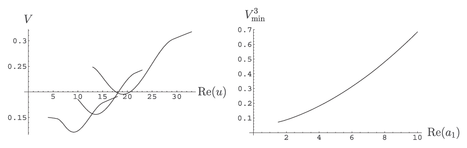
In this region, there are again three singular points and correspondingly three potential minima, at (left dyon), at (right dyon) and at (quark). Fig. 5 shows the effective potential along the real axis around the right dyon and the quark singular points for several values of . We note that the energy at the potential minimum is not zero expect certain point. The evolutions of the two minima at the right dyon and the quark singular points and are depicted in Fig. 6. The potential energies and approach zero as is decreasing, while the evolution of the potential energy at the singular point is the same as for . Thus, there are runaway directions along the flow of the right dyon and the quark singular points. We can find the same global structure along the flows of these two singular points for general complex values.
The evolutions of the potential energies according the flows of the singular points along the real -axis are simultaneously plotted in Fig. 7. The theory has SUSY vacua at and infinity, and no (local) SUSY breaking vacuum. However, this analysis gives us an important piece of information. In the presence of the soft term (4.2), the gauge dynamics favors the monopole and the dyon points at as SUSY vacua besides the runaway vacua. It implies that if we can add certain terms to (4.2) which produce a vacuum at a point different from at the classical level, SUSY is dynamically broken as a consequence of the discrepancy of SUSY conditions between the classical and the quantum theories. Actually, turning on the mass and the FI parameter realizes such a situation. In this case, the classical vacuum is at , different from the point which the dynamics favors. A resultant SUSY breaking vacuum is realized at non-zero value of . This is very similar to the SUSY breaking mechanism discussed in the Izawa-Yanagida-Intriligator-Thomas model in SUSY gauge theory [5, 6]. We show a schematic picture of our situation in Fig. 8.


Let us see in detail how this works for non-zero values of and . First we investigate the case . Fig. 9 shows the evolution of the potential energies at the monopole point for several values of as a function of with . The potential minimum is no longer realized at , but the location is shifted to negative values of as is expected from the discussion in the previous paragraph (see also Fig. 8). Furthermore, the potential energy has a non-zero value and therefore SUSY is dynamically broken. The potential energy becomes large as is increasing. This is expected from the fact that the effective potential behaves as (see (3.32) and (3.44)). We also find that the potential minimum at the monopole point is stable for general complex values of (for the case, see Fig. 3).
The same situation occurs at the degenerate dyon singular point. Recall that for vanishing and the theory has vacua at the degenerate dyon point and at the monopole point . These two vacua are transformed into each other under the symmetry . Since turning on and does not break this symmetry, it is also expected that SUSY is dynamically broken at the degenerate dyon point as it is shifted towards the negative direction of . Therefore we now have two SUSY breaking minima at the degenerate dyon point and at the monopole point.
In order to see the global structure of the effective potential we also need to investigate the potential for . Fig. 10 shows the potential energy around the quark singular point as a function of and the evolution of as a function of with and . Notably, the potential energy becomes large as is increasing. This behavior is completely different from the one of the case. This difference can be understood from the classical potential (2.4). Since we are considering the Coulomb branch, substitute (2) with into (2.4). Then we obtain
| (4.3) |
For large values of the term is dominant. Therefore the potential energy increases monotonically with growing . We find that the potential energies at the left and right dyon singular points also have the same structure.
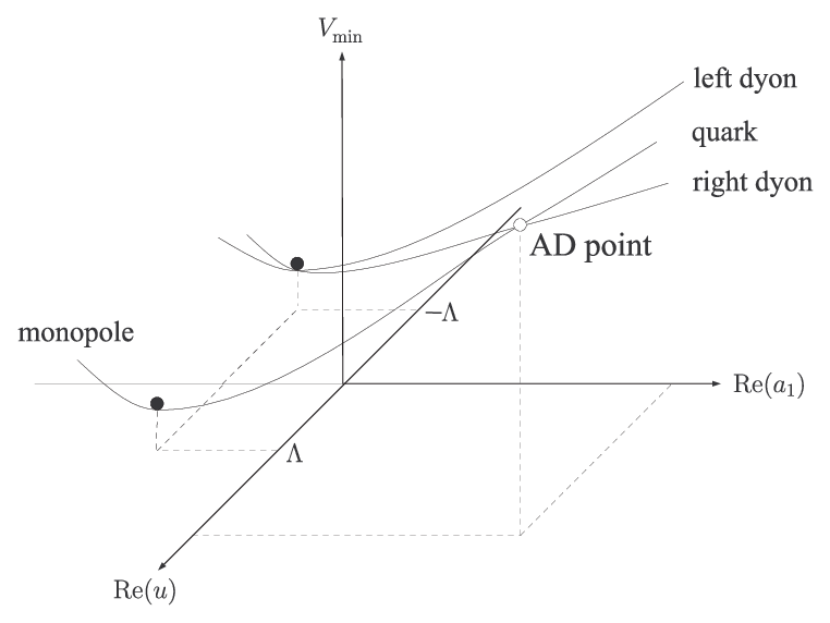
A qualitative picture of the evolutions of the potential minima is depicted in Fig. 11.
Now we have seen that there are two SUSY breaking minima and that there is no longer any runaway direction on the Coulomb branch. It appears that the two SUSY breaking minima are global ones, but there is still a possible SUSY vacuum on the Higgs branch whose existence in the classical theory is shown in (2.14). It is known that there are no quantum corrections on the Higgs branch [35]. Thus, at the quantum level, the SUSY vacuum on the Higgs branch is still left. In the next section, we discuss the decay rate from the local SUSY breaking vacua at the monopole and dyon singular points to the SUSY vacuum on the Higgs branch and show that the local vacua can actually be meta-stable with an appropriate choice of parameters.
5 Decay rate of the local vacuum
In this section, we estimate the decay rate from the SUSY breaking local minima on the Coulomb branch to the SUSY vacuum on the Higgs branch.
The local minimum at the monopole point on the Coulomb branch is approximately given by the point while the Higgs SUSY vacuum is at , (2.14) (see Fig. 12).

The distance between the vacua at Coulomb and Higgs branches, , is given by
| (5.4) |
We parameterize a point between and by the vector
where . The parameter value corresponds to the Coulomb vacuum while corresponds to the Higgs vacuum. Substituting (5) into the classical potential (2.4), we have
| (5.14) |
where
| (5.15) |
Now we show that there is a reasonable parameter region in which the local vacuum at the Coulomb branch, , is meta-stable. We take the following parameter region, and , so that
| (5.16) |
where we have neglected the second term in because of the small gauge coupling . Under eq. (5.16), the maximum value of the potential between and is located at and its value is given by
| (5.17) |
Since the SUSY breaking scale is estimated to be , we have
| (5.18) |
Thus we can use the thin-wall approximation to estimate the decay rate [36].
The bounce action is evaluated in the triangle approximation [37]
| (5.19) |
where in our case. The relevant quantities in the calculation are
| (5.20) |
Then the bounce action is evaluated to be , and the decay rate is extremely small. Therefore, the SUSY breaking vacuum at the monopole point is meta-stable. The decay rate from the degenerate dyon point to the SUSY vacuum and the one from the monopole point is the same due to the symmetric property in -direction (see fig.11).
6 Conclusion and discussion
We investigated an supersymmetric gauge theory with massless flavors. It contains soft terms, displayed in eq. (2.3), mass terms for and which break the SUSY down to and a term (a Fayet-Iliopoulos term) linear in .
We argued that when the parameters in the soft terms are small compared to the dynamical scale we can perform a reliable non-perturbative analysis based on the Seiberg-Witten solution. Our analysis revealed an interesting setup: On the Coulomb branch SUSY is dynamically broken in a manner reminiscent of the Izawa-Yanagida-Intriligator-Thomas model. A local minimum emerges, but no runaway SUSY vacua survive. On the Higgs branch, however, the SUSY vacua present at tree level should survive quantum corrections. The local minimum on the Coulomb branch decays into the Higgs branch vacuum, but not surprisingly, the values of the parameters can be chosen such that it is very long-lived, i.e. meta-stable.
It is interesting to discuss the symmetry. In some class of models possessing a meta-stable SUSY breaking vacuum, an approximate symmetry exists. In our model, at the classical level the theory has an approximate symmetry since we have taken the parameters in (2.3) to be small. However, the symmetry is broken to a discrete subgroup at the quantum level even if there are no small superpotential perturbations. Therefore, the theory does not have an approximate symmetry at the quantum level, so that the discussion in [39] cannot be applied to our case.
We would also like to comment on the difference between the models in this paper and in our previous paper [26]. Apart from the obvious difference that in this paper we start from a Lagrangian without extended SUSY, the pattern of vacuum states shows interesting differences: In [26], the theory has SUSY vacua only on the Higgs branch while on the Coulomb branch the potential has pseudo flat directions at the classical level. We found that after taking all the quantum corrections into account the effective potential exhibited a SUSY breaking local minimum. In the present case, a SUSY vacuum exists on the Coulomb branch at the classical level. We showed that the SUSY vacua are lifted by the gauge dynamics and revealed the mechanism how SUSY is dynamically broken.
In this paper, we chose a model simple enough to be able to perform a thorough analysis. As such, it is too poor to serve as a basis for any realistic phenomenology. However, we think that it once again shows the richness of supersymmetric gauge theories in being able to provide instances of the most different kinds of properties, and in this respect we hope that our simple model, like our previous attempt [26], could provide clues for building realistic descriptions of a world with broken supersymmetry.
Acknowledgements
The work of N. O. is partly supported by the Grant-in-Aid for Scientific Research in Japan (#15740164) and the Academy of Finland Finnish-Japanese Core Programme grant 112420. N.O. would also like to thank the High Energy Physics Division of the Department of Physical Sciences, University of Helsinki, for their hospitality during his visit. S. S. is supported by the bilateral program of Japan Society for the Promotion of Science and Academy of Finland, “Scientist Exchanges.”
Appendix
Appendix A Explicit form of the effective couplings
In this appendix, we show the explicit forms of the periods , the effective couplings and other quantities such as . They are necessary for the analysis of the potential (3.44) since the potential is a function of them. A more detailed derivation of these expressions can be found in [27, 26]. In the following, is a dynamical scale and is a common mass for the hypermultiplets, which is replaced with through the relation in the main body of the paper.
We first consider the periods and . Let us denote these as and respectively. These are given by
| (A.1) |
with the elliptic integrals explicitly given by
| (A.2) | |||||
| (A.3) | |||||
| (A.4) |
where , , , and . Here is a root of the elliptic curve for the QCD with massive flavors
| (A.5) | |||||
The formulae for are obtained from by exchanging the roots and . In eqs. (A.2)-(A.4), , and are the complete elliptic integrals [38] given by
| (A.6) | |||||
Next let us consider the effective coupling defined in eq. (3.4). The effective couplings and are obtained by
| (A.7) | |||||
| (A.8) |
where is the period of the Abelian differential,
| (A.9) |
and is defined as
| (A.10) |
Here is the incomplete elliptic integral of the first kind given by
| (A.11) |
The effective coupling is described in terms of the Weierstrass function
| (A.12) |
Here is the Weierstrass sigma function, and is the constant in eq. (3.18).
We now define the Landau pole associated with the interaction. In the ultraviolet region far away from the origin of the moduli space, the effective coupling is dominated by the gauge interaction since the interaction is asymptotic free and small. As expected, the gauge coupling is found to be a monotonically decreasing function of the large with fixed , and vice versa. The Landau pole is defined as at which . The large required in our assumption is realized by taking an appropriate value for . In this paper, we fix , which corresponds to in units of [27, 26]. Fig. 13 shows the plot of the effective coupling for as a function of with . The cusps appear through the effect of the dynamics; their locations are specified by (4.1).

Finally we give the forms of and . The former can be calculated as
| (A.13) | |||||
The latter is simply given by
| (A.14) |
References
- [1] E. Witten, Phys. Lett. B 105 (1981) 267.
- [2] J. Wess and B. Zumino, Phys. Lett. B 49 (1974) 52; S. Ferrara, J. Iliopoulos and B. Zumino, Nucl. Phys. B 77 (1974) 413; M. T. Grisaru, W. Siegel and M. Rocek, Nucl. Phys. B 159 (1979) 429.
- [3] N. Seiberg, Phys. Lett. B 318 (1993) 469 [arXiv:hep-ph/9309335].
- [4] N. Seiberg, Phys. Rev. D 49 (1994) 6857 [arXiv:hep-th/9402044].
- [5] K. I. Izawa and T. Yanagida, Prog. Theor. Phys. 95 (1996) 829 [arXiv:hep-th/9602180].
- [6] K. A. Intriligator and S. D. Thomas, Nucl. Phys. B 473 (1996) 121 [arXiv:hep-th/9603158].
- [7] K. Intriligator, N. Seiberg and D. Shih, JHEP 0604 (2006) 021 [arXiv:hep-th/0602239].
- [8] M. Dine and J. Mason, Phys. Rev. D 77 (2008) 016005 [arXiv:hep-ph/0611312].
- [9] C. Csaki, Y. Shirman and J. Terning, JHEP 0705 (2007) 099 [arXiv:hep-ph/0612241].
- [10] O. Aharony and N. Seiberg, JHEP 0702 (2007) 054 [arXiv:hep-ph/0612308].
- [11] R. Kitano, H. Ooguri and Y. Ookouchi, Phys. Rev. D 75 (2007) 045022 [arXiv:hep-ph/0612139].
- [12] H. Murayama and Y. Nomura, Phys. Rev. Lett. 98 (2007) 151803 [arXiv:hep-ph/0612186].
- [13] D. Shih, [arXiv:hep-th/0703196].
- [14] K. Intriligator, N. Seiberg and D. Shih, JHEP 0707 (2007) 017 [arXiv:hep-th/0703281].
- [15] L. Ferretti, JHEP 0712 (2007) 064 [arXiv:0705.1959 [hep-th]].
- [16] S. P. de Alwis, Phys. Rev. D 76 (2007) 086001 [arXiv:hep-th/0703247].
- [17] A. Katz, Y. Shadmi and T. Volansky, JHEP 0707 (2007) 020 [arXiv:0705.1074 [hep-th]].
- [18] S. Abel, C. Durnford, J. Jaeckel and V. V. Khoze, [arXiv:0707.2958 [hep-ph]].
- [19] N. Haba and N. Maru, Phys. Rev. D 76 (2007) 115019 [arXiv:0709.2945 [hep-ph]].
- [20] M. Dine and J. D. Mason, [arXiv:0712.1355 [hep-ph]].
- [21] A. Amariti, L. Girardello and A. Mariotti, JHEP 0612 (2006) 058 [arXiv:hep-th/0608063].
- [22] A. Amariti, L. Girardello and A. Mariotti, JHEP 0710 (2007) 017 [arXiv:0706.3151 [hep-th]].
- [23] A. Amariti, D. Forcella, L. Girardello and A. Mariotti, arXiv:0803.0514 [hep-th].
- [24] N. Seiberg and E. Witten, Nucl. Phys. B 426 (1994) 19 [Erratum-ibid. B 430 (1994) 485] [arXiv:hep-th/9407087].
- [25] N. Seiberg and E. Witten, Nucl. Phys. B 431 (1994) 484 [arXiv:hep-th/9408099].
- [26] M. Arai, C. Montonen, N. Okada and S. Sasaki, Phys. Rev. D 76 (2007) 125009 [arXiv:0708.0668 [hep-th]].
- [27] M. Arai and N. Okada, Phys. Rev. D 64 (2001) 025024 [arXiv:hep-th/0103157]; Nucl. Phys. Proc. Suppl. 102 (2001) 219 [arXiv:hep-th/0103174].
- [28] H. Ooguri, Y. Ookouchi and C. S. Park, [arXiv:0704.3613 [hep-th]].
- [29] G. Pastras, “Non supersymmetric metastable vacua in N = 2 SYM softly broken to N = 1,” arXiv:0705.0505 [hep-th].
- [30] J. Marsano, H. Ooguri, Y. Ookouchi and C. S. Park, [arXiv:0712.3305 [hep-th]].
- [31] L. Mazzucato, Y. Oz and S. Yankielowicz, JHEP 0711 (2007) 094 [arXiv:0709.2491 [hep-th]].
- [32] I. Bena, E. Gorbatov, S. Hellerman, N. Seiberg and D. Shih, JHEP 0611 (2006) 088 [arXiv:hep-th/0608157].
- [33] L. Alvarez-Gaume, M. Marino and F. Zamora, Int. J. Mod. Phys. A 13 (1998) 403 [arXiv:hep-th/9703072]; Int. J. Mod. Phys. A 13 (1998) 1847 [arXiv:hep-th/9707017].
- [34] P. C. Argyres and M. R. Douglas, Nucl. Phys. B 448 (1995) 93 [arXiv:hep-th/9505062].
- [35] P. C. Argyres, M. R. Plesser and N. Seiberg, Nucl. Phys. B 471 (1996) 159 [arXiv:hep-th/9603042].
- [36] S. R. Coleman, Phys. Rev. D 15 (1977) 2929 [Erratum-ibid. D 16 (1977) 1248].
- [37] M. J. Duncan and L. G. Jensen, Phys. Lett. B 291 (1992) 109.
- [38] A. Erdelyi et al., Higher Transcendental Functions, Vol. 1, McGraw-Hill, New York (1953).
- [39] K. Intriligator and N. Seiberg, Class. Quant. Grav. 24 (2007) S741 [arXiv:hep-ph/0702069].