跳到论文正文
W Papers独立论文阅读器 arXiv:0712.4091 论文正文 计算阅读时间 · 0%
引用这篇论文根据当前论文元数据生成,正式投稿前建议核对。


License: Assumed arXiv.org perpetual non-exclusive license
arXiv:0712.4091v2 [math-ph] 03 Jan 2008

Exact solution of the six-vertex model with domain wall boundary conditions. Ferroelectric phaseThanks: The first author is supported in part by the National Science Foundation (NSF) Grant DMS-0652005.

Pavel Bleher Address: Department of Mathematical Sciences, Indiana University-Purdue University Indianapolis, 402 N. Blackford St., Indianapolis, IN 46202, U.S.A. Email address: bleher@math.iupui.edu and Karl Liechty Address: Department of Mathematical Sciences, Indiana University-Purdue University Indianapolis, 402 N. Blackford St., Indianapolis, IN 46202, U.S.A. Email address: kliechty@math.iupui.edu
Date: August 11, 2026
Abstract.

This is a continuation of the paper [4] of Bleher and Fokin, in which the large nn asymptotics is obtained for the partition function ZnZ_{n} of the six-vertex model with domain wall boundary conditions in the disordered phase. In the present paper we obtain the large nn asymptotics of ZnZ_{n} in the ferroelectric phase. We prove that for any ε>0\varepsilon>0, as n→∞n\to\infty, Zn=C​Gn​Fn2​[1+O⁡(e−n1−ε)]Z_{n}=CG^{n}F^{n^{2}}[1+O(e^{-n^{1-\varepsilon}})], and we find the exact values of the constants C,GC,G and FF. The proof is based on the large nn asymptotics for the underlying discrete orthogonal polynomials and on the Toda equation for the tau-function.

1. Introduction and formulation of the main result

1.1. Definition of the model

The six-vertex model, or the model of two-dimensional ice, is stated on a square n×nn\times n lattice with arrows on edges. The arrows obey the rule that at every vertex there are two arrows pointing in and two arrows pointing out. Such rule is sometimes called the ice-rule. There are only six possible configurations of arrows at each vertex, hence the name of the model, see Fig. 1.

Refer to caption
Figure 1. The six arrow configurations allowed at a vertex.

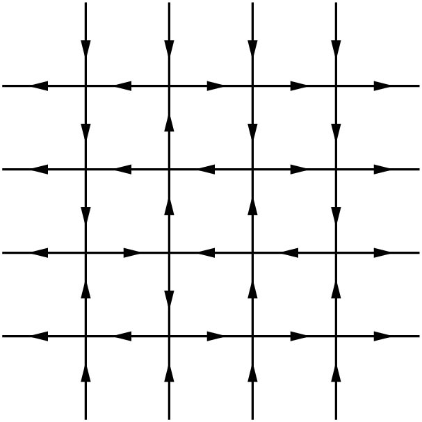
We will consider the domain wall boundary conditions (DWBC), in which the arrows on the upper and lower boundaries point in the square, and the ones on the left and right boundaries point out. One possible configuration with DWBC on the 4×44\times 4 lattice is shown on Fig. 2.

Refer to caption
Figure 2. An example of 4×44\times 4 configuration with DWBC.

For each possible vertex state we assign a weight wi,i=1,…,6w_{i},\;i=1,\dots,6, and define, as usual, the partition function as a sum over all possible arrow configurations of the product of the vertex weights,

Zn=∑arrow​configurations​σw⁡(σ),w⁡(σ)=∏x∈Vnwt⁡(x,σ)=∏i=16wiNi​(σ),Z_{n}=\sum_{{\rm arrow\;configurations}\;\sigma}w(\sigma),\qquad w(\sigma)=\prod_{x\in V_{n}}w_{t(x;\sigma)}=\prod_{i=1}^{6}w_{i}^{N_{i}(\sigma)}, (1.1)

where VnV_{n} is the n×nn\times n set of vertices, t⁡(x,σ)∈{1,…,6}t(x;\sigma)\in\{1,\ldots,6\} is the type of configuration σ\sigma at vertex xx according to Fig. 1, and Ni​(σ)N_{i}(\sigma) is the number of vertices of type ii in the configuration σ\sigma. The sum is taken over all possible configurations obeying the given boundary condition. The Gibbs measure is defined then as

μn​(σ)=w⁡(σ)Zn.\mu_{n}(\sigma)=\frac{w(\sigma)}{Z_{n}}\,. (1.2)

Our main goal is to obtain the large nn asymptotics of the partition function ZnZ_{n}.

The six-vertex model has six parameters: the weights wiw_{i}. By using some conservation laws it can be reduced to only two parameters. It is convenient to derive the conservation laws from the height function.

1.2. Height function

Consider the dual lattice,

V′={x=(i+12,j+12),0≤i,j≤n}.V^{\prime}=\{x=(i+\frac{1}{2},j+\frac{1}{2}),\quad 0\leq i,j\leq n\}. (1.3)

Given a configuration σ\sigma on EE, an integer-valued function h=hσh=h_{\sigma} on V′V^{\prime} is called a height function of σ\sigma, if for any two neighboring points x,y∈V′x,y\in V^{\prime}, |x−y|=1|x-y|=1, we have that

h⁡(y)−h⁡(x)=(−1)s,h(y)-h(x)=(-1)^{s}, (1.4)

where s=0s=0 if the arrow σe\sigma_{e} on the edge e∈Ee\in E, crossing the segment [x,y][x,y], is oriented in such a way that it points from left to right with respect to the vector x​y→\vec{xy} , and s=1s=1 if σe\sigma_{e} is oriented from right to left with respect to x​y→\vec{xy}. The ice-rule ensures that the height function h=hσh=h_{\sigma} exists for any configuration σ\sigma. It is unique up to addition of a constant. Fig. 3 shows a 5×55\times 5 configuration with a height function, and the corresponding alternating sign matrix, which is obtained from the configuration by replacing the vertex (5) of Fig. 1 by 1, the vertex (6) by (−1)(-1), and all the other vertices by 0.

Refer to caption
Figure 3. A 5×55\times 5 configuration with a height function and the corresponding alternating sign matrix.

Observe that if h1​(x),h2​(x),h3​(x),h4​(x)h_{1}(x),h_{2}(x),h_{3}(x),h_{4}(x) are the four values of the height function around a vertex x=(j,k)x=(j,k), enumerated in the positive direction around xx starting from the first quadrant, then the value of the element aj​ka_{jk} of the ASM is equal to

aj​k=h1​(x)−h2​(x)+h3​(x)−h4​(x)2.a_{jk}=\frac{h_{1}(x)-h_{2}(x)+h_{3}(x)-h_{4}(x)}{2}\,. (1.5)

1.3. Conservation laws

Conservation laws are obtained in the paper [12] of Ferrari and Spohn, as a corollary of a path representation of the six-vertex model. We will derive them from the height function representation. Consider the height function h=hσh=h_{\sigma} on a diagonal sequence of points defined by the formula,

xj=x0+(j,j),0≤j≤k,x_{j}=x_{0}+(j,j),\quad 0\leq j\leq k, (1.6)

where both x0x_{0} and xkx_{k} lie on the boundary B′B^{\prime} of the dual lattice V′V^{\prime},

B′\displaystyle B^{\prime} ={x=(i+12,12), 0≤i≤n}∪{x=(m+12,j+12), 0≤j≤n}\displaystyle=\{x=(i+\frac{1}{2},\frac{1}{2}),\;0\leq i\leq n\}\cup\{x=(m+\frac{1}{2},j+\frac{1}{2}),\;0\leq j\leq n\} (1.7)
∪{x=(i+12,n+12), 0≤i≤n}∪{x=(12,j+12), 0≤j≤n}.\displaystyle\cup\{x=(i+\frac{1}{2},n+\frac{1}{2}),\;0\leq i\leq n\}\cup\{x=(\frac{1}{2},j+\frac{1}{2}),\;0\leq j\leq n\}.

Then it follows from the definition of the height function, that

h(xj)−h(xj−1)={2,ift⁡(x,σ)=3,−2,ift⁡(x,σ)=4,0,ift⁡(x,σ)=1,2,5,6,h(x_{j})-h(x_{j-1})=\left\{\begin{aligned} &2,\quad{\rm if}\quad t(x;\sigma)=3,\\ &-2,\quad{\rm if}\quad t(x;\sigma)=4,\\ &0,\quad{\rm if}\quad t(x;\sigma)=1,2,5,6,\end{aligned}\right. (1.8)

where

x=xj+xj−12.x=\frac{x_{j}+x_{j-1}}{2}\,. (1.9)

Hence

0=h⁡(xk)−h⁡(x0)=2​N3​(σ,L)−2​N4​(σ,L),0=h(x_{k})-h(x_{0})=2N_{3}(\sigma;L)-2N_{4}(\sigma;L), (1.10)

where Ni​(σ,L)N_{i}(\sigma;L) is the number of vertex states of type ii in σ\sigma on the line

L={x=x0+(t,t),t∈ℝ}.L=\{x=x_{0}+(t,t),\;t\in{\mathbb{R}}\}. (1.11)

The line LL is parallel to the diagonal y=xy=x. By summing up over all possible lines LL, we obtain that

N3​(σ)−N4​(σ)=0,N_{3}(\sigma)-N_{4}(\sigma)=0, (1.12)

where Ni​(σ)N_{i}(\sigma) is the total number of vertex states of the type ii in the configuration σ\sigma.

Similarly, by considering lines LL parallel to the diagonal y=−xy=-x, we obtain that

N1​(σ)−N2​(σ)=0.N_{1}(\sigma)-N_{2}(\sigma)=0. (1.13)

Also,

N5​(σ)−N6​(σ)=n,N_{5}(\sigma)-N_{6}(\sigma)=n, (1.14)

which follows if we consider lines LL parallel to the xx-axis.

The conservation laws allow to reduce the weights w1,…,w6w_{1},\ldots,w_{6} to 3 parameters. Namely, we have that

w1N1​w2N2​w3N3​w4N4​w5N5​w6N6=C⁡(n)​aN1​aN2​bN3​bN4​cN5​cN6,w_{1}^{N_{1}}w_{2}^{N_{2}}w_{3}^{N_{3}}w_{4}^{N_{4}}w_{5}^{N_{5}}w_{6}^{N_{6}}=C(n)a^{N_{1}}a^{N_{2}}b^{N_{3}}b^{N_{4}}c^{N_{5}}c^{N_{6}}, (1.15)

where

a=w1​w2,b=w3​w4,c=w5​w6,a=\sqrt{w_{1}w_{2}},\quad b=\sqrt{w_{3}w_{4}},\quad c=\sqrt{w_{5}w_{6}}, (1.16)

and the constant

C⁡(n)=(w5w6)n2.C(n)=\left(\frac{w_{5}}{w_{6}}\right)^{\frac{n}{2}}\,. (1.17)

This implies the relation between the partition functions,

Zn​(w1,w2,w3,w4,w5,w6)=C⁡(n)​Zn​(a,a,b,b,c,c),Z_{n}(w_{1},w_{2},w_{3},w_{4},w_{5},w_{6})=C(n)Z_{n}(a,a,b,b,c,c), (1.18)

and between the Gibbs measures,

μn​(σ,w1,w2,w3,w4,w5,w6)=μn​(σ,a,a,b,b,c,c).\mu_{n}(\sigma;w_{1},w_{2},w_{3},w_{4},w_{5},w_{6})=\mu_{n}(\sigma;a,a,b,b,c,c). (1.19)

Therefore, for fixed boundary conditions, like DWBC, the general weights are reduced to the case when

w1=w2=a,w3=w4=b,w5=w6=c.w_{1}=w_{2}=a,\quad w_{3}=w_{4}=b,\quad w_{5}=w_{6}=c. (1.20)

Furthermore,

Zn​(a,a,b,b,c,c)=cn2​Zn​(ac,ac,bc,bc,1,1)Z_{n}(a,a,b,b,c,c)=c^{n^{2}}Z_{n}\left(\frac{a}{c},\frac{a}{c},\frac{b}{c},\frac{b}{c},1,1\right) (1.21)

and

μn​(σ,a,a,b,b,c,c)=μn​(σ,ac,ac,bc,bc,1,1),\mu_{n}(\sigma;a,a,b,b,c,c)=\mu_{n}\left(\sigma;\frac{a}{c},\frac{a}{c},\frac{b}{c},\frac{b}{c},1,1\right), (1.22)

so that a general weight reduces to the two parameters, ac,bc\frac{a}{c},\frac{b}{c}\,.

1.4. Exact solution of the six-vertex model for a finite nn

Introduce the parameter

Δ=a2+b2−c22​a​b.\Delta=\frac{a^{2}+b^{2}-c^{2}}{2ab}\,. (1.23)

There are three physical phases in the six-vertex model: the ferroelectric phase, Δ>1\Delta>1; the anti-ferroelectric phase, Δ<−1\Delta<-1; and, the disordered phase, −1<Δ<1-1<\Delta<1. In the three phases we parametrize the weights in the standard way: for the ferroelectric phase,

a=sinh⁡(t−γ),b=sinh⁡(t+γ),c=sinh⁡(2​|γ|),0<|γ|<t,a=\sinh(t-\gamma),\quad b=\sinh(t+\gamma),\quad c=\sinh(2|\gamma|),\quad 0<|\gamma|<t, (1.24)

for the anti-ferroelectric phase,

a=sinh⁡(γ−t),b=sinh⁡(γ+t),c=sinh⁡(2​γ),|t|<γ,a=\sinh(\gamma-t),\quad b=\sinh(\gamma+t),\quad c=\sinh(2\gamma),\quad|t|<\gamma, (1.25)

and for the disordered phase

a=sin⁡(γ−t),b=sin⁡(γ+t),c=sin⁡(2​γ),|t|<γ.a=\sin(\gamma-t),\quad b=\sin(\gamma+t),\quad c=\sin(2\gamma),\quad|t|<\gamma. (1.26)

The phase diagram of the six-vertex model is shown on Fig. 4.

Refer to caption
Figure 4. The phase diagram of the model, where F, AF and D mark ferroelectric, antiferroelectric, and disordered phases, respectively. The circular arc corresponds to the so-called ”free fermion” line, when Δ=0\Delta=0, and the three dots correspond to 1-, 2-, and 3-enumeration of alternating sign matrices.

The phase diagram and the Bethe-Ansatz solution of the six-vertex model for periodic and anti-periodic boundary conditions are thoroughly discussed in the works of Lieb [21]-[24], Lieb, Wu [25], Sutherland [30], Baxter [2], Batchelor, Baxter, O’Rourke, Yung [3]. See also the work of Wu, Lin [31], in which the Pfaffian solution for the six-vertex model with periodic boundary conditions is obtained on the free fermion line, Δ=0\Delta=0.

As concerns the six-vertex model with DWBC, it is noticed by Kuperberg [20], that on the diagonal,

ac=bc=x,\frac{a}{c}=\frac{b}{c}=x, (1.27)

the six-vertex model with DWBC is equivalent to the ss-enumeration of alternating sign matrices (ASM), in which the weight of each such matrix is equal to sN−s^{N_{-}}, where N−N_{-} is the number of (−1)(-1)’s in the matrix and s=1x2s=\frac{1}{x^{2}}. The exact solution for a finite nn is known for 1-, 2-, and 3-enumerations of ASMs, see the works by Kuperberg [20] and Colomo-Pronko [9] for a solution based on the Izergin-Korepin formula. A fascinating story of the discovery of the ASM formula is presented in the book [7] of Bressoud. On the free fermion line, γ=π4\gamma=\frac{\pi}{4}, the partition function of the six-vertex model with DWBC has a very simple form: Zn=1Z_{n}=1. For a nice short proof of this formula see the work [9] of Colomo-Pronko.

Here we will discuss the ferroelectric phase, and we will use parametrization (1.24). Without loss of generality we may assume that

γ>0,\gamma>0, (1.28)

which corresponds to the region,

b>a+c.b>a+c. (1.29)

The parameter Δ\Delta in the ferroelectric phase reduces to

Δ=cosh⁡(2​γ).\Delta=\cosh(2\gamma). (1.30)

The six-vertex model with DWBC was introduced by Korepin in [16], who derived an important recursion relation for the partition function of the model. This lead to a beautiful determinantal formula of Izergin [13] for the partition function with DWBC. A detailed proof of this formula and its generalizations are given in the paper of Izergin, Coker, and Korepin [14]. When the weights are parameterized according to (1.24), the formula of Izergin is

Zn=[sinh⁡(t−γ)​sinh⁡(t+γ)]n2(∏j=0n−1j!)2​τn,Z_{n}=\frac{[\sinh(t-\gamma)\sinh(t+\gamma)]^{n^{2}}}{\left(\prod_{j=0}^{n-1}j!\right)^{2}}\,\tau_{n}\,, (1.31)

where τn\tau_{n} is the Hankel determinant,

τn=det(dj+k−2​ϕd​tj+k−2)1≤j,k≤n,\tau_{n}=\det\left(\frac{d^{j+k-2}\phi}{dt^{j+k-2}}\right)_{1\leq j,k\leq n}, (1.32)

and

ϕ⁡(t)=sinh⁡(2​γ)sinh⁡(t+γ)​sinh⁡(t−γ).\phi(t)=\frac{\sinh(2\gamma)}{\sinh(t+\gamma)\sinh(t-\gamma)}\,. (1.33)

An elegant derivation of the Isergin determinantal formula from the Yang-Baxter equation is given in the papers of Korepin, Zinn-Justin [19] and Kuperberg [20] (see also the book of Bressoud [7]).

One of the applications of the determinantal formula is that it implies that the partition function τn\tau_{n} solves the Toda equation

τnτn′′−τn′2=τn+1τn−1,n≥1,()′=∂∂t,\tau_{n}\tau^{\prime\prime}_{n}-{\tau^{\prime}_{n}}^{2}=\tau_{n+1}\tau_{n-1},\qquad n\geq 1,\qquad({}^{\prime})=\frac{\partial}{\partial t}\,, (1.34)

cf. the work of Sogo, [27]. The Toda equation was used by Korepin and Zinn-Justin [19] to derive the free energy of the six-vertex model with DWBC, assuming some Ansatz on the behavior of subdominant terms in the large NN asymptotics of the free energy.

Another application of the Izergin determinantal formula is that τN\tau_{N} can be expressed in terms of a partition function of a random matrix model and also in terms of related orthogonal polynomials, see the paper [32] of Zinn-Justin. In the ferroelectric phase the expression in terms of orthogonal polynomials can be obtained as follows. For the evaluation of the Hankel determinant, let us write ϕ⁡(t)\phi(t) in the form of the Laplace transform of a discrete measure,

ϕ⁡(t)=sinh⁡(2​γ)sinh⁡(t+γ)​sinh⁡(t−γ)=4​∑l=1∞e−2​t​l​sinh⁡(2​γ​l).\phi(t)=\frac{\sinh(2\gamma)}{\sinh(t+\gamma)\sinh(t-\gamma)}=4\sum_{l=1}^{\infty}e^{-2tl}\sinh(2\gamma l). (1.35)

Then

τn=2n2n!​∑l1,…,ln=1∞Δ​(li)2​∏i=1n[2​e−2​t​li​sinh⁡(2​γ​li)],\tau_{n}=\frac{2^{n^{2}}}{n!}\sum_{l_{1},\ldots,l_{n}=1}^{\infty}\Delta(l_{i})^{2}\prod_{i=1}^{n}\left[2e^{-2tl_{i}}\sinh(2\gamma l_{i})\right], (1.36)

where

Δ⁡(li)=∏1≤i<j≤n(lj−li)\Delta(l_{i})=\prod_{1\leq i<j\leq n}(l_{j}-l_{i}) (1.37)

is the Vandermonde determinant.

Introduce now discrete monic polynomials Pj​(x)=xj+…P_{j}(x)=x^{j}+\dots orthogonal on the set ℕ={l=1,2,…}{\mathbb{N}}=\{l=1,2,\ldots\} with respect to the weight,

w⁡(l)=2​e−2​t​l​sinh⁡(2​γ​l)=e−2​t​l+2​γ​l−e−2​t​l−2​γ​l,w(l)=2e^{-2tl}\sinh(2\gamma l)=e^{-2tl+2\gamma l}-e^{-2tl-2\gamma l}, (1.38)

so that

∑l=1∞Pj​(l)​Pk​(l)​w​(l)=hk​δj​k.\sum_{l=1}^{\infty}P_{j}(l)P_{k}(l)w(l)=h_{k}\delta_{jk}. (1.39)

Then it follows from (1.36) that

τn=2n2​∏k=0n−1hk,\tau_{n}=2^{n^{2}}\prod_{k=0}^{n-1}h_{k}, (1.40)

see Appendix in the end of the paper. We will prove the following asymptotics of hkh_{k}.

Theorem 1.1.

For any ε>0\varepsilon>0, as k→∞k\to\infty,

hk=(k!)2​qk+1(1−q)2​k+1​(1+O⁡(e−k1−ε)),h_{k}=\frac{(k!)^{2}q^{k+1}}{(1-q)^{2k+1}}\,\left(1+O(e^{-k^{1-\varepsilon}})\right), (1.41)

where

q=e2​γ−2​t.q=e^{2\gamma-2t}. (1.42)

The error term in (1.41) is uniform on any compact subset of the set

{(t,γ): 0<γ<t}.\left\{(t,\gamma):\;0<\gamma<t\right\}. (1.43)

1.5. Main result: Asymptotics of the partition function

This work is a continuation of the work [4] of the first author with Vladimir Fokin. In [4] the authors obtain the large nn asymptotics of the partition function ZnZ_{n} in the disordered phase. They prove the conjecture of Paul Zinn-Justin [32] that the large nn asymptotics of ZnZ_{n} in the disordered phase has the following form: for some ε>0\varepsilon>0,

Zn=C​nκ​Fn2​[1+O⁡(n−ε)],Z_{n}=Cn^{\kappa}F^{n^{2}}[1+O(n^{-\varepsilon})], (1.44)

and they find the exact value of the exponent κ\kappa,

κ=112−2​γ23​π​(π−2​γ).\kappa=\frac{1}{12}-\frac{2\gamma^{2}}{3\pi(\pi-2\gamma)}\,. (1.45)

The value of FF in the disordered phase is given by the formula,

F=π⁡[sin⁡(γ+t)​sin⁡(γ−t)]2​γ​cos⁡π​t2​γ,F=\frac{\pi[\sin(\gamma+t)\sin(\gamma-t)]}{2\gamma\cos\frac{\pi t}{2\gamma}}\,, (1.46)

the exact value of constant C>0C>0 is not yet known.

Our main result in the present paper is the following theorem.

Theorem 1.2.

In the ferroelectric phase with t>γ>0t>\gamma>0, for any ε>0\varepsilon>0, as n→∞n\to\infty,

Zn=C​Gn​Fn2​[1+O⁡(e−n1−ε)],Z_{n}=CG^{n}F^{n^{2}}\left[1+O\left(e^{-n^{1-\varepsilon}}\right)\right], (1.47)

where C=1−e−4​γC=1-e^{-4\gamma}, G=eγ−tG=e^{\gamma-t}, and F=sinh⁡(t+γ)F=\sinh(t+\gamma). The error term in (1.41) is uniform on any compact subset of the set (1.43).

Up to a constant factor this result will follow from Theorem 1.1. To find the constant factor CC we will use the Toda equation, combined with the asymptotics of CC as t→∞t\to\infty. The proof of Theorems 1.1 and 1.2 will be given below in Sections 2-6. Here we would like to make some remarks concerning the phase transition between the ferroelectric and disordered phases.

1.6. Order of the phase transition between the ferroelectric and disordered phases

We would like to compare the free energy in the disordered phase and in the ferroelectric phase, when we approach a point of phase transition. Consider first the ferroelectric phase. Observe that t,γ→0t,\gamma\to 0 as we approach the line of phase transition,

bc=ac+1,\frac{b}{c}=\frac{a}{c}+1, (1.48)

hence a,b,c→0a,b,c\to 0 in parametrization (1.24). Consider the regime,

t,γ→+0,tγ→α>1.t,\gamma\to+0,\qquad\frac{t}{\gamma}\to\alpha>1. (1.49)

In this regime,

limγ→0bc=limγ→0sinh⁡(t+γ)sinh⁡(2​γ)=α+12,limγ→0ac=limγ→0sinh⁡(t−γ)sinh⁡(2​γ)=α−12.\lim_{\gamma\to 0}\frac{b}{c}=\lim_{\gamma\to 0}\frac{\sinh(t+\gamma)}{\sinh(2\gamma)}=\frac{\alpha+1}{2}\,,\qquad\lim_{\gamma\to 0}\frac{a}{c}=\lim_{\gamma\to 0}\frac{\sinh(t-\gamma)}{\sinh(2\gamma)}=\frac{\alpha-1}{2}\,. (1.50)

We have to rescale formula (1.47) according to (1.21),

Zn​(ac,ac,bc,bc,1,1)=c−n2​Zn​(a,a,b,b,c,c)=C​Gn​F0n2​[1+O⁡(e−n1−ε)],Z_{n}\left(\frac{a}{c},\frac{a}{c},\frac{b}{c},\frac{b}{c},1,1\right)=c^{-n^{2}}Z_{n}(a,a,b,b,c,c)=CG^{n}F_{0}^{n^{2}}\left[1+O\left(e^{-n^{1-\varepsilon}}\right)\right], (1.51)

where

F0=Fc=sinh⁡(t+γ)sinh⁡(2​γ).F_{0}=\frac{F}{c}=\frac{\sinh(t+\gamma)}{\sinh(2\gamma)}\,. (1.52)

Similarly, in the disordered phase,

Zn​(ac,ac,bc,bc,1,1)=C​nκ​F0n2​[1+O⁡(n−ε)],Z_{n}\left(\frac{a}{c},\frac{a}{c},\frac{b}{c},\frac{b}{c},1,1\right)=Cn^{\kappa}F_{0}^{n^{2}}[1+O(n^{-\varepsilon})], (1.53)

where

F0=Fc=π​sin⁡(γ−t)​sin⁡(γ+t)2​γ​sin⁡(2​γ)​cos⁡π​t2​γ.F_{0}=\frac{F}{c}=\frac{\pi\sin(\gamma-t)\sin(\gamma+t)}{2\gamma\sin(2\gamma)\cos\frac{\pi t}{2\gamma}}\,. (1.54)

Observe that parametrization (1.26) in the disordered phase is not convenient as we approach critical line (1.48). Namely, it corresponds to the limit when

t,γ→π2−0,π2−tπ2−γ→α>1.t,\gamma\to\frac{\pi}{2}-0,\qquad\frac{\frac{\pi}{2}-t}{\frac{\pi}{2}-\gamma}\to\alpha>1. (1.55)

Therefore, we replace tt for π2−t\frac{\pi}{2}-t and γ\gamma for π2−γ\frac{\pi}{2}-\gamma. This gives the parametrization,

a=sin⁡(t−γ),b=sin⁡(t+γ),c=sin⁡(2​|γ|),|γ|<t.a=\sin(t-\gamma),\quad b=\sin(t+\gamma),\quad c=\sin(2|\gamma|),\quad|\gamma|<t. (1.56)

The approach to critical line (1.48) is described by regime (1.49). Formula (1.54) reads in the new t,γt,\gamma as

F0=π​sin⁡(t−γ)​sin⁡(t+γ)(π−2​γ)​sin⁡(2​γ)​cos⁡[π⁡(π2−t)2​(π2−γ)].F_{0}=\frac{\pi\sin(t-\gamma)\sin(t+\gamma)}{\left(\pi-2\gamma\right)\sin(2\gamma)\cos\left[\frac{\pi(\frac{\pi}{2}-t)}{2(\frac{\pi}{2}-\gamma)}\right]}\,. (1.57)

We consider F0F_{0} on the line

a+bc=α,\frac{a+b}{c}=\alpha, (1.58)

and we use the parameter

β=b−ac\beta=\frac{b-a}{c}\, (1.59)

on this line. In variables α,β\alpha,\beta,

F0=α+β2​in the ferroelectric phase,F_{0}=\frac{\alpha+\beta}{2}\;\;\textrm{in the ferroelectric phase}, (1.60)

and

F0=(α+β)​g​(t,γ)2​in the disordered phase,F_{0}=\frac{(\alpha+\beta)g(t,\gamma)}{2}\,\;\;\textrm{in the disordered phase}, (1.61)

where

g⁡(t,γ)=π​sin⁡(t−γ)(π−2​γ)​sin⁡[π⁡(t−γ)(π−2​γ)]g(t,\gamma)=\frac{\pi\sin(t-\gamma)}{\left(\pi-2\gamma\right)\sin\left[\frac{\pi(t-\gamma)}{(\pi-2\gamma)}\right]} (1.62)

A straightforward calculation shows that on the line a+bc=α\frac{a+b}{c}=\alpha in the disordered phase, as β→1−0\beta\to 1-0,

g⁡(t,γ)=1+2​(α−1)3/2​(1−β)3/23​π​(α+1)1/2+O⁡((1−β)2).g(t,\gamma)=1+\frac{2(\alpha-1)^{3/2}(1-\beta)^{3/2}}{3\pi(\alpha+1)^{1/2}}+O((1-\beta)^{2}). (1.63)

By (1.60), g⁡(t,γ)=1g(t,\gamma)=1 in the ferroelectric phase. This implies that the free energy F0F_{0} exhibits a phase transition of the order 32\frac{3}{2} with respect to the parameter β\beta at the point β=1\beta=1. Fig.5 depicts the graph of F0=F0​(β)F_{0}=F_{0}(\beta) (the left graph) and its derivative, F0′​(β)F_{0}^{\prime}(\beta) (the right graph), as a function of β=b−ac\beta=\frac{b-a}{c} on the line b+ac=2\frac{b+a}{c}=2. Observe the square root singularities of F0′F_{0}^{\prime} at β=±1\beta=\pm 1, which correspond to the phase transition of order 32.\frac{3}{2}\,. Since

Δ=a2+b2−c22​a​b=α2+β2−2α2−β2=1+4​(β−1)α2−1+O⁡((β−1)2),\Delta=\frac{a^{2}+b^{2}-c^{2}}{2ab}=\frac{\alpha^{2}+\beta^{2}-2}{\alpha^{2}-\beta^{2}}=1+\frac{4(\beta-1)}{\alpha^{2}-1}+O((\beta-1)^{2})\,, (1.64)

it is a phase transition of the order 32\frac{3}{2} as well, with respect to the parameter Δ\Delta at the point Δ=1\Delta=1.

Refer to caption
Refer to caption
Figure 5. Free energy F0=F0​(β)F_{0}=F_{0}(\beta) (the left graph) and its derivative (the right graph), as functions of β=b−ac\beta=\frac{b-a}{c} on the line b+ac=2\frac{b+a}{c}=2.

The set-up for the remainder of the article is the following. In Section 2 we will discuss the Meixner polynomials, which will serve as a good approximation to the polynomials Pn​(z)P_{n}(z). In Section 3 we will discuss the Riemann-Hilbert approach to discrete orthogonal polynomials, and we will derive a basic identity, which will be used in the proof of Theorem 1.1. In Section 4 we will prove Theorem 1.1. Then, in Sections 5 and 6 we will obtain an explicit formula for the constant factor CC, and we will finish the proof of Theorem 1.2. Finally, in Section 7 we will compare the asymptotics of the free energy in the ferroelectric phase with the energy of the ground state configuration.

2. Meixner polynomials

We will use the two weights: the weight w⁡(l)w(l) defined in (1.38) and the exponential weight on ℕ{\mathbb{N}},

wQ​(l)=ql,l∈ℕ;q=e2​γ−2​t<1,w^{\rm Q}(l)=q^{l},\quad l\in{\mathbb{N}};\qquad q=e^{2\gamma-2t}<1, (2.1)

which can be viewed as an approximation to w⁡(l)w(l) for large ll. The orthogonal polynomials with the weight wQ​(l)w^{\rm Q}(l) are expressed in terms of the Meixner polynomials with β=1\beta=1, which are defined by the formula,

Mk​(z,q)\displaystyle M_{k}(z;q) =F12​(−k,−z1,1−q−1)=∑j=0∞(−k)j​(−z)j(1)j​(1−q−1)jj!\displaystyle={}_{2}F_{1}\left(\begin{matrix}-k,-z\\ 1\end{matrix};1-q^{-1}\right)=\sum_{j=0}^{\infty}\frac{(-k)_{j}(-z)_{j}}{(1)_{j}}\,\frac{(1-q^{-1})^{j}}{j!} (2.2)
=∑j=0k(1−q−1)j​∏i=0j−1(k−i)​∏i=0j−1(z−i)(j!)2.\displaystyle=\sum_{j=0}^{k}\frac{(1-q^{-1})^{j}\prod_{i=0}^{j-1}(k-i)\prod_{i=0}^{j-1}(z-i)}{(j!)^{2}}\,.

They satisfy the orthogonality condition,

∑l=0∞Mj​(l,q)​Mk​(l,q)​ql=q−k​δj​k1−q,\sum_{l=0}^{\infty}M_{j}(l;q)M_{k}(l;q)q^{l}=\frac{q^{-k}\delta_{jk}}{1-q}\,, (2.3)

see, e.g. [18]. For the corresponding monic polynomials,

PkM​(z)=k!(1−q−1)k​Mk​(z,q)P_{k}^{\rm M}(z)=\frac{k!}{(1-q^{-1})^{k}}M_{k}(z;q) (2.4)

(M in PkMP_{k}^{\rm M} stands for Meixner), the orthogonality condition reads

∑l=0∞PjM​(l)​PkM​(l)​qj=hkM​δj​k,hkM=(k!)2​qk(1−q)2​k+1.\sum_{l=0}^{\infty}P_{j}^{\rm M}(l)P_{k}^{\rm M}(l)q^{j}=h_{k}^{\rm M}\delta_{jk},\qquad h_{k}^{\rm M}=\frac{(k!)^{2}q^{k}}{(1-q)^{2k+1}}\,. (2.5)

They satisfy the three term recurrence relation,

z​PkM​(z)=Pk+1M​(z)+k​q+k+q1−q​PkM​(z)+k2​q(1−q)2​Pk−1M​(z),zP_{k}^{\rm M}(z)=P_{k+1}^{\rm M}(z)+\frac{kq+k+q}{1-q}\,P_{k}^{\rm M}(z)+\frac{k^{2}q}{(1-q)^{2}}\,P_{k-1}^{\rm M}(z), (2.6)

see [18]. According to (3.8), we take q=e2​γ−2​tq=e^{2\gamma-2t}.

For our purposes it is convenient to introduce a shifted Meixner polynomial,

Qk​(z)=PkM​(z−1)=(−1)k​k!​qk(1−q)k​Mk​(z−1,q),Q_{k}(z)=P_{k}^{\rm M}(z-1)=\frac{(-1)^{k}k!q^{k}}{(1-q)^{k}}M_{k}(z-1;q), (2.7)

which is a monic polynomial as well. Equation (2.5) implies the orthogonality condition,

∑l=1∞Qj​(l)​Qk​(l)​ql=hkQ​δj​k,hkQ=(k!)2​qk+1(1−q)2​k+1.\sum_{l=1}^{\infty}Q_{j}(l)Q_{k}(l)q^{l}=h_{k}^{\rm Q}\delta_{jk},\qquad h_{k}^{\rm Q}=\frac{(k!)^{2}q^{k+1}}{(1-q)^{2k+1}}\,. (2.8)

By analogy with (1.40), define

τnQ=2n2​∏k=0n−1hkQ.\tau_{n}^{\rm Q}=2^{n^{2}}\prod_{k=0}^{n-1}h_{k}^{\rm Q}. (2.9)

From (2.5) and (2.8) we obtain that

τnQ=2n2​∏k=0n−1(k!)2​qk+1(1−q)2​k+1=2n2​q(n+1)​n/2(1−q)n2​∏k=0n−1(k!)2.\tau_{n}^{\rm Q}=2^{n^{2}}\prod_{k=0}^{n-1}\frac{(k!)^{2}q^{k+1}}{(1-q)^{2k+1}}=\frac{2^{n^{2}}q^{(n+1)n/2}}{(1-q)^{n^{2}}}\prod_{k=0}^{n-1}(k!)^{2}\,. (2.10)

By analogy with (1.31), define also

ZnQ=[sinh⁡(γ+t)​sinh⁡(γ−t)]n2∏k=0n−1(k!)2​τnQ.Z_{n}^{\rm Q}=\frac{[\sinh(\gamma+t)\sinh(\gamma-t)]^{n^{2}}}{\displaystyle\prod_{k=0}^{n-1}(k!)^{2}}\,\tau_{n}^{\rm Q}\,. (2.11)

Then from (2.10) we obtain that

ZnQ=Fn2​Gn,Z_{n}^{\rm Q}=F^{n^{2}}G^{n}, (2.12)

where

F=2​sinh⁡(t−γ)​sinh⁡(t+γ)​q1/21−q=2​sinh⁡(t−γ)​sinh⁡(t+γ)​eγ−t1−e2​γ−2​t=sinh⁡(t+γ),F=\frac{2\sinh(t-\gamma)\sinh(t+\gamma)q^{1/2}}{1-q}=\frac{2\sinh(t-\gamma)\sinh(t+\gamma)e^{\gamma-t}}{1-e^{2\gamma-2t}}=\sinh(t+\gamma), (2.13)

and

G=q1/2=eγ−t.G=q^{1/2}=e^{\gamma-t}. (2.14)

Our goal will be to compare the normalizing constants for orthogonal polynomials with the weights ww and wQw^{\rm Q}. To this end let us discuss the Riemann-Hilbert approach to discrete orthogonal polynomials.

3. Riemann Hilbert approach: Interpolation problem

The Riemann-Hilbert approach to discrete orthogonal polynomials is based on the following Interpolation Problem (IP), which was introduced in the paper [6] of Borodin and Boyarchenko under the name of the discrete Riemann-Hilbert problem. See also the monograph [5] of Baik, Kriecherbauer, McLaughlin, and Miller, in which it is called the Interpolation Problem. Let w⁡(l)≥0w(l)\geq 0 be a weight function on ℕ{\mathbb{N}} (it can be a more general discrete set, as discussed in [6] and [5], but we will need ℕ{\mathbb{N}} in our problem).

Interpolation Problem. For a given k=0,1,…k=0,1,\ldots, find a 2×22\times 2 matrix-valued function Y⁡(z,k)=(Yi​j​(z,k))1≤i,j≤2Y(z;k)=(Y_{ij}(z;k))_{1\leq i,j\leq 2} with the following properties:

  1. (1)

    Analyticity: Y⁡(z,k)Y(z;k) is an analytic function of zz for z∈ℂ∖ℕz\in{\mathbb{C}}\setminus{\mathbb{N}}.

  2. (2)

    Residues at poles: At each node l∈ℕl\in{\mathbb{N}}, the elements Y11​(z,k)Y_{11}(z;k) and Y21​(z,k)Y_{21}(z;k) of the matrix Y⁡(z,k)Y(z;k) are analytic functions of zz, and the elements Y12​(z,k)Y_{12}(z;k) and Y22​(z,k)Y_{22}(z;k) have a simple pole with the residues,

    Resz=lYj2(z;k)=w(l)Yj1(l;k),j=1,2.\underset{z=l}{\rm Res}\;Y_{j2}(z;k)=w(l)Y_{j1}(l;k),\quad j=1,2. (3.1)
  3. (3)

    Asymptotics at infinity: As z→∞z\to\infty, Y⁡(z,k)Y(z;k) admits the asymptotic expansion,

    Y⁡(z,k)∼(I+Y1z+Y2z2+…)​(zk00z−k),z∈ℂ∖[⋃l=1∞D⁡(l,rl)],Y(z;k)\sim\left(I+\frac{Y_{1}}{z}+\frac{Y_{2}}{z^{2}}+\ldots\right)\begin{pmatrix}z^{k}&0\\ 0&z^{-k}\end{pmatrix},\qquad z\in{\mathbb{C}}\setminus\left[\bigcup_{l=1}^{\infty}D(l,r_{l})\right], (3.2)

    where D⁡(z,r)D(z,r) is a disk of radius r>0r>0 centered at z∈ℂz\in{\mathbb{C}} and

    liml→∞rl=0.\lim_{l\to\infty}r_{l}=0. (3.3)

It is not difficult to see (see [6] and [5]) that under some conditions on w⁡(l)w(l), the IP has a unique solution, which is

Y⁡(z,k)=(Pk​(z)C​(w​Pk)​(z)(hk−1)−1​Pk−1​(z)(hk−1)−1​C​(w​Pk−1)​(z))Y(z;k)=\begin{pmatrix}P_{k}(z)&C(wP_{k})(z)\\ (h_{k-1})^{-1}P_{k-1}(z)&(h_{k-1})^{-1}C(wP_{k-1})(z)\end{pmatrix} (3.4)

where the Cauchy transformation CC is defined by the formula,

C⁡(f)​(z)=∑l=1∞f⁡(l)z−l,C(f)(z)=\sum_{l=1}^{\infty}\frac{f(l)}{z-l}\,, (3.5)

and Pk​(z)=zk+…P_{k}(z)=z^{k}+\ldots are monic polynomials orthogonal with the weight w⁡(l)w(l), so that

∑l=1∞Pj​(l)​Pk​(l)​w​(l)=hj​δj​k.\sum_{l=1}^{\infty}P_{j}(l)P_{k}(l)w(l)=h_{j}\delta_{jk}. (3.6)

It follows from (3.4), that

hk=[Y1]21,h_{k}=[Y_{1}]_{21}, (3.7)

where [Y1]21[Y_{1}]_{21} is the (21)-element of the matrix Y1Y_{1} on the right in (3.2). In what follows we will consider the solution Y⁡(z,k)Y(z;k) for the weight w⁡(l)w(l), introduced in (1.38).

Let YQY^{\rm Q} be a solution to the IP with the exponential weight wQw^{\rm Q},

YQ​(z,k)=(Qk​(z)C⁡(wQ​Qk)​(z)(hk−1Q)−1​Qk−1​(z)(hk−1Q)−1​C​(wQ​Qk−1)​(z)).Y^{\rm Q}(z;k)=\begin{pmatrix}Q_{k}(z)&C(w^{\rm Q}Q_{k})(z)\\ (h_{k-1}^{\rm Q})^{-1}Q_{k-1}(z)&(h_{k-1}^{\rm Q})^{-1}C(w^{\rm Q}Q_{k-1})(z)\end{pmatrix}. (3.8)

Consider the quotient matrix,

X⁡(z,k)=Y⁡(z,k)​[YQ​(z,k)]−1.X(z;k)=Y(z;k)[Y^{\rm Q}(z;k)]^{-1}. (3.9)

Observe that detYQ​(z,k)\det Y^{\rm Q}(z;k) has no poles and it approaches 1 as z→∞z\to\infty outside of the disks D⁡(l,rl)D(l,r_{l}), l=1,2,…l=1,2,\ldots, hence

detYQ​(z,k)=1.\det Y^{\rm Q}(z;k)=1. (3.10)

Also,

X(z;k)→Ias z→∞ outside of the disks D⁡(l,rl), l=1,2,…X(z;k)\to I\quad\textrm{as $z\to\infty$ outside of the disks $D(l,r_{l})$, $l=1,2,\ldots$} (3.11)

This implies that the matrix XX can be written as

X⁡(z,k)=I+C⁡[(wQ−w)​R],X(z;k)=I+C[(w^{\rm Q}-w)R], (3.12)

where

R⁡(z)=((hk−1Q)−1​Pk​(z)​Qk−1​(z)−Pk​(z)​Qk​(z)(hk−1​hk−1Q)−1​Pk−1​(z)​Qk−1​(z)−(hk−1)−1​Pk−1​(z)​Qk​(z)).R(z)=\begin{pmatrix}(h_{k-1}^{\rm Q})^{-1}P_{k}(z)Q_{k-1}(z)&-P_{k}(z)Q_{k}(z)\\ (h_{k-1}h_{k-1}^{\rm Q})^{-1}P_{k-1}(z)Q_{k-1}(z)&-(h_{k-1})^{-1}P_{k-1}(z)Q_{k}(z)\end{pmatrix}. (3.13)

From formula (3.7) and (3.12) we obtain that

hk−hkQ=−∑l=1∞Pk(l)Qk(l)[wQ(l)−w(l)].h_{k}-h_{k}^{\rm Q}=-\sum_{l=1}^{\infty}P_{k}(l)Q_{k}(l)\,[w^{\rm Q}(l)-w(l)]. (3.14)

We will use this identity to estimate |hk−hkQ||h_{k}-h_{k}^{\rm Q}|. Observe that formula (3.12) can be further used to evaluate the large nn asymptotics of the orthogonal polynomials Pn​(z)P_{n}(z), but we will not pursue it here.

We would like to remark that identity (3.14) can be also derived as follows. Observe that since PkP_{k} and QkQ_{k} are monic polynomials, the difference, Pk−QkP_{k}-Q_{k}, is a polynomial of degree less than kk, hence

∑l=1∞Pk​(l)​[Qk​(l)−Pk​(l)]​w​(l)=0.\sum_{l=1}^{\infty}P_{k}(l)[Q_{k}(l)-P_{k}(l)]w(l)=0. (3.15)

By adding this to equation (3.6) with j=kj=k, we obtain that

hk=∑l=1∞Pk​(l)​Qk​(l)​w​(l).h_{k}=\sum_{l=1}^{\infty}P_{k}(l)Q_{k}(l)w(l). (3.16)

Similarly, from (2.8) we obtain that

hkQ=∑l=1∞Pk​(l)​Qk​(l)​wQ​(l).h_{k}^{\rm Q}=\sum_{l=1}^{\infty}P_{k}(l)Q_{k}(l)w^{\rm Q}(l). (3.17)

By subtracting the last two equations, we obtain identity (3.14).

4. Evaluation of the ratio hk/hkQh_{k}/h_{k}^{\rm Q}

In this section we will prove Theorem 1.1. By applying the Cauchy-Schwarz inequality to identity (3.14), we obtain that

|hk−hkQ|≤[∑l=1∞Pk​(l)2​|w⁡(l)−wQ​(l)|]1/2​[∑l=1∞Qk​(l)2​|w⁡(l)−wQ​(l)|]1/2,|h_{k}-h_{k}^{\rm Q}|\leq\left[\sum_{l=1}^{\infty}P_{k}(l)^{2}\,|w(l)-w^{\rm Q}(l)|\right]^{1/2}\left[\sum_{l=1}^{\infty}Q_{k}(l)^{2}\,|w(l)-w^{\rm Q}(l)|\right]^{1/2}, (4.1)

so that

|hkhkQ−1|≤[1hkQ​∑l=1∞Pk​(l)2​|w⁡(l)−wQ​(l)|]1/2​[1hkQ​∑l=1∞Qk​(l)2​|w⁡(l)−wQ​(l)|]1/2,\left|\frac{h_{k}}{h_{k}^{\rm Q}}-1\right|\leq\left[\frac{1}{h_{k}^{\rm Q}}\sum_{l=1}^{\infty}P_{k}(l)^{2}\,|w(l)-w^{\rm Q}(l)|\right]^{1/2}\left[\frac{1}{h_{k}^{\rm Q}}\sum_{l=1}^{\infty}Q_{k}(l)^{2}\,|w(l)-w^{\rm Q}(l)|\right]^{1/2}, (4.2)

From (1.38),

|w⁡(l)−wQ​(l)|=e−(2​t+2​γ)​l≤C0​w​(l),l≥1;C0=1e4​γ−1,|w(l)-w^{\rm Q}(l)|=e^{-(2t+2\gamma)l}\leq C_{0}w(l),\quad l\geq 1;\qquad C_{0}=\frac{1}{e^{4\gamma}-1}\,, (4.3)

hence

1hkQ​∑l=1∞Pk​(l)2​|w⁡(l)−wQ​(l)|≤C0​1hkQ​∑l=1∞Pk​(l)2​w​(l)=C0​hkhkQ≤C0​(1+εk),\frac{1}{h_{k}^{\rm Q}}\sum_{l=1}^{\infty}P_{k}(l)^{2}\,|w(l)-w^{\rm Q}(l)|\leq C_{0}\frac{1}{h_{k}^{\rm Q}}\sum_{l=1}^{\infty}P_{k}(l)^{2}w(l)=\frac{C_{0}h_{k}}{h_{k}^{\rm Q}}\leq C_{0}(1+\varepsilon_{k}), (4.4)

where

εk=|hkhkQ−1|.\varepsilon_{k}=\left|\frac{h_{k}}{h_{k}^{\rm Q}}-1\right|\,. (4.5)

Thus, by (4.2),

εk2≤C0​(1+εk)​δk,\varepsilon_{k}^{2}\leq C_{0}(1+\varepsilon_{k})\delta_{k}, (4.6)

where

δk=1hkQ​∑l=1∞Qk​(l)2​|w⁡(l)−wQ​(l)|\delta_{k}=\frac{1}{h_{k}^{\rm Q}}\sum_{l=1}^{\infty}Q_{k}(l)^{2}\,|w(l)-w^{\rm Q}(l)| (4.7)

By (4.3),

δk=1hkQ​∑l=1∞Qk​(l)2​q0l,q0=e−2​(t+γ).\delta_{k}=\frac{1}{h_{k}^{\rm Q}}\sum_{l=1}^{\infty}Q_{k}(l)^{2}\,q_{0}^{l},\qquad q_{0}=e^{-2(t+\gamma)}. (4.8)

Let us evaluate δk\delta_{k}.

We partition the sum in (4.8) into two parts:

δk′=1hkQ​∑l=1LQk​(l)2​q0l,\delta_{k}^{\prime}=\frac{1}{h_{k}^{\rm Q}}\sum_{l=1}^{L}Q_{k}(l)^{2}\,q_{0}^{l}, (4.9)

and

δk′′=1hkQ​∑l=L+1∞Qk​(l)2​q0l,\delta_{k}^{\prime\prime}=\frac{1}{h_{k}^{\rm Q}}\sum_{l=L+1}^{\infty}Q_{k}(l)^{2}\,q_{0}^{l}, (4.10)

where

L=[kλ],0<λ<1.L=[k^{\lambda}],\qquad 0<\lambda<1. (4.11)

Let us estimate first δk′\delta_{k}^{\prime}. We have from (2.7), (2.8) that

Qk​(l)(hkQ)1/2=(−1)k​(1−q)1/2​qk/2q1/2​Mk​(l−1,q).\frac{Q_{k}(l)}{(h_{k}^{\rm Q})^{1/2}}=\frac{(-1)^{k}(1-q)^{1/2}q^{k/2}}{q^{1/2}}M_{k}(l-1;q). (4.12)

By (2.2),

Mk​(l−1,q)\displaystyle M_{k}(l-1;q) =1+(1−q−1)​k​(l−1)+(1−q−1)2​k⁡(k−1)​(l−1)​(l−2)(2!)2\displaystyle=1+(1-q^{-1})k(l-1)+(1-q^{-1})^{2}\frac{k(k-1)(l-1)(l-2)}{(2!)^{2}} (4.13)
+(1−q−1)3​k⁡(k−1)​(k−2)​(l−1)​(l−2)​(l−3)(3!)2+…\displaystyle+(1-q^{-1})^{3}\frac{k(k-1)(k-2)(l-1)(l-2)(l-3)}{(3!)^{2}}+\ldots

If l<kl<k, then the latter sum consists of ll nonzero terms. For l≤Ll\leq L it is estimated as

Mk​(l−1,q)=O⁡(kL​LL+1)=O⁡(eL​ln⁡k+(L+1)​ln⁡L),M_{k}(l-1;q)=O(k^{L}L^{L+1})=O(e^{L\ln k+(L+1)\ln L}), (4.14)

hence

Qk​(l)(hkQ)1/2=O⁡(ek​ln⁡q2+L​ln⁡k+(L+1)​ln⁡L).\frac{Q_{k}(l)}{(h_{k}^{\rm Q})^{1/2}}=O(e^{\frac{k\ln q}{2}+L\ln k+(L+1)\ln L}). (4.15)

Due to our choice of LL in (4.11), this implies the estimate,

Qk​(l)(hkQ)1/2=O⁡(ek​ln⁡q2+2​kλ​ln⁡k).\frac{Q_{k}(l)}{(h_{k}^{\rm Q})^{1/2}}=O(e^{\frac{k\ln q}{2}+2k^{\lambda}\ln k}). (4.16)

Since 0<q<10<q<1 and 0<λ<10<\lambda<1, the expression on the right is exponentially small as k→∞k\to\infty. From (4.9) we obtain now that

δk′=O⁡(ek​ln⁡q+4​kλ​ln⁡k).\delta_{k}^{\prime}=O(e^{k\ln q+4k^{\lambda}\ln k}). (4.17)

Since λ<1\lambda<1 and q<1q<1, we obtain that

δk′=O⁡(e−c0​k),c0=−ln⁡q2>0.\delta_{k}^{\prime}=O(e^{-c_{0}k}),\qquad c_{0}=-\frac{\ln q}{2}>0. (4.18)

Let us estimate δk′′\delta_{k}^{\prime\prime}.

By (2.8),

1hkQ​∑l=1∞Qk​(l)2​ql=1,\frac{1}{h_{k}^{\rm Q}}\sum_{l=1}^{\infty}Q_{k}(l)^{2}q^{l}=1, (4.19)

hence

δk′′=1hkQ​∑l=L+1∞Qk​(l)2​q0l<(q0q)L​1hkQ​∑l=L+1∞Qk​(l)2​ql<(q0q)L=e−4​γ​L.\delta_{k}^{\prime\prime}=\frac{1}{h_{k}^{\rm Q}}\sum_{l=L+1}^{\infty}Q_{k}(l)^{2}\,q_{0}^{l}<\left(\frac{q_{0}}{q}\right)^{L}\frac{1}{h_{k}^{\rm Q}}\sum_{l=L+1}^{\infty}Q_{k}(l)^{2}\,q^{l}<\left(\frac{q_{0}}{q}\right)^{L}=e^{-4\gamma L}. (4.20)

Thus,

δk′′<e−4​γ​(kλ−1).\delta_{k}^{\prime\prime}<e^{-4\gamma(k^{\lambda}-1)}. (4.21)

Since 0<λ<10<\lambda<1 is an arbitrary number, we obtain from (4.18) and (4.21) that for any η>0\eta>0,

δk=O⁡(e−k1−η).\delta_{k}=O\left(e^{-k^{1-\eta}}\right). (4.22)

Let us return back to inequality (4.6). Consider two cases: (1) εk>1\varepsilon_{k}>1 and (2) εk≤1\varepsilon_{k}\leq 1. In the first case (4.6) implies that

εk≤2​C0​δk,\varepsilon_{k}\leq 2C_{0}\delta_{k}, (4.23)

which is impossible, because of (4.22). Hence εk≤1\varepsilon_{k}\leq 1, in which case (4.6) gives that

εk2≤2​C0​δk.\varepsilon_{k}^{2}\leq 2C_{0}\delta_{k}. (4.24)

Estimate (4.22) implies now that for any η>0\eta>0,

εk=O⁡(e−k1−η),\varepsilon_{k}=O\left(e^{-k^{1-\eta}}\right), (4.25)

so that as k→∞k\to\infty,

hk=hkQ​(1+ε~k),|ε~k|=εk=O⁡(e−k1−η).h_{k}=h_{k}^{\rm Q}(1+\tilde{\varepsilon}_{k}),\qquad|\tilde{\varepsilon}_{k}|=\varepsilon_{k}=O\left(e^{-k^{1-\eta}}\right). (4.26)

This proves Theorem 1.1.

From (4.26) we obtain that for any η>0\eta>0,

Zn=ZnQ​∏k=0n(1+ε~k)=C​ZnQ​[1+O⁡(e−n1−η)],Z_{n}=Z_{n}^{\rm Q}\prod_{k=0}^{n}(1+\tilde{\varepsilon}_{k})=CZ_{n}^{\rm Q}\left[1+O\left(e^{-n^{1-\eta}}\right)\right], (4.27)

where

C=∏k=0∞(1+ε~k)>0.C=\prod_{k=0}^{\infty}(1+\tilde{\varepsilon}_{k})>0. (4.28)

Thus, we have proved the following result.

Proposition 4.1.

For any ε>0\varepsilon>0, as n→∞n\to\infty,

Zn=C​Fn2​Gn​[1+O⁡(e−n1−ε)],Z_{n}=CF^{n^{2}}G^{n}\left[1+O\left(e^{-n^{1-\varepsilon}}\right)\right], (4.29)

where C>0C>0, F=sinh⁡(t+γ)F=\sinh(t+\gamma), and G=eγ−tG=e^{\gamma-t}.

To finish the proof of Theorem 1.2, it remains to find the constant CC.

5. Evaluation of the constant factor

In the next two sections we will find the exact value of the constant CC in formula (4.29). This will be done in two steps: first, with the help of the Toda equation, we will find the form of the dependence of CC on tt, and second, we will find the large tt asymptotics of CC. By combining these two steps, we will obtain the exact value of CC. In this section we will carry out the first step of our program.

By dividing the Toda equation, (1.34), by τn2\tau_{n}^{2}, we obtain that

τn​τn′′−τn′2τn2=τn+1​τn−1τn2,(′)=∂∂t.\frac{\tau_{n}\tau_{n}^{\prime\prime}-\tau_{n}^{\prime 2}}{\tau_{n}^{2}}=\frac{\tau_{n+1}\tau_{n-1}}{\tau_{n}^{2}}\,,\qquad(^{\prime})=\frac{\partial}{\partial t}\,. (5.1)

The left hand side can be written as

τn​τn′′−τn′2τn2=(τn′τn)′=(ln⁡τn)′′.\frac{\tau_{n}\tau_{n}^{\prime\prime}-\tau_{n}^{\prime 2}}{\tau_{n}^{2}}=\left(\frac{\tau_{n}^{\prime}}{\tau_{n}}\right)^{\prime}=\left(\ln\tau_{n}\right)^{\prime\prime}. (5.2)

From (1.40) we obtain that

τn+1τn=22​n+1​hn,\frac{\tau_{n+1}}{\tau_{n}}=2^{2n+1}h_{n}, (5.3)

hence equation (5.1) implies that

(ln⁡τn)′′=4​hnhn−1.\left(\ln\tau_{n}\right)^{\prime\prime}=\frac{4h_{n}}{h_{n-1}}\,. (5.4)

From (1.41) we obtain that

4​hnhn−1=4​n2​q(1−q)2+O⁡(e−n1−ε).\frac{4h_{n}}{h_{n-1}}=\frac{4n^{2}q}{(1-q)^{2}}+O\left(e^{-n^{1-\varepsilon}}\right). (5.5)

We have that

4​q(1−q)2=4​e2​γ−2​t(1−e2​γ−2​t)2=[(−2)1−e2​γ−2​t]′=[−ln⁡(1−e2​γ−2​t)]′′,\frac{4q}{(1-q)^{2}}=\frac{4e^{2\gamma-2t}}{(1-e^{2\gamma-2t})^{2}}=\left[\frac{(-2)}{1-e^{2\gamma-2t}}\right]^{\prime}=\left[-\ln(1-e^{2\gamma-2t})\right]^{\prime\prime}, (5.6)

hence from (5.4), (5.5) we obtain that

(ln⁡τn)′′=n2​[−ln⁡(1−e2​γ−2​t)]′′+O⁡(e−n1−ε).\left(\ln\tau_{n}\right)^{\prime\prime}=n^{2}\left[-\ln(1-e^{2\gamma-2t})\right]^{\prime\prime}+O\left(e^{-n^{1-\varepsilon}}\right). (5.7)

By (1.31) this implies that

(ln⁡Zn)′′=n2​[ln⁡sinh⁡(t−γ)​sinh⁡(t+γ)1−e2​γ−2​t]′′+O⁡(e−n1−ε).\left(\ln Z_{n}\right)^{\prime\prime}=n^{2}\left[\ln\frac{\sinh(t-\gamma)\sinh(t+\gamma)}{1-e^{2\gamma-2t}}\right]^{\prime\prime}+O\left(e^{-n^{1-\varepsilon}}\right). (5.8)

Since

ln⁡sinh⁡(t−γ)​sinh⁡(t+γ)1−e2​γ−2​t=ln⁡[sinh⁡(t+γ)]+(t−γ)−ln⁡2,\ln\frac{\sinh(t-\gamma)\sinh(t+\gamma)}{1-e^{2\gamma-2t}}=\ln[\sinh(t+\gamma)]+(t-\gamma)-\ln 2, (5.9)

we can simplify (5.8) to

(ln⁡Zn)′′=n2​[ln⁡sinh⁡(t+γ)]′′+O⁡(e−n1−ε).\left(\ln Z_{n}\right)^{\prime\prime}=n^{2}\left[\ln\sinh(t+\gamma)\right]^{\prime\prime}+O\left(e^{-n^{1-\varepsilon}}\right). (5.10)

Observe that the error term in the last formula is uniform when tt belongs to a compact set on (γ,∞)(\gamma,\infty), hence by integrating it we obtain that

ln⁡Zn=n2​ln⁡sinh⁡(t+γ)+c1​t+c0+O⁡(e−n1−ε),\ln Z_{n}=n^{2}\ln\sinh(t+\gamma)+c_{1}t+c_{0}+O\left(e^{-n^{1-\varepsilon}}\right), (5.11)

where c0,c1c_{0},c_{1} do not depend on tt. In general, c0,c1c_{0},c_{1} depend on γ\gamma and nn. By substituting formula (4.29) into the preceding equation, we obtain that

ln⁡C+n⁡(γ−t)=c1​t+c0+O⁡(e−n1−ε).\ln C+n(\gamma-t)=c_{1}t+c_{0}+O\left(e^{-n^{1-\varepsilon}}\right). (5.12)

Denote

d0=c0−n​γ,d1=c1+n.d_{0}=c_{0}-n\gamma,\qquad d_{1}=c_{1}+n. (5.13)

Then equation (5.12) reads

ln⁡C=d1​t+d0+O⁡(e−n1−ε).\ln C=d_{1}t+d_{0}+O\left(e^{-n^{1-\varepsilon}}\right). (5.14)

Observe that C=C⁡(γ,t)C=C(\gamma,t) does not depend on nn, while dj=dj​(γ,n)d_{j}=d_{j}(\gamma,n) does not depend on tt, j=1,2j=1,2. Take any 0<γ<t1<t20<\gamma<t_{1}<t_{2}. Then

ln⁡C⁡(γ,t2)−ln⁡C⁡(γ,t1)=d1​(t2−t1)+O⁡(e−n1−ε).\ln C(\gamma,t_{2})-\ln C(\gamma,t_{1})=d_{1}(t_{2}-t_{1})+O\left(e^{-n^{1-\varepsilon}}\right). (5.15)

From this formula we obtain that the limit,

limn→∞d1​(γ,n)=d1​(γ),\lim_{n\to\infty}d_{1}(\gamma,n)=d_{1}(\gamma), (5.16)

exists. This in turn implies that the limit,

limn→∞d2​(γ,n)=d2​(γ),\lim_{n\to\infty}d_{2}(\gamma,n)=d_{2}(\gamma), (5.17)

exists. By taking the limit n→∞n\to\infty in (5.14), we obtain that

ln⁡C=d1​(γ)​t+d0​(γ).\ln C=d_{1}(\gamma)t+d_{0}(\gamma). (5.18)

Thus we have proved the following result.

Proposition 5.1.

The constant CC in asymptotic formula (4.29) has the form

C=ed1​(γ)​t+d0​(γ).C=e^{d_{1}(\gamma)t+d_{0}(\gamma)}. (5.19)

6. Explicit formula for CC

In this section we will find the exact value of CC, and by doing this we will finish the proof of Theorem 1.2. Let us consider the following regime:

γ​is fixed,t→∞,\gamma\;\textrm{is fixed},\quad t\to\infty, (6.1)

and let us evaluate the asymptotics of CC in this regime. By (3.6) and (1.38) we have that

h0=∑l=1∞w⁡(l)=∑l=1∞(e−2​t​l+2​γ​l−e−2​t​l−2​γ​l)=e−2​t+2​γ1−e−2​t+2​γ−e−2​t−2​γ1−e−2​t−2​γ.h_{0}=\sum_{l=1}^{\infty}w(l)=\sum_{l=1}^{\infty}\left(e^{-2tl+2\gamma l}-e^{-2tl-2\gamma l}\right)=\frac{e^{-2t+2\gamma}}{1-e^{-2t+2\gamma}}-\frac{e^{-2t-2\gamma}}{1-e^{-2t-2\gamma}}\,. (6.2)

Similarly, by (2.8),

h0Q=e−2​t+2​γ1−e−2​t+2​γ,h_{0}^{\rm Q}=\frac{e^{-2t+2\gamma}}{1-e^{-2t+2\gamma}}\,, (6.3)

hence

h0h0Q=1−e−4​γ+O⁡(e−2​t),t→∞.\frac{h_{0}}{h_{0}^{\rm Q}}=1-e^{-4\gamma}+O(e^{-2t}),\qquad t\to\infty. (6.4)

Let us evaluate εk=|hkhkQ−1|\varepsilon_{k}=\left|\frac{h_{k}}{h_{k}^{\rm Q}}-1\right| for k≥1k\geq 1.

By (4.6),

εk2≤C0​(1+εk)​δk,C0=1e4​γ−1.\varepsilon_{k}^{2}\leq C_{0}(1+\varepsilon_{k})\delta_{k},\qquad C_{0}=\frac{1}{e^{4\gamma}-1}\,. (6.5)

In the partition of δk\delta_{k} as δk′+δk′′\delta_{k}^{\prime}+\delta_{k}^{\prime\prime} in (4.9), (4.10), let us choose

L=[k2/3+t2/3].L=[k^{2/3}+t^{2/3}]. (6.6)

From (4.12), (4.13) we obtain that for l≤Ll\leq L,

|Qk​(l)|(hkQ)1/2≤q(k−1)/2​kL​LL+1,q=e2​γ−2​t,\frac{|Q_{k}(l)|}{(h_{k}^{\rm Q})^{1/2}}\leq q^{(k-1)/2}k^{L}L^{L+1},\qquad q=e^{2\gamma-2t}, (6.7)

hence

δk′≤q0​qk−1​kL​LL+11−q0≤qk​kL​LL+11−q0,q0=e−2​γ−2​t.\delta_{k}^{\prime}\leq\frac{q_{0}q^{k-1}k^{L}L^{L+1}}{1-q_{0}}\leq\frac{q^{k}k^{L}L^{L+1}}{1-q_{0}}\,,\qquad q_{0}=e^{-2\gamma-2t}. (6.8)

In addition, by (4.20),

δk′′≤e−4​γ​L.\delta_{k}^{\prime\prime}\leq e^{-4\gamma L}. (6.9)

Our choice of LL in (6.6) ensures that there exists t0>0t_{0}>0 such that for any t≥t0t\geq t_{0} and any k≥1k\geq 1,

δk=δk′+δk′′≤e−k1/2−t1/2.\delta_{k}=\delta_{k}^{\prime}+\delta_{k}^{\prime\prime}\leq e^{-k^{1/2}-t^{1/2}}. (6.10)

From (6.5) we obtain now that for k≥1k\geq 1 and large tt,

εk≤C1​e−k1/22−t1/22,C1=(2​C0)1/2.\varepsilon_{k}\leq C_{1}e^{-\frac{k^{1/2}}{2}-\frac{t^{1/2}}{2}},\qquad C_{1}=(2C_{0})^{1/2}. (6.11)

By (4.28),

ln⁡C=∑k=0∞ln⁡(1+ε~k),|ε~k|=εk.\ln C=\sum_{k=0}^{\infty}\ln(1+\tilde{\varepsilon}_{k}),\qquad|\tilde{\varepsilon}_{k}|=\varepsilon_{k}. (6.12)

From equations (6.4) and (6.11) we obtain now that

ln⁡C=ln⁡(1−e−4​γ)+O⁡(e−t1/22),t→∞.\ln C=\ln(1-e^{-4\gamma})+O(e^{-\frac{t^{1/2}}{2}}),\qquad t\to\infty. (6.13)

On the other hand, by (5.14)

ln⁡C=d1​(γ)​t+d0​(γ)\ln C=d_{1}(\gamma)t+d_{0}(\gamma) (6.14)

This implies that

d1​(γ)=0,d0​(γ)=ln⁡(1−e−4​γ),d_{1}(\gamma)=0,\qquad d_{0}(\gamma)=\ln(1-e^{-4\gamma}), (6.15)

so that

C=1−e−4​γ.C=1-e^{-4\gamma}. (6.16)

By substituting expression (6.16) into formula (4.29), we prove Theorem 1.2.

Let us compare now the asymptotics of the free energy in the ferroelectric phase with the energy of the ground state.

7. Ground state configuration of the ferroelectric phase

Refer to caption
Figure 6. A ground state configuration.

The ground state is the configuration

σgs(x)={σ5if​x​is on the diagonal,σ3if​x​is above the diagonal,σ4if​x​is below the diagonal,\sigma^{\rm gs}(x)=\left\{\begin{aligned} &\sigma_{5}\quad{\rm if}\;x\;\text{\rm is on the diagonal},\\ &\sigma_{3}\quad{\rm if}\;x\;\text{\rm is above the diagonal},\\ &\sigma_{4}\quad{\rm if}\;x\;\text{\rm is below the diagonal},\end{aligned}\right. (7.1)

see Fig.5. The weight of the ground state configuration is

w⁡(σgs)=bn2​(cb)n=Fn2​G0n,w(\sigma^{\rm gs})=b^{n^{2}}\left(\frac{c}{b}\right)^{n}=F^{n^{2}}G_{0}^{n}, (7.2)

where

F=sinh⁡(t+γ),G0=sinh⁡(2​γ)sinh⁡(t+γ).F=\sinh(t+\gamma),\qquad G_{0}=\frac{\sinh(2\gamma)}{\sinh(t+\gamma)}. (7.3)

The ratio Zn/w⁡(σgs)Z_{n}/w(\sigma^{\rm gs}) is evaluated as

Znw⁡(σgs)=G1n,\frac{Z_{n}}{w(\sigma^{\rm gs})}=G_{1}^{n}, (7.4)

where

G1=GG0=eγ−t​sinh⁡(t+γ)sinh⁡2​γ=e2​γ−e−2​te2​γ−e−2​γ>1.G_{1}=\frac{G}{G_{0}}=\frac{e^{\gamma-t}\sinh(t+\gamma)}{\sinh{2\gamma}}=\frac{e^{2\gamma}-e^{-2t}}{e^{2\gamma}-e^{-2\gamma}}>1. (7.5)

Observe that

limn→∞ln⁡Znn2=limn→∞ln⁡w⁡(σgs)n2=ln⁡F,\lim_{n\to\infty}\frac{\ln Z_{n}}{n^{2}}=\lim_{n\to\infty}\frac{\ln w(\sigma^{\rm gs})}{n^{2}}=\ln F, (7.6)

so that the free energy is determined by the free energy of the ground state configuration. This can be explained by the fact that low energy excited states are local perturbations of the ground state around the diagonal. Namely, it is impossible to create a new configuration by perturbing the ground state locally away of the diagonal: the conservation law N3​(σ)=N4​(σ)N_{3}(\sigma)=N_{4}(\sigma) forbids such a configuration. Therefore, typical configurations of the six-vertex model in the ferroelectric phase are frozen outside of a relatively small neighborhood of the diagonal.

This behavior of typical configurations in the ferroelectric phase is in a big contrast with the situation in the disordered and anti-ferroelectric phases. Extensive rigorous, theoretical and numerical studies, see, e.g., the works of Cohn, Elkies, Propp [8], Eloranta [11], Syljuasen, Zvonarev [28], Allison, Reshetikhin [1], Kenyon, Okounkov [15], Kenyon, Okounkov, Sheffield [17], Sheffield [26], Ferrari, Spohn [12], Colomo, Pronko [10], Zinn-Justin [33], and references therein, show that in the disordered and anti-ferroelectric phases the “arctic circle” phenomenon persists, so that there are macroscopically big frozen and random domains in typical configurations, separated in the limit n→∞n\to\infty by an “arctic curve”.

Appendix A Derivation of formula (1.40)

Multilinearity of the determinant function, combined with the form of the Vandermonde matrix, allows us to replace Δ⁡(li)\Delta(l_{i}) with

det(111⋯1P1​(l1)P1​(l2)P1​(l3)⋯P1​(ln)P2​(l1)P2​(l2)P2​(l3)⋯P2​(ln)Pn−1​(l1)Pn−1​(l2)Pn−1​(l3)⋯Pn−1​(ln)),\det\begin{pmatrix}1&1&1&\cdots&1\\ P_{1}(l_{1})&P_{1}(l_{2})&P_{1}(l_{3})&\cdots&P_{1}(l_{n})\\ P_{2}(l_{1})&P_{2}(l_{2})&P_{2}(l_{3})&\cdots&P_{2}(l_{n})\\ \vdots&\vdots&\vdots&\vdots&\vdots\\ P_{n-1}(l_{1})&P_{n-1}(l_{2})&P_{n-1}(l_{3})&\cdots&P_{n-1}(l_{n})\end{pmatrix}, (A.1)

where {Pj​(x)}j=0∞\{P_{j}(x)\}_{j=0}^{\infty} is the system of monic polynomials orthogonal with respect to the weight w⁡(l)w(l). Then (1.36) becomes

τn=2n2n!​∑l1,…,ln=1∞(∑π∈Sn(−1)π​∏k=1nPπ⁡(k)−1​(lk))2​∏k=1nw⁡(lk).\tau_{n}=\frac{2^{n^{2}}}{n!}\sum_{l_{1},\ldots,l_{n}=1}^{\infty}\left(\sum_{\pi\in S_{n}}(-1)^{\pi}\prod_{k=1}^{n}P_{\pi(k)-1}(l_{k})\right)^{2}\prod_{k=1}^{n}w(l_{k}). (A.2)

Note that the orthogonality condition ensures that, after summing, only diagonal terms are non-zero, so we get

τn=2n2n!​∑l1,…,ln=1∞(∑π∈Sn∏k=1nPπ⁡(k)−12​(lk))​∏k=1nw⁡(lk)=2n2​∏k=0n−1hk.\tau_{n}=\frac{2^{n^{2}}}{n!}\sum_{l_{1},\ldots,l_{n}=1}^{\infty}\left(\sum_{\pi\in S_{n}}\prod_{k=1}^{n}P_{\pi(k)-1}^{2}(l_{k})\right)\prod_{k=1}^{n}w(l_{k})=2^{n^{2}}\prod_{k=0}^{n-1}h_{k}. (A.3)

References

  • [1] D. Allison and N. Reshetikhin, Numerical study of the 6-vertex model with domain wall boundary conditions, Ann. Inst. Fourier (Grenoble) 55 (2005) 1847–1869.
  • [2] R. Baxter, Exactly solved models in statistical mechanics, Academic Press, San Diego, CA.
  • [3] M.T. Batchelor, R.J. Baxter, M.J. O’Rourke, and C.M. Yung, Exact solution and interfacial tension of the six-vertex model with anti-periodic boundary conditions. J. Phys. A 28 (1995) 2759–2770.
  • [4] P.M. Bleher and V.V. Fokin, Exact solution of the six-vertex model with domain wall boundary conditions. Disordered phase. Commun. Math. Phys. 268 (2006), 223–284.
  • [5] J. Baik, T. Kriecherbauer, K. T.-R. McLaughlin, and P.D. Miller, Discrete orthogonal polynomials. Asymptotics and applications. Ann. Math. Studies 164. Princeton University Press. Princeton and Oxford, 2007.
  • [6] A. Borodin and D. Boyarchenko, Distribution of the first particle in discrete orthogonal polynomial ensembles, Commun.Math.Phys. 234 (2003), 287–338.
  • [7] D.M. Bressoud, Proofs and Confirmations: the Story of the Alternating Sign Matrix Conjecture, published jointly by the Mathematical Association of America (Spectrum Series) and Cambridge University Press (or Cambridge University Press, NY) 1999.
  • [8] H. Cohn, N. Elkies and J. Propp, Local statistics for random domino tilings of the Aztec diamond, Duke Math. J. 85 (1996) 117–166.
  • [9] F. Colomo and A.G. Pronko, Square ice, alternating sign matrices, and classical orthogonal polynomials, J. Stat. Mech. Theory Exp. 2005, no. 1, 005, 33 pp. (electronic).
  • [10] F. Colomo and A.G. Pronko, The arctic circle revisited. Preprint. arXiv:0704.0362.
  • [11] K. Eloranta, Diamond Ice, J. Statist. Phys. 96 (1999) 1091–1109.
  • [12] P.L. Ferrari and H. Spohn, Domino tilings and the six-vertex model at its free fermion point, J. Phys. A: Math. Gen. 39 (2006) 10297–10306.
  • [13] A. G. Izergin, Partition function of the six-vertex model in a finite volume. (Russian) Dokl. Akad. Nauk SSSR 297 (1987), no. 2, 331–333; translation in Soviet Phys. Dokl. 32 (1987), 878–880.
  • [14] A. G. Izergin, D. A. Coker, and V. E. Korepin, Determinant formula for the six-vertex model. J. Phys. A, 25 (1992), 4315–4334.
  • [15] R. Kenyon and A. Okounkov, Limit shapes and the complex Burgers equation. Acta Math., 199 (2007), 263–302.
  • [16] V. E. Korepin, Calculation of norms of Bethe wave functions. Commun. Math. Phys. 86 (1982), 391-418.
  • [17] R. Kenyon, A. Okounkov, and S. Sheffield, Dimers and amoebae. Ann. of Math. 163 (2006), no. 3, 1019–1056.
  • [18] R. Koekoek and R. Swarttouw, The Askey-scheme of hypergeometric orthogonal polynomials and its qq-analogue, Report 98-17, TU Delft.
  • [19] V. Korepin and P. Zinn-Justin, Thermodynamic limit of the six-vertex model with domain wall boundary conditions, J. Phys. A 33 No. 40 (2000), 7053
  • [20] G. Kuperberg, Another proof of the alternating sign matrix conjecture. Int. Math. Res. Not. (1996), 139-150.
  • [21] E. H. Lieb, Exact solution of the problem of the entropy of two-dimensional ice. Phys. Rev. Lett. 18 (1967) 692.
  • [22] E. H. Lieb, Exact solution of the two-dimensional Slater KDP model of an antiferroelectric. Phys. Rev. Lett. 18 (1967) 1046-1048.
  • [23] E. H. Lieb, Exact solution of the two-dimensional Slater KDP model of a ferroelectric. Phys. Rev. Lett. 19 (1967) 108-110.
  • [24] E. H. Lieb, Residual entropy of square ice. Phys. Rev. 162 (1967) 162.
  • [25] E. H. Lieb and F. Y. Wu, Two dimensional ferroelectric models, in Phase Transitions and Critical Phenomena, C. Domb and M. Green eds., vol. 1, Academic Press (1972) 331-490.
  • [26] S. Sheffield, Random surfaces. Astérisque 304 (2005), vi+175 pp.
  • [27] K. Sogo, Toda molecule equation and quotient-difference method. Journ. Phys. Soc. Japan 62 (1993), 1887.
  • [28] O.F. Syljuasen and M.B. Zvonarev, Directed-loop Monte Carlo simulations of Vertex models, Phys. Rev. E70 (2004) 016118.
  • [29] G. Szego, Orthogonal Polynomials. Fourth edition. Colloquium Publications, vol. 23, AMS, Providence, RI, 1975.
  • [30] B. Sutherland, Exact solution of a two-dimensional model for hydrogen-bonded crystals. Phys. Rev. Lett. 19 (1967) 103-104.
  • [31] F.Y. Wu and K.Y. Lin, Staggered ice-rule vertex model. The Pfaffian solution. Phys. Rev. B 12 (1975), 419–428.
  • [32] P. Zinn-Justin, Six-vertex model with domain wall boundary conditions and one-matrix model. Phys. Rev. E 62 (2000), 3411–3418.
  • [33] P. Zinn-Justin, The influence of boundary conditions in the six-vertex model. Preprint, arXiv:cond-mat/0205192.