Collective three-flavor oscillations of supernova neutrinosPreprint: TIFR/TH/07-36
Abstract
Neutrinos and antineutrinos emitted from a core collapse supernova interact among themselves, giving rise to collective flavor conversion effects that are significant near the neutrinosphere. We develop a formalism to analyze these collective effects in the complete three-flavor framework. It naturally generalizes the spin-precession analogy to three flavors and is capable of analytically describing phenomena like vacuum/MSW oscillations, synchronized oscillations, bipolar oscillations and spectral split. Using the formalism, we demonstrate that the flavor conversions may be “factorized” into two-flavor oscillations with hierarchical frequencies. We explicitly show how the three-flavor solution may be constructed by combining two-flavor solutions. For a typical supernova density profile, we identify an approximate separation of regions where distinctly different flavor conversion mechanisms operate, and demonstrate the interplay between collective and MSW effects. We pictorialize our results in terms of the “– triangle” diagram, which is a tool that can be used to visualize three-neutrino flavor conversions in general, and offers insights into the analysis of the collective effects in particular.
pacs
14.60.Pq, 97.60.BwI Introduction
Neutrinos emitted from a core collapse supernova carry information about the primary fluxes, neutrino masses and mixing, and SN dynamics raffelt-0701677; amol-nufact. Neutrinos, produced in the region of the neutrinosphere, freestream outwards and pass through the core, mantle and envelope of the star. The drastically different environments in these regions, consisting of varying densities of ordinary matter, neutrinos and antineutrinos, affect flavor conversions among neutrinos. Multiple shock fronts and turbulence generated during the explosion may also affect the neutrino flavor conversions.
The traditional picture of flavor conversions in a SN is based on the assumption that the effect of neutrino-neutrino interactions is small. In this picture, neutrinos that are produced approximately as mass eigenstates at very high ambient matter density in the core propagate outwards from the neutrinosphere. Flavor conversion proceeds most efficiently at the electron density corresponding to the MSW resonance wolfenstein; mikheyev-smirnov. The outcoming incoherent mixture of vacuum mass eigenstates is observed at a detector to be a combination of primary fluxes of the three neutrino flavors. This scenario of resonant neutrino conversions in a SN fuller-mayle-wilson-schramm-ApJ322 has been studied extensively to probe neutrino mixings and SN dynamics. The work has focussed on the determination of mass hierarchy and signatures of a non-zero dighe-smirnov-9907423; lunardini-smirnov-0302033, earth matter effects on the neutrino fluxes when they pass through matter dighe-keil-raffelt-jcap0306005; dighe-keil-raffelt-jcap0306006; dighe-kachelriess-raffelt-tomas-jcap0401, shock wave effects on observable neutrino spectra and their model independent signatures schirato-fuller-0205390; takahashi-sato-dalhed-wilson-0212195; fogli-lisi-mirizzi-montanino-0304056; tomas-kachelreiss-raffelt-dighe-janka-scheck-0407132; fogli-lisi-mirizzi-montanino-0412046; huber. Recently, possible interference effects for multiple resonances dasgupta-dighe-0510219, the role of turbulence in washing out shock wave effects fogli-lisi-mirizzi-montanino-0603033; choubey-harries-ross-0605255; friedland-gruzinov-0607244, and time variation of the signal kneller-mclaughlin-brockman-0705.3853 have also been explored.
However, neutrino and antineutrino densities near the neutrinosphere are extremely high ( per cm3), which make the neutrino-neutrino interactions significant. Such a dense gas of neutrinos and antineutrinos is coupled to itself, making its evolution nonlinear. The flavor off-diagonal terms can be sizeable, and significant flavor conversion is possible pantaleone-PRD46; pantaleone-PLB287. A formalism to study flavor evolution of such dense relativistic neutrino gases was developed in thompson-mckellar-PLB259; raffelt-sigl-NPB406; thompson-mckellar-PRD49, where a set of quantum kinetic equations for their evolution were written down. These equations have been studied in detail, though mostly in the two-flavor approximation, and the nature of flavor evolution has been identified samuel-PRD48; kostecky-samuel-9506262; pantaleone-PRD58; samuel-9604341. It was eventually understood that a dense gas of neutrinos displays collective flavor conversion, i.e. neutrinos of all energies oscillate together, through synchronized oscillations pastor-raffelt-semikoz-0109035 and/or bipolar oscillations hannestad-raffelt-sigl-wong-0608095; duan-fuller-carlson-qian-0703776. Another remarkable effect of these interactions is a partial or complete swapping of the energy spectra of two neutrino flavors, called step-wise spectral swapping or simply spectral splits, as the neutrinos transit from a region where collective effects dominate to a region where neutrino density is low raffelt-smirnov-0705.1830; raffelt-smirnov-0709.4641.
The nonlinear effects in the context of SNe were considered in pantaleone-9405008; qian-fuller-9406073; sigl-9410094; pastor-raffelt-0207281; balantekin-yuksel-0411159. Recent two-flavor simulations showed that the collective effects affect neutrino flavor conversions substantially duan-fuller-carlson-qian-0606616; duan-fuller-carlson-qian-0608050. Different collective flavor transformations seem to play a part in different regions of the star. Many features of the results of these simulations can be understood from the “single-angle” approximation, i.e. ignoring the dependence of the initial launching angle of neutrinos on the evolutions of neutrino trajectories fuller-qian-0505240; duan-fuller-qian-0511275; hannestad-raffelt-sigl-wong-0608095; duan-fuller-carlson-qian-0703776; raffelt-smirnov-0705.1830; duan-fuller-qian-0706.4293; duan-fuller-carlson-zhong-0707.0290; estebanpretel-pastor-tomas-raffelt-sigl-0706.2498; fogli-lisi-marrone-mirizzi-0707.1998; raffelt-smirnov-0709.4641. Angular dependence of flavor evolution can give rise to additional angle dependent features observed in two-flavor simulations duan-fuller-carlson-qian-0606616; duan-fuller-carlson-qian-0608050, or to decoherence effects pantaleone-PRD58; raffelt-sigl-0701182. For a realistic asymmetry between neutrino and antineutrino fluxes, such angle dependent effects are likely to be small estebanpretel-pastor-tomas-raffelt-sigl-0706.2498; fogli-lisi-marrone-mirizzi-0707.1998. Recently collective effects have also been numerically investigated in the context of the neutronization-burst phase of O-Ne-Mg supernovae duan-fuller-carlson-qian-0710.1271. The impact of these nonlinear interactions has also been studied in the context of cosmological neutrino flavor equilibration in the early Universe where the synchronized oscillations play a significant part kostelecky-pantaleone-samuel-PLB315; kostelecky-pantaleone-samuel-PLB318; kostelecky-pantaleone-samuel-PRD49; kostelecky-samuel-9507427; kostelecky-samuel-9610399; dolgov-hansen-pastor-petkov-raffelt-semikoz-0201287; wong-0203180; wong-talk; abazajian-beacom-bell-0203442.
Most of the analytical results in this area are in the two-flavor approximation, where the equations describing flavor transformations are similar to the equations of motion of a gyroscope. As a result, two-flavor results are now fairly well understood analytically, with the exception of possibly two issues, viz. decoherence (or lack of it) for asymmetric systems estebanpretel-pastor-tomas-raffelt-sigl-0706.2498, and the existence of the antineutrino spectral split fogli-lisi-marrone-mirizzi-0707.1998. In this work we focus on the effects of the mixing of the third flavor. We present an analytical framework to study three-flavor effects and demonstrate an approximate factorization of the full three-flavor problem into simpler two-flavor problems, when and . We also develop the “– triangle” diagram, a tool that can be used to visualize the three neutrino flavor conversions in general, and allows one to gauge the extent of additional effects of the third flavor. We numerically study collective flavor transformations for a typical SN density profile, identify regions where different flavor conversion mechanisms operate, and explain the features of the spectra using our formalism.
The outline of this paper is as follows. In Sec. II, we review the equations of motion of a dense gas of neutrinos in steady state. We specialize these equations to spherical geometry in the single-angle half-isotropic approximation, and write the three-flavor analogue of the gyroscope equations, by introducing the eight-dimensional Bloch vectors. We recover the two-flavor limit of those equations, and recognize an approximate factorization of the three-flavor problem (reminiscent of the - factorization in the standard picture) into smaller two-flavor problems. We show that survival probabilities can be written down in a simple form, purely in terms of the solutions to the two-flavor problems, as long as the frequencies governing the oscillations are hierarchically separated. In Sec. III, we illustrate the above factorization for vacuum/MSW oscillations as well as collective synchronized oscillations. We also explain the three-flavor features of bipolar oscillations and spectral splits qualitatively and pictorially. In Sec. IV, we calculate the flavor conversion probabilities numerically for a typical SN matter profile, and identify the additional features due to the third neutrino. We conclude in Sec. V with a summary of our results and comments about directions of future investigation.
II Three-Flavor Formalism
In this section we derive the steady state equations of motion for an ensemble of dense gas of three-flavor neutrinos, as a straightforward generalization of the corresponding equations in the two-flavor case.
II.1 Hamiltonian and Equations of Motion
We denote a neutrino of momentum at time at position by , and work in the modified flavor basis defined such that , where is the rotation matrix and the neutrino mixing angle in the - plane. 11 1 This basis has also been denoted in the literature as dighe-smirnov-9907423. In this basis, the density matrix for neutrinos with momenta between and at any position between and may be written as
| (1) |
where and the summation is over all neutrinos. Note that the density matrix is normalized to have unit trace, but the neutrino density itself is , which typically falls off as from the source. The number density of neutrinos with flavor is obtained through
| (2) |
We define the analogous quantities for antineutrinos similarly, but with a reversed order of flavor indices to keep the form of equations of motion identical raffelt-sigl-NPB406, and denote them with a “bar” over the corresponding variables for neutrinos.
The effective Hamiltonian in the modified flavor basis for neutrinos of energy in vacuum is
| (3) |
where the masses and the mixing matrix are parametrized as
| (4) | |||||
| (5) |
with being the rotation matrices in the - plane. In this work, we take the value of the -violating phase in neutrino sector to be zero. Now may be explicitly written as
where and other symbols have their usual meanings. In matter, neutrinos feel the Mikheyev-Smirnov-Wolfenstein (MSW) potential wolfenstein; mikheyev-smirnov due to charged leptons 22 2 We assume that the density of and is negligible, and that and feel approximately identical potentials, which have been taken to be zero by convention. An analysis of collective effects including a potential has recently been carried out EstebanPretel:2007yq.
| (14) |
that adds to the Hamiltonian, where is the net electron number density at . The effective Hamiltonian also includes the effects of neutrino-neutrino interactions, which to the leading order in depend only on forward scattering and contribute thompson-mckellar-PLB259; raffelt-sigl-NPB406; thompson-mckellar-PRD49
| (15) |
The interaction strength is dependent on the angular separation of the momenta of the interacting particles, and is given by , where is the angle between and .
The equation of motion for the density matrix is
| (16) |
In the steady state (no explicit time dependence in the Hamiltonian and initial conditions) and ignoring external forces (terms depending on ), we can drop the time dependence in the problem. Writing we have the equations of motion for and as Cardall:2007zw
| (17) | |||||
| (18) |
The effect of ordinary matter can be “rotated away” by working in the interaction picture duan-fuller-qian-0511275; duan-fuller-carlson-qian-0606616. We employ an operator under which a matrix transforms to
| (19) |
where
| (20) |
This choice simplifies the equations of motion by removing the matter term, giving us
| (21) | |||||
| (22) |
The transformation by leaves diagonal entries of and unchanged, but the off-diagonal entries become -dependent. For example, if varies adiabatically and only in the radial direction, the vacuum Hamiltonian changes according to Eq. (19) as
| (23) |
We know that is a diagonal matrix, so only the off-diagonal elements of are affected by the transformation. The final observables we are going to be interested in, the number fluxes of neutrino flavors, involve only diagonal elements of the density matrix [see Eq. (2)], so the interaction basis is well suited for our purposes.
II.2 Spherical Symmetry and Single-angle Equations of Motion
The interaction term in Eq. (15) depends on , i.e. the angle between the momenta of interacting neutrinos. Thus while performing the angular integrals therein, the dependence of the neutrino flux on all angular variables must be taken into account. This makes the problem quite complicated, and an approximate treatment is needed in order to gain useful insights. Two levels of approximation have been considered in literature, viz. multi-angle and single-angle. In the multi-angle approximation, azimuthal symmetry about the axis defined by the source and observer is usually assumed, but not complete spherical symmetry. This essentially captures the effects of correlations between trajectories with different initial launching angles. The effects of such correlations can have interesting consequences which have been explored in detail duan-fuller-carlson-qian-0606616; duan-fuller-carlson-qian-0608050; pantaleone-PRD58; raffelt-sigl-0701182; estebanpretel-pastor-tomas-raffelt-sigl-0706.2498; fogli-lisi-marrone-mirizzi-0707.1998. In the single-angle approximation, it is assumed that the flavor evolution does not significantly depend on any of the angular coordinates (i.e. the evolution is spherically symmetric), and thus we can integrate over all angular degrees of freedom trivially. One must then choose a representative value for , which we take to be .
We assume half-isotropic emission from a source of radius , as defined in estebanpretel-pastor-tomas-raffelt-sigl-0706.2498, and write
| (24) | |||||
| (25) |
In the steady state, the fluxes of neutrinos and antineutrinos can be written as
| (26) | |||||
| (27) |
the total flux being .
A further “unification” in the notation for neutrinos and antineutrinos is possible by noting that their equations of motion, i.e. Eqs. (17) and (18), differ only in the sign of . This suggests a change of variables from to
| (28) |
Using the same convention as raffelt-smirnov-0705.1830, we define for neutrinos
| (29) |
and for antineutrinos
| (30) |
The negative values of thus correspond to antineutrinos. Then we need to solve only for , albeit at the cost of extending the domain of to both positive and negative values. This simplifies the term in Eq. (15) to 33 3 Note that depended on only through the direction of . This dependence no longer survives in the single-angle approximation.
| (31) |
in terms of the distribution function
| (32) |
normalized as , and the “collective potential”
| (33) |
Here is the collective potential at the neutrinosphere:
| (34) |
and the “geometric dilution factor” is given by
| (35) | |||||
The geometric dilution factor equals unity for , whereas at large , it decreases as . The decrease of neutrino densities from a finite source accounts for a factor of , whereas the additional dilution factor of approximately arises from the integral in Eq. (35), due to the decreasing angle subtended by the source and reduced collinearity, which are encoded in the limits and the integrand respectively fuller-qian-0505240. Note that the exact numerical factors depend on the choice of .
The total flux remains conserved as long as there is no explicit temporal variation of the overall luminosity. We work in the steady state approximation and assume the luminosity to be constant in time. Slow variations in it may be taken into account by including an additional time dependent factor. Note that is independent of , which embodies the fact that the normalized neutrino spectrum does not change. Using Eq. (2), we can also write the flavor dependent -spectra as
| (36) |
Note that contains the spectra of both and , and depends on only through . It would be a constant on the trajectory if there were no flavor evolution of . For later use, we define the energy integrated neutrino fluxes for each flavor as
| (37) | |||||
| (38) | |||||
| (39) | |||||
| (40) |
With these approximations, the problem is reduced to an ordinary one dimensional problem along the radial direction. We denote the derivative with respect to using a “dot”, and using Eqs. (17) and (18), arrive at the single-angle equations of motion
| (41) |
where encodes the dependence on mass hierarchy. Here
| (42) |
is the radial velocity of the neutrino. Note that for , we have . Since the flavor conversions due to collective effects start becoming significant only for estebanpretel-pastor-tomas-raffelt-sigl-0706.2498; fogli-lisi-marrone-mirizzi-0707.1998, for our analytic approximations we take , making Eq. (41)
| (43) |
We have thus used the spherical symmetry of the problem, and the simple energy dependence, to rephrase the equations of motion in a somewhat simpler form. This single-angle approximation is probably crude, but it has been shown in numerical simulations (for two flavors) that this approximation seems to work reasonably well fogli-lisi-marrone-mirizzi-0707.1998. It also seems that the multi-angle effects are suppressed when the neutrino and antineutrino spectra are not identical estebanpretel-pastor-tomas-raffelt-sigl-0706.2498. We assume the above results to hold true for three flavors as well, and ignore multi-angle effects in this work. Thus, for an analytical understanding of various flavor conversion phenomena associated with this system, we confine our discussion to the steady-state single-angle half-isotropic approximation that we have outlined above.
II.3 Bloch Vector Notation
In the single-angle approximation, it is useful to re-express the density matrices and the Hamiltonian as Bloch vectors. The idea, analogous to the two-flavor case, is to express the matrices in a basis of hermitian matrices, and to study the motion of the vectors constructed out of the expansion coefficients (which are called the Bloch vectors). In our problem, we choose the basis consisting of the 33 identity matrix , and the Gell-Mann matrices given by
which satisfy the Lie algebra
| (71) |
where are integers from 1 to 8. Note that the normalization for the matrices is chosen such that
| (72) |
The structure constants are antisymmetric under exchange of any two indices and are specified by
| (73) |
Note that basis of traceless matrices can be expressed as a semi-direct sum of
| (74) |
i.e. for and we have
| (75) |
In fact this is not the only choice of and that has this property. In addition to the decomposition
| (76) |
as above, we could also choose
| (77) | |||||
| (78) |
which satisfy the conditions in Eq. (75). The meaning of the superscripts () on and will become clear later.
Using the basis matrices and , we now express any hermitian matrix as a vector in the generator space (with unit vectors ) as
| (79) |
We call the Bloch vector corresponding to the matrix . The vector must lie completely within an eight-dimensional compact volume, called the Bloch ball, whose various two-dimensional sections are shown in Fig. 1. We say that the vector is contained in (, if the matrix can be expressed solely as a linear combination of (, .

We reparametrize our equations using Eq. (79), and define the Bloch vectors corresponding to the density matrices as
| (80) |
Note that is an eight-vector of matrices. The scalar and the polarization vector encode the flavor content of neutrinos of energy at a distance for . The negative values of encode the same information for antineutrinos. Since has been normalised to have unit trace by definition, is equal to one. We will therefore not worry about the zeroth component of the polarization vector henceforth. For a pure state, lies on the boundary of the shaded region in Fig. 1, and has the magnitude . For a mixed state, the magnitude of is smaller and the vector lies within the shaded region.
We assume that all neutrinos are produced as flavor eigenstates, i.e. the primary flux consists of and with energy . The initial density matrix is therefore , and similarly for antineutrinos. The initial polarization vector may be written as
| (81) |

The polarization vector , when projected onto the – plane, must lie within the triangle in Fig. 2, where we show a representative projected on the – plane. The pure electron flavor is represented by
| (82) |
The or content with energy at position is given by
| (83) |
The projection of on is thus related to as above. The same quantity can be easily visualized from the figure as , where is the distance of the tip of from the side of the triangle that is perpendicular to (as shown in the figure). The number of and are also similarly calculated. Negative values of encode the same information for the antineutrinos. This gives a simple pictorial way to represent the flavor content of the ensemble by plotting the tip of the projection of on the – plane. 44 4 Note that probability conservation in this representation corresponds to the theorem that the sum of the lengths of perpendiculars dropped from any point inside an equilateral triangle to the three sides is a constant.
For the mass term in the Hamiltonian, we have
| (84) |
where
| (85) | |||||
Note that for neutrinos is always positive in this convention, and the negative sign of for inverted hierarchy is absorbed into . The terms involving arise from the mixing of the third flavor, and the three-flavor effects enter through them. The sign of is positive if the mass hierarchy is normal () and negative otherwise. This, along with the overall sign due to , guarantees that the contributions from always have the same sign. Note that vanish in the absence of -violation.
The MSW potential defined in Eq. (14) may be represented as
| (86) |
where . The vector parameterizes the effect of background electrons, and is given by
| (87) |
The term defined in Eq. (31) can also be simply written as
| (88) |
where is defined as
| (89) |
In the next section, we shall express the evolution equation, i.e. Eq. (43) in terms of the Bloch vectors and .
II.4 Generalized Gyroscope Equations
We have expressed our problem in terms of the eight-dimensional Bloch vectors, and now we shall see that the equations of motion formally resemble the equations of a gyroscope. To make this apparent, we define as a generalized “cross product” kim-kim-sze with as the structure constants, instead of the usual that appears in the two-flavor approximation, e.g.
| (90) |
This makes it possible to write the equations of motion, i.e. Eq. (43), compactly as
| (91) |
where are defined in Eqs. (80), (85), (87) and (89) respectively. The couplings , and are defined in Eqs. (28), (35) and (86) respectively. Equation (91) resembles the equation of a spin in an external magnetic field, or equivalently, that of a gyroscope. We must remember that this similarity is purely formal, because unlike in the two-flavor case, we cannot write an arbitrary Bloch vector as a linear combination of two Bloch vectors and their cross product. We shall show in Sec. II.5 that under certain approximations these generalized gyrosope equations can be given a geometrical interpretation.
The effects of the matter term in Eq. (91) can be rotated away by going to the interaction frame as described in Eq. (19), where a matrix becomes . In order to determine the Bloch vector corresponding to , we equate
| (92) |
Multiplying both sides by and taking trace, we get
| (93) |
where we have used . In particular, the Bloch vector may be written using Eqs. (20) and (93) as
| (94) | |||||
where . In dense matter, oscillates rapidly with the frequency , mimicking a suppression in the relevant mixing angles as in the two-flavor case hannestad-raffelt-sigl-wong-0608095.
We also define the “signed” and “unsigned” moments (with ) of as
| (95) | |||||
| (96) |
Note that is same as , and we will therefore refer to as . The evolution of these moments are governed by
| (97) | |||||
| (98) |
We see that the higher moments turn up in equations of motion the lower moments. If we take the dot product of Eq. (97) with , and of Eq. (98) with , we get
| (99) |
The above dependence of the moments on implies that there is likely to be a redistribution of flavor as a function of . It will be interesting to investigate if these moment equations can be used to predict the nature of the redistribution of flavor spectra.
II.5 Heavy-Light factorization of dynamics
The three-flavor dynamics in the traditional matter-driven scenario can be factorized into the so-called “heavy” and “light” MSW resonances that occur at densities corresponding to and respectively. Appropriate combination of the effective two-flavor dynamics in these two sectors approximates the three-flavor result reasonably well. We now proceed to illustrate a similar simplification for collective effects as well Let us first introduce the notion of “heavy” and “light” subspaces of the Bloch-sphere. In the - decomposition shown in Eq. (77), the vectors contained in are termed “heavy” () whereas those contained in are termed “light” (). A general vector may be decomposed as
| (100) |
In particular, in Eq. (85) may be expressed as , with
| (101) |
The component appears primarily due to , and the other component vanishes if . Note that for two-flavors, or equivalently in the limit, is completely contained in . Now, note the following structure in the equations of motion of a polarization vector:
| (102) | |||||
| (103) |
It is clear from the above set of equations that if and one begins with contained in , then always remains in , i.e. identically. To investigate this case more closely, we write Eq. (102) for each component of as 55 5 In the following sections, the dependence of the Bloch vectors and the parameters on and is implicit.
| (104) | |||||
| (105) | |||||
| (106) | |||||
| (107) |
Note that . This suggests that we could rotate our coordinates in the – plane by , so that in the rotated frame becomes a constant of motion. While going to the rotated frame, the components and of any Bloch vector transform as
| (108) |
The other components remain unchanged.
This leads to the following simplified equations of motion for the two-flavor case:
| (109) | |||||
| (110) | |||||
| (111) | |||||
| (112) |
This is the two-flavor limit, where the state does not participate in the evolution. This is a consequence of all the polarization vectors initially being contained in . The rotated “tilde” frame can therefore be called as the “” frame.
The Eqs. (109), (110) and (111) can be simply written as
| (113) |
where the “” can now be taken to be the usual cross product in a three-dimensional space spanned by . This clearly exhibits the “gyration” of about , while the component of along remains constant. The projection of changes only along , which corresponds to flavor conversions. The problem is thus reduced to the two-flavor limit, for which analytical solutions have been discussed in literature pastor-raffelt-semikoz-0109035; hannestad-raffelt-sigl-wong-0608095; raffelt-smirnov-0705.1830.
In the two-flavor limit, it is observed that there are three qualitatively different kinds of motion of the polarization vector in the flavor space. The most familiar case is oscillations in vacuum/matter, where the neutrino-antineutrino density is small () and each precesses about with frequency . The other extreme is when the neutrino-antineutrino density is very large (). In such a situation, all remain tightly bound together and precess with the average of the ensemble, giving rise to synchronized oscillations. The intermediate regime () is when the remain bound together to a large extent, but have a tendency to relax to the state that has the lowest energy. The system is analogous to a pendulum/gyroscope that tries to relax to its vertically downward state, whatever state one might start in. This motion is called bipolar oscillation.
The motion changes qualitatively and quantitatively with the inclusion of the third flavor. There are two kinds of contribution due to the inclusion of the third flavor. First, we have some extra contributions to that depend on , which changes the effective values of and . These do not change the motion qualitatively. The second type of contribution is more interesting. It is due to the excursions of the polarization vectors into the subspace under the influence of . In particular, the length of is not preserved anymore. To see this clearly, we take the dot product of with Eq. (102) and that of with Eq. (103) to get
| (114) |
We can clearly see that , which was a conserved quantity in the two-flavor case, no longer remains so. The non-conservation is proportional to and , both of which go to zero in the two-flavor limit. The addition of the third flavor makes the motion of the projection of in the – plane fairly complicated in general, and we shall study it in some interesting regimes in Sec. III.
II.6 The three-flavor solution
In this section we extend the method presented in the last section to include the leading corrections due to the mixing of the third flavor. Let us illustrate our prescription in the vacuum limit, where the matter effects as well as the collective effects are neglected. The prescription will later be easily generalized to finite matter densities and significant neutrino-neutrino interactions.
From Eq. (85), the Bloch vector may be decomposed as
| (115) |
with
| (116) | |||||
| (117) | |||||
| (118) |
Note that lies completely in , in , and in .
In Fig. 3, we show three coordinate frames and in the – plane. These frames are defined such that, if P is the projection of in the – plane, the components in Eq. (118) separately cause P to move along respectively. In order to reduce the motions due to separately to two flavor problems as in Sec. II.5, we write
| (119) |
where R is the rotation matrix in Eq. (108) that rotates the and components of a Bloch vector in the – plane by . The vectors are then simply in the frames respectively.

We can then write Eq. (115) as
| (120) |
with the “frequencies” defined as
| (121) |
and the “magnetic fields” as
| (122) | |||||
| (123) | |||||
| (124) |
The vectors are the directions transverse to the – plane that are relevant in the three frames, and can be written as , , respectively. The are normalized such that . The separate motion due to each is then a precession about with a frequency , where the half-angle of the cone is given by .
The net motion of the polarization vector may be interpreted as the combination of two-flavor precessions about and respectively. It can immediately be seen from Eq. (121) that
| (125) |
i.e. the precession frequencies are hierarchical. Therefore, the motion due to slower frequencies may be neglected over short time scales. More precisely, if we coarse-grain the equation of motion Eq. (91) in over scales corresponding to , the effects of and are negligible. The slowest variation in the solution is due to , which modulates the faster motion due to , which in turn modulates the motion at still shorter scales due to .
Let us denote the evolution of under the action of by the operators respectively. As long as the condition in Eq. (125) is valid, we can write
| (126) |
where the evolution operators are of the form
Here are the evolution functions that can be calculated in a two-flavor approximation using the results in previous literature. In general, the frequencies of these evolution functions are determined by s and the amplitudes are determined by the effective mixing angle s. Each evolution operator takes the state P to the respective frame in which stays constant and undergoes precession, and brings P back to the – frame after precession. Note the matrices are not unitary. The order in which they are operated should be such that the slower oscillations effectively act like an amplitude modulation for the faster oscillations.
It is easy to calculate using Eq. (83) as
| (136) |
where is given by Eq. (126), and are components along and respectively. If neglect effects of the slowest frequency , the expressions for and may be written as
| (137) | |||||
| (138) |
In the presence of ordinary matter and when the collective effects may be neglected, the same prescription stays valid, simply with the replacements
| (139) |
with . It may be seen from Eq. (94) that these replacements take to , so that the effect of MSW is taken into account by going to the interaction frame. As observed in Sec. II.4, fast oscillations with a frequency will average out the sinusoidal terms, thus decreasing the contribution from the transverse components of .
When the collective effects dominate, since the collective potential in Eq. (43) is independent of energy, neutrinos of all energies precess with a common frequency in all the two-flavor subspaces. The motion is therefore similar to the vacuum case discussed above, with the replacement as given in Sec. III.2.
We have thus completed our program of expressing three-flavor effects purely in terms of two-flavor effects. The -dependent functions are known analytically for oscillations in vacuum and for synchronized oscillations, where we can explicitly check our ansatz.
In the case of bipolar oscillations, the situation is more complicated since these are not sinusoidal oscillations, rather remains almost static for a period of time and swings through the lowest energy state in a rapid burst. As a result, the fast- or slow-ness of bipolar oscillations as compared to the other precessions is time dependent. We therefore can obtain a qualitative understanding of bipolar oscillations in the three neutrino framework, but only a heuristic form of the analytic solution.
III Flavor Conversion Mechanisms in three-flavor formalism
In this section we illustrate the three-flavor effects in some simple examples, where we take constant matter density and box-spectra for neutrinos and antineutrinos. We explain the three-flavor features therein analytically using the “–” triangle diagrams. The insights gained thereby will allow us to understand the more complicated flavor conversions in realistic supernova simulations in Sec. IV. For our numerical evaluations in this section, we fix and . We also choose a box-spectrum for the the neutrino flux i.e. constant over the energy range – MeV, and zero elsewhere.
III.1 Vacuum and MSW oscillations
We start with looking at neutrino oscillations in vacuum/matter, with no collective effects. Although this situation has been analyzed in literature in great detail, we illustrate it here in order to familiarize the reader with the analysis in terms of and the “–” triangle. This triangle, shown in Fig. 4, helps in understanding the three-neutrino features of flavor conversions. The projection of on the – plane represents the flavor content, the allowed region being an equilateral triangle. The three vertices of the triangle represent the three states , and (anticlockwise, from top right). States that lie on the edges connecting them are admixtures of only those two flavors. The interior of the triangle represents states that are admixtures of all three flavors. Quantitatively, for any point on the triangle, the fraction of the neutrinos in flavor is proportional to its distance from the edge opposite to the vertex, as shown in Eq. (83).
In Fig. 4, we show the quantities and as functions of the radial coordinate . For illustration, we start with a pure flavor, which corresponds to . The following observations may be made from the figure.


- •
The oscillation frequencies depend on the neutrino energy. However in the triangle diagram, the locus of P for all energies is identical for oscillations in vacuum (therefore, the thin and thick lines overlap). Different energies travel along this orbit at different, but constant speeds proportional to . In matter, the mixing angle begins to depend on the energy and thus the orbits are different for different energies.
- •
The flavour evolution has two main frequency components, The fast oscillations with frequency and the slower ones with frequency .
- •
If and were commensurate, the orbits in the triangle would be closed curves. However, that is a fine-tuned situation. In general, if is not rational, the orbits do not close, but drift parallel to themselves periodically. Indeed, the orbits are analogous to the well-known Lissajous figures.
- •
only has slow modes corresponding to the frequency . These slow oscillations modulate the amplitude of the upper envelope of because the maximum value that can take is reduced when deviates from its maximum value of . The above can be clearly seen from the triangle diagram.
- •
oscillations involve both frequencies, and . The maximum deviation of from unity is governed by the amplitude of modulation of its upper envelop (which depends on ) and the amplitude of faster oscillations superimposed on it (which depends on ).
- •
In the two-flavor limit we ignore the mixing with , and as a result remains constant. In the triangle, this corresponds to the motion being confined to a line parallel to the axis. Indeed, the effect of the third flavor is to extend the motion of P to the entire triangle, as opposed to only along a line. The deviation of P from this line quantifies the extent of three-flavor effects.
- •
The amplitude of oscillations can be read off from the triangle as the extent of the orbit along the – edge () and along the – edge ().
- •
In the presence of matter, mixing angles are suppressed or enhanced depending on the energy and matter density. For , the MSW resonance occurs, and the effective mixing angle becomes almost maximal, as it happens for the low energy mode shown in the figure. At , the state decouples because of the suppression of the mixing angle in matter, making this an effectively two-flavor problem. The oscillations in have vanishing amplitude and the motion in the triangle is restricted to the – edge.
- •
At even larger matter densities, , the amplitude of oscillations, which is the amplitude of oscillations, starts decreasing and the motion in the triangle becomes more and more confined to be near the vertex as in the case of the high energy mode shown in the figure.
All the above features may be understood analytically through Eqs. (136)-(138) and the two-flavor evolution functions
| (140) | |||||
| (141) |
The above expressions are approximate, since we ignore the slowest frequency modes (depending on ) and assume complete factorization. We find however, that these expressions agree with the numerical solution reasonably well .
In the case of finite but constant matter density, we use the angles and frequencies in matter, both of which are energy dependent. Note that the amplitudes in this case are proportional to in matter and can be maximal (spanning a full edge of the triangle) when there is an MSW resonance.
When the matter density encountered by the neutrino varies such that neutrinos pass through an MSW resonance, they undergo flavor transitions with adiabaticities depending on their energy, the relevant mixing angle and the matter profile. In the limit of a small mixing angle, a completely adiabatic resonance is represented by a reflection of the neutrino state about in the – triangle. A non-adiabatic resonance corresponds to a state that tries to move towards this reflected point, but does not completely succeed. Passage through the resonance similarly corresponds to a reflection about .
III.2 Synchronized oscillations
At extremely large neutrino densities, it is expected that neutrinos of all energies oscillate synchronously with a common frequency about , given in the two-flavor case by wong-talk
| (142) |
where ’s are the moments defined in Eq. (96). The frequency crucially depends on the neutrino energy spectrum. The box-spectrum that we have chosen corresponds to km-1. In Fig. 5 we show and as functions of the radial coordinate for synchronized neutrino oscillations.

The following observations may be made from the figure:
- •
The observations in Sec. III.1 remain true, except that neutrinos of all energies oscillate with a common frequency in vacuum in the two flavor limits of each of the subspaces. The response of all neutrinos to the neutrino-neutrino potential is thus identical.
- •
Even in the presence of matter, the synchronized oscillation amplitude is independent of energy, unlike what happens for non-collective oscillations.
- •
The amplitude of the slower oscillations is almost maximal because, in the chosen example, .
- •
The orbits drift periodically, even if and are commensurate, because and are not commensurate in general. This is due to corrections to Eq. (142) arising out of incomplete synchronization.
The above observations are explained analytically along the same lines as the vacuum / MSW case. The two-flavor evolution functions are given by
| (143) | |||||
| (144) |
In the plots we see that fast oscillations have wavelength km. This matches the value of calculated from Eq. (142).
In the presence of a finite matter density, the MSW potential also takes an effective average value given by wong-talk
| (145) |
Naturally, the mixing angle is also the same for all energies, since
| (146) |
Thus not only the frequency, but also the amplitude of oscillations is universal in the synchronized limit. The MSW resonance is collective, occuring with the same adiabaticity for all neutrinos/antineutrinos at the same when the relevant condition is met, as was shown in the two-flavor case wong-0203180; abazajian-beacom-bell-0203442; wong-talk. The factorization shown in Sec. II.5 allows the result to be extended to the three-flavor situation.
III.3 Bipolar Oscillations
When the hierarchy is inverted and there are comparable numbers of neutrinos and antineutrinos in the system, i.e. , the influence of the and terms in the equations of motion depends crucially on the relative orientation of and the magnitude of itself. This subtle interplay gives rise to bipolar oscillations.
Many of the notions about bipolar oscillations in the two-flavor formalism hannestad-raffelt-sigl-wong-0608095; duan-fuller-carlson-qian-0703776 remain valid with three flavors, since they do not depend on the number of flavors, or equivalently, on the dimensionality of the Bloch vectors. The system is best understood in terms of the “pendulum vector” defined in the interaction frame as hannestad-raffelt-sigl-wong-0608095
| (147) |
in terms of which the equations of motion are
| (148) | |||||
| (149) |
The antisymmetry of the generalized cross product in Eq. (90) implies that even in the case of three flavors, and are conserved for large .
In the two-flavor case, the motion can be understood in terms of a spherical pendulum hannestad-raffelt-sigl-wong-0608095, with the total energy given by . For normal hierarchy, the pendulum is stable and executes only small oscillations. For inverted hierarchy, however, the system behaves like an inverted pendulum, which tries to relax to its stable position. The polarization vectors then remain almost static, but periodically dip to the configuration with the lowest potential energy . Thus for inverted hierarchy, one can have a large flavor swap during the dip. The duration between successive dips is given by with logarithmic corrections depending on and . Since , individual remain bound to each other, and therefore behave identically to .
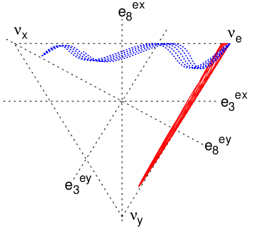
Addition of a third flavor may change the behaviour significantly, as we show in Figs. 6 and 7 for two extreme values of . We consider the case of inverted hierarchy, and a box-spectrum of energies – MeV with the number of antineutrinos as times the number of neutrinos, with . Given that the hierarchy in the solar sector is normal, we expect bipolar effect only in the subspace, combined with usual neutrino oscillations in the subspace. The following observations may be made from the figures:


- •
The evolution of both and consists of a series of bipolar “kinks” as in the two-flavor case hannestad-raffelt-sigl-wong-0608095, modulated by an envelope with the frequency . The evolutions for neutrinos and antineutrinos closely follow one another, which is expected from the conservation of .
- •
Significant three-flavor effects are present for small , since the whole triangle is seen to be filled with oscillations, forming a “petal structure” (Fig. 6). It may be interpreted as a combination of slow oscillations and bipolar oscillations that tend to take the state towards in periodic bursts.
- •
The extent of motion towards depends mainly on the asymmetry , whereas that towards depends on .
- •
For large (Fig. 7), the oscillations in the sector are suppressed since the effective mixing angle in matter becomes small. The amplitude of the bipolar motion is however not affected substantially.
Bipolar oscillations (even in the two-flavor limit) do not have a sinusoidal form, hence they are not associated with a fixed frequency. They may be looked upon as a combination of a low frequency (during the time that the component is stationary, which we shall call the A phase) and a high frequency (the sudden dip towards , which we shall call the B phase). Therefore, our prescription in Sec. II.6 has to be applied with care. Note that the order of evolution matrices in Eq. (II.6) is supposed to be in the decreasing order of frequencies. Even if we neglect the slow evolution due to , strictly speaking during the A phase, one should use the order and during the B phase, the order should be . However, we find numerically that the evolution closely matches the three-flavor solution over the complete evolution. This therefore may be taken to be the heuristic solution for the bipolar oscillations in the three-flavor case.
We have not considered normal hierarchy, in which we expect that starting with we’ll have a stable system that will not undergo bipolar oscillations, whereas starting with or , we’ll have independent bipolar oscillations towards . It will be interesting to analyze the details of such a scenario, however it is beyond the scope of this paper.
III.4 Spectral splitting
As a system of neutrinos and antineutrinos transits from the collective regime () to vacuum (), the polarization vectors keep trying to align with in the adiabatic approximation. Due to the conservation of , as shown in Sec. III.3, this alignment is not possible for all . Indeed, neutrinos with high energy need to flip over and anti-align with (which equals in vacuum) raffelt-smirnov-0705.1830; raffelt-smirnov-0709.4641. This leads to a sharp split in the energy spectrum, with the high energy getting completely converted to the non-electron flavor and vice versa.
A crucial requirement for the splits to develop is the preparation of the sytem for the split by the generation of components of that are transverse to . Bipolar oscillations do this easily for inverted hierarchy, independent of matter effects. For normal hierarchy, in the presence of large matter effects the oscillations are suppressed, but an MSW resonance can prepare the transverse components.
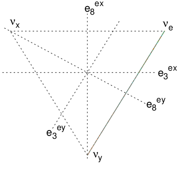
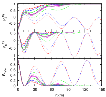
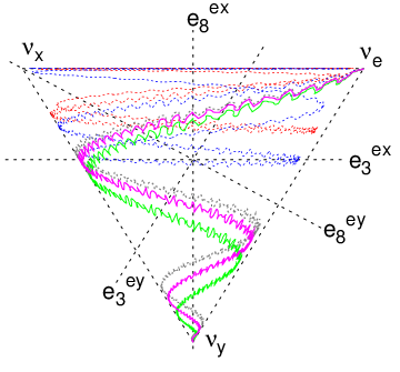
For illustration, we choose two situations, with large and small (Fig. 8 and 9 respectively) and the hierarchy is taken to be inverted. We choose the box-spectrum for and energies and the flux asymmetry . We observe the following from the figures:

- •
For large , there is only a single split for neutrinos, which can be seen in . The split is not visible in the triangle since the neutrinos are confined to the – edge. However, the low energy neutrinos move towards and the high energy ones towards .
- •
for small , the split is not only in but also in . There also are oscillations with large amplitudes. Some neutrino states drift towards and ultimately reach , while the others keep oscillating between and .
The above observations can be understood as follows. For large , the solar mixing angle is suppressed and hence the problem reduces essentially to a two-flavor one in the subspace. Thus, the split is only in . The split happens in neutrinos since there are more neutrinos than antineutrinos at any given energy. For small , in addition to the above split, there are large oscillations, which give rise to a split that is observable also in , which was absent for large .
A detailed understanding of the spectral splits in the three-flavor case, including predictions for the positions of the spectral splits has been obtained future-split.
IV Collective effects on neutrinos in SN
Collective effects are likely to be important in the context of neutrinos emitted from a SN. The number density of neutrinos and antineutrinos streaming off the neutrinosphere is quite large, so dominates over and upto a radius of a few ten or hundred kilometers respectively. Therefore, it is likely that one or more flavor conversion mechanisms identified in Sec. III come into play in the different regions inside the star.
In this section, we study the effect of collective oscillations and their interplay with subsequent MSW transitions inside a SN. To illustrate the nature of these effects, we numerically solve for the flavor evolution equations by taking a realistic SN density profile, including the collective effects. We present results primarily for inverted hierarchy, because collective effects are not expected to play a significant part for normal hierarchy 66 6 However, during the neutronization burst phase of an O-Ne-Mg SN, this need not be true.. In the numerical study, we take eV, , , and two representative values of , viz. and . We then apply the formalism developed in Sec. II to the case of neutrinos streaming from the SN neutrinosphere and identify the regimes where different flavor conversion mechanisms are at work. This allows us to explain the features in the observable neutrino and antineutrino spectra, and understand the three-flavor effects.
IV.1 SN model and parameters for numerical simulation
The SN model is defined by the following choice for the emission geometry, initial flavor dependent spectra and fluxes, the collective potential and the matter density profile. We would like to emphasize that these choices are canonical and more importantly, the specific value of the luminosity or the spatial dependence of the collective potential does not affect results significantly. Any large initial value of (such that it exceeds ) and its slow decrease with gives almost identical results. In other words, the results are not fine-tuned. However, the results would depend on the flavor spectra and the matter density profile, as these determine the initial conditions, the collective potential and the effective mixing parameters.
IV.1.1 Emission geometry
Neutrinos with different energies and flavors start freestreaming at different , but flavor evolution does not start until much later. Thus the radius of the neutrinosphere is used only to set the initial conditions. We therefore use the “bulb-model” of neutrino emission from the SN as discussed in duan-fuller-carlson-qian-0606616 with a nominal neutrinosphere at . We assume steady-state half-isotropic emission from the neutrinosphere.
IV.1.2 Initial spectra and fluxes
The flavor-dependent primary neutrino spectra at are parametrized as keil
| (150) |
where . This spectrum is normalized such that and has the average energy . The above parametrization has the advantage that the spectra can be analytically integrated, including the effects of spectral pinching through . The number flux is given by , where is the luminosity in the flavor . We remark that an equipartition in the luminosity is often assumed for simplicity. For illustration, we choose the above parameters as
| (151) |
Remembering that , we can rewrite the above information in terms of , if desired. Combining Eq. (81) with the definitions of moments in (96), allows us to calculate the values of and for the above spectrum as
| (152) | |||||
| (153) | |||||
| (154) |
Using the above expressions, is calculated to be
| (155) |
which allows us to write and in terms of , as per Eq. (142).
IV.1.3 Collective potential and matter density profile
The collective potential for for the choice of parameters in Eq. (151) is given by
| (156) |
where is given in Eq. (35). For illustration, we choose the shock-wave simulation inspired density profile that corresponds to 77 7 This is the same as the one used in fogli-lisi-mirizzi-montanino-0304056 at t=4 sec.
| (157) |
The profiles of and are shown in Fig. 10.

IV.2 Flavor conversions inside a supernova
In this section we solve for the evolution of the neutrino density matrix numerically for the chosen density profile, and show the neutrino flavor conversions. We expect synchronized oscillations in the region where km-1 fogli-lisi-marrone-mirizzi-0707.1998, which corresponds to km in our example. In the further region till km-1 fogli-lisi-marrone-mirizzi-0707.1998, which corresponds to km, bipolar oscillations are expected. Beyond this region the spectral split in the sector should develop, and subsequently MSW resonances should take place. Similarly we calculate for the flavors, the relevant values of km and km for approximate boundaries of synchronized and bipolar oscillations in the sector. However, no bipolar oscillations take place in the sector since the corresponding hierarchy is normal. In Fig. 10, we show the positions corresponding to and .
IV.2.1 Small
Fig. 11 shows the flavor evolutions in terms of and the – triangle for neutrinos as well as antineutrinos, for . This small value of ensures that the MSW resonance in antineutrinos is nonadiabatic, so that the effects of this resonance are not felt. One can then cleanly identify the collective effects. We make the following observations and interpretations based on the figure:


- •
All the neutrinos and antineutrinos initially lie on a line passing through in the – triangle. This is because the initial conditions are taken to be symmetric in and .
- •
The flavor evolution starts only at km, which is slightly beyond . Before this point, the oscillations are synchronized, with a vanishing amplitude since .
- •
Between and km, bipolar oscillations are observed as rapid dips in , and consequently in . These oscillations vanish when .
- •
Around km, a spectral split develops in neutrinos along . The spectral split tends to keep the low energy neutrinos at their original position, while taking the high energy neutrinos as well as almost all antineutrinos towards . 88 8 There seems to be a spectral split in antineutrinos as well, at very low energies. This is similar to the observation in fogli-lisi-marrone-mirizzi-0707.1998, and may be the effect of nonadiabaticity in the splitting.
- •
Between km, antineutrinos of different energies undergo the resonance. However the resonance is highly nonadiabatic and does not cause any flavor conversion.
- •
At km and beyond, the effects of the MSW resonance come into play, resulting in conversion. Since the high energy neutrinos are already close to , there is effectively no flavor conversion. However the low energy neutrinos tend to convert to , which is seen as a movement parallel to the – edge in the – triangle.
- •
Since all the flavor conversions can be understood as a net effect of two-flavor phenomena taking place in well-separated regions in the star, the flavor transitions in the – triangle are always parallel to the – edge or – edge.
Thus, for a small , the collective effects can be clearly identified, whereas the effects due to the resonance are absent. We calculate the flavor evolution till km. The collective effects have almost vanished by this time. Further MSW resonances due to the shock wave schirato-fuller-0205390; takahashi-sato-dalhed-wilson-0212195; fogli-lisi-mirizzi-montanino-0304056; tomas-kachelreiss-raffelt-dighe-janka-scheck-0407132; fogli-lisi-mirizzi-montanino-0412046; huber; dasgupta-dighe-0510219, as well as possible effects of stochastic density fluctuations or turbulence fogli-lisi-mirizzi-montanino-0603033; choubey-harries-ross-0605255; friedland-gruzinov-0607244 will govern flavor conversions here onwards. Our calculations thus provide initial conditions for neutrino spectra at this point.


In Fig. 12, we show the neutrino and antineutrino spectra at km. We see that with MeV convert almost completely to due to the spectral split, whereas lower energy convert partially to at the resonance. In the antineutrino sector, the and spectra are almost all completely swapped due to the spectral split, while the spectrum remains unaffected.


IV.2.2 Large
At large values, the resonance at – km is adiabatic, and causes significant flavor conversions in antineutrinos. In Fig. 13, we show the flavor evolution for . While the signatures of synchronized and bipolar oscillations as well as the spectral split remain identical to the case, the resonance can be seen to change the antineutrino picture substantially. The conversions in the neutrino sector, on the other hand, are identical to the small case. The following observations can be made from the figure.
- •
The spectral split gives rise to a complete – conversion, which takes antineutrinos to .
- •
The resonance again swaps the – spectra, thus undoing the earlier effect of the spectral split. This takes the antineutrinos back to their starting position in the triangle.
- •
Antineutrinos are now not on the line as in the small case. As a result, the large value of causes substantial – conversion as the neutrinos emerge from the resonance region.


The neutrino and antineutrino spectra at km are shown in Fig. 14. We see that the neutrino spectra have the same characteristics as for small . In the antineutrino sector, complete – spectral split and the reconversion at the resonance cancel each other, whereas the large value of partially mixes the – spectra.
The value of thus affects the spectra substantially. At larger values, where the resonance is more adiabatic, the spectrum is softer. The spectrum is also affected at large , as opposed to the small case.
IV.2.3 Summarized results
It is thus clear that the neutrino fluxes that reach Earth from a SN, are very different from the primary fluxes. In particular for inverted hierarchy, we learn that the and spectra are exchanged above a certain split-energy due to collective effects. For antineutrinos the swap occurs over the complete spectrum. In the normal hierarchy, collective effects do not have a significant effect. The MSW conversions cause further flavor conversions, and while the conversion probabilities have not changed from the traditional expectation, the primary fluxes entering the resonances are now vastly different. This leads to different flavor composition of the fluxes of neutrinos and antineutrinos arriving on Earth, than was traditionally expected. These fluxes can be calculated using our understanding of collective effects and the level-crossing diagrams. At the detectors on Earth one is typically sensitive to the and/or flux, and so we summarize the expectations for these fluxes in Table 1. The expressions in the table are able to describe all the features of and spectra in Figs. 12 and 14.
| Normal hierarchy | Inverted hierarchy | |
|---|---|---|
We have taken the resonance to be adiabatic. In the case of multiple resonances, as may occur during the shock wave propagation or turbulence, may be taken to be the effective jump probability (it may have a nontrivial dependence on energy and time). Note that Earth matter effects are present only when is a nontrivial combination of and .
V Conclusions
We have developed a formalism to analyze neutrino flavor conversion effects in the full three-flavor framework. It employs the Bloch vector representation for density matrices, and naturally generalizes the spin-precession analogy to three flavors. In particular, it is capable of describing three-flavor collective neutrino conversion effects inside a core collapse supernova, like synchronized oscillations, bipolar oscillations and spectral split, which have till now been analytically studied mostly in the two-flavor limit.
We explicitly extend the earlier two-flavor analysis of neutrino flavor conversions inside the SN, which includes neutrino-neutrino interactions, to three flavors, where we neglect the CP violation in the neutrino sector. We use the modified flavor basis , which is rotated from the flavor basis so as to get rid of the mixing angle . We also work in the steady state approximation so that there is no explicit time dependence in the density matrix, assume spherical symmetry and half-isotropic neutrino source, and employ the single-angle approximation that has been shown to be valid in the two-flavor case. This leads to the equations of a gyroscope in eight dimensions, similar to the three dimensional gyrosope equations in the two-flavor case.
In the three-flavor formalism, the density matrix is represented by an eight-dimensional Bloch vector . However, the flavor content is determined only by the two components and of after evolution. Motivated by this observation, we propose the “–” triangle diagram to represent the flavor content of any neutrino state by the projection of on the – plane, which we have termed P. This not only allows us to visualize the three-flavor transformations in a convenient way, but also allows us to quantify the extent of three-flavor effects over and above the two-flavor results.
A “heavy-light” factorization holds in the three-flavor treatment for certain initial conditions, so that the three-flavor results may be understood as the two-flavor results with modified with terms that depend on . Indeed, in certain situations, the three-flavor neutrino conversions may be factorized into three two-flavor oscillations with hierarchical frequencies. In such cases, the three-flavor conversion probabilities may be constructed from two-flavor results by considering the modulation of higher frequency modes by lower frequency modes.
We have compared our analytic results with the numerical ones for simple cases of an initial pure state, constant matter densities and no collective effects, as well as for synchronized oscillations, and have found a good agreement even when we ignore the modulation due to the lowest frequency. The additional effect of the third neutrino in these cases is limited to the excursions of the orbit of P towards , and has already been well studied (though without the Bloch vector treatment). In the absence of collective effects, though the evolution of all energies is different, the orbit of P can be seen to be an energy-independent quantity. In the synchronized case, neutrinos of all energies are seen to oscillate with a common frequency, and even undergo MSW resonances at the same matter density and with the same adiabaticity.
In the case of bipolar oscillations, the addition of the third neutrino changes the situation significantly. The analytical results are not so easy to obtain, however the numerical results for an inverted hierarchy show a “petal” pattern in the – triangle, which can be explained by the combination of bipolar oscillations and sinusoidal oscillations. The value of the MSW potential also plays an important role in determining the extent of the effect of the third flavor. This needs to be explored in more detail.
The spectral split occurs in neutrinos in the inverted hierarchy when one starts with , owing to the unstable position of the eight-dimensional gyroscope in this case. The above a certain energy, and almost all , completely convert to and respectively. There are no additional split effects from the introduction of the third flavor since the hierarchy in the solar sector is normal. This, however, could change if neutrinos are not in a pure state as they enter the bipolar region.
We have simulated the neutrino flavor conversions numerically by taking a realistic density profile for the SN, and have shown the flavor conversions for inverted hierarchy and two values in the cooling phase. In such a scenario, it is easily possible to identify regions where different collective as well as MSW effects dominate. We are able to predict the regions in which these effects take place, and our three-flavor formalism can explain the features of flavor conversions therein. We also point out an interplay between the collective and MSW effects. For example, the resonance cancels the effect of the spectral split for antineutrinos, whereas the spectral split makes the resonance irrelevant for neutrinos above the split energy. If the hierarchy were normal, the collective effects would be effectively absent in the cooling phase.
In conclusion, a complete understanding of the neutrino flavor conversions inside a SN requires a three-flavor treatment. In this paper, we have developed a formalism to handle this analytically, provided a method to estimate the three-flavor probabilities using the two-flavor results in certain situations, and have pointed out an interplay between collective and MSW effects, which can be easily understood with the formalism.
Acknowledgements
We would like to thank K. Damle, S. Gupta, R. Loganayagam, A. Mirizzi, G. G. Raffelt for useful discussions and insightful comments, and V. Tripathi for factors of three. This work is partly supported through the Partner Group program between the Max Planck Institute for Physics and Tata Institute of Fundamental Research.
Appendix A Notation
This paper uses 3-vectors, matrices, 8-vectors, their components and their projections in two-dimensional planes. We have tried to be consistent in the use of fonts for all these objects. The convention followed for indices is:
- •
index mass eigenstates
- •
index modified flavor eigenstates
- •
are SU(3) indices.
The convention followed for symbols is:
- •
Three-dimensional vectors are denoted by smallcase boldfaced letters, e.g. .
- •
matrices are denoted in the regular math mode, e.g. . Note however the exceptions, energy and the Fermi constant , that are also respresented in this font.
- •
Sets of matrices are denoted by blackboard-bold font, e.g. .
- •
Eight-dimensional vectors are written in bold capital letters, e.g. . Exceptions are , which are vectors along the coordinate axes, and therefore conventionally written in smallcase.
- •
The components of an eight-vector are written as .
- •
is a eight-dimensional vector whose components are matrices .
- •
Projections of eight-vectors on the – plane, e.g. P, as well as the rotation and evolution matrices on that plane, e.g. are written in sans-serif font.
References
- (1) G. G. Raffelt, “Supernova neutrino observations: What can we learn?,” [astro-ph/0701677].
- (2) A. Dighe, “Neutrinos from a core collapse supernova,” AIP Conf. Proc. 981 (2008) 75 arXiv:0712.4386 [hep-ph].
- (3) L. Wolfenstein,“Neutrino Oscillations In Matter,” Phys. Rev. D 17, 2369 (1978).
- (4) S. P. Mikheev and A. Yu. Smirnov, “Resonance Enhancement Of Oscillations In Matter And Solar Neutrino Spectroscopy,” Yad. Fiz. 42, 1441 (1985) [Sov. J. Nucl. Phys. 42, 913 (1985)].
- (5) G. M. Fuller, R. W. Mayle, J. R. Wilson, and D. N. Schramm “Resonant neutrino oscillations and stellar collapse,” Astrophys. J. 322 795 (1987).
- (6) A. S. Dighe and A. Y. Smirnov, “Identifying the neutrino mass spectrum from the neutrino burst from a supernova,” Phys. Rev. D 62 (2000) 033007 [hep-ph/9907423].
- (7) C. Lunardini and A. Yu. Smirnov, “Probing the neutrino mass hierarchy and the 13-mixing with supernovae,” JCAP 0306, 009 (2003) [hep-ph/0302033].
- (8) A. S. Dighe, M. T. Keil and G. G. Raffelt, “Detecting the neutrino mass hierarchy with a supernova at IceCube,” JCAP 0306, 005 (2003) [hep-ph/0303210].
- (9) A. S. Dighe, M. T. Keil and G. G. Raffelt, “Identifying earth matter effects on supernova neutrinos at a single detector,” JCAP 0306, 006 (2003) [hep-ph/0304150].
- (10) A. S. Dighe, M. Kachelriess, G. G. Raffelt and R. Tomas, “Signatures of supernova neutrino oscillations in the earth mantle and core,” JCAP 0401, 004 (2004) [hep-ph/0311172].
- (11) R. C. Schirato and G. M. Fuller, “Connection between supernova shocks, flavor transformation, and the neutrino signal,” [astro-ph/0205390].
- (12) K. Takahashi, K. Sato, H. E. Dalhed and J. R. Wilson, “Shock propagation and neutrino oscillation in supernova,” Astropart. Phys. 20, 189 (2003) [astro-ph/0212195].
- (13) G. L. Fogli, E. Lisi, A. Mirizzi, and D. Montanino, “Analysis of energy- and time-dependence of supernova shock effects on neutrino crossing probabilities,” Phys. Rev. D 68, 033005 (2003) [hep-ph/0304056].
- (14) R. Tomàs, M. Kachelrieß, G. Raffelt, A. Dighe, H. T. Janka and L. Scheck, “Neutrino signatures of supernova shock and reverse shock propagation,” JCAP 0409, 015 (2004) [astro-ph/0407132].
- (15) G. L. Fogli, E. Lisi, A. Mirizzi and D. Montanino, “Probing supernova shock waves and neutrino flavor transitions in next-generation water-Cherenkov detectors,” JCAP 0504, 002 (2005) [hep-ph/0412046].
- (16) V. Barger, P. Huber and D. Marfatia, “Supernova neutrinos can tell us the neutrino mass hierarchy independently of flux models,” Phys. Lett. B 617, 167 (2005) [hep-ph/0501184].
- (17) B. Dasgupta and A. Dighe, “Phase effects in neutrino conversions during a supernova shock wave,” Phys. Rev. D 75 (2007) 093002 [hep-ph/0510219].
- (18) G. L. Fogli, E. Lisi, A. Mirizzi and D. Montanino, “Damping of supernova neutrino transitions in stochastic shock-wave density profiles,” JCAP 0606, 012 (2006) [hep-ph/0603033].
- (19) S. Choubey, N. P. Harries and G. G. Ross, “Probing neutrino oscillations from supernovae shock waves via the IceCube detector,” Phys. Rev. D 74, 053010 (2006) [hep-ph/0605255].
- (20) A. Friedland and A. Gruzinov, “Neutrino signatures of supernova turbulence,” [astro-ph/0607244].
- (21) J. P. Kneller, G. C. McLaughlin and J. Brockman, “Oscillation Effects and Time Variation of the Supernova Neutrino Signal,” arXiv:0705.3835 [astro-ph].
- (22) J. T. Pantaleone, “Dirac neutrinos in dense matter,” Phys. Rev. D 46 510 (1992).
- (23) J. Pantaleone, “Neutrino oscillations at high densities,” Phys. Lett. B 287, 128 (1992).
- (24) M. J. Thomson and B. H. J. McKellar, “The nonlinear MSW equation,” Phys. Lett. B 259, 113 (1991).
- (25) G. Sigl and G. Raffelt, “General kinetic description of relativistic mixed neutrinos,” Nucl. Phys. B 406, 423 (1993).
- (26) B. H. J. McKellar and M. J. Thomson, “Oscillating doublet neutrinos in the early universe,” Phys. Rev. D 49, 2710 (1994).
- (27) S. Samuel, “Neutrino oscillations in dense neutrino gases,” Phys. Rev. D 48, 1462 (1993).
- (28) V. A. Kostelecký and S. Samuel, “Self-maintained coherent oscillations in dense neutrino gases,” Phys. Rev. D 52, 621 (1995) [hep-ph/9506262].
- (29) J. Pantaleone, “Stability of incoherence in an isotropic gas of oscillating neutrinos,” Phys. Rev. D 58, 073002 (1998).
- (30) S. Samuel, “Bimodal coherence in dense selfinteracting neutrino gases,” Phys. Rev. D 53, 5382 (1996) [hep-ph/9604341].
- (31) S. Pastor, G. G. Raffelt and D. V. Semikoz, “Physics of synchronized neutrino oscillations caused by self-interactions,” Phys. Rev. D 65, 053011 (2002) [hep-ph/0109035].
- (32) S. Hannestad, G. G. Raffelt, G. Sigl and Y. Y. Y. Wong, “Self-induced conversion in dense neutrino gases: Pendulum in flavour space,” Phys. Rev. D 74, 105010 (2006) [Erratum-ibid. D 76, 029901 (2007)] [astro-ph/0608695].
- (33) H. Duan, G. M. Fuller, J. Carlson and Y. Z. Qian, “Analysis of Collective Neutrino Flavor Transformation in Supernovae,” Phys. Rev. D 75, 125005 (2007) [astro-ph/0703776].
- (34) G. G. Raffelt and A. Y. Smirnov, “Self-induced spectral splits in supernova neutrino fluxes,” Phys. Rev. D 76 081301 (2007) arXiv:0705.1830 [hep-ph].
- (35) G. G. Raffelt and A. Y. Smirnov, “Adiabaticity and spectral splits in collective neutrino transformations,” arXiv:0709.4641 [hep-ph].
- (36) J. T. Pantaleone, “Neutrino flavor evolution near a supernova’s core,” Phys. Lett. B 342, 250 (1995) [astro-ph/9405008].
- (37) Y. Z. Qian and G. M. Fuller, “Neutrino-neutrino scattering and matter enhanced neutrino flavor transformation in Supernovae,” Phys. Rev. D 51, 1479 (1995) [astro-ph/9406073].
- (38) G. Sigl, “Neutrino mixing constraints and supernova nucleosynthesis,” Phys. Rev. D 51, 4035 (1995) [astro-ph/9410094].
- (39) S. Pastor and G. Raffelt, “Flavor oscillations in the supernova hot bubble region: Nonlinear effects of neutrino background,” Phys. Rev. Lett. 89, 191101 (2002) [astro-ph/0207281].
- (40) A. B. Balantekin and H. Yüksel, “Neutrino mixing and nucleosynthesis in core-collapse supernovae,” New J. Phys. 7, 51 (2005) [astro-ph/0411159].
- (41) H. Duan, G. M. Fuller, J. Carlson and Y. Z. Qian, “Simulation of coherent non-linear neutrino flavor transformation in the supernova environment. I: Correlated neutrino trajectories,” Phys. Rev. D 74, 105014 (2006) [astro-ph/0606616].
- (42) H. Duan, G. M. Fuller, J. Carlson and Y. Z. Qian, “Coherent development of neutrino flavor in the supernova environment,” Phys. Rev. Lett. 97, 241101 (2006) [astro-ph/0608050].
- (43) G. M. Fuller and Y. Z. Qian, “Simultaneous flavor transformation of neutrinos and antineutrinos with dominant potentials from neutrino neutrino forward scattering,” Phys. Rev. D 73, 023004 (2006) [astro-ph/0505240].
- (44) H. Duan, G. M. Fuller and Y. Z. Qian, “Collective neutrino flavor transformation in supernovae,” Phys. Rev. D 74, 123004 (2006) [astro-ph/0511275].
- (45) H. Duan, G. M. Fuller and Y. Z. Qian, “A Simple Picture for Neutrino Flavor Transformation in Supernovae,” Phys. Rev. D 76, 085013 (2007) arXiv:0706.4293 [astro-ph].
- (46) H. Duan, G. M. Fuller, J. Carlson and Y. Q. Zhong, “Neutrino Mass Hierarchy and Stepwise Spectral Swapping of Supernova Neutrino Flavors,” arXiv:0707.0290 [astro-ph].
- (47) A. Esteban-Pretel, S. Pastor, R. Tomàs, G. G. Raffelt and G. Sigl, “Decoherence in supernova neutrino transformations suppressed by deleptonization,” arXiv:0706.2498 [astro-ph].
- (48) G. L. Fogli, E. Lisi, A. Marrone and A. Mirizzi, “Collective neutrino flavor transitions in supernovae and the role of trajectory averaging,” arxiv:0707.1998 [hep-ph].
- (49) G. G. Raffelt and G. Sigl, “Self-induced decoherence in dense neutrino gases,” Phys. Rev. D 75, 083002 (2007) [hep-ph/0701182].
- (50) H. Duan, G. M. Fuller, J. Carlson and Y. Z. Qian, “Flavor Evolution of the Neutronization Neutrino Burst from an O-Ne-Mg Core-Collapse Supernova,” arXiv:0710.1271 [astro-ph].
- (51) V. A. Kostelecký, J. Pantaleone and S. Samuel, “Neutrino oscillation in the early universe,” Phys. Lett. B 315, 46 (1993).
- (52) V. A. Kostelecký and S. Samuel, “Neutrino oscillations in the early universe with an inverted neutrino mass hierarchy,” Phys. Lett. B 318, 127 (1993).
- (53) V. A. Kostelecký and S. Samuel, “Nonlinear neutrino oscillations in the expanding universe,” Phys. Rev. D 49, 1740 (1994).
- (54) V. A. Kostelecký and S. Samuel, “Neutrino oscillations in the early universe with nonequilibrium neutrino distributions,” Phys. Rev. D 52, 3184 (1995) [hep-ph/9507427].
- (55) V. A. Kostelecký and S. Samuel, “Nonequilibrium neutrino oscillations in the early universe with an inverted neutrino mass hierarchy,” Phys. Lett. B 385, 159 (1996) [hep-ph/9610399].
- (56) A. D. Dolgov, S. H. Hansen, S. Pastor, S. T. Petcov, G. G. Raffelt and D. V. Semikoz, “Cosmological bounds on neutrino degeneracy improved by flavor oscillations,” Nucl. Phys. B 632 363 (2002) [hep-ph/0201287].
- (57) Y. Y. Y. Wong, “Analytical treatment of neutrino asymmetry equilibration from flavour oscillations in the early universe,” Phys. Rev. D 66, 025015 (2002) [hep-ph/0203180].
- (58) Y. Y. Y. Wong, “Synchronised neutrino oscillations from self interaction and associated applications,” AIP Conf. Proc. 655, 240 (2003) [hep-ph/0211045].
- (59) K. N. Abazajian, J. F. Beacom and N. F. Bell, “Stringent constraints on cosmological neutrino antineutrino asymmetries from synchronized flavor transformation,” Phys. Rev. D 66, 013008 (2002) [astro-ph/0203442].
- (60) A. Esteban-Pretel, S. Pastor, R. Tomas, G. G. Raffelt and G. Sigl, “Mu-tau neutrino refraction and collective three-flavor transformations in supernovae,” arXiv:0712.1137 [astro-ph].
- (61) C. Y. Cardall, “Liouville equations for neutrino distribution matrices,” arXiv:0712.1188 [astro-ph].
- (62) G. Kimura, “The Bloch Vector for N-Level Systems,” Phys. Lett. A 314, 339 (2003) [quant-ph/0301152].
- (63) C. W. Kim, J. Kim and W. K. Sze, “Geometrical representation of neutrino oscillations in vacuum and matter,” Phys. Rev. D 37, 1072 (1988).
- (64) B. Dasgupta, A. Dighe, A. Mirizzi and G. G. Raffelt, “Spectral split in prompt supernova neutrino burst: Analytic three-flavor treatment,” arXiv:0801.1660 [hep-ph].
- (65) M. T. Keil, G. G. Raffelt and H. T. Janka, “Monte Carlo study of supernova neutrino spectra formation,” Astrophys. J. 590, 971 (2003) [astro-ph/0208035].