Collinear Singularities and Running Coupling
Corrections to Gluon Production in CGC

In the recent years there has been a lot of progress in understanding running coupling corrections for small-$x$ evolution equations. Running coupling corrections to the Balitsky-Fadin-Kuraev-Lipatov (BFKL) [1, 2], the Balitsky-Kovchegov (BK) [3, 4, 5, 6, 7] and the Jalilian-Marian–Iancu–McLerran–Weigert–Leonidov–Kovner (JIMWLK) [8, 9, 10, 11, 12, 13, 14, 15] evolution equations were calculated in [16, 17, 18, 19]. Knowledge of the running coupling corrections to the BK and JIMWLK equations significantly improved our ability to make precise predictions for the total cross sections in deep inelastic scattering (DIS) based on the saturation/Color Glass Condensate (CGC) physics [20, 21, 22, 23, 24, 25, 26, 27, 8, 9, 10, 11, 12, 13, 14, 15, 6, 7, 3, 4, 5, 28, 29, 30].

However, to improve the CGC predictions for other observables, such as the inclusive gluon or quark production cross sections, it is important to understand how the running coupling corrections enter the expressions derived previously for such cross sections [31, 32, 33, 34, 35, 36, 37, 38, 39, 40, 41, 42, 43, 44, 45, 46, 47]. It was originally proposed in [20, 48] that the gluon production cross section can be described by the $k_{T}$-factorization formula

$\displaystyle\frac{d\sigma}{d^{2}p\,dy}\,=\,\frac{2\,\alpha_{s}}{C_{F}}\,\frac{1}{p_{T}^{2}}\,\int d^{2}q\,\phi_{p}({\bm{q}},y)\,\phi_{t}({\bm{p}}-{\bm{q}},Y-y),$

(1)

where the gluon is produced with the transverse momentum $\bm{p}$ ($p_{T}=|{\bm{p}}|$), rapidity $y$ in a collision with the total rapidity interval $Y$. $\phi_{p}$ and $\phi_{t}$ are the unintegrated gluon distribution functions in the projectile and in the target correspondingly. $\alpha_{s}$ is the strong coupling constant and $C_{F}=(N_{c}^{2}-1)/2N_{c}$.

$k_{T}$-factorization (1) has been known to work outside the saturation region [49, 31, 32, 33, 34] (e.g. for proton-proton collisions $pp$). In [38, 50, 41] it was shown that the $k_{T}$-factorization formula (1) holds for gluon production in proton-nucleus ($pA$) collisions and in DIS both in the quasi-classical limit of multiple rescatterings [22, 23, 24, 25] and after including quantum BK/JIMWLK evolution. This means that Eq. (1) works in the kinematic region inside the saturation region for the target and outside the saturation region for the projectile. (A proton/projectile can be defined as a nucleus with a much smaller saturation scale than in the target nucleus.) It is at present not clear whether Eq. (1) correctly describes gluon production in nucleus-nucleus collisions, i.e., in the saturation region for both the target and the projectile.

In [38] the following relation was also derived between the forward amplitude of a dipole of transverse size $\bm{x}$ scattering on a nucleus at impact parameter $\bm{b}$ and rapidity $y$, $N({\bm{x}},{\bm{b}},y)$, and the unintegrated gluon distribution function $\phi({\bm{q}},y)$ of the same nucleus:

$\displaystyle\phi({\bm{q}},y)\,=\,\frac{C_{F}}{\alpha_{s}\,(2\,\pi)^{3}}\,\int d^{2}b\,d^{2}x\,e^{-i{\bm{q}}\cdot{\bm{x}}}\,\nabla^{2}_{x}\,N({\bm{x}},{\bm{b}},y).$

(2)

It would be very interesting to see if Eq. (1) would still hold when running coupling corrections are included. It would also be interesting to see whether the relation (2) would survive the inclusion of running coupling corrections. This would verify the validity of $k_{T}$-factorization formula (1) and the universality of the dipole amplitude as the correct degree of freedom for both the total DIS cross section and for the single gluon production at small-$x$.

To answer the above questions one has to first understand how to include running coupling corrections into the gluon production cross section. This is a formidable task that we are not going to complete here. Instead we will be content with a first step in that direction by resolving some conceptual questions and by setting up a formalism for future calculations. Our main task is to identify the cancellation mechanisms that ensure the IR safety of the total cross section, as it governs all left over phase space cancellations for less inclusive observables and allows us to pinpoint the origin of eventual IR problems.

Below we will analyze the running coupling corrections to the one-gluon inclusive production cross section. Our strategy is standard: following Brodsky, Lepage and Mackenzie (BLM) [51] we will begin by dressing all the relevant gluon lines and vertices by quark bubble chains, resumming powers of $\alpha_{s}\,N_{f}$. We will then replace

$\displaystyle N_{f}\rightarrow-6\,\pi\,\beta_{2}$

(3)

to complete it to the full one-loop QCD beta-function

$\displaystyle\beta_{2}=\frac{11N_{c}-2N_{f}}{12\,\pi}.$

(4)

Resumming all factors of $\alpha_{\mu}\,\beta_{2}$ should replace all factors of the bare coupling constant $\alpha_{\mu}$ in the original lowest order expression (1) by the physical couplings.¹¹ 1 We refer the reader to  [52, 53, 54, 55] and [56, 57, 58] for a discussion of the context and validity the BLM resummation procedure or its refinements, for example via the dispersive method. The first issue here is whether the quark bubbles faithfully trace all running coupling corrections and thus justify (3): The answer given in the references is that this is true in the “single dressed gluon approximation,” i.e. if the process only involves one gluon line that needs to be dressed. The second issue is the all orders resummation involved in renormalizing the coupling: This is deeply connected with the large order behavior of perturbation theory and the notion of renormalons [59, 60]. Despite the natural quantitative uncertainties inherent in trying to answer the question of what is the scale in the coupling, the BLM method should at least yield a qualitatively correct answer and most importantly, be able to tell perturbative from non-perturbative contributions. If one takes the most conservative and pessimistic view, one can always reexpand the resummed coupling back to its lowest scale carrying order and estimate the uncertainty induced by varying the renormalization scale $\mu$ “within reasonable bounds.” Our expressions must match these lowest order corrections as exemplified for the running coupling corrections to the non-linear small-$x$ evolution in the calculation of the gluonic component of the NLO BFKL, BK, and JIMWLK kernels done in [61]. In [61] the result of a full NLO calculation confirmed the scale-setting for the running coupling which had been done in [16, 17] using the BLM prescription.

The paper is structured as follows. In Sect. 2 we will set up the formalism for including quark bubbles in the final state (the state after the projectile’s interaction with the target). We will then analyze the running coupling corrections to gluon production in Sect. 3.

The main conceptual problem in including running coupling corrections for the gluon production cross section is with insertion of quark bubbles onto the outgoing gluon line (see Fig. 11 below). Indeed, if one uses dimensional regularization and the quarks are massless all such bubble corrections are zero, since the on-mass-shell gluon provides no invariant momentum scale. This zero can be thought about as a “cancellation” of the infrared and ultraviolet divergences in the bubbles. The zero result is unsatisfactory, since it would leave the gluon production cross section proportional to a factor $\alpha_{\mu}$, the bare coupling, and thus unrenormalized.

To resolve this problem we notice that collinear divergences, resulting from gluon splitting into two massless quarks (or gluons) come in at the same order in perturbation theory as running coupling corrections on the outgoing gluon line. To keep track of such divergences we regularize them with the infrared cutoff $\Lambda_{\text{coll}}$. With the regulator inserted, we show in Sect. 3 that the bubbles on the outgoing gluon line generate a factor of running coupling $\alpha_{s}(\Lambda_{\text{coll}}^{2})$ with the infrared (IR) cutoff in the argument. Therefore, the gluon production cross section has to come in with a factor of the coupling running with some arbitrary IR cutoff in the argument. Indeed the cutoff has a meaning of the resolution scale for gluons: once such a cutoff is introduced, collinear $q\bar{q}$ pairs (and collinear gluon pairs) are also identified as gluons, generating extra diagrams contributing running coupling corrections (see Fig. 13), which in the end renormalize gluon production cross section. We conclude that the gluon production cross section depends on the IR cutoff/resolution scale and is thus not infrared-safe, in agreement with conventional wisdom.

Our argument shows that the result of the full calculation of the running coupling corrections would necessarily generate a power of $\alpha_{s}(\Lambda_{\text{coll}}^{2})$. We expect that, again in line with conventional wisdom, such non-perturbative factors of the coupling could be absorbed into fragmentation functions if hadron production is the goal of a calculation at hand. The separation of the diagrams into the perturbative cross sections and the fragmentation functions could be done using the conventional approach (see e.g. [62, 63] and references therein). It would result in a factorization scale dependence for both the perturbative cross section and the fragmentation function.

Indeed one might worry that when Eq. (1) is applied to $pA$ collisions, the unintegrated gluon distribution in the projectile proton $\phi_{p}$ would depend on some non-perturbative scale $\Lambda$ characterizing the proton, thus making the gluon production cross section in Eq. (1) non-perturbative even without the inclusion of running coupling corrections. This is a legitimate concern, though, for instance, it does not apply to the case of DIS, where the scale characterizing the projectile is the photon’s virtuality $Q^{2}\gg\Lambda_{\text{QCD}}^{2}$, which makes both $\phi_{p}$ and the cross section in Eq. (1) perturbative before the inclusion of running coupling corrections. However, even in the case of DIS, running coupling corrections would still lead to the collinear singularities that we discuss below, making the gluon production cross section not infrared-safe. The problem of applying Eq. (1) to $pA$ collisions is expected to be remedied in nucleus-nucleus ($AA$) collisions or in $pA$ collisions at very high energies, where the IR-safety of the gluon production cross section at fixed coupling is expected to be imposed by the saturation effects in both the target and the projectile (see [31, 32, 33, 34]). While we can not prove that here, we also expect the collinear singularities discussed below to arise if one tries to calculate the running coupling corrections to the gluon production in $AA$ collisions.

We continue our discussion by examining an observable built from quark and gluon production cross sections which is infrared-safe in Sect. 4. The goal is to show explicitly how the infrared contributions cancel to render the quantity infrared-safe. The observable is the energy density of the matter produced in a collision. In [64] the energy density of the medium produced in a heavy ion collision at the space-time point described by the proper time $\tau$, space-time rapidity $\eta$ and transverse coordinate ${\bm{b}}=(b_{1},b_{2})$ was shown to be given by the following formula:

$\displaystyle\epsilon(\tau,\eta,{\bm{b}})\,=\,\frac{1}{\tau}\,\int d^{2}p\,p_{T}\,\left\{\frac{dN^{G}}{d^{2}p\,d\eta\,d^{2}b}+\frac{dN^{q}}{d^{2}p\,d\eta\,d^{2}b}+\frac{dN^{\bar{q}}}{d^{2}p\,d\eta\,d^{2}b}\right\}.$

(5)

Here $\frac{dN^{G}}{d^{2}p\,dy\,d^{2}b}$ is the number of gluons produced with transverse momentum $\bm{p}$, momentum-space rapidity $y$ and at transverse coordinate $\bm{b}$. The quark and anti-quark production contributions $\frac{dN^{q}}{d^{2}p\,d\eta\,d^{2}b}$ and $\frac{dN^{\bar{q}}}{d^{2}p\,d\eta\,d^{2}b}$ are added to the gluon one on the right hand side of Eq. (5). Note that the momentum space rapidity $y$ gets replaced by the space-time rapidity $\eta$ in Eq. (5). The above formula (5) is valid for sufficiently late proper times, $\tau\gg 1/\langle p_{T}\rangle$ with $\langle p_{T}\rangle$ the typical transverse momentum of the produced quarks and gluons. The corrections to it are suppressed by extra powers of $\tau$ [64]. Eq. (5), along with our discussion below, is applicable to the particles produced at central rapidity, i.e., particles with small-$x$ both in the target and the projectile wave functions. Eq. (5) is valid not only for heavy ion collisions, but for $pp$, $pA$ and DIS collisions as well.

In Sect. 4 we show that the energy density (5) is indeed independent of the IR cutoff $\Lambda_{\text{coll}}$ by showing that terms in the gluon (and quark) multiplicity which depend of this cutoff and which are singular in the $\Lambda_{\text{coll}}\rightarrow 0$ limit actually vanish when inserted in Eq. (5) using the abstract structure of the equation. In Sect. 5 we demonstrate how these terms vanish in an explicit toy model: we show that collinearly divergent terms have such a $p_{T}$-dependence, that, when inserted in Eq. (5), they integrate out to zero. Thus energy density is an infrared-finite quantity.

We also argue that the running coupling corrections are included in the expression for the energy density (5) in a manner similar to the total cross section calculation [16, 17, 18, 19], since both gluons and quarks are allowed in the final state for either the total cross section or for the energy density.

As an aside we discuss the renormalization of the interaction of the projectile wave function with the target in Appendix A using a quark-antiquark dipole as the projectile. We find how the running coupling corrections enter the Glauber-Mueller formula (A1) [65]. We obtain that one of the two couplings in the exponent of Eq. (A1) runs with the inverse transverse size of the dipole, while the other coupling runs with some non-perturbative scale characterizing nucleons in the nucleus, as shown in Eq. (A8).

We conclude in Sect. 6 by discussing our main results and potential future developments.

We begin by analyzing the running coupling corrections to the total cross section arising in the final state. Our discussion will apply to both the cross sections calculated in the quasi-classical approximation of McLerran-Venugopalan (MV) model [24, 23, 22] and to the cross sections where the corrections due to non-linear small-$x$ evolution equations [3, 4, 5, 6, 7, 8, 9, 10, 11, 12, 13, 14, 15] are included. Just like in the calculation of the total dipole-nucleus cross section, the corrections due to small-$x$ evolution come in through a sequence of longitudinally soft gluon emissions, as only gluonic corrections generate leading logarithms of Bjorken $x$ (i.e. powers of $\alpha_{s}\,\ln 1/x$) [1, 2]. Our discussion below can equally be applied to the quasi-classical gluon production in the MV model, or to the gluon production enhanced by small-$x$ evolution corrections, which appears as a quasi-classical gluon emission in one rung of the small-$x$ evolution (see e.g. [38, 30]). Common to both cases is an eikonal emission vertex for the gluons under consideration.

In [17, 16, 18, 66] the running coupling corrections to the non-linear small-$x$ evolution equations [6, 7, 3, 4, 5, 27, 8, 9, 10, 11, 12, 13, 14, 15] were calculated for the first time. The BK and JIMWLK evolution equations were written for the total cross section of a projectile (dipole) scattering on a target: therefore the optical theorem is applicable and allows to neglect all the final state interactions. This was used in [17, 18] to specifically discard the final state running coupling corrections. In [16] one-loop final state corrections were studied at order $\alpha_{s}\,N_{f}$ and their cancellation was shown explicitly at that level. While we indeed expect also the all orders resummed final state fermion bubble insertions to cancel due to the optical theorem, we expect the explicit mechanism of this cancellation to be far from straightforward. Thus we set out to explore how the cancellation works explicitly.

Before we begin, let us introduce the notations. We will consider a high energy proton-nucleus or DIS collision and will work in the center of mass frame. In this frame the incoming proton/$q\bar{q}$ dipole (henceforth referred to as the projectile) comes in from the light cone time of $x_{+}=-\infty$ moving along the $x_{+}$-axis. The wave function of the projectile may contain extra gluonic fluctuations. The projectile scatters on the target instantaneously at the light cone time $x_{+}=0$. Similar to [38, 67, 40] we will denote the instantaneous interaction with the target by a broad (blue) vertical line, as shown in Fig. 1. The broad (blue) line comprises all possible multiple one- and two-gluon exchanges between the nucleons in the target and the projectile (similar to Fig. 15 in the Appendix A). These interactions of the target field with projectile constituents or the emitted gluon shown explicitly sum into path ordered exponentials along the projectile light cone direction. They are indicated for the emitted gluon (or any explicitly shown interacting quark in what is to follow) in form of an oval (red) mark. After scattering on the target the system evolves further towards the final state at light cone time $x_{+}=+\infty$. This final state we will denote by a vertical solid line as shown in Fig. 1 and refer to it as the final state cut, as appropriate when talking about diagrammatic contributions to probabilities instead of amplitudes.

The amplitude squared, using a similar notation, is shown in the center of Fig. 2.

There the light cone time goes from $x_{+}=-\infty$ to $x_{+}=+\infty$ both in the amplitude and in its complex conjugate. In the case of the projectile dipole one has to sum over all possible emissions of the gluon by the quark and the anti-quark, both in the amplitude and in the complex conjugate amplitude. In case of the proton projectile the emissions off all of the valence quarks have to be resummed. To save space we will introduce an abbreviated notation, shown on the right hand side of Fig. 2. The disconnected gluon line implies sum over emissions of the gluon by all quarks in the projectile. The broad (blue) line indicates all multiple rescatterings in the amplitude. This notation also makes it easier to discuss our results in relation to any type of (small) projectile.

In the notation of the graph on the right of Fig. 2 the optical theorem can be formulated as follows: to calculate the total scattering cross section the dynamics between $x_{+}=0$ and $x_{+}=+\infty$ can be ignored. For instance, if we wanted to find contribution of extra softer gluon emissions to the total cross section, only emissions at light cone time $-\infty<x_{+}<0$ should be included both in the amplitude and in the complex conjugate amplitude. This indeed has been verified in the literature [68, 38]. The same property applies to running coupling corrections. The quark bubbles dressing the gluon line at times $0<x_{+}<+\infty$ do not contribute to the total cross section according to the optical theorem. Such corrections were indeed not included in the calculations of [17, 16, 18, 66]. However, these corrections should be included if one is interested in gluon production cross section. To learn how to best organize a calculation that includes them, we will first see how they cancel in the total cross section.

To set the stage, let us briefly recall how the cancellations for the cross section mandated by the optical theorem work at leading order. The diagrams to consider for the amplitude include all contributions from order $g^{0}$ through $g^{2}$:

$\displaystyle\parbox{56.9055pt}{\includegraphics[width]{order-0-amp}}+\parbox{56.9055pt}{\includegraphics[width]{order-g-initial}}+\parbox{56.9055pt}{\includegraphics[width]{order-g-final}}+\parbox{56.9055pt}{\includegraphics[width]{order-g2_virt_initial}}+\parbox{56.9055pt}{\includegraphics[width]{order-g2_virt_interact}}+\parbox{56.9055pt}{\includegraphics[width]{order-g2_virt_final}}$

(6)

The optical theorem guarantees that at order $\alpha_{s}$, the only diagrams contributing to the absolute value squared of this amplitude are

$\displaystyle\parbox{113.81102pt}{\includegraphics[height]{oc_v_l}}+\parbox{113.81102pt}{\includegraphics[height]{oc_real}}+\parbox{113.81102pt}{\includegraphics[height]{oc_v_r}}\ .$

(7)

This quite drastic reduction in the number of diagrams one needs to calculate to obtain the total cross section is due to the following set of separate cancellations:

	$\displaystyle\parbox{113.81102pt}{\includegraphics[height]{oc_lc_1}}+\parbox{113.81102pt}{\includegraphics[height]{oc_lc_2}}\hskip 5.12149pt\phantom{+\parbox{113.81102pt}{\includegraphics[height]{oc_lc_2}}}=$	$\displaystyle\ 0$		(8a)
	$\displaystyle\parbox{113.81102pt}{\includegraphics[height]{oc_mc_1}}+\parbox{113.81102pt}{\includegraphics[height]{oc_mc_2}}+\parbox{113.81102pt}{\includegraphics[height]{oc_mc_3}}=$	$\displaystyle\ 0$		(8b)
	$\displaystyle\phantom{\parbox{113.81102pt}{\includegraphics[height]{oc_mc_1}}+}\parbox{113.81102pt}{\includegraphics[height]{oc_rc_1}}+\parbox{113.81102pt}{\includegraphics[height]{oc_rc_2}}=$	$\displaystyle\ 0\ .$		(8c)

That the cancellation pattern is separated out into three groups is dictated by the interaction of the produced gluon with the target as marked by the (red) dot on the interaction area: only diagrams with identical interaction patterns can possibly cancel against each other. This will be the first guiding principle to identify potential cancellations below. The actual cancellations require further analysis of the integrals associated with the diagrams. If one restricts the sum over the final state phase space, the cancellations are no longer complete. Still, partial cancellations from the phase space regions that have not been excluded from the final state sum remain in effect and only become manifest if one groups the diagrams as shown in (8).

We will not analyze all contributions exhaustively but rather focus on a number of subsets of the one and two loop fermion bubble insertions that cancel separately in the total cross section to illustrate and identify the basic mechanisms at work. This will lay the groundwork to allow us to precisely pinpoint the origin of IR divergences, understand how they cancel in the total cross section. It also allows to understand, for example, the cancellations of UV logarithms of the form $\ln(s/\mu)$ present in individual diagrams (with $\mu$ the renormalization scale, a UV quantity) from the final result. All these relationships are a prerequisite for a full calculation of the running coupling corrections that remains beyond the scope of the present paper.

We begin with a single fermion bubble. The relevant diagrams with final state interactions (splittings and mergers) are shown in Figs. 3 and 4.

Due to light-cone time-ordered nature of these graphs, it is more convenient to use light-cone perturbation theory (LCPT) rules [69, 70] to calculate them. To understand the cancellations we will concentrate almost solely on the energy denominators: apart from complex conjugation on the right hand side of the cut, the numerators of all diagrams in Fig. 3 are the same. At the same time direct application of the rules of LCPT as stated in [69, 70] appears problematic due to singularities in some of the energy denominators. One of the singular denominators corresponds to the intermediate state $\alpha$ shown in graph A in Fig. 3. The light cone energy of the state $\alpha$ is identical to that of the final (outgoing) state, generating a $1/0$-type singularity coming from the corresponding energy denominator. This problem has been discussed before in [68] for small-$x$ evolution, and our discussion here will follow the calculations performed in [68]. To tackle the problem of singularities one has to calculate the energy denominators in the diagram in Fig. 3A starting from the usual Feynman perturbation theory.

In going from Feynman perturbation theory to LCPT one performs integration over the minus components of the internal momenta in the diagram. A Fourier transform of a denominator of a gluon or quark propagator becomes

$\displaystyle\int\frac{d^{4}k}{(2\pi)^{4}}\,\frac{-i}{k^{2}+i\epsilon}\,e^{-ik\cdot x}\,=\,\int\frac{d^{2}k\,dk_{+}}{(2\pi)^{3}\,2k_{+}}\,e^{-i\left(k_{+}x_{-}+\frac{{\bm{k}}^{2}-i\epsilon}{2\,k_{+}}x_{+}-{\bm{k}}\cdot{\bm{x}}\right)}\,\left[-\theta(x_{+})\,\theta(k_{+})+\theta(-x_{+})\,\theta(-k_{+})\right]$

(9)

which effectively puts the particle on mass-shell assigning the light-cone energy (the minus component of the momentum) to be equal to

$\displaystyle E_{k}\,=\,\frac{{\bm{k}}^{2}}{2\,k_{+}}.$

(10)

Thus a particle propagating over a light cone time interval $x_{+}$ brings in a factor of

$\displaystyle e^{-iE_{k}\,x_{+}}.$

(11)

The incoming particle with momentum $(k_{+},{\bm{k}})$ brings in a factor of

$\displaystyle e^{-iE_{k}\,x_{+}}$

(12)

while the outgoing particle with momentum $(k_{+},{\bm{k}})$ brings in

$\displaystyle e^{iE_{k}\,x_{+}},$

(13)

as can be inferred from Eq. (9).

With the above rules in mind, the relevant contribution of the diagram $A$ in Fig. 3 is

$\displaystyle A\,=\,-\int\limits_{0}^{+\infty}dx_{2+}\,\int\limits_{0}^{x_{2+}}dx_{1+}\,e^{-\delta x_{1+}-\delta x_{2+}-i(x_{2+}-x_{1+})(E_{k_{1}}+E_{k_{2}})-ix_{1+}E_{q}+ix_{2+}E_{q}},$

(14)

where the overall minus sign comes from taking into account two powers of $i$ coming from the quark-gluon vertices. The omitted (numerator) part of the diagram $A$ is the same for all three graphs in Fig. 3: the gluon in all three cases can only have transverse polarizations. In Eq. (14) we have introduced light-cone regulators $\delta>0$, which make the integrals convergent at infinite light cone time. (Indeed, for the initial state emissions the regulators should come in with the opposite sign in the exponent.) The notations used in Eq. (14) are explained in Fig. 3A: the quark and anti-quark lines carry momenta $(k_{1+},{\bm{k}}_{1})$ and $(k_{2+},{\bm{k}}_{2})$ correspondingly, while the gluon carries momentum $(q_{+},{\bm{q}})=(k_{1+},{\bm{k}}_{1})+(k_{2+},{\bm{k}}_{2})$. The quark-gluon vertices are assigned light cone times $x_{1+}$ and $x_{2+}$, as shown in Fig. 3A. Due to theta-functions in Eq. (9) one can see that only the ordering $0\leq x_{1+}\leq x_{2+}<+\infty$ used in Eq. (14) is allowed, as $q_{+}>0$ for the produced gluon.

Performing the integrations in Eq. (14) and expanding the result in the powers of $\delta$ yields

$\displaystyle A\,=\,-\frac{i}{2\,\delta}\,\frac{1}{E_{q}-E_{k_{1}}-E_{k_{2}}}-\frac{1}{2}\,\frac{1}{(E_{q}-E_{k_{1}}-E_{k_{2}})^{2}}+o(\delta).$

(15)

Noticing that the diagram $A^{\prime}$ in Fig. 3 is equal to a complex conjugate of the diagram $A$ we obtain

$\displaystyle A+A^{\prime}\,=\,A+A^{*}\,=\,-\frac{1}{(E_{q}-E_{k_{1}}-E_{k_{2}})^{2}}+o(\delta).$

(16)

($A^{*}$ denotes a complex conjugate of $A$.) The dangerous $1/\delta$ singularity is canceled in the sum of the two diagrams. Calculating the diagram B in Fig. 3 in a similar manner (or directly by using LCPT rules from [69, 70] since there is no singular energy denominators in this graph) one gets

$\displaystyle B\,=\,\frac{1}{(E_{q}-E_{k_{1}}-E_{k_{2}})^{2}}+o(\delta).$

(17)

Adding Eqs. (16) and (17) and taking the $\delta\rightarrow 0$ limit yields

$\displaystyle A+A^{\prime}+B=0.$

(18)

We have thus shown the cancellation of the diagrams in Fig. 3 for the calculation of the total cross section.

Diagrams C and D (and C’ and D’) in Fig. 4

are in a separate class of diagrams where the quark loop interacts with the target. They do not have singular energy denominators. Applying the LCPT rules [69, 70] one obtains for the relevant parts of those graphs:

$\displaystyle C\,=\,\frac{1}{E_{k_{1}}+E_{k_{2}}-E_{q}}$

(19)

and

$\displaystyle D\,=\,\frac{1}{E_{q}-E_{k_{1}}-E_{k_{2}}},$

(20)

such that

$\displaystyle C+D=0.$

(21)

Similarly

$\displaystyle C^{\prime}+D^{\prime}=0.$

(22)

This accomplishes the proof of the cancellation of one-fermion bubble corrections in the final state for the total cross section. We observe that cancellations happen within classes of diagrams that share the same type of interactions with the target: diagrams with a gluon interacting with the target cancel separately from the diagrams with the quark bubble interacting with the target.

To see if the pattern persists at higher orders, let us analyze the diagrams with two fermion bubbles. The different classes with separate cancellation patterns are shown in figs. 5, 6 and 7. We begin with diagrams that have only the gluon interacting with the target shown in Fig. 5.

Their calculation proceeds along the lines outlined above. Note, that the diagram E in Fig. 5 is a square of the absolute value of the diagram A in Fig. 3: however, in order to keep all the finite pieces of diagram E one has to expand the expression for the diagram A up to order $\delta$ before squaring it (i.e., one order higher than shown in Eq. (15)), since the $1/\delta$ singularities make order $\delta$ corrections in A contribute to E. The final result yields

	$\displaystyle E\,=$	$\displaystyle\,\frac{1}{4\,\delta^{2}}\,\frac{1}{(E_{q}-E_{k_{1}}-E_{k_{2}})\,(E_{q}-E_{k_{3}}-E_{k_{4}})}-\frac{i}{4\,\delta}\,\frac{E_{k_{1}}+E_{k_{2}}-E_{k_{3}}-E_{k_{4}}}{(E_{q}-E_{k_{1}}-E_{k_{2}})^{2}\,(E_{q}-E_{k_{3}}-E_{k_{4}})^{2}}$
		$\displaystyle+\frac{1}{4}\left[-\frac{1}{(E_{q}-E_{k_{1}}-E_{k_{2}})\,(E_{q}-E_{k_{3}}-E_{k_{4}})^{3}}+\frac{1}{(E_{q}-E_{k_{1}}-E_{k_{2}})^{2}\,(E_{q}-E_{k_{3}}-E_{k_{4}})^{2}}\right.$
		$\displaystyle\left.-\frac{1}{(E_{q}-E_{k_{1}}-E_{k_{2}})^{3}\,(E_{q}-E_{k_{3}}-E_{k_{4}})}\right]+o(\delta).$		(23)

For the other diagrams in Fig. 5 one gets

$\displaystyle F\,=\,\frac{1}{(E_{q}-E_{k_{1}}-E_{k_{2}})^{3}\,(E_{k_{3}}+E_{k_{4}}-E_{k_{1}}-E_{k_{2}})},$

(24)

$\displaystyle F^{\prime}\,=\,F^{*}(k_{1},k_{2}\leftrightarrow k_{3},k_{4}),$

(25)

	$\displaystyle G\,=$	$\displaystyle\,-\frac{1}{8\,\delta^{2}}\,\frac{1}{(E_{q}-E_{k_{1}}-E_{k_{2}})\,(E_{q}-E_{k_{3}}-E_{k_{4}})}-\frac{i}{8\,\delta}\,\frac{E_{k_{1}}+E_{k_{2}}+3E_{k_{3}}+3E_{k_{4}}-4E_{q}}{(E_{q}-E_{k_{1}}-E_{k_{2}})^{2}\,(E_{q}-E_{k_{3}}-E_{k_{4}})^{2}}$
		$\displaystyle+\frac{9}{8}\,\frac{1}{(E_{q}-E_{k_{1}}-E_{k_{2}})\,(E_{q}-E_{k_{3}}-E_{k_{4}})^{3}}+\frac{3}{8}\,\frac{1}{(E_{q}-E_{k_{1}}-E_{k_{2}})^{2}\,(E_{q}-E_{k_{3}}-E_{k_{4}})^{2}}$
		$\displaystyle+\frac{9}{8}\,\frac{1}{(E_{q}-E_{k_{1}}-E_{k_{2}})^{3}\,(E_{q}-E_{k_{3}}-E_{k_{4}})},$		(26)

$\displaystyle G^{\prime}\,=\,G^{*}(k_{1},k_{2}\leftrightarrow k_{3},k_{4}).$

(27)

Adding the contributions up yields

$\displaystyle E+F+F^{\prime}+G+G^{\prime}=0.$

(28)

Similarly one can demonstrate the cancellation of the diagrams with the quark bubble interacting with the target on one side of the cut and the gluon interacting with the target on the other side of the cut, as shown in Fig. 6:

$\displaystyle H+I+J+K=0.$

(29)

(The same also applies to the mirror reflection of those graphs with respect to the cut.)

Finally, the diagrams with quark bubbles interacting with the target on both sides of the cut shown in Fig. 7

also cancel:

$\displaystyle L+M+M^{\prime}=0.$

(30)

We have thus demonstrated cancellation of fermion bubbles in the final state up to the two-loop level for the total cross section. We conclude that such cancellations happen at all orders. As was noted before, due to the optical theorem, no final state interactions enter the total cross section. Alternatively one could argue that for the total cross section it is not important what happens to the gluon after the interaction with the target: it may split into a $q\bar{q}$ pair, like in Fig. 3B, or the $q\bar{q}$ pair may recombine back into a gluon, as in Fig. 3A. Due to probability conservation, the contributions of those two events should cancel, as the gluon remains a single gluon with probability one. This conclusion is true for any number of bubbles on the gluon line – all of them should cancel after the sum over all cuts.

The above cancellations happen only if the momenta of the appropriate quark and gluon lines are equal in all canceling diagrams²² 2 We thank Jianwei Qiu for asking one of us a question which led us to the understanding of the subtle effects discussed below.. For instance, the momenta ${\bm{k}}_{1}$, ${\bm{k}}_{2}$, ${\bm{q}}$ along with $k_{1+}$, $k_{2+}$, and $q_{+}$ have to be taken at the same values for all three diagrams $A$, $B$ and $A^{\prime}$ in Fig. 3 for the cancellation of Eq. (18) to take place. However, the allowed values of $k_{1}$ and $k_{2}$ are different in the virtual diagrams $A$ and $A^{\prime}$ and in the real diagram $B$ in Fig. 3. In fact, as one can easily see, the diagrams $A$ and $A^{\prime}$ in Fig. 3 give an ultraviolet (UV) divergence after the integration over the momentum in the loop. At the same time the UV divergence in the diagram 3$B$ is cut off by the center-of-mass energy $s$ in the scattering problem. Therefore the cancellation in Fig. 3 is not complete: in fact, instead of the zero on the right-hand-side of Eq. (18), one should get a contribution proportional to $\ln(s/\mu)$ with $\mu$ the renormalization scale (a UV cutoff). One would get a paradoxical result: quark loop of Fig. 3 would bring in a leading logarithm of the center-of-mass energy $s$ (i.e., a logarithm which comes in only with one power of the coupling in front). This is indeed impossible, since it is well known that the leading logarithms of the center-of-mass energy $s$ are given by the gluonic contribution only [1, 2].

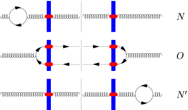
The resolution of this apparent paradox is in the fact that, while the particular set of diagrams in Fig. 3 does generate an additional leading logarithm of the center-of-mass energy $s$, such logarithms get canceled if we sum all the relevant diagrams, a possibility that has been encountered already in [71]. Consider diagrams in Figs. 4 and 8 which exhibit the same problem. For instance, diagram $C$ in Fig. 4 is UV divergent, while diagram $D$ in Fig. 4 is cut off by $s$ in the UV. Since the diagram in Fig. 4$D$ comes in with the overall minus sign compared to the diagram in Fig. 3$B$, as one of the quark-gluon vertices is moved to early time, we conclude that diagrams $C$ and $D$ in Fig. 4 give a contribution proportional to $-\ln(s/\mu)$. In the deep UV limit that we are studying the interactions of the quark bubble with the target are the same as the interactions of the gluon with the target: in the UV limit the quark and the anti-quark in the bubble would be very close to each other in transverse plane. Hence the remaining factors in the diagrams $C$ and $D$ in Fig. 4 are the same as those in the diagrams $A$, $B$ and $A^{\prime}$ in Fig. 3. Therefore the logarithms $\ln(s/\mu)$ cancel between diagrams 3 $A$, $B$, $A^{\prime}$ and diagrams 4 $C$, $D$. Similarly one can show that the logarithms $\ln(s/\mu)$ cancel between diagrams 8 $N$, $O$, $N^{\prime}$ and diagrams 4 $C^{\prime}$, $D^{\prime}$. In the end, all the extra logarithms of $s$ cancel, just as in the example of [71] for leading-order evolution.

In fact, the above observation applies to the leading-order small-$x$ evolution leading to the JIMWLK and BK equations [3, 4, 5, 6, 7, 8, 9, 10, 11, 12, 13, 14, 15]. There, in the forward amplitude, the diagrams with the gluon interacting with the target have a UV divergence, which should be regulated by the center-of-mass energy $s$. The diagrams with the virtual gluon have a divergence regulated simply by a cutoff. In the full evolution equation the divergences cancel between the real and virtual terms. To really see this, one has to gather all diagrams that become similar to the above in the UV to argue that logarithms of $s$ cancel as well. One might be tempted to argue that the diagrams like the one shown in Fig. 3 do not contribute to the forward amplitude. While this is true for generic momenta in the bulk of phase space, it is in fact not the case for the deep UV limit, where the transverse momenta of the quarks in the loop are large, making the light-cone lifetime of the quark bubble very short, shorter than the time interval between the multiple rescatterings in the target. Therefore such diagrams in this UV limit have to be included in the forward amplitude. However, due to the cancellation patterns observed above we see that all such deep-UV contributions cancel exactly (according to Eqs. (18), (21), (22), etc.), with the net effect that the sums of diagrams in Figs. 3, 4, etc., do not contribute to the forward amplitude, despite the fact that the individual diagrams would do so. In reality one has to be aware of this subtlety and remember that the diagrams under consideration do not contribute only because of an intricate cancellation.

We will now apply the machinery developed above to the calculation of running coupling corrections to the inclusive gluon production.

Now let us try to include running coupling corrections to the inclusive gluon production in the scattering of a small projectile on a large target. A diagram contributing to the gluon production cross section is shown in Fig. 9

in the notation introduced in the previous Section. The cross on the gluon line indicated that we tag on that gluon, keeping its momentum fixed.

To include the running coupling correction we have to again “dress” all gluon lines and vertices with quark bubbles. To begin with let us point out that $t$-channel gluon exchanges with the target get renormalized separately from the rest of the diagram: each $t$-channel gluon with transverse momentum $\bm{l}$ comes in with a factor of the bare coupling constant $\alpha_{\mu}$ and, after being dressed with fermion bubbles, it acquires the standard geometric series which can be absorbed in the denominator leading to the physical running coupling constant

$\displaystyle\alpha_{s}({\bm{l}}^{2})\,=\,\frac{\alpha_{\mu}}{1+\alpha_{\mu}\,\beta_{2}\,\ln\frac{{\bm{l}}^{2}}{\mu^{2}}}.$

(31)

The details of this calculation are shown in Appendix A, where we show how running coupling corrections enter into multiple gluon exchanges. There we consider dipole-nucleus scattering in the quasi-classical approximation. The results of the Appendix A, while directly applicable to DIS, can also be applied to gluon-target interactions shown in Fig. 9. Using the crossing symmetry one can show that the gluon-target interaction on both sides of the cut in Fig. 9 is equivalent to a gluon dipole–target interaction [38, 30] with the gluon dipole made out of the gluon lines on both sides of the cut. At large $N_{c}$ the gluon dipole is equivalent to two quark dipoles considered in Appendix A. We expect the structure of the running coupling corrections found in Appendix A for a quark dipole to be preserved for the gluon dipole beyond large $N_{c}$ limit.

It is interesting to note that the vertices where the $t$-channel gluon connects to the nucleons in the target come with a non-perturbative coupling, whose scale is determined by the typical momentum scale in each nucleon, i.e., by the scale of order of $\Lambda_{\text{QCD}}$. The vertices where the $t$-channel gluons couple to the projectile or to a gluon in the projectile’s wave function come with the coupling at the scale of the gluon’s transverse momentum and are, therefore, perturbative.

The important message for the discussion below is that the multiple rescatterings renormalize separately from the rest of the diagram. The only remaining factor of bare coupling comes from the gluon emission vertex. In Fig. 9 the gluon is emitted before the interaction on both sides of the cut. Since summation over emissions off of all quarks is implied in Fig. 9, the emission vertices are not shown explicitly. The two vertices give a factor of $\alpha_{\mu}$: our goal is to see how it transforms into a physical running coupling constant.

The gluon propagators at the light cone time before the interaction, $x_{+}<0$, can be dressed by quark bubbles both in the amplitude and in the complex conjugate amplitude, as shown in Fig. 10.

Both for Feynman diagrams and in LCPT such quark bubble chains would give a geometric series each. The two chains of bubbles would contribute a factor

$\displaystyle\frac{1}{\left[1+\alpha_{\mu}\,\beta_{2}\,\ln\frac{{\bm{r}}^{2}}{\mu^{2}}\right]\,\left[1+\alpha_{\mu}\,\beta_{2}\,\ln\frac{{\bm{r}^{\prime}}^{2}}{\mu^{2}}\right]}$

(32)

where $\bm{r}$ and $\bm{r}^{\prime}$ are the transverse momenta of the gluon before interaction with the target in the amplitude and in the complex conjugate amplitude, as shown in Fig. 10.

At the same time the vertices of the gluon interaction with the target could also have additive quark bubble (vertex) corrections. Adding the contributions of such bubbles gives a factor

$\displaystyle\left[1+\alpha_{\mu}\,\beta_{2}\,\ln\frac{{\bm{Q}}^{2}}{\mu^{2}}\right]\,\left[1+\alpha_{\mu}\,\beta_{2}\,\ln\frac{{\bm{Q}^{\prime}}^{2}}{\mu^{2}}\right]$

(33)

where $Q$ and $Q^{\prime}$ are some momentum scales characterizing the vertices (which, in the actual calculations are likely to become combinations of momenta of several gluon lines involved).

The combination of all bubble corrections in Fig. 10 and the bare coupling coming from the emission vertex is

$\displaystyle\alpha_{\mu}\,\frac{\left[1+\alpha_{\mu}\,\beta_{2}\,\ln\frac{{\bm{Q}}^{2}}{\mu^{2}}\right]\,\left[1+\alpha_{\mu}\,\beta_{2}\,\ln\frac{{\bm{Q}^{\prime}}^{2}}{\mu^{2}}\right]}{\left[1+\alpha_{\mu}\,\beta_{2}\,\ln\frac{{\bm{r}}^{2}}{\mu^{2}}\right]\,\left[1+\alpha_{\mu}\,\beta_{2}\,\ln\frac{{\bm{r}^{\prime}}^{2}}{\mu^{2}}\right]}\,=\,\alpha_{\mu}\,\frac{\alpha_{s}(r^{2})\,\alpha_{s}(r^{\prime 2})}{\alpha_{s}(Q^{2})\,\alpha_{s}(Q^{\prime 2})}.$

(34)

One can see that the bubble corrections of Fig. 10 still fail to turn the emission vertex coupling constant $\alpha_{\mu}$ into the physical running coupling constant. The only remaining bubble corrections which may complete $\alpha_{\mu}$ to a physical coupling constant are the bubble corrections placed on the outgoing gluon line in the final state.

The quark bubble chain corrections on the tagged gluon line are shown in Fig. 11. To sum them up we will use the result of Sect. 2 demonstrating that the sum of such corrections with the ones with the $q\bar{q}$ pair in the final state cancels. Therefore, the sum of all the diagrams with the gluon in the final state, like those shown in Fig. 11, is equal to the negative of the sum of all the diagrams with the $q\bar{q}$ pair in the final state, as illustrated in Fig. 12. The diagrams with the $q\bar{q}$ pair in the final state (on the right hand side of Fig. 12) have the advantage of not generating any singular energy denominators, like the ones discussed in Sect. 2.

While we can calculate the diagrams on the right hand side of Fig. 12 using LCPT, it is more straightforward to do so using the standard Feynman diagram technique. In Fig. 13 we show the amplitude with the $q\bar{q}$ pair in the final state and with the gluon line dressed by quark bubbles. Our discussion below will be restricted to the case when the gluon is emitted in the projectile before the interaction, as shown in Fig. 13. The conclusions we will obtain will be straightforward to generalize to the case of gluon emission after the interaction.

Let us consider massless quarks in the bubbles. In order to regulate collinear divergences, a study of which is our primary goal here, we will regulate the integral over the relative momentum of the $q\bar{q}$ pair in the final state with some infrared cutoff $\Lambda_{\text{coll}}$.

Completing the factor of $N_{f}$ coming from the fermion bubbles on the gluon line to the full beta-function by the replacement $N_{f}\rightarrow-6\pi\beta_{2}$ we obtain the following expression for the amplitude depicted in Fig. 13 (for similar calculations see [40, 17, 72])

$\displaystyle A\,=\,-\sum\limits_{\lambda=\pm 1}{\bm{M}}^{a}({\bm{q}},q_{+})\cdot{\bm{\epsilon}}^{\lambda}\,\frac{-i}{q^{2}+i\epsilon}\,\frac{4\,\pi\,\alpha_{\mu}}{1+\alpha_{\mu}\,\beta_{2}\,\left[\ln\left(-\frac{q^{2}+i\epsilon}{\mu_{\overline{\text{MS}}}^{2}}\right)-\frac{5}{3}\right]}\,t^{a}\,\frac{{\bm{\epsilon}}^{\lambda*}\cdot{\bm{k}}\,(1-2\alpha+\lambda\sigma)\,\delta_{\sigma,\sigma^{\prime}}}{\alpha\,(1-\alpha)\,q_{+}}.$

(35)

The notations used above are explained in Fig. 13: the outgoing quark and anti-quark have transverse momenta ${\bm{k}}_{1}$ and ${\bm{k}}_{2}$, while the gluon has 4-momentum $q_{\mu}$. The longitudinal fraction of the gluon’s momentum carried by the quark is

$\displaystyle\alpha\,\equiv\,\frac{k_{1+}}{q_{+}}\,=\,\frac{k_{1+}}{k_{1+}+k_{2+}}.$

(36)

In Eq. (35) we have defined

$\displaystyle{\bm{k}}\,\equiv\,(1-\alpha)\,{\bm{k}}_{1}-\alpha\,{\bm{k}}_{2}.$

(37)

The quark and anti-quark helicities are labeled $\sigma$ and $\sigma^{\prime}$ and the gluon polarization vector is $\epsilon_{\mu}^{\lambda}=(0,0,{\bm{\epsilon}}^{\lambda})$ with ${\bm{\epsilon}}^{\lambda}=(1+i\,\lambda)/\sqrt{2}$ and $\lambda=\pm 1$. In diagram shown in Fig. 13 only transverse gluon polarizations contribute. The gluon carries color $a$ and $t^{a}$ is the color matrix: summation over repeated indices is implied.

Remembering that outgoing quark and anti-quark are on mass shell and massless we write

$\displaystyle q^{2}=\frac{{\bm{k}}^{2}}{\alpha\,{\bar{\alpha}}}$

(38)

with ${\bar{\alpha}}=1-\alpha$.

The two-dimensional vector quantity ${\bm{M}}^{a}({\bm{q}},q_{+})$ denotes the part of the amplitude including the gluon emission and its interaction with the target. The fact that ${\bm{M}}^{a}({\bm{q}},q_{+})$ depends only on $\bm{q}$ and $q_{+}$, and is independent of $q^{2}$ (or, equivalently, $\bm{k}$), is most easily seen if this quantity is calculated in LCPT. There, all energy denominators in ${\bm{M}}^{a}({\bm{q}},q_{+})$ would not include any $\bm{k}$-dependence since ${\bm{M}}^{a}({\bm{q}},q_{+})$ includes only the initial state dynamics and $\bm{k}$ is the final state momentum. The factor of the coupling constant $g$ due to gluon emission by the projectile is not included in ${\bm{M}}^{a}({\bm{q}},q_{+})$ and is shown explicitly in Eq. (35) as one of the two factors of $g$ giving $\alpha_{\mu}$ in the numerator.

As $q^{2}={\bm{k}}^{2}/\alpha\,{\bar{\alpha}}\geq 0$, and, since later on we will regulate the collinear divergence at $\bm{k}=0$ with a cutoff $\Lambda_{\text{coll}}$, we drop the $i\epsilon$ regulators in Eq. (35) obtaining

$\displaystyle A\,=\,\sum\limits_{\lambda=\pm 1}{\bm{M}}^{a}({\bm{q}},q_{+})\cdot{\bm{\epsilon}}^{\lambda}\,\frac{i}{q^{2}}\,\frac{4\,\pi\,\alpha_{\mu}}{1+\alpha_{\mu}\,\beta_{2}\,\left[\ln\left(-\frac{q^{2}}{\mu_{\overline{\text{MS}}}^{2}}\right)-\frac{5}{3}\right]}\,t^{a}\,\frac{{\bm{\epsilon}}^{\lambda*}\cdot{\bm{k}}\,(1-2\alpha+\lambda\sigma)\,\delta_{\sigma,\sigma^{\prime}}}{\alpha\,{\bar{\alpha}}\,q_{+}}.$

(39)

As the gluon is space-like, $q^{2}>0$, the amplitude in Eq. (39) has an imaginary part corresponding to the $q\bar{q}$ pair in any one of the fermion bubbles dressing up the gluon line going on mass shell. However, this imaginary part does not contain any ultraviolet divergence and hence does not contribute to running coupling corrections. We will neglect it along with the $5/3$ in the denominator of Eq. (39) and rewrite the amplitude as

$\displaystyle A\,$

$\displaystyle=\,4\,\pi\,i\,\sum\limits_{\lambda=\pm 1}{\bm{M}}^{a}({\bm{q}},q_{+})\cdot{\bm{\epsilon}}^{\lambda}\,\frac{\alpha_{s}(q^{2})}{q^{2}}\,t^{a}\,\frac{{\bm{\epsilon}}^{\lambda*}\cdot{\bm{k}}\,(1-2\alpha+\lambda\sigma)\,\delta_{\sigma,\sigma^{\prime}}}{\alpha\,{\bar{\alpha}}\,q_{+}}.$

(40)

Multiplying the amplitude (40) by its complex conjugate and summing over colors, quark helicities $\sigma$, $\sigma^{\prime}$ and $N_{f}$ quark flavors (assuming all flavors are massless) yields the amplitude squared

	$\displaystyle|A|^{2}\,=\,(4\,\pi)^{2}\sum\limits_{\lambda,\lambda^{\prime}=\pm 1}$	$\displaystyle{\bm{M}}^{a}({\bm{q}},q_{+})\cdot{\bm{\epsilon}}^{\lambda}\ {\bm{M}}^{a*}({\bm{q}},q_{+})\cdot{\bm{\epsilon}}^{\lambda^{\prime}*}\,\left(\frac{\alpha_{s}(q^{2})}{q^{2}}\right)^{2}\,\frac{N_{f}}{\alpha^{2}\,{\bar{\alpha}}^{2}\,q_{+}^{2}}$
		$\displaystyle\times\,{\bm{\epsilon}}^{\lambda*}\cdot{\bm{k}}\ {\bm{\epsilon}}^{\lambda^{\prime}}\cdot{\bm{k}}\,[(1-2\alpha)^{2}+\lambda\,\lambda^{\prime}].$		(41)

To calculate the contribution to the gluon production cross section of diagrams with the outgoing gluon line dressed with quark bubbles to all orders (but excluding the contribution of the bare outgoing gluon line) we use the identity pictured in Fig. 12: we flip the sign of the amplitude squared in Eq. (3) and integrate over $\bm{k}$ and $\alpha$. The contribution to the total cross section of the square of the diagram in Fig. 13 comes with the integration measure

$\displaystyle\frac{d^{2}k_{1}\,dk_{1+}\,d^{2}k_{2}\,dk_{2+}}{2(2\pi)^{3}\,2(2\pi)^{3}}\,=\,\frac{d^{2}q\,d^{2}k\,dq_{+}\,d\alpha\,q_{+}}{2(2\pi)^{3}\,2(2\pi)^{3}}.$

(42)

Defining the gluon’s rapidity $y$ by

$\displaystyle y\,=\,\frac{1}{2}\,\ln\frac{q_{+}}{q_{-}}\,=\,\ln\frac{q_{+}\,\sqrt{2}}{q_{T}}$

(43)

with $q_{T}=|{\bm{q}}|$ we write the contribution of the diagram on the left hand side of Fig. 12 to the multiplicity of produced gluons as

$\displaystyle\frac{dN^{G}_{\text{bubbles}}}{d^{2}q\,dy}\,=\,-\int\frac{d^{2}k}{4(2\pi)^{6}}\,\int\limits_{0}^{1}d\alpha\,q_{+}^{2}\,|A|^{2}.$

(44)

The integral over $\bm{k}$ in Eq. (44) comes with an infrared regulator $\Lambda_{\text{coll}}$: the domain of integration is restricted to $k_{T}>\Lambda_{\text{coll}}$. On the other hand, when arriving at Eq. (35) one effectively integrates over momenta in the (uncut) quark bubbles up to the ultraviolet (UV) cutoff $\mu_{\overline{\text{MS}}}$. Therefore, to keep the integration over $k_{T}$ in the cut bubble in Fig. 13 in agreement with the similar integrals in other (uncut) quark bubbles and thus to keep Fig. 12 valid by restricting all quark bubbles to the same phase space, we will introduce this UV cutoff and put another restriction on the range of integration: $k_{T}<\mu_{\overline{\text{MS}}}$ . It is important to stress once more that Eq. (44) does not contain the contribution of the bare outgoing gluon line.

Indeed the equality in Fig. 12 is true without any infrared cutoffs on $k_{T}$ integration. In other words, the integral over $\bm{k}$ of the cut bubble on the right of Fig. 12 is, in general, not restricted to $k_{T}>\Lambda_{\text{coll}}$. One can think of the right hand side of Fig. 12 as consisting of the sum of the $k_{T}>\Lambda_{\text{coll}}$ and $k_{T}<\Lambda_{\text{coll}}$ contributions (with an overall minus sign). In Eq. (44) we only keep the $k_{T}>\Lambda_{\text{coll}}$ contribution. Due to Fig. 12 it is equal to the sum of gluon production and the $q\bar{q}$ production with $k_{T}<\Lambda_{\text{coll}}$. Now the meaning of the multiplicity in Eq. (44) becomes clear: it is the net number of produced gluons and collinear $q\bar{q}$ pairs with $k_{T}<\Lambda_{\text{coll}}$. For simplicity we will refer to the obtained multiplicity distribution as “gluon” multiplicity below, but we will always keep in mind that collinear $q\bar{q}$ pairs with $k_{T}<\Lambda_{\text{coll}}$ are included in it as well.

Replacing $N_{f}\rightarrow-6\pi\beta_{2}$ in Eq. (3), plugging the result into Eq. (44) we integrate over the angles of $\bm{k}$ and using Eq. (38) for $q^{2}$ get

$\displaystyle\frac{dN^{G}_{\text{bubbles}}}{d^{2}q\,dy}\,=\,\frac{6\,\pi^{2}\,\beta_{2}}{(2\,\pi)^{4}}\ |{\bm{M}}^{a}({\bm{q}},q_{+})|^{2}\,\int\limits_{0}^{1}d\alpha\,\int\limits_{\Lambda_{\text{coll}}^{2}}^{\mu_{\overline{\text{MS}}}^{2}}dk_{T}^{2}\,\left(\frac{\alpha_{s}(k_{T}^{2}/\alpha\,{\bar{\alpha}})}{k_{T}^{2}}\right)^{2}\,\frac{1}{2}\ k_{T}^{2}\,[(1-2\alpha)^{2}+1].$

(45)

It is interesting to observe that the argument of the running coupling in Eq. (45) is similar to that of the coupling in the Dokshitzer-Gribov-Lipatov-Altarelli-Parisi (DGLAP) evolution equation [73, 74, 75] as was calculated in [76].

Using

$\displaystyle\alpha_{s}(Q^{2})\,=\,\frac{1}{\beta_{2}\,\ln\frac{Q^{2}}{\Lambda_{\text{QCD}}^{2}}}$

(46)

we integrate Eq. (45) over $k_{T}^{2}$. The result of the integration yields

$\displaystyle\frac{dN^{G}_{\text{bubbles}}}{d^{2}q\,dy}\,=\,\frac{3\,\pi^{2}}{(2\,\pi)^{4}}\,|{\bm{M}}^{a}({\bm{q}},q_{+})|^{2}\,\int\limits_{0}^{1}d\alpha\,[(1-2\alpha)^{2}+1]\ \left[\alpha_{s}\!\left(\frac{\Lambda_{\text{coll}}^{2}}{\alpha\,{\bar{\alpha}}}\right)-\alpha_{s}\!\left(\frac{\mu_{\overline{\text{MS}}}^{2}}{\alpha\,{\bar{\alpha}}}\right)\right].$

(47)

The part of the $\alpha$-integral in Eq. (47) involving the factor of $\alpha\,{\bar{\alpha}}$ in the argument of the coupling constants contributes only to fixing the constant under the logarithm. In the spirit of BLM approach [51] we can expand the coupling constants in Eq. (47) into geometric series, integrate each (of the first few) terms over $\alpha$, and then resum back the series. $\alpha\,{\bar{\alpha}}$ terms in the argument of the couplings will only contribute constants to the terms in the series: since we are not keeping track of constant terms we will simply neglect them. Integrating the prefactor in Eq. (47) over $\alpha$ and neglecting other irrelevant constants in the argument of the second coupling we write for the contribution to the produced gluon multiplicity

$\displaystyle\frac{dN^{G}_{\text{bubbles}}}{d^{2}q\,dy}\,=\,\frac{1}{(2\,\pi)^{2}}\,|{\bm{M}}^{a}({\bm{q}},q_{+})|^{2}\ \left[\alpha_{s}\!\left(\Lambda_{\text{coll}}^{2}\right)-\alpha_{\mu}\right].$

(48)

Finally, adding the contribution of the bare outgoing gluon line

$\displaystyle\frac{dN^{G}_{\text{bare}}}{d^{2}q\,dy}\,=\,\frac{1}{2\,(2\,\pi)^{3}}\,|{\bm{M}}^{a}({\bm{q}},q_{+})|^{2}\ g^{2}_{\mu}\,=\,\frac{1}{(2\,\pi)^{2}}\,|{\bm{M}}^{a}({\bm{q}},q_{+})|^{2}\ \alpha_{\mu}$

(49)

(with $g_{\mu}$ the bare coupling constant $g$) to the contribution of Eq. (48) we obtain the following expression for the produced gluon (and collinear $q\bar{q}$ pairs) multiplicity with the running coupling corrections included:

$\displaystyle\frac{dN^{G}}{d^{2}q\,dy}\,=\,\frac{1}{(2\,\pi)^{2}}\,|{\bm{M}}^{a}({\bm{q}},q_{+})|^{2}\ \alpha_{s}\!\left(\Lambda_{\text{coll}}^{2}\right).$

(50)

(Note that Eq. (50) can be obtained directly from Eq. (45) by setting the upper limit of the $\bm{k}$-integration to infinity. As follows from our derivation above, doing this would modify Eq. (45) to include the contribution of the bare gluon line. Similar observation has been made before for other production processes in [77, 56].)

From Eq. (50) we can draw the following conclusions:

• •

  First of all, we have shown that the bare coupling constant $\alpha_{\mu}$ stemming from the vertices of gluon emission by the projectile in the amplitude and in the complex conjugate amplitude gets renormalized into a physical coupling constant. We have thus outlined the procedure of how running coupling corrections should be included into the gluon production cross section.

• •

  Unfortunately the scale with which the coupling runs in Eq. (50) is some arbitrary infrared cutoff $\Lambda_{\text{coll}}$ which we introduced to regulate collinear divergences. This makes the gluon production cross section (or, equivalently, gluon multiplicity) either perturbative or non-perturbative depending on the choice of the cutoff $\Lambda_{\text{coll}}$ corresponding to the resolution scale for gluons and $q\bar{q}$ pairs. Strictly speaking this means that the gluon multiplicity is not infrared-safe, in accordance with conventional wisdom.

Indeed the dependence of the gluon multiplicity on $\Lambda_{\text{coll}}$ is already weakened by that fact that it is absorbed in the argument of a running coupling constant. The $\Lambda_{\text{coll}}$-dependence could be further reduced by performing a Sudakov-like resummation [78] of gluon splittings. If the goal of a calculation is to find the cross section for production of hadrons, it may be possible to absorb the result of such resummation into a fragmentation function. However, performing a Sudakov resummation on top of the calculation of the running coupling corrections appears to be rather involved and is beyond the scope of this work.

The resolution scale $\Lambda_{\text{coll}}$ generates an IR cutoff on $k_{T}$ of the produced quarks in Eq. (45). Due to Eq. (38) this translates into a cutoff on gluon virtuality $q^{2}$, which is equal to the invariant mass of the $q\bar{q}$ pair. Neglecting $\alpha\,{\bar{\alpha}}$ we could say that $q\bar{q}$ pairs with the invariant mass $q^{2}\lesssim\Lambda_{\text{coll}}^{2}$ are included into our definition of gluon multiplicity distribution.

However, one should be aware that our calculation is reliable only as long as $\Lambda_{\text{coll}}^{2}$ remains in the perturbative domain and that, if one is forced to take $\Lambda_{\text{coll}}^{2}$ closer to $\Lambda_{\text{QCD}}^{2}$ on phenomenological grounds, the only consistent way to take into account the non-perturbative contributions – and the nontrivial true dependence on $\Lambda_{\text{coll}}^{2}$ in the non-perturbative region – is to introduce a factorization procedure that subsumes these contributions in a fragmentation function whose $\Lambda_{\text{coll}}^{2}$ dependence can only be inferred with non-perturbative means or by comparison with experiment. This introduces a factorization scale $\mu^{2}$ between perturbative contributions above it and non-perturbative ones below. The former are reliably reproduced by our calculation if we substitute the perturbative factorization scale $\mu^{2}$ in place of $\Lambda_{\text{coll}}^{2}$ in the above.³³ 3 In such a setting, one has to keep in mind that the factorization scale, while infrared from the perspective of the perturbative contribution, is in the UV from the perspective of the modes entering the operator defining the fragmentation functions [62, 63] and may be thought of as its renormalization scale $\mu$, which, in general, is different from full UV renormalization scale $\mu_{\overline{\text{MS}}}$ for the complete graph. Fragmentation functions depend both on the factorization scale $\mu$ and on the collinear IR cutoff $\Lambda_{\text{coll}}$. The perturbative part of the cross section depends on the renormalization scale $\mu_{\overline{\text{MS}}}$ and on the factorization scale $\mu$. In the full hadron production cross section the $\mu$-dependence cancels so that it only depends on $\mu_{\overline{\text{MS}}}$ and $\Lambda_{\text{coll}}$. For heavy quark–anti-quark bound state production the factorization scale is chosen to be equal to the lowest possible value of the invariant mass of the $q\bar{q}$ pair [79], which is not too different from the cutoff on the invariant mass obtained above. Still, the introduction of fragmentation functions is necessary for consistency even in such a case where the non-perturbative contributions become (almost) trivial.

In practical phenomenological calculations of hadron production one often chooses the factorization scale $\mu\sim p_{T}$ with $p_{T}$ the transverse momentum of the produced hadron. In this case, Eq. (50) should be convoluted with the fragmentation functions and $\Lambda_{\text{coll}}$ in it should be replaced by the factorization scale $\mu$. If one puts $\mu\sim p_{T}$ one would then get $\alpha_{s}(p_{T}^{2})$ in Eq. (50). While in an all-order calculation the hadron production cross section should not depend on the choice of the factorization scale $\mu$, in practical applications putting $\mu\sim p_{T}$ in our result would lead to some additional $p_{T}$-dependence.

Our goal now is to verify that while gluon (and quark) multiplicity is not infrared-finite, the energy density of the medium produced in the collision is infrared-finite. The energy density $\epsilon$ is given by Eq. (5). With the gluon multiplicity being infinite, there are at least two ways the net energy density could stay finite:

• (i)

  it may be that the sum of gluon and quark multiplicities (net parton multiplicity) is finite, or

• (ii)

  it may be that the divergence in the sum of gluon and quark multiplicities vanishes after the integration over the transverse momentum in Eq. (5).

To calculate the energy density using Eq. (5) we need the expressions for gluon and quark multiplicities. For the gluon multiplicity we have Eq. (50). To calculate the contribution of the diagram in Fig. 13 to the quark production cross section, we simply have to take the expression in Eq. (45), flip its sign back (to undo the sign flip shown on the right hand side of Fig. 12) and instead of integrating over $\bm{k}$ and $\alpha$ we would integrate over momenta of the anti-quark keeping the transverse momentum and rapidity of the quark fixed. We get

$\displaystyle\frac{dN^{q}}{d^{2}p\,dy}\,=\,-\frac{1}{(2\,\pi)^{4}}\int d^{2}k_{1}\,d^{2}k_{2}\,\frac{dk_{1+}\,dk_{2+}}{q_{+}^{2}}\,\delta({\bm{p}}-{\bm{k}}_{1})\,\delta\!\left(y-\ln\frac{k_{1+}\,\sqrt{2}}{k_{1T}}\right)\,|{\bm{M}}^{a}({\bm{q}},q_{+})|^{2}\,f({\bm{k}};\alpha,{\bar{\alpha}})$

(51)

were we have defined

$\displaystyle f({\bm{k}};\alpha,{\bar{\alpha}})\,=\,6\,\pi\,\beta_{2}\,\left(\frac{\alpha_{s}(k_{T}^{2}/\alpha\,{\bar{\alpha}})}{k_{T}^{2}}\right)^{2}\,\frac{1}{2}\ k_{T}^{2}\,[(\alpha-{\bar{\alpha}})^{2}+1].$

(52)

The produced quark’s rapidity is given by $y=\ln(p_{+}\,\sqrt{2}/p_{T})$, same as Eq. (43) for the gluon rapidity. Note that $f({\bm{k}};\alpha,{\bar{\alpha}})$ is symmetric under the interchange $\alpha\leftrightarrow{\bar{\alpha}}$: $f({\bm{k}};\alpha,{\bar{\alpha}})=f({\bm{k}};{\bar{\alpha}},\alpha)$.

Strictly speaking to calculate quark production we would have to replace $-6\,\pi\,\beta_{2}$ in Eq. (52) (and, consequently, in Eq. (51)) back with $N_{f}$. However we will leave $\beta_{2}$ intact in Eq. (52). By doing so we will indeed include the cut gluon bubble into Eq. (51) making the expression in Eq. (51) include both quark multiplicity and the multiplicity of gluons coming from a cut gluon bubble correction. Indeed if we want to see cancellation or disappearance of collinear singularities, we need to sum both (anti-)quark and gluon contributions. Hence, in our notation, the ”quark multiplicity” would include both quark and gluon multiplicity coming from the cut bubbles.

Eliminating the delta-functions in Eq. (51) we write

$\displaystyle\frac{dN^{q}}{d^{2}p\,dy}\,=\,-\frac{1}{(2\,\pi)^{4}}\int d^{2}k_{2}\,\int\limits_{0}^{1}\,d\alpha\,\bigg|{\bm{M}}^{a}\left({\bm{p}}+{\bm{k}}_{2},\frac{p_{T}\,e^{y}}{\alpha\,\sqrt{2}}\right)\bigg|^{2}\,f({\bar{\alpha}}\,{\bm{p}}-\alpha\,{\bm{k}}_{2};\alpha,{\bar{\alpha}})$

(53)

were, in accordance with Eq. (36), we have used

$\displaystyle\alpha\,=\,\frac{p_{+}}{p_{+}+k_{2+}}.$

(54)

The anti-quark multiplicity is obtained from the multiplicity of the quarks in (53) by replacing $\alpha\leftrightarrow{\bar{\alpha}}$ and ${\bm{k}}_{2}\rightarrow{\bm{k}}_{1}$. We get

$\displaystyle\frac{dN^{\bar{q}}}{d^{2}p\,dy}\,=\,-\frac{1}{(2\,\pi)^{4}}\int d^{2}k_{1}\,\int\limits_{0}^{1}\,d\alpha\,\bigg|{\bm{M}}^{a}\left({\bm{p}}+{\bm{k}}_{1},\frac{p_{T}\,e^{y}}{{\bar{\alpha}}\,\sqrt{2}}\right)\bigg|^{2}\,f({\alpha}\,{\bm{p}}-{\bar{\alpha}}\,{\bm{k}}_{1};\alpha,{\bar{\alpha}}).$

(55)

With the help of Eqs. (45) and (52) we rewrite Eq. (50) as

$\displaystyle\frac{dN^{G}}{d^{2}p\,dy}\,=\,\frac{1}{(2\,\pi)^{4}}\int d^{2}k\,\int\limits_{0}^{1}\,d\alpha\,\bigg|{\bm{M}}^{a}\left({\bm{p}},\frac{p_{T}\,e^{y}}{\sqrt{2}}\right)\bigg|^{2}\,f({\bm{k}};\alpha,{\bar{\alpha}})$

(56)

where now the integral over $k_{T}$ is not bounded by the cutoff $\mu_{\overline{\text{MS}}}$ from above. As was discussed in the previous section this insures that the contribution of the bare outgoing gluon line is included in Eq. (56) as well.

References

- [1] E. A. Kuraev, L. N. Lipatov, and V. S. Fadin, The Pomeranchuk singularity in non-Abelian gauge theories, Sov. Phys. JETP 45 (1977) 199–204.
- [2] Y. Y. Balitsky and L. N. Lipatov Sov. J. Nucl. Phys. 28 (1978) 822.
- [3] I. Balitsky, Operator expansion for high-energy scattering, Nucl. Phys. B463 (1996) 99–160, [hep-ph/9509348].
- [4] I. Balitsky, Operator expansion for diffractive high-energy scattering, hep-ph/9706411.
- [5] I. Balitsky, Factorization and high-energy effective action, Phys. Rev. D60 (1999) 014020, [hep-ph/9812311].
- [6] Y. V. Kovchegov, Small-x structure function of a nucleus including multiple pomeron exchanges, Phys. Rev. D60 (1999) 034008, [hep-ph/9901281].
- [7] Y. V. Kovchegov, Unitarization of the BFKL pomeron on a nucleus, Phys. Rev. D61 (2000) 074018, [hep-ph/9905214].
- [8] J. Jalilian-Marian, A. Kovner, A. Leonidov, and H. Weigert, The BFKL equation from the Wilson renormalization group, Nucl. Phys. B504 (1997) 415–431, [hep-ph/9701284].
- [9] J. Jalilian-Marian, A. Kovner, A. Leonidov, and H. Weigert, The Wilson renormalization group for low x physics: Towards the high density regime, Phys. Rev. D59 (1998) 014014, [hep-ph/9706377].
- [10] J. Jalilian-Marian, A. Kovner, and H. Weigert, The Wilson renormalization group for low x physics: Gluon evolution at finite parton density, Phys. Rev. D59 (1998) 014015, [hep-ph/9709432].
- [11] J. Jalilian-Marian, A. Kovner, A. Leonidov, and H. Weigert, Unitarization of gluon distribution in the doubly logarithmic regime at high density, Phys. Rev. D59 (1999) 034007, [hep-ph/9807462].
- [12] A. Kovner, J. G. Milhano, and H. Weigert, Relating different approaches to nonlinear QCD evolution at finite gluon density, Phys. Rev. D62 (2000) 114005, [hep-ph/0004014].
- [13] H. Weigert, Unitarity at small Bjorken x, Nucl. Phys. A703 (2002) 823–860, [hep-ph/0004044].
- [14] E. Iancu, A. Leonidov, and L. D. McLerran, Nonlinear gluon evolution in the color glass condensate. I, Nucl. Phys. A692 (2001) 583–645, [hep-ph/0011241].
- [15] E. Ferreiro, E. Iancu, A. Leonidov, and L. McLerran, Nonlinear gluon evolution in the color glass condensate. II, Nucl. Phys. A703 (2002) 489–538, [hep-ph/0109115].
- [16] I. I. Balitsky, Quark Contribution to the Small- Evolution of Color Dipole, Phys. Rev. D 75 (2007) 014001, [hep-ph/0609105].
- [17] Y. Kovchegov and H. Weigert, Triumvirate of Running Couplings in Small- Evolution, Nucl. Phys. A 784 (2007) 188–226, [hep-ph/0609090].
- [18] Y. V. Kovchegov and H. Weigert, Quark loop contribution to BFKL evolution: Running coupling and leading-N(f) NLO intercept, accepted for publication at Nucl. Phys. A (2006) [hep-ph/0612071].
- [19] J. L. Albacete and Y. V. Kovchegov, Solving high energy evolution equation including running coupling corrections, Phys. Rev. D75 (2007) 125021, [arXiv:0704.0612 [hep-ph]].
- [20] L. V. Gribov, E. M. Levin, and M. G. Ryskin, Semihard Processes in QCD, Phys. Rept. 100 (1983) 1–150.
- [21] A. H. Mueller and J.-w. Qiu, Gluon recombination and shadowing at small values of x, Nucl. Phys. B268 (1986) 427.
- [22] L. D. McLerran and R. Venugopalan, Green’s functions in the color field of a large nucleus, Phys. Rev. D50 (1994) 2225–2233, [hep-ph/9402335].
- [23] L. D. McLerran and R. Venugopalan, Gluon distribution functions for very large nuclei at small transverse momentum, Phys. Rev. D49 (1994) 3352–3355, [hep-ph/9311205].
- [24] L. D. McLerran and R. Venugopalan, Computing quark and gluon distribution functions for very large nuclei, Phys. Rev. D49 (1994) 2233–2241, [hep-ph/9309289].
- [25] Y. V. Kovchegov, Non-abelian Weizsaecker-Williams field and a two- dimensional effective color charge density for a very large nucleus, Phys. Rev. D54 (1996) 5463–5469, [hep-ph/9605446].
- [26] Y. V. Kovchegov, Quantum structure of the non-abelian Weizsaecker-Williams field for a very large nucleus, Phys. Rev. D55 (1997) 5445–5455, [hep-ph/9701229].
- [27] J. Jalilian-Marian, A. Kovner, L. D. McLerran, and H. Weigert, The intrinsic glue distribution at very small x, Phys. Rev. D55 (1997) 5414–5428, [hep-ph/9606337].
- [28] E. Iancu and R. Venugopalan, The color glass condensate and high energy scattering in QCD, hep-ph/0303204.
- [29] H. Weigert, Evolution at small : The Color Glass Condensate, Prog. Part. Nucl. Phys. 55 (2005) 461–565, [hep-ph/0501087].
- [30] J. Jalilian-Marian and Y. V. Kovchegov, Saturation physics and deuteron gold collisions at RHIC, Prog. Part. Nucl. Phys. 56 (2006) 104–231, [hep-ph/0505052].
- [31] A. Kovner, L. D. McLerran, and H. Weigert, Gluon production from nonAbelian Weizsacker-Williams fields in nucleus-nucleus collisions, Phys. Rev. D52 (1995) 6231–6237, [hep-ph/9502289].
- [32] A. Kovner, L. D. McLerran, and H. Weigert, Gluon production at high transverse momentum in the mclerran-venugopalan model of nuclear structure functions, Phys. Rev. D52 (1995) 3809–3814, [hep-ph/9505320].
- [33] M. Gyulassy and L. D. McLerran, Yang-mills radiation in ultrarelativistic nuclear collisions, Phys. Rev. C56 (1997) 2219–2228, [nucl-th/9704034].
- [34] Y. V. Kovchegov and D. H. Rischke, Classical gluon radiation in ultrarelativistic nucleus nucleus collisions, Phys. Rev. C56 (1997) 1084–1094, [hep-ph/9704201].
- [35] Y. V. Kovchegov and A. H. Mueller, Gluon production in current nucleus and nucleon nucleus collisions in a quasi-classical approximation, Nucl. Phys. B529 (1998) 451–479, [hep-ph/9802440].
- [36] B. Z. Kopeliovich, A. V. Tarasov, and A. Schafer, Bremsstrahlung of a quark propagating through a nucleus, Phys. Rev. C59 (1999) 1609–1619, [hep-ph/9808378].
- [37] A. Dumitru and L. D. McLerran, How protons shatter colored glass, Nucl. Phys. A700 (2002) 492–508, [hep-ph/0105268].
- [38] Y. V. Kovchegov and K. Tuchin, Inclusive gluon production in dis at high parton density, Phys. Rev. D65 (2002) 074026, [hep-ph/0111362].
- [39] F. Gelis and J. Jalilian-Marian, From dis to proton nucleus collisions in the color glass condensate model, Phys. Rev. D67 (2003) 074019, [hep-ph/0211363].
- [40] Y. V. Kovchegov and K. Tuchin, Production of q anti-q pairs in proton nucleus collisions at high energies, hep-ph/0603055.
- [41] Y. V. Kovchegov, Inclusive gluon production in high energy onium onium scattering, Phys. Rev. D72 (2005) 094009, [hep-ph/0508276].
- [42] A. Dumitru and J. Jalilian-Marian, Scattering of gluons from the color glass condensate, Phys. Lett. B547 (2002) 15–20, [hep-ph/0111357].
- [43] A. Dumitru and J. Jalilian-Marian, Forward quark jets from protons shattering the colored glass, Phys. Rev. Lett. 89 (2002) 022301, [hep-ph/0204028].
- [44] A. Kovner and U. A. Wiedemann, Eikonal evolution and gluon radiation, Phys. Rev. D64 (2001) 114002, [hep-ph/0106240].
- [45] J. P. Blaizot, F. Gelis, and R. Venugopalan, High energy p A collisions in the color glass condensate approach. I: Gluon production and the Cronin effect, Nucl. Phys. A743 (2004) 13–56, [hep-ph/0402256].
- [46] C. Marquet, A QCD dipole formalism for forward-gluon production, Nucl. Phys. B705 (2005) 319–338, [hep-ph/0409023].
- [47] F. Gelis and Y. Mehtar-Tani, Gluon propagation inside a high-energy nucleus, Phys. Rev. D73 (2006) 034019, [hep-ph/0512079].
- [48] L. V. Gribov, E. M. Levin, and M. G. Ryskin, Singlet structure function at small x: Unitarization of gluon ladders, Nucl. Phys. B188 (1981) 555–576.
- [49] S. Catani, M. Ciafaloni, and F. Hautmann, High-energy factorization and small x heavy flavor production, Nucl. Phys. B366 (1991) 135–188.
- [50] D. Kharzeev, Y. V. Kovchegov, and K. Tuchin, Cronin effect and high-p(t) suppression in p a collisions, Phys. Rev. D68 (2003) 094013, [hep-ph/0307037].
- [51] S. J. Brodsky, G. P. Lepage, and P. B. Mackenzie, On the elimination of scale ambiguities in perturbative quantum chromodynamics, Phys. Rev. D28 (1983) 228.
- [52] A. H. Mueller, On the structure of infrared renormalons in physical processes at high-energies, Nucl. Phys. B250 (1985) 327.
- [53] G. Parisi, Singularities of the borel transform in renormalizable theories, Phys. Lett. B76 (1978) 65–66.
- [54] F. David, On the ambiguity of composite operators, I.R. renormalons and the status of the operator product expansion, Nucl. Phys. B234 (1984) 237–251.
- [55] V. I. Zakharov, QCD perturbative expansions in large orders, Nucl. Phys. B385 (1992) 452–480.
- [56] M. Beneke, Renormalons, Phys. Rept. 317 (1999) 1–142, [hep-ph/9807443].
- [57] M. Beneke and V. M. Braun, Renormalons and power corrections, hep-ph/0010208.
- [58] M. Beneke and V. M. Braun, Naive nonAbelianization and resummation of fermion bubble chains, Phys. Lett. B348 (1995) 513–520, [hep-ph/9411229].
- [59] B. Lautrup, On high order estimates in qed, Phys. Lett. B69 (1977) 109–111.
- [60] G. ’t Hooft, Can we make sense out of ’quantum chromodynamics’?, . Lectures given at Int. School of Subnuclear Physics, Erice, Sicily, Jul 23 - Aug 10, 1977.
- [61] I. Balitsky and G. A. Chirilli, Next-to-leading order evolution of color dipoles, Phys. Rev. D77 (2008) 014019, [0710.4330].
- [62] E. L. Berger, X.-f. Guo, and J.-w. Qiu, Isolated prompt photon production in hadronic final states of annihilation, Phys. Rev. D54 (1996) 5470–5495, [hep-ph/9605324].
- [63] E. L. Berger, X.-F. Guo, and J.-W. Qiu, Inclusive prompt photon production in hadronic final states of e+ e- annihilation, Phys. Rev. D53 (1996) 1124–1141, [hep-ph/9507428].
- [64] Y. V. Kovchegov, Can thermalization in heavy ion collisions be described by QCD diagrams?, Nucl. Phys. A762 (2005) 298–325, [hep-ph/0503038].
- [65] A. H. Mueller, Small x Behavior and Parton Saturation: A QCD Model, Nucl. Phys. B335 (1990) 115.
- [66] E. Gardi, J. Kuokkanen, K. Rummukainen, and H. Weigert, Running coupling and power corrections in nonlinear evolution at the high-energy limit, Nucl. Phys. A784 (2007) 282–340, [hep-ph/0609087].
- [67] J. Jalilian-Marian and Y. V. Kovchegov, Inclusive two-gluon and valence quark-gluon production in DIS and p A, Phys. Rev. D70 (2004) 114017, [hep-ph/0405266].
- [68] Z. Chen and A. H. Mueller, The dipole picture of high-energy scattering, the BFKL equation and many gluon compound states, Nucl. Phys. B451 (1995) 579–604.
- [69] G. P. Lepage and S. J. Brodsky, Exclusive processes in perturbative quantum chromodynamics, Phys. Rev. D22 (1980) 2157.
- [70] S. J. Brodsky, H.-C. Pauli, and S. S. Pinsky, Quantum chromodynamics and other field theories on the light cone, Phys. Rept. 301 (1998) 299–486, [hep-ph/9705477].
- [71] A. Babansky and I. Balitsky, Scattering of color dipoles: From low to high energies, Phys. Rev. D67 (2003) 054026, [hep-ph/0212075].
- [72] Y. V. Kovchegov and L. D. McLerran, Diffractive structure function in a quasi-classical approximation, Phys. Rev. D60 (1999) 054025, [hep-ph/9903246].
- [73] Y. L. Dokshitzer, Calculation of the structure functions for deep inelastic scattering and e+ e- annihilation by perturbation theory in quantum chromodynamics. (in russian), Sov. Phys. JETP 46 (1977) 641–653.
- [74] V. N. Gribov and L. N. Lipatov, Deep inelastic e p scattering in perturbation theory, Sov. J. Nucl. Phys. 15 (1972) 438–450.
- [75] G. Altarelli and G. Parisi, Asymptotic freedom in parton language, Nucl. Phys. B126 (1977) 298.
- [76] Y. L. Dokshitzer and D. V. Shirkov, On exact account of heavy quark thresholds in hard processes, Z. Phys. C67 (1995) 449–458.
- [77] M. Beneke and V. M. Braun, Power corrections and renormalons in Drell-Yan production, Nucl. Phys. B454 (1995) 253–290, [hep-ph/9506452].
- [78] V. V. Sudakov, Vertex parts at very high-energies in quantum electrodynamics, Sov. Phys. JETP 3 (1956) 65–71.
- [79] E. Braaten and T. C. Yuan, Gluon fragmentation into heavy quarkonium, Phys. Rev. Lett. 71 (1993) 1673–1676, [hep-ph/9303205].
- [80] J. Kwiecinski, A. D. Martin, P. J. Sutton, and K. J. Golec-Biernat, QCD predictions for the transverse energy flow in deep inelastic scattering in the HERA small x regime, Phys. Rev. D50 (1994) 217–225, [hep-ph/9403292].
- [81] A. L. Ayala, M. B. Gay Ducati, and E. M. Levin, Qcd evolution of the gluon density in a nucleus, Nucl. Phys. B493 (1997) 305–353, [hep-ph/9604383].
- [82] F. Ayala, A. L., M. B. Gay Ducati, and E. M. Levin, Unitarity boundary for deep inelastic structure functions, Phys. Lett. B388 (1996) 188–196, [hep-ph/9607210].
- [83] A. L. Ayala Filho, M. B. Gay Ducati, and E. M. Levin, Parton densities in a nucleon, Nucl. Phys. B511 (1998) 355–395, [hep-ph/9706347].