arXiv:0712.3625 [hep-th]
On the internal structure of dyons
in super Yang-Mills theories
K. Narayan
Chennai Mathematical Institute,
Plot H1, SIPCOT IT Park,
Padur PO, Siruseri - 603103, India.
Email: narayan@cmi.ac.in
We use the low energy effective action on the Coulomb branch of super Yang-Mills theory to construct approximate field configurations for solitonic dyons in these theories, building on the brane prong description developed in hep-th/0101114. This dovetails closely with the corresponding description of these dyons as string webs stretched between D-branes in the transverse space. The resulting picture within these approximations shows the internal structure of these dyons (for fixed asymptotic charges) to be molecule-like, with multiple charge cores held together at equilibrium separations, which grow large near lines of marginal stability. Although these techniques do not yield a complete solution for the spatial structure (i.e. all core sizes and separations) of large charge multicenter dyons in high rank gauge theories, approximate configurations can be found in specific regions of moduli space, which become increasingly accurate near lines of marginal stability. We also discuss string webs with internal faces from this point of view.
1 Introduction
Understanding the internal structure of solitonic states in string theories and their low energy limits is an interesting and important question. In other words, for a localized soliton, given asymptotic quantum numbers (as seen by a distant observer), we would like to understand what internal structure one could associate with the soliton. This is often notoriously difficult in the regimes of most interest, even in supersymmetric theories. A key system exemplifying these difficulties is a black hole: given the large Bekenstein-Hawking entropy, it is tempting to imagine a rich internal structure that is “fuzzy” on approximately horizon size. A somewhat simpler but still fairly rich system in this context constitutes charged solitonic states in supersymmetric non-abelian gauge theories, which also helpfully admit realizations in terms of D-brane constructions.
It is well-known that there exist -BPS dyonic states in SYM theories [1, 2, 3, 4, 5, 6, 7, 9, 10, 11, 12, 13, 14] (see e.g. [15] for a recent review), represented as string webs [16, 17, 18] in brane constructions of these theories. These states can be labelled by their charges w.r.t. the long range fields, i.e. the abelian subsector (for convenience, we regard these as states in theories Higgsed to uncharged under an overall ). Unlike -BPS states (whose charges are “parallel” or mutually local), the electromagnetic and scalar forces between the constituent charge centers of a -BPS state do not precisely cancel except at specific equilibrium separations (i.e. there is a nontrivial potential for the dynamics of the charge cores). There is a rich structure of the decay of these -BPS states across lines of marginal stability (LMS) in the moduli space (Coulomb branch) of these theories. For instance, for a simple 2-center -BPS bound state, the abelian approximation shows that the spatial size of the state (i.e. the separation between the two charge centers) is inversely proportional to the distance from the LMS [11, 12, 13, 14]. Thus as one approaches the LMS, the separation between the centers grows and the two charges become more and more loosely bound until they finally unbind at the LMS. In terms of the density of states, we have a stable 1-particle state on one side of the LMS, which decays into the 2-particle state continuum as we cross the LMS. On the other side of the LMS, the 1-particle state does not exist, and we only have the 2-particle continuum. The field theory construction of these string web states dovetails beautifully with “brane-prong” generalizations (see e.g. [9, 12, 13]) of the “brane-spike” [8]: these prongs in turn can be interpreted as string webs stretched between D-branes.
We expect that this picture holds for more general multicenter bound states too, i.e. near lines of marginal stability, some of these states become loosely bound. Then the internal structure in spacetime of these dyonic states can be described from the point of view of the low energy abelian effective gauge theory (i.e. the nonabelian microscopic physics becomes unimportant) as “molecule-like”, consisting of several solitonic charge centers bound together by electromagnetic and scalar forces, qualitatively somewhat similar to that of the split attractor black hole bound states of Denef et al [19, 20] in string theories. In this paper, we make some modest attempts to make precise these general expectations, building on the construction in [12].
It is clear that as a function of the moduli values, a typical solitonic dyon (for fixed asymptotic charges) can have a complicated internal structure, potentially hard to pin down especially for large charge in a high rank gauge theory Higgsed to at the generic point in moduli space. It is therefore interesting to ask if we can use D-brane constructions to glean insights into the internal structure of dyons, perhaps focussing on specific regions of moduli space where abelian approximations are reliable. Towards this end, we will analyze, in what follows, the spatial molecule-like structure of these states as it varies on the moduli space, in part using its limiting description as loosely bound configurations near decay across lines of marginal stability. While the decay of such a state into a 2-body endpoint admits an increasingly accurate description near the LMS, for a general dyon (where the subscript refers to some that these charges refer to), there are several 2-body decay endpoints (corresponding to multiple lines of marginal stability) depending on how we fix moduli values at charge cores and how we break up the dyon charges into constituents. Typically each constituent is itself a composite with further internal structure. Obtaining a description of such a state turns out to be easier if we take recourse to the brane construction: starting with a dyon of large charge which corresponds to a complicated string web, we decompose the web into smaller sub-webs representing constituent dyons and so on (sort of reminiscent of wee-partons in a hadron). This typically corresponds to a (nested) configuration in spacetime with multiple charge cores. The (approximate) internal structure of the parent dyon resulting from this tree-like process becomes increasingly reliable in regions of moduli space exhibiting a hierarchy of scales which enables the constituent dyons (at a given level in the tree) to be pointlike and widely separated within their parent dyons (immediately above in the tree). The structure of these states becomes increasingly more complicated as their charges (or alternatively the number of branes) increase.
We then use these techniques to study the internal structure of dyons corresponding to string webs with internal faces.
We first review dyons/webs in Sec. 2, and then describe transitions in the dyon internal structure as we move on the moduli space in Sec. 3. In Sec. 4.1, we describe dyon/web configurations, while Sec. 4.2, 4.3 describe more general dyon/web states of higher charge. Sec. 5 discusses webs with internal faces. Finally we discuss a few issues in Sec. 6, in particular pertaining to how reliable these configurations are. An Appendix reviews the basic framework we use here.
2 String webs from field theory
We give here a brief description of the construction of string web dyon states in SYM theories from their low energy (Higgsed from , with an overall decoupled ) effective theories, in part making transparent their corresponding D3-brane constructions (this mainly follows [12, 13]). The general field theory strategy is to extremize the energy functional and construct first-order Bogomolny equations which relate the electric and magnetic fields linearly to gradients of the scalar fields, which can then be solved subject to certain charged source boundary conditions, such that the resulting solutions extremize the mass of the charged states in question. The scalar field configurations obtained thus are maps , from spacetime to the moduli space of the gauge theory. These approximate solutions to the theory become more and more exact in the vicinity of lines of marginal stability and give a constructive answer to the question of the existence and stability of these states. They describe string webs on the moduli space of the field theory, which can then be shown to “fold” into string webs stretching between D-branes in transverse space. The minimax problem involved in the field theory construction is straightforward but not simple, especially for higher rank theories. However in known examples, it effectively reproduces brane-prong configurations (generalizations of -BPS brane-spikes [8]) that can be written down relatively simply and intuitively: it is these effective brane-prong field theory configurations that we will find useful here.
2.1 dyons and webs: mostly a review
For simplicity and ease of illustration, we describe -BPS string web dyon states in SYM theory (along the lines discussed at length in [12, 13], and reviewed briefly in Appendix A), arising as the low energy theory on three non-coincident D3-branes, Higgsing (with an overall decoupled ). This is mainly a review (but presented slightly differently from [12]), meant to set our notation for what follows.
Let us first recall that -BPS states are only charged with respect to a single (relative) . Thus the electric/magnetic charge vectors of a -BPS charge state are
| (1) |
where we have defined simple roots , with , and are the (orthonormal) roots of , with . There of course exist -BPS states charged under different s as well. Labelling these states by their charges w.r.t. (the total charge is zero, decoupling the overall ), and writing the charge vectors in terms of the basis of makes transparent the connection to the brane constructions of these states. For example, the above -BPS state can be interpreted as a (oriented) string stretched between two D3-branes, with the two D3-branes carrying point-like dyons of charge and respectively. As an example, the scalar field configuration (for the two scalars of the two D-branes) representing say an electric charge in a theory is
| (2) |
where is the unit of electric charge, and the two D3-branes are located at and . For magnetic charges, we have say , with the unit of magnetic charge. The two separate brane spikes join at , where : regulating the divergence in this abelian approximation11 1 Note that these are approximate solutions in this abelian framework: e.g. the two sides and do not join smoothly. Note also that the Bogomolny bound equations for the BPS sector from the full nonlinear Born-Infeld action are the same as the ones from this leading order approximation (although their masses might differ by numerical factors). That these effective actions are insufficient is not surprising, since near a charge core, the field strengths are not slowly varying. In this region, new physics (higher derivative contributions, nonabelian physics etc) enters., this gives
| (3) |
where is the (approximate) inverse core size. This gives the location of gluing on the moduli space as , which is the midpoint of the line joining the two branes, corresponding to the singularity of enhanced gauge symmetry. For the magnetic charge or monopole, this agrees with our expectation that the nonabelian fields are nontrivial inside the monopole core (roughly given by the Higgs vev), which via the scalar configurations is located at on the moduli space. In the abelian description here, these are approximated as Dirac monopoles.
Analysing the energy22 2 A field theory vev and its corresponding coordinate length in transverse space are related as , as can be seen from e.g. the D-brane DBI action. of this state to compare with the mass of a fundamental string of tension stretched between the D-branes (and a similar analysis for a D-string) shows that we must set
| (4) |
(the numerical factors are not important for what follows.) This makes intuitive sense: at weak coupling (small ), we see as expected that the fundamental string ending on the brane at causes only a small deformation to the brane worldvolume (as shown by say ) away from , where we see a sharp spike. However the D-string is not a small perturbation as reflected by the -independence of the magnetic charge unit . In spacetime, this implies that the monopole core size is , i.e. set by the Higgs expectation value, while the electric charge core size is : thus for small , electric charge cores can be regarded as pointlike.
In contrast to -BPS states, -BPS states in SYM theory are charged under both s. The electric and magnetic charge vectors of the generic web labelled as are
| (5) |
From the expressions in terms of the s, it is straightforward to interpret this as a string web (see Figure 1), with and strings constituting the three legs ending on three D3-branes. Regarding outgoing charge from a charge center as positive, the dyon charges on the three D3-brane worldvolumes are and .

The field theory description shows that one can think of this state as a charge dyon, spatially consisting of two constituent charge centers , separated by a distance inversely proportional to the distance from the LMS. Then as one approaches the LMS, the -BPS state (represented as ) decays as
| (6) |
into the two constituent -BPS dyons of charge and representing the two separate -BPS and strings. Here we describe the simplest such configuration . The configuration of scalars describing this string web (Figure 1) is
| (7) |
From the D-brane point of view, the interpretation is clear (see Figure 1): represent scalars of the three D-branes , with worldvolumes parametrized by , so that this configuration describes brane-prong deformations of the three brane worldvolumes. We have the boundary conditions on the scalars:
| (8) |
Defining the inverse core separations and core sizes
| (9) |
for some cutoffs on the charge core sizes, we obtain the following constraints on the existence of a solution to the above system within the approximation:
| (10) |
giving
| (11) |
This thus solves for the charge core sizes and the separation between the charge core centers
| (12) |
and further gives also the constraint (since appears in both lines of (2.1))
| (13) |
Clearly a solution with these charges exists only if the physical core separation , i.e. only for , i.e. on one side of the line of marginal stability, which passes through the junction at . Note that is inversely proportional to the length of the shortest leg (i.e. the -string) of the string web. As , we see that , i.e. we have two widely separated pointlike charge cores. In more detail, the abelian approximation is good when , i.e. in the region of moduli space where and . In this region, the approximation neglecting the microscopic nonabelian physics of the charge cores becomes increasingly good, and this molecule-like description in terms of pointlike dyon constituents is reliable. Furthermore, the single from brane-0 with only charge boundary conditions from branes-1,2 yields an increasingly good description of the spatial structure of the dyon-web (see Figure 1).
In terms of the brane-prong interpretation, we see that the leg of the prong from brane-1 joins the corresponding leg from brane-2 at the location of the charge core , while the leg of the prong from brane-1 joins the corresponding leg from brane-3 at the location of the charge core . Note that the existence and structure of the dyon configuration is closely tied to the geometry of the D-branes in transverse space, e.g. and so on.
The cutoff sizes () also shows that the charge cores are located at the enhanced symmetry points and on the moduli space. At these locations, there are light nonabelian fields which must be included into the low energy effective action for a nonsingular description. Clearly, there is also a in moduli space where the core sizes are comparable to their relative separations so that the charge centers effectively coalesce.
3 dyons: moduli space transitions in internal structure
Now we discuss what seems to be a generic feature of these field theory dyons: this is the fact that the apparent internal structure of these dyons undergoes transitions as we move around on the moduli space. It is easiest to describe this in a specific example: consider the string web. Keeping explicitly the charges w.r.t. all of the s in the theory, the asymptotic charges of this dyon at spatial infinity can be read off from the charge vectors in (2.1) as
| (14) |
where the subscript labels the that the charge values refer to.

Consider the region in moduli space where : here the leg of the web is short and the corresponding field configuration is described in (2.1), with the core sizes and separations given in (2.1). As we have seen, the internal structure of the dyon in this region can be essentially thought of as consisting of two charge cores of charges
| (15) |
Now consider the region in moduli space where , i.e. the leg of the web is short. It is straightforward to study the spatial structure from constructing a similar field configuration as before. We then find that the dyon can now be thought of as consisting of two cores of charges
| (16) |
Similarly, the region in moduli space where the leg of the web is short shows the dyon constituents to have charges
| (17) |
In going from one of these regions to another in moduli space, one does not cross any line of marginal stability: clearly the dyon exists and is stable in these transitions. Furthermore it is clear that there is no violation of charge conservation since the charges at spatial infinity are unchanged throughout. What is happening in the process of transiting between any two of these regions in moduli space is simply charge rearrangement. In the region where say the web leg ending on D-brane is shortest, i.e. where D-brane is closest to the LMS, the charges w.r.t. this break up into constituents, and similarly in the other regions of moduli space33 3 It is worth recalling something similar in e.g. Seiberg-Witten theory [22]: the W-boson of charge , elementary at weak coupling, is best described as a string-web-like configuration (in the D-brane construction via F-theory [23]), a bound state of the monopole (charge ) and dyon (charge ), that decays across the line of marginal stability in the strong coupling region. A description of this decay in spacetime appears in e.g. [12] (using equilibrium scalar configurations as here) and [14] (using the long-range forces between the constituents)..
Let us look more closely at the transition between say the region , and . From the web, it is clear that we extend the leg and shrink the leg, while correspondingly in spacetime, the size of one of the cores increases with the core separation decreasing. At some intermediate point , we have : from (2.1), we see that this point, where , corresponds to the singularity of enhanced symmetry on the moduli space. This is not surprising since we expect that the nonabelian degrees of freedom become light and cannot be neglected when the dyon constituents approach each other. The Higgs vev hierarchies are different on either side of the transition.
Analyzing the other transitions shows similar structure: transitions in the internal structure pass through singularities of enhanced symmetry in the moduli space.
4 : general dyon web states
Now let us try to understand the internal structure of more general dyons: for concreteness, we consider a dyon whose charge w.r.t. some is (where the subscript refers to the w.r.t. which this charge is defined), and study the corresponding field configuration, which should then give insights into the internal structure.
This state (unless -BPS), will typically exhibit a rich structure of decay across one or more lines of marginal stability, where it becomes loosely bound. The field configuration describing this can be written down reliably in the vicinity of the simultaneous location (coincidence) of the various lines of marginal stability at which this state can decay. A simple and intuitive way to obtain the field configuration without “deriving” it rigorously is to note that ultimately this state comprises and therefore decays into strings and strings. Far from any LMS, we expect that the dyon is pointlike so that the part of the scalar field configuration stemming from is
| (18) |
i.e. a single spike emanating from , representing the string beginning on a D-brane located at , and ending on a stack of D-branes located at approximately . However as we move on the moduli space to split up the D-brane stack at (on the Coulomb branch), the dyon constituents break up and begin to separate, revealing some internal structure. In other words, the charge core at gets resolved into multiple distinct charge cores within as the single D-brane stack at splits to a multicenter solution on the Coulomb branch. Each core is charged w.r.t. as well as one or more other s: this corresponds to the fact that each constituent string (or string web) is stretched between two or more D-branes, thus carrying charge under the corresponding s. Clearly we can split up the D-brane stack in many distinct ways: this leads to correspondingly distinct internal structures for the dyon, depending on how we split up the charge.
As an example, consider say a dyon of charge . With no splitting, i.e. with a single stack at , we have a -BPS state in effectively an theory, corresponding to the string stretched between the D-branes. Now split the stack into two: depending on how we break up the charge into two, we get different string webs with three legs in an theory. Similarly starting with the dyon/string emanating from the D-brane at , and splitting up the stack into say centers on the Coulomb branch gives distinct string webs with legs in an theory, depending on how the charge is broken up into constituents. In other words, for each leg of the string web in transverse space, we have a charge core in spacetime. Assuming the final elementary constituents to be only and charges, we can split a dyon/string into irreducible string webs at most in an gauge theory.
Such a maximally split dyon state corresponds to the charge vectors
| (19) |
in an gauge theory44 4 These can also be regarded as dyonic states studied by Stern and Yi [7] (in the context of identifying their degeneracies), given by charge vectors (for appropriate ) or equivalently, using the roots , of , . The endpoint charges at each show that this state represents a string web with legs carrying charges
and ending on the D-branes ( represents ). Diagrammatically this can be represented as the web in Figure 4 (the Figure shows the web described in more detail later). This state is classically BPS since its constituents are essentially and strings which together preserve a -th of the supersymmetry (see however the Discussion, Sec. 6, for more on this). This is vindicated by the field configuration we exhibit below as a solution to first order Bogomolny bound equations in the SYM theory. For , this reduces to a dyon, i.e. a monopole with electric charges attached: this is clearly the simplest such dyonic state and there are simplifications in its internal structure. It is thus efficient to glean insights into dyons of higher magnetic charge by splitting their charges to ultimately reduce to the form of an state. A systematic way to implement this is obtained by noticing the sequential decomposition
| (20) |
of the state. This is of course reliable in specific regions of moduli space, which we will describe below. Also note that this decomposition gives non-degenerate constituents only if are prime (not just coprime).
The D-brane worldvolume scalars describing the string web representing this dyonic state in this theory can then be written, generalizing the simple 2-center web (2.1), as
| (21) |
This is valid in the region of moduli space where brane- is near one or more lines of marginal stability. The intuition for writing these field configurations is as we have mentioned above: for brane-, the scalars have prongs extending from each of the charge cores, which then glue onto single charge spikes from other branes-. The boundary conditions on these scalars are
| (22) |
the being the locations in transverse space where the prongs glue onto each other (to be distinguished from the vacuum moduli values ). These then give constraint equations on the field configuration to exist:
| (23) | |||||
In what follows, we use the above equations to write out scalar field configurations and the corresponding constraints from boundary conditions for dyons in various theories, and glean insights into their internal structure.
4.1 dyons: 3-center configurations
In this section, we study string web states describing 3-center dyon bound states in the Higgsed theory stemming from (or more precisely ). Consider the dyon, represented by the string web . This can be described by the following 3-center scalar configuration (left side of Figure 3):
| (24) |
In the limit where all centers coalesce, i.e. , the deformation from brane-0 resembles a spike representing a -string. Thus the centers are electric charges, while is a monopole. We have the boundary conditions near each charge core:
| (25) |
This gives the constraints:
| (26) |
It is straightforward to simplify these equations towards solving for the core sizes and separations, and we find in particular that the electric-magnetic core separations are fixed as
| (27) |
showing the two distinct lines of marginal stability to be at and , i.e. at , and . Note however that the electric-electric core separations are not determined completely. In this case, with a single monopole, the magnetic core size is also fixed, while the electric core sizes are fixed only upto the separations. This incompleteness in the solution turns out to be a generic feature as we go to higher charge, as we will see in what follows. Finally, consistency of the solution (compatibility of the equations above) gives the constraint
| (28) |
on the moduli values of this solution. To elucidate the meaning of this constraint, notice that for large , this simplifies to , which describes the line of slope traced out by the -string in the transverse space, while the limit and gives , which describes the intermediate -string leg between the two junctions in the string web.
Note that it is in the vicinity of the simultaneous coincidence of both LMS (i.e. short - and intermediate - legs; left side of Figure 3) that the above field configuration can be regarded as reliable: in this region of moduli space , the core sizes are , all effectively pointlike for large vevs, with the electric charges widely separated from the monopole.
The asymptotic charges at spatial infinity and those of the individual centers are
| (29) |
It is straightforward to check that there are transitions in the internal structure reflecting charge rearrangement as we move in the moduli space, as in the previous subsection for the case.

Note that different regions in moduli space can also be described by field configurations that look quite different from the one above. For instance the dyon in the region in moduli space shown on the right side in Figure 3 is best described by the 3-center field configuration essentially made of two webs and ,
| (30) |
with the boundary conditions on the scalars near the cores being
| (31) |
It is straightforward to work out the core sizes and separations from these, and we find
| (32) |
for the separations between the cores, whose charges now are
| (33) |
the asymptotic charges being the same of course. The constraint equation on the moduli values is the same as (28). This field configuration is reliable near different limits in moduli space, which can be analyzed as before.
Similar techniques can be used to study other dyons/webs in .
4.2 The SYM “Halo”
Now let us generalize the dyon in the previous section and consider the (maximally split) state, with one monopole, in an theory. The asymptotic charges of this state and those of the individual charge cores are
| (34) |
Then the constraint equations (4) (specifically ) give
| (35) |
which represents the electric charges distributed on an approximate shell around the monopole . For all , this is an exact shell of radius . This seems to be the field theory version of the “halo” in d=4 string theories of Denef [20]. In the limit , all the lines of marginal stability coincide and all separations grow, the “halo” size diverging.
Note that the separations between the electric charges is again not fixed by the equations. Some intuition for this is gained by realizing that if the monopole were not present, then the electric charges are all -BPS with unconstrained core separations since the charge locations are all moduli. The presence of the monopole fixes the electric-magnetic separations but does not affect the electric-electric ones.
4.3 More general dyons
The structure of the state, i.e. the core sizes and separations, with more than one monopole is harder to obtain in general since the equations are more complicated. We can see a pattern from the above general constraint equations (4), as well as the simpler examples of webs described earlier. The equations given by are used to solve for the core sizes , while we expect that the remaining equations (i.e. ) which do not contain the core sizes can be used to solve for the core separations . However, clearly these equations for the unknown core sizes and separations are too few for an exact description of the spatial structure of the state on the entire moduli space. In what follows, we will describe certain limiting regions of the moduli space where we can in fact describe the structure of the dyonic state in terms of approximate solutions to the above equations. This relies on the fact that a 2-center configuration near the LMS acquires a loosely bound molecular structure where the microscopic nonabelian physics of the charge cores can be ignored reliably. We can thus look for regions in the moduli space where there is a of scales set up so that we first find a 2-center configuration near one LMS, one of whose centers is itself made of two further centers near a LMS and so on. This sort of tree-like structure becomes increasingly more reliable in the vicinity of the simultaneous coincidence of all the lines of marginal stability, where all core separations are large.
We will illustrate this now with the example of the state. For convenience, let us label the electric charge centers and the magnetic charge centers . The constraint equations (4) then become:
| (36) | |||||
(For simplicity and ease of illustrating the physics, we have set ,
without loss of generality.)
Solving these equations in general is hard. However, consider the region
in moduli space where . Then we can find the
approximate solution of interest in an iterative way. First assume that
there are only two centers of charge and :
i.e. the centers constitute an effectively
pointlike center of charge . This gives the inverse core
separation , with appropriate inverse core
sizes . Now the dyon center itself is
not really pointlike of course but has structure, which can be obtained
by treating as made of constituents and
: this gives . The center
of course we know to be a “halo” from above.
Since , this zeroth order solution can thus
be tweaked consistent with the full set of equations and we find the
approximate solution (using the equations (4.3) for
):
| (37) |
However, since these inverse core separations between the electric and magnetic charges also appear in the equations for , we must make sure that the above separations are consistent with the latter. Indeed substituting (4.3) in the equations (4.3) gives:
| (38) |
Adding these up and using the equation, we get the nontrivial constraint for consistency of this set of inverse core separations:
| (39) |
To see that this is in fact sensible, note that this constraint equation reduces to , if are large, which is the line in transverse space along which the single string, that the system reduces to, stretches (see Figure 4). Alternatively, for small, the constraint reduces to . To understand the physics of this constraint, note that for all say, and , this becomes , representing the line in transverse space along which the string stretches55 5 Note that the geometry of the web in transverse space forces ., while for , we get , representing the profile of the string.
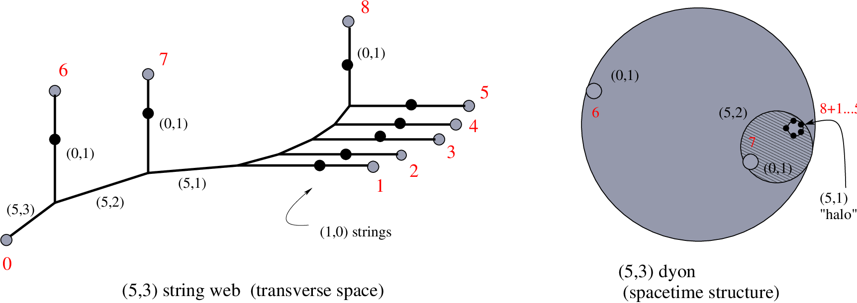
Finally, let us compare the core sizes with the core separations of relevance, to see the regimes of validity where the cores can be treated as pointlike and widely separated. From the equations (4.3), we get
| (40) |
For example, we have , i.e. center is pointlike (its inverse core size is much larger than its inverse separation from centers ) if . Similarly, the magnetic charges can be regarded as pointlike compared with their relative separations if certain conditions hold on the vevs: e.g. i.e. charge is pointlike if , while if , i.e. the point lies far above the line with slope (corresponding to the string). Likewise for charge to be pointlike, we have if , while if (which implies the earlier condition). These conditions are compatible and give a region in moduli space where this molecular structure of the configuration is reliable.
From Figure 4, we see that the limit (which through the constraint (39) implies ) corresponds to the various lines of marginal stability (i.e. the various string junction locations) coinciding. In this limit, the inverse core separations (4.3) all vanish, so that all charges are widely separated and the bound state unbinds. Keeping fixed in this limit ensures that the individual constituents with charges
| (41) |
are all pointlike to arbitrary accuracy, their core sizes using (40) in this limit being
| (42) |
As we move away from this region, e.g. as grow relative to the other vevs, the different centers begin to coalesce and their spatial separations cannot be distinguished clearly enough from their core sizes and the structure becomes fuzzy. Finally for large , we see the single dyon center . Clearly there exist different regions of moduli space where the can break up into different constituents. For instance, consider the region in moduli space
| (43) |
where branes- and separately branes- coincide. Now the dyon can break up into four constituents resulting in an effectively string web e.g. , where the and legs end on branes- and - respectively, while the leg ends on brane-. The internal structure of the dyon in this region can be analyzed by considering the appropriate limits in (4.3), resulting in a 3-center bound state configuration somewhat similar to the dyons described earlier.
5 More on internal structure transitions: string webs with internal faces
It is known that there are moduli in string webs corresponding to internal faces opening up (see e.g. [2, 10, 24]). We will consider what is perhaps the simplest such string web in SYM theory (left side of Figure 5). As can be seen from the Figure, the internal face opening up has internal string legs corresponding to strings.
We would like to understand the spacetime structure of the dyon in SYM theory that corresponds to such a web with an internal face. Towards this end, we see that the field configuration
| (44) |
is a description of the web with internal faces (middle of Figure 5). This configuration consists of three 3-pronged string web configurations, of charges , one pair from each of branes-, glued pairwise at appropriate charge cores. To elaborate, the spike from core in prong- glues onto that from in prong-, while the -spike in prong- glues onto that from in prong-. Finally the -spikes from prongs- glue onto each other. Alternatively, one could imagine branes- to have charge cores respectively. Consistency of the prong-gluing then forces , , and .

With the leg lying parallel to the -axis, , and scalar boundary conditions
| (45) |
it is straightforward to work out the core separations from the resulting constraint equations for the moduli as in our previous discussions, and we find
| (46) |
with corresponding core sizes, being the modulus corresponding to changing the size of the internal face. We see that the core separations can be tuned independently showing the three lines of marginal stability. In the limit , i.e. short web legs, all core separations diverge and we obtain pointlike widely separated cores, and a reliable field configuration. Unlike the 3-center configurations in Sec. 4.1, all core separations here are fixed and we have a rigid “molecule” of three constituent “atoms”, shaped like an isosceles triangle, with sides , for . When the internal face is of maximal size, i.e. zero size external web legs, we have (and corresponding other edge locations, e.g. ): then we have and infinite, showing for a physical dyon configuration corresponding to a maximal size face. This then shows that the triangle inequality for the 3-center configuration is always satisfied and the molecule shape does not degenerate.
This configuration and the string web then show that the dyon has asymptotic charges and three individual constituent cores of charge
| (47) |
Thus each internal leg corresponds to a charge core. By comparison, we see that the dyon for the same web but without the internal face corresponds to a 2-center configuration whose constituent cores have charges
| (48) |
the corresponding scalar field configuration (with brane- near LMS) being
| (49) |
the prong- gluing onto spikes- at the black circles shown on the left side of Figure 5.
Thus we see that the spacetime description of the opening up of the internal face is essentially similar to the kinds of transitions in internal structure that we saw earlier in Sec. 3. However, in this case, we are not moving around in the moduli space of the D-branes defining the vacuum: the D-brane locations are fixed. Changing moduli of the internal structure gives rise to charge rearrangement of the cores. Specifically we go to the symmetric point in moduli space of the 2-core configuration (mentioned at the end of Sec. 2) which effectively has a single coalesced core: this then breaks up into the 3-core configuration with rearranged charges.
The way the brane prong configurations glue onto each other is shown in Figure 5 (the thickened webs on the bottom), the black circles being the gluing locations (the grey circles corresponding to D-brane locations are not shown explicitly). A noteworthy point is that this system exhibits change in topology of the branes’ collective worldvolume 3-surface. With no internal face, we have the 3-dimensional analog of a genus-0 surface (5), while the opening up of the internal face creates a new “handle” in the interior of the brane 3-surface (5). This “tearing” of the 3-surface as we transit from no handle to one handle would seem like a singular process from the point of view of classical geometry, but we have to remember that our abelian approximations are not good in this intermediate region. The process of separation of the new cores from the single “effective” core involves the light nonabelian fields that we have neglected. We expect that the full nonabelian theory gives a smooth description of this brane prong topology change as the internal face opens up.
It is possible to describe webs with multiple internal faces along these lines. The right side of Figure 5 shows the web , with two internal faces opened up. We can construct a field configuration for this system by considering the two branes with legs to have a 4-pronged web scalar configuration each (of the sort described earlier in Sec. 4), and the brane with leg to be a 3-pronged web. These then glue onto each other (at the black circles) as shown in the Figure.
6 Discussion
We have described field configurations in an abelian approximation that describe dyons and their approximate internal structure in super Yang-Mills theory. These dovetail closely with string web configurations corresponding to the dyon states in D-brane constructions of these gauge theories. The internal structure of the dyon for fixed asymptotic charges is a complicated function of the moduli space in general, as we have seen, closely intertwining with the geometry of the corresponding string web in transverse space.
One could now ask how reliable these constructions are, in terms of giving insight into the dyon internal structure. Note that while the dyon/web is truly -BPS, the generic such state in a higher rank theory is not, for the following reason66 6 This arose in discussions with Ashoke Sen.. Recall that the BPS bound equations follow from restricting to a 2-dimensional subspace of the 6N-dimensional Coulomb branch: this corresponds to the fact that the generic string web is a planar configuration stretched between D-branes. This is crucial to having -th supersymmetry preserved. However a small perturbation to the locations of one or more of the D-branes will tilt the string web which will now no longer be planar: from the field theory point of view per se, this means one of the other transverse scalars has been turned on, ruining the Bogomolny bound in the energy functional. Thus the dyon/web is no longer precisely -BPS, with the exception being (since 3 points always lie on some plane)77 7 See e.g. [27, 26, 28] for some related discussions on lines of marginal stability in string theories..
From the field theory point of view, we have charge centers, held together in equilibrium by force balance (approximately, since some of the core separations are not determined by the methods here). In the regions of moduli space we have focussed on, i.e. near one or more lines of marginal stability, the charge cores are all effectively pointlike and widely separated. Thus it seems reasonable to suppose that the internal structure in spacetime that we have obtained here is in fact not drastically altered even though the dyon/web is not truly -BPS, at least at weak coupling. Essentially any such dyon is approximately a classical object in this regime, being a molecule-like configuration of widely separated pointlike charge cores, so that quantum corrections would seem to make negligible contributions to the force balance conditions. This corroborates with the fact that at weak string coupling, the string web is a relatively light object stretched between heavy D3-branes. Perhaps this makes the picture here more interesting since we seem to be describing approximate configurations, robust under small perturbations, for highly nontrivial non-supersymmetric bound states in super Yang-Mills theories of high rank. It would be very interesting to go beyond the abelian approximation here, perhaps by adding higher derivative terms to the effective action, or by considering the corresponding configurations in the full nonabelian theory.
As we have seen, the boundary conditions on the scalar moduli generically fix the electric-magnetic core separations, or more generally, those of constituents with mutually nonlocal charges. However the separations of mutually local charges are not fixed, so these must be regarded as moduli of the configurations. Thus the low energy dynamics of these dyons would be captured by an appropriate approximately supersymmetric quantum mechanics on the moduli space of these solutions. There presumably are similar moduli for dyon states that do not satisfy prime: in this case, some constituent cores would perhaps fragment. A systematic study, possibly equipped with a better understanding of the coupling dependence of these configurations, might draw connections to the quiver quantum mechanics of [20].
Finally, it would be interesting to understand black hole bound state configurations, in part along the lines described in [19, 20], and more recently [21, 26, 28] (see also e.g. the review [29]), and contrast them with the description of SYM dyons here. For instance, away from a line of marginal stability, we have seen that the SYM dyon centers here begin to coalesce, and nonabelian modes (i.e. the ultraviolet completion of the abelian approximation) become important. It would be interesting to understand if similar ultraviolet completions, i.e. stringy corrections to the low energy gravity description, are required for a careful understanding of the internal structure of black hole bound states away from lines of marginal stability (which would naively seem to involve merging or bifurcation of horizons). On a more technical note, perhaps some of these spacetime configurations for dyons corresponding to webs with internal faces might be of relevance for understanding black holes in Type IIB compactifications on , via effective string webs wrapped on corresponding to higher genus surfaces [25, 26].
More generally, this approach would perhaps closely tie into the broad ideas and attempts to understand black holes by decomposing it into constituent bits [30].
Acknowledgements: It is a pleasure to thank Frederik Denef and Ashoke Sen for discussions at the early stages and towards the completion of this work respectively. I have also benefitted from discussions with Atish Dabholkar and Suresh Nampuri on analyzing the degeneracies of Stern-Yi string web states from a string theory point of view. I’d like to thank the Organizers of the “From Strings to the LHC: II” school+conference, Bangalore, India, for hospitality during the final stages of this work.
Appendix A BPS bounds, brane prongs and string webs
Here we review the BPS state construction [12, 13] of string webs from the low energy effective action on the Coulomb branch, making perhaps slightly more manifest the brane prong description, paving the way for the configurations described in this paper. First, we consider an theory ( being electric, magnetic fields) with two scalars representing a 2-dim. subspace of the 6-dim. Coulomb branch. With a view to finding BPS solutions, we complete squares in the energy functional to obtain Bogomolny bound equations: this gives
| (50) |
where the boundaries are spheres around each of several charge cores in the system and one sphere at infinity, and we have used the divergence-free equations for the electric and magnetic fields away from the cores88 8 A similar Bogomolny bound in a nonabelian gauge theory would contain e.g. a BPS ’t Hooft-Polyakov monopole solution, with the nonabelian modes dying out exponentially outside the monopole core whose size is set by the Higgs vev. The abelian description here can be regarded as the approximate Dirac-monopole-like (semiclassical) description outside the charge core.. Labelling the boundaries so that the boundary is the one at infinity and the are the ones around the charge cores, within the abelian approximation, the scalars can be regarded as taking constant values at the -th boundary while at infinity they take their asymptotic vacuum values, say . This reduces the boundary terms to expressions involving the electric/magnetic charges , of the various cores. By charge conservation, the charges at infinity are . Then the BPS saturated mass (using in 4-dim)
| (51) |
(implied sum over the charge cores) arising from the boundary terms, is obtained when the BPS bound equations
| (52) |
hold, where we maximize w.r.t. , i.e. when
| (53) |
The scalars are harmonic, i.e. . Let us illustrate this with a few examples. A single charge core has , where are the units of electric and magnetic charge. A unit electric charge , is then given by
| (54) |
where we have chosen (which also satisfies (53)) so that the spike stretches along increasing . This is a -BPS state. Here we have set , i.e. we have turned off the scalar. Alternatively we have performed a rotation in the -plane so that the -string emanating from a D-brane stretches along the -axis. The factors are not important for our analysis, so we will drop this for convenience.
Now consider a 2-center configuration with , i.e. one charge core is purely electric while the other is purely magnetic. This is a -BPS state. This gives
| (55) |
where we have imposed boundary conditions so that the moduli values at the charge cores are , for simplicity. Now we see that if . Choosing , we have , giving the scalar field configurations
| (56) |
the constants of integration being fixed to be the vacuum moduli values. Effectively, our choice of has fixed our freedom to perform a rotation in the -plane, and ensured that e.g. electric charges correspond to F-strings stretched along the -axis, and more generally an charge corresponds to an -string stretched along a line of slope in the -plane.
The scalar configurations can now be interpreted as brane prongs approximating a string web with increasing accuracy as we approach the line of marginal stability, which lies at with our choices of moduli values.
Now let us go to higher rank theories. We expect on physical grounds that the theory above is UV incomplete, and must be regarded as a piece of a theory, arising as the Higgsed approximation to a theory. The energy functional for the theory is
| (57) |
Extremizing this and finding BPS states is straightforward but not simple. For the theory, details appear in [12, 13]. We will simply describe some intuitive aspects of the embedding of the brane-prong configurations into and theories: this should pave the way for the description of dyon-web configurations in the text.
We expect that a brane-spike representing a single charge must be patched up with a corresponding spike from another brane, the two spikes together being thought of as a low energy approximation to the full nonabelian theory. Thus for, say, a unit electric charge represented by a -string stretched between two D-branes at say and on the -plane, we expect the BPS bound equations
| (58) |
from the two D-branes separately, giving the scalar field configurations (2). For the two spikes to be glued together, we require that the two cores be located at the same position along the D-brane worldvolume directions and the core sizes be the same (within this approximation). This implies that the gluing happens at the midpoint of the line joining the two branes, i.e. at the singularity corresponding to enhanced gauge symmetry on the moduli space. Note that the gluing and charge boundary conditions are consistent with the fact that the brane appears to have a positive charge flux emanating from the gluing core, while the brane appears to have a negative charge flux emanating from the gluing location.
Similarly, the brane-prong configuration (56) representing say the string web in the theory must be patched up with corresponding spikes/prongs from two other branes, the three spike/prong pieces together being thought of as a low energy approximation to the full nonabelian theory. Thus for, say, the string web stretched between three D-branes at say on the -plane (Figure 1), we expect the BPS bound equations
| (59) |
The expectation that the electric part of prong-0 glues onto that of brane-1 while the magnetic part of prong-0 glues onto that of brane-2 implies
| (60) |
These field strengths alongwith the BPS bound equations imply the scalar field configurations in (2.1).
It is similarly possible to write out educated guesses for the BPS bound equations for the higher rank/charge cases and thence the corresponding field configurations: e.g. the BPS bound equations for the state described in the text are
| (61) |
from which we can write the scalar field configurations (4) specializing to the state.
The field configurations in the text are written with a rotation in the transverse -plane, as for the single theory described earlier, so that the dyon spike from brane- (away from any line of marginal stability) points in the direction.
References
- [1] O. Bergman, “Three-pronged strings and 1/4 BPS states in N = 4 super-Yang-Mills theory,” Nucl. Phys. B 525, 104 (1998) [arXiv:hep-th/9712211].
- [2] O. Bergman and B. Kol, “String webs and 1/4 BPS monopoles,” Nucl. Phys. B 536, 149 (1998) [arXiv:hep-th/9804160].
- [3] K. Hashimoto, H. Hata and N. Sasakura, “3-string junction and BPS saturated solutions in SU(3) supersymmetric Yang-Mills theory,” Phys. Lett. B 431, 303 (1998) [arXiv:hep-th/9803127].
- [4] T. Kawano and K. Okuyama, “String network and 1/4 BPS states in N = 4 SU(N) supersymmetric Yang-Mills theory,” Phys. Lett. B 432, 338 (1998) [arXiv:hep-th/9804139].
- [5] K. M. Lee and P. Yi, “Dyons in N = 4 supersymmetric theories and three-pronged strings,” Phys. Rev. D 58, 066005 (1998) [arXiv:hep-th/9804174].
- [6] D. Bak, K. Hashimoto, B. H. Lee, H. Min and N. Sasakura, “Moduli space dimensions of multi-pronged strings,” Phys. Rev. D 60, 046005 (1999) [arXiv:hep-th/9901107]; D. Bak, C. k. Lee, K. M. Lee and P. Yi, “Low energy dynamics for 1/4 BPS dyons,” Phys. Rev. D 61, 025001 (2000) [arXiv:hep-th/9906119]; D. Bak, K. M. Lee and P. Yi, “Quantum 1/4 BPS dyons,” Phys. Rev. D 61, 045003 (2000) [arXiv:hep-th/9907090]; D. Bak and K. M. Lee, “Comments on the moduli dynamics of 1/4 BPS dyons,” Phys. Lett. B 468, 76 (1999) [arXiv:hep-th/9909035].
- [7] M. Stern and P. Yi, “Counting Yang-Mills dyons with index theorems,” Phys. Rev. D 62, 125006 (2000) [arXiv:hep-th/0005275].
- [8] C. G. . Callan and J. M. Maldacena, “Brane dynamics from the Born-Infeld action,” Nucl. Phys. B 513, 198 (1998) [arXiv:hep-th/9708147].
- [9] J. P. Gauntlett, C. Koehl, D. Mateos, P. K. Townsend and M. Zamaklar, “Finite energy Dirac-Born-Infeld monopoles and string junctions,” Phys. Rev. D 60, 045004 (1999) [arXiv:hep-th/9903156].
- [10] B. Kol and M. Kroyter, “On the spatial structure of monopoles,” arXiv:hep-th/0002118.
- [11] A. Ritz, M. A. Shifman, A. I. Vainshtein and M. B. Voloshin, “Marginal stability and the metamorphosis of BPS states,” Phys. Rev. D 63, 065018 (2001) [arXiv:hep-th/0006028].
- [12] P. C. Argyres and K. Narayan, “String webs from field theory,” JHEP 0103, 047 (2001) [arXiv:hep-th/0101114].
- [13] P. C. Argyres and K. Narayan, “String webs and the decay of supersymmetric particles,” Int. J. Mod. Phys. A 16S1C, 962 (2001) [arXiv:hep-th/0101139].
- [14] A. Ritz and A. I. Vainshtein, “Long range forces and supersymmetric bound states,” Nucl. Phys. B 617, 43 (2001) [arXiv:hep-th/0102121].
- [15] E. Weinberg, P. Yi, “Magnetic Monopole Dynamics, Supersymmetry, and Duality”, Phys. Rept. 438, 65 (2007), [hep-th/0609055].
- [16] J. H. Schwarz, “Lectures on Superstring and M Theory Dualities”, Nuc. Phys. Proc. Suppl. B55 1 (1997) [hep-th/9607201].
- [17] K. Dasgupta and S. Mukhi, “BPS nature of 3-string junctions,” Phys. Lett. B 423, 261 (1998) [arXiv:hep-th/9711094].
- [18] A. Sen, “String network,” JHEP 9803, 005 (1998) [arXiv:hep-th/9711130].
- [19] F. Denef, “Supergravity flows and D-brane stability,” JHEP 0008, 050 (2000) [arXiv:hep-th/0005049]; F. Denef, B. R. Greene and M. Raugas, “Split attractor flows and the spectrum of BPS D-branes on the quintic,” JHEP 0105, 012 (2001) [arXiv:hep-th/0101135]. B. Bates, F. Denef, “Exact solutions for supersymmetric stationary black hole composites”, [hep-th/0304094].
- [20] F. Denef, “Quantum quivers and Hall/hole halos,” JHEP 0210, 023 (2002) [arXiv:hep-th/0206072].
- [21] F. Denef, G. Moore, “Split states, entropy enigmas, holes and halos”, [arXiv:hep-th/0702146].
- [22] N. Seiberg, E. Witten, “Electric-magnetic duality, monopole condensation, and confinement in supersymmetric Yang-Mills theory”, [hep-th/9407087].
- [23] A. Sen, “F-theory and orientifolds”, [hep-th/9605150]; T. Banks, M. Douglas, N. Seiberg, “Probing F-theory with branes”, [hep-th/9605199]; A. Sen, “BPS states on a three-brane probe”, [hep-th/9608005].
- [24] P. Shockley, L. Thorlacius, “Zero mode dynamics of string webs”, [hep-th/0101080].
- [25] D. Gaiotto, “Re-recounting dyons in string theory”, [hep-th/0506249].
- [26] A. Dabholkar, D. Gaiotto, S. Nampuri, “Comments on the spectrum of CHL dyons”, [hep-th/0702150].
- [27] A. Sen, “Walls of marginal stability and dyon spectrum in supersymmetric string theories”, [hep-th/0702141]; “ Rare decay modes of quarter BPS dyons”, arXiv:0707.1563 [hep-th]; “ Three string junction and dyon spectrum”, arXiv:0708.3715 [hep-th]; M. Cheng, E. Verlinde, “Dying dyons don’t count”, arXiv:0706.2363 [hep-th]; A. Mukherjee, S. Mukhi, R. Nigam, “Dyon death eaters”, arXiv:0707.3035 [hep-th]; S. Banerjee, A. Sen, “Duality orbits, dyon spectrum and gauge theory limit of heterotic string theory on ”, arXiv:0712.0043 [hep-th];
- [28] A. Sen, “Two centered black holes and dyon spectrum”, arXiv:0705.3874 [hep-th].
- [29] A. Sen, “Black hole entropy function, attractors and precision counting of microstates”, arXiv:0708.1270 [hep-th].
- [30] R. Britto-Pacumio, J. Michelson, A. Strominger, A. Volovich, “Lectures on superconformal quantum mechanics and multi-black hole moduli spaces”, [hep-th/9911066]; S. D. Mathur, “The fuzzball proposal for black holes: An elementary review”, [hep-th/0502050].