Cardiac Alternans Arising from an Unfolded Border-Collision Bifurcation

Cardiovascular disease is the number one cause of death in the United States [1]. Over half of the mortality is due to sudden cardiac arrest that is often initiated by ventricular fibrillation, a fatal heart rhythm disorder. The induction and maintenance of ventricular fibrillation has been connected to the dynamics of local cardiac electrical properties [2, 3]. Therefore, studying cardiac dynamics is important for understanding life-threatening arrhythmias and developing therapies for preventing sudden cardiac death.

To develop an understanding of cardiac rhythm instability, we briefly review the electrophysiology of the heart. Cardiac cells respond to an electrical stimulus by eliciting an action potential [4], which consists of a rapid depolarization of the transmembrane voltage followed by a much slower repolarization process before returning to the resting value (Fig. 1). The time interval during which the voltage is elevated is called the action potential duration (APD). As shown in Fig. 1, the time between the end of an action potential to the beginning of the next one is called the diastolic interval (DI). The time interval between two consecutive stimuli is called the basic cycle length (BCL).

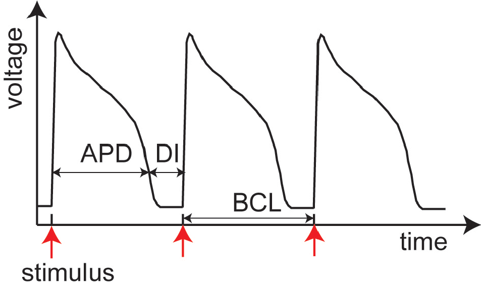
Under a periodic train of electrical stimuli, the steady-state response consists of phase-locked action potentials, where each stimulus gives rise to an identical action potential (1:1 pattern) when the pacing rate is slow. When the pacing rate becomes sufficiently fast, the 1:1 pattern may be replaced by a 2:2 pattern, so-called electrical alternans [5, 6, 7], where the APD alternates between short and long values. Using theory and experiments, a causal connection between alternans and the vulnerability to fatal cardiac arrhythmias such as ventricular fibrillation has been established by various authors [2, 3, 5-13]. Therefore, understanding mechanism of alternans is a crucial step in detection and prevention of fatal arrhythmias.

It has long been hypothesized [8, 9, 10, 11, 12, 13] that alternans is mediated by a classical period-doubling bifurcation, which can be described using a smooth iterated map, and which occurs when one eigenvalue of the Jacobian crosses the unit circle through $-1$ [14, 15]. We restrict our attention to supercritical rather than subcritical bifurcations because the former are observed in most experiments and theoretical models exhibiting electrical alternans. Based on this hypothesis, various authors attempted to develop criteria for the onset of alternans [8, 11, 10] as well as algorithms to control alternans [11, 12, 13]. Recently, a few authors [16, 17, 18, 19, 20] proposed a different hypothesis: alternans may be mediated through a border-collision period-doubling bifurcation. Border-collision bifurcations occur in piecewise smooth maps [21, 22]. In contrast to classical period-doubling bifurcations, eigenvalues are not indicative of the onset of a border-collision period-doubling bifurcation. Instead, a border-collision bifurcation occurs when a branch of fixed points collides with a border, i.e., a discontinuity surface in state space. Knowing the mechanism of alternans may help researchers to choose the proper types of functions to model this instability. More importantly, to develop model-based control methods requires knowledge of the underlying dynamics [17].

The aforementioned intrinsic differences between the two bifurcation types lead to differences in their bifurcation diagrams, as depicted in Fig. 2. Here, the two bifurcated branches of a smooth period-doubling bifurcation become tangent to each other at the bifurcation point, while the bifurcated branches of a border-collision bifurcation open at an angle. Thus, in principle the bifurcation diagrams should distinguish between the two bifurcation types. However, in practice, experiments can provide only a limited number of measurements (especially in biological systems), so the resulting bifurcation diagrams do not have sufficient resolution. This is illustrated in Fig. 2, where the discrete points representing experimental data along a bifurcation diagram do not readily reveal the true type of bifurcation. Therefore, there is a need for a more sensitive technique to differentiate between the two bifurcations.

Based on prebifurcation amplification, our group has developed a robust technique to distinguish between smooth and border-collision bifurcations [27-30]. Here, we briefly review the results. It has been shown theoretically and experimentally that, near the onset of a smooth period-doubling bifurcation, subharmonic perturbations in a bifurcation parameter result in amplified disturbances in the response, a phenomenon known as prebifurcation amplification [23, 24, 25, 26]. In the following, we will show that, under variations in system parameters, prebifurcation amplification exhibits qualitatively different scaling laws in border-collision period-doubling and smooth period-doubling bifurcations. Thus, prebifurcation amplification is a useful technique to distinguish between the two possible types of period-doubling bifurcations.

To illustrate the concept of prebifurcation amplification, we consider a dynamical system described by the following map

$$x_{n+1}=f\left(x_{n};B\right),$$

(1)

where $B$ represents a bifurcation parameter, e.g., the BCL in cardiac models. Both the function $f$ and state variable $x$ may be one- or multi-dimensional. Let us assume that, at a critical value $B=B_{\text{bif}}$, the system undergoes a period-doubling bifurcation that is either a smooth type for smooth $f$ [14, 15] or a border-collision type for piecewise smooth $f$ [21, 22]. We further assume that the stable period-one solution lies on the side $B>B_{\text{bif}}$, as indicated in Fig. 2.

When a subharmonic perturbation is applied to $B$ under conditions when $B>B_{\text{bif}}$, it renders map (1) as

$$x_{n+1}=f\left(x_{n};B+\left(-1\right)^{n}\delta\right),$$

(2)

where $\delta$ is the amplitude of the perturbation. The perturbation may also be imposed in the form of $B-\left(-1\right)^{n}\delta$, which leads to a solution only different in phase from that of Eqn. (2). Since $B$ represents the pacing interval in cardiac models, such a variation in $B$ is referred to as alternate pacing. For $B$ greater than but close to $B_{\text{bif}}$ and small $\delta$, the steady-state response of Eqn. (2) consists of alternating recurrent states of $x_{\text{even}}$ and $x_{\text{odd}}$, which satisfy the following conditions

	$\displaystyle x_{\text{even}}$	$\displaystyle=f\left(x_{\text{odd}};B-\delta\right),$		(3)
	$\displaystyle x_{\text{odd}}$	$\displaystyle=f\left(x_{\text{even}};B+\delta\right).$		(4)

In cardiac models, one component of the vector $x$ is the APD, henceforth denoted by $A$. Alternate pacing of these models results in a long-short beat-to-beat variation in pacing intervals, which in turns cause alternation in $A$ even when $B>B_{\text{bif}}$. Since a period-doubling bifurcation is sensitive to subharmonic perturbations, perturbations in $B$ result in amplified disturbances in $A$. The effect of prebifurcation amplification can then be characterized by a gain defined as follows

$$\text{$\Gamma$}\equiv\frac{\left|A_{\text{even}}-A_{\text{odd}}\right|}{2\delta}.$$

(5)

To identify the bifurcation mechanism mediating cardiac alternans, we implemented the aforementioned technique in paced in vitro bullfrog heart [30, 31], where the experiments reveal a novel phenomenon that cannot be explained by the above simple dichotomy of smooth/nonsmooth bifurcations. Specifically, our experiments show that very close to the bifurcation point, $\Gamma$ decreases with $\delta$, which agrees with the smooth bifurcation (Fig. 3b), whereas further away $\Gamma$ increases with $\delta$, which agrees with the border-collision bifurcation (Fig. 3d). A bifurcation that exibits such a crossover between smooth and border-collision behaviors is named a hybrid period-doubling bifurcation [30, 31]. We further found that the essence of this hybrid behavior can be reproduced by a model of a so-called unfolded border-collision bifurcation. In the remainder of this paper, we will carry out a detailed analysis of the unfolded border-collision model. This analysis will help to understand the mathematical mechanism underlying the crossover between smooth and nonsmooth behaviors, providing guidance for the development of future models.

To study the prebifurcation amplification of map (12), we apply an alternating perturbation to the BCL’s; in symbol, $B_{n}=B+\left(-1\right)^{n}\delta$, where $B$ is a baseline BCL and $\delta$ is a small but nonzero perturbation. Under this alternate pacing, it follows that $D_{n}=B+\left(-1\right)^{n}\delta-A_{n}$. Here, we require that $B>B_{\text{bif}}$ because prebifurcation dynamics is of interest. Denoting the steady-state APDs under alternate pacing by $A_{\text{even}}$ and $A_{\text{odd}}$, it follows from Eqn. (12) that

	$\displaystyle A_{\text{even}}$	$\displaystyle=A_{\text{c}}+\alpha\left(D_{\text{odd}}-D_{\text{th}}\right)+\beta\sqrt{\left(D_{\text{odd}}-D_{\text{th}}\right)^{2}+D_{\text{s}}^{2}},$		(19)
	$\displaystyle A_{\text{odd}}$	$\displaystyle=A_{\text{c}}+\alpha\left(D_{\text{even}}-D_{\text{th}}\right)+\beta\sqrt{\left(D_{\text{even}}-D_{\text{th}}\right)^{2}+D_{\text{s}}^{2}},$		(20)

where

	$\displaystyle D_{\text{odd}}$	$\displaystyle=B-\delta-A_{\text{odd}},$		(21)
	$\displaystyle D_{\text{even}}$	$\displaystyle=B+\delta-A_{\text{even}}.$		(22)

For later convenience, we let

$$B=B_{c}+\Delta B=A_{\text{c}}+D_{\text{th}}+\Delta B$$

(23)

and we define $\Delta_{\text{even}}$ and $\Delta_{\text{odd}}$ by

$$A_{\text{even}}=\Delta_{\text{even}}+A_{\text{c}}\text{\thinspace\ \ and }\ A_{\text{odd}}=\Delta_{\text{odd}}+A_{\text{c}}.$$

(24)

Substituting the above equations into Eqns. (19) and (20) yields

	$\displaystyle\Delta_{\text{even}}+\alpha\,\left(\Delta_{\text{odd}}+\delta-\Delta B\right)$	$\displaystyle=\beta\sqrt{\left(\Delta_{\text{odd}}+\delta-\Delta B\right)^{2}+D_{\text{s}}^{2}},$		(25)
	$\displaystyle\Delta_{\text{odd}}+\alpha\,\left(\Delta_{\text{even}}-\delta-\Delta B\right)$	$\displaystyle=\beta\sqrt{\left(\Delta_{\text{even}}-\delta-\Delta B\right)^{2}+D_{\text{s}}^{2}}.$		(26)

One can then show that

		$\displaystyle\left(\left(1-\alpha\right)\left(\Delta_{\text{even}}-\Delta_{\text{odd}}\right)+2\,\alpha\,\delta\right)\left(\left(1+\alpha\right)\left(\Delta_{\text{even}}-\Delta_{\text{odd}}\right)-2\,\alpha\,\Delta B\right)$
		$\displaystyle=\beta^{2}\left(\Delta_{\text{odd}}-\Delta_{\text{even}}+2\,\delta\right)\left(\Delta_{\text{odd}}+\Delta_{\text{even}}-2\,\Delta B\right)$		(27)

Let

$$\gamma=\frac{\Delta_{\text{even}}-\Delta_{\text{odd}}}{2\,\delta};$$

(28)

i.e., $\gamma$ is a gain-like quantity that can be either positive or negative (cf. 5). Substituting the definition of $\gamma$ into Eqn. (27) yields

		$\displaystyle 2\,\delta\left(\left(1-\alpha\right)\gamma+\alpha\right)\left(\left(1+\alpha\right)\left(\Delta_{\text{even}}-\Delta_{\text{odd}}\right)-2\,\alpha\,\Delta B\right)$
		$\displaystyle=2\delta\,\beta^{2}\left(1-\gamma\right)\left(\Delta_{\text{odd}}+\Delta_{\text{even}}-2\,\Delta B\right).$		(29)

Because we consider nonzero $\delta$, Eqn. (29) can be reduced to

$$\gamma\left(c_{1}\Delta B+d_{1}\left(\Delta_{\text{even}}+\Delta_{\text{odd}}\right)\right)=c_{2}\Delta B+d_{2}\left(\Delta_{\text{even}}+\Delta_{\text{odd}}\right),$$

(30)

where

	$\displaystyle c_{1}$	$\displaystyle=-2\left(\beta^{2}+\alpha\left(1-\alpha\right)\right),$		(31)
	$\displaystyle d_{1}$	$\displaystyle=1-\alpha^{2}+\beta^{2},$		(32)
	$\displaystyle c_{2}$	$\displaystyle=2\left(\alpha^{2}-\beta^{2}\right),$		(33)
	$\displaystyle d_{2}$	$\displaystyle=-\left(\alpha\left(1+\alpha\right)-\beta^{2}\right).$		(34)

It then follows that

$$\gamma=\frac{c_{2}\Delta B+d_{2}\left(\Delta_{\text{even}}+\Delta_{\text{odd}}\right)}{c_{1}\Delta B+d_{1}\left(\Delta_{\text{even}}+\Delta_{\text{odd}}\right)}.$$

(35)

Since $\Delta_{\text{even}}$ and $\Delta_{\text{odd}}$ depend on $\Delta B$ and $\delta$, $\gamma$ is a function of $\Delta B$ and $\delta$.

Recalling definition (5), we find the prebifurcation amplification gain as

$$\Gamma=\left|\frac{c_{2}\Delta B+d_{2}\left(\Delta_{\text{even}}+\Delta_{\text{odd}}\right)}{c_{1}\Delta B+d_{1}\left(\Delta_{\text{even}}+\Delta_{\text{odd}}\right)}\right|.$$

(36)

Particularly, when $\Delta B=0$, i.e. $B=B_{\text{c}}=A_{\text{c}}+D_{\text{th}}$, the gain is

$$\Gamma=\left|\frac{d_{2}}{d_{1}}\right|=\frac{\alpha+\left(\alpha^{2}-\beta^{2}\right)}{1-\left(\alpha^{2}-\beta^{2}\right)}.$$

(37)

Therefore, when $B=B_{c}$, $\Gamma$ is same for all $\delta$. With some manipulation, one can show that $\partial\Gamma/\partial B\neq 0$ at $B=B_{c}$. Moreover, when $B$ is sufficiently close to $B_{\text{bif}}<B_{c}$ and $\delta$ is fixed, $\Gamma$ decreases as $B$ increases as described in previous section and proven in [28]. Thus, for a given $\delta$, $\Gamma$ is a monotonically decreasing function of $B$ and $\Gamma$ becomes constant at $B=B_{c}$. Because $\Gamma$ is a monotonically decreasing function of $\delta$ when $B\gtrsim B_{\text{bif}}$, as shown in the previous section (see also [28]), it follows by continuity that $\Gamma$ will increase as $\delta$ increases in the region of $B>B_{c}$. In other words, the map (12) exhibits smooth like behavior when $B$ is sufficiently close to $B_{\text{bif}}$ and border-collision like behavior when $B>B_{c}$ (see the relation between $B_{\text{bif}}$ and $B_{\text{c}}$ in Fig. 4).

Before comparing the proposed model to experimental data, we review the class of models that are most commonly used in the cardiac research community. These models relate APD and DI through exponential functions. Typically, parameters of a model are obtained by fitting the model to the so-called dynamic restitution curve, which is a plot of the steady-state APD vs. DI. For example, in their pioneering work, Guevara et al. [32] proposed a model of cardiac dynamics as

$$A_{n+1}=201-98\,e^{-D_{n}/43}-35\,e^{-D_{n}/653},$$

(38)

where all variables and parameters have the unit of millisecond. Parameters of map (38) were obtained by fitting the dynamic restitution curve measured in experiments performed on quiescent aggregates of ventricular cells from 7-day-old embryonic chick hearts [32]. Although the model of Guevara et al. fits the dynamic restitution curve reasonably well (Fig. 5, top panel), it does not accurately describe the response beyond the bifurcation to alternans, as is evident from the bifurcation diagram of steady-state APD vs. BCL (Fig. 5, bottom panel). A careful examination reveals that the dynamic restitution curve is well approximated by two distinct parts with significantly different slopes. The transition between the two slopes occurs with a small interval near DI$\approx 60$ ms, which is also approximately where the transition to alternans occurs. Now, we recall that the unfolded border-collision model (12), with properly chosen parameters, describes such rapid changes between two distinct slopes. Fitting map (12) to the experimental dynamic restitution data, we obtain a set of parameters

	$$\displaystyle\alpha=0.69,\,\beta=-0.64,\,$$
	$$\displaystyle A_{\text{c}}=161\,\text{ms},\,D_{\text{th}}=62\,\text{ms,}\,\text{and}\ D_{\text{s}}=15\,\text{ms}.$$		(39)

As shown in Fig. 5, the unfolded border-collision map (12) with these parameters faithfully reproduces the bifurcation diagram, including the alternans branches. As demonstrated in Fig. 4, the bifurcation diagram of a border-collision map is close to that of its unfolded counterpart except near the bifurcation point. Thus, one expects a reasonable fit to the experimental data in Fig. 5 using a pure border-collision map, i.e., letting $D_{s}=0$. However, as has been established in the previous section, the nonsmooth map can not capture hybrid behaviors in the prebifurcation gain. Here, for clarity, the bifurcation diagram of the corresponding border-collision model is not shown in Fig. 5.

We then simulate map (12) with alternate pacing. Figure 6 shows $\Gamma$ vs. $B$ for different values of $\delta$. These curves cross one another at $B=B_{\text{c}}=223$ ms. Note that a period-doubling bifurcation occurs at $B=198$ ms. It is clear that $\Gamma$ vs. $\delta$ displays a trend consistent with a smooth bifurcation (cf. Fig. 3 (b)) when $B<B_{\text{c}}$ and, on the other hand, $\Gamma$ vs. $\delta$ shows a trend consistent with a border-collision bifurcation when $B>B_{\text{c}}$ (cf. Fig. 3 (d)). Since Guevara et al. did not perform alternate pacing experiments, no data are available for comparison. However, we note that the simulation here is in qualitative agreement with our previous experiments on bullfrog ventricles [30, 31].

Because $A_{\text{even}}>A_{\text{bif}}$ and $A_{\text{odd}}>A_{\text{bif}}$, it follows from Eqn. (43) that

	$\displaystyle A_{\text{even}}$	$\displaystyle=f_{1}\left(A_{\text{odd}};B-\delta\right),$		(46)
	$\displaystyle A_{\text{odd}}$	$\displaystyle=f_{1}\left(A_{\text{even}};B+\delta\right).$		(47)

To leading order, the solution of Eqs. (46) and (47) is

	$\displaystyle A_{\text{even}}$	$\displaystyle=A_{\text{bif}}+\frac{\partial_{B}f}{1-\partial_{A}f_{1}}\left(B-B_{\text{bif}}\right)-\frac{\partial_{B}f}{1+\partial_{A}f_{1}}\delta,$		(48)
	$\displaystyle A_{\text{odd}}$	$\displaystyle=A_{\text{bif}}+\frac{\partial_{B}f}{1-\partial_{A}f_{1}}\left(B-B_{\text{bif}}\right)+\frac{\partial_{B}f}{1+\partial_{A}f_{1}}\delta.$		(49)

Recalling the conditions in Eqs. (41) and (42), it follows that $A_{\text{odd}}>A_{\text{even}}$. Moreover, it follows from Eqn. (48) that the unilateral solution is valid as long as

$$B-B_{\text{bif}}>\rho_{\text{crit}}\,\delta,$$

(50)

where

$$\rho_{\text{crit}}=\frac{1-\partial_{A}f_{1}}{1+\partial_{A}f_{1}}>0\text{.}$$

(51)

The bilateral solution occurs in the region $B-B_{\text{bif}}<\rho_{\text{crit}}\,\delta$. By continuity, the solution in this region satisfies $A_{\text{odd}}>A_{\text{bif}}>A_{\text{even}}$. It follows from Eqn. (43) that

	$\displaystyle A_{\text{even}}$	$\displaystyle=f_{1}\left(A_{\text{odd}};B-\delta\right),$		(52)
	$\displaystyle A_{\text{odd}}$	$\displaystyle=f_{2}\left(A_{\text{even}};B+\delta\right).$		(53)

Linearizing Eqns. (52) and (53) around $A=A_{\text{bif}}$ and $B=B_{\text{bif}}$ yields

	$\displaystyle A_{\text{even}}$	$\displaystyle=A_{\text{bif}}+\partial_{A}f_{1}\ast\left(A_{\text{odd}}-A_{\text{bif}}\right)+\partial_{B}f\ast\left(B-B_{\text{bif}}-\delta\right),$		(54)
	$\displaystyle A_{\text{odd}}$	$\displaystyle=A_{\text{bif}}+\partial_{A}f_{2}\ast\left(A_{\text{even}}-A_{\text{bif}}\right)+\partial_{B}f\ast\left(B-B_{\text{bif}}+\delta\right),$		(55)

where the derivatives are evaluated at $\left(A_{\text{bif}};B_{\text{bif}}\right)$. Solving the above equations yields the leading-order solution for $A_{\text{even}}$ and $A_{\text{odd}}$ as

	$\displaystyle A_{\text{even}}$	$\displaystyle=A_{\text{bif}}+\frac{\left(1+\partial_{A}f_{1}\right)\left(B-B_{\text{bif}}\right)-\,\left(1-\partial_{A}f_{1}\right)\delta}{1-\partial_{A}f_{2}\,\partial_{A}f_{1}}\partial_{B}f,$		(56)
	$\displaystyle A_{\text{odd}}$	$\displaystyle=A_{\text{bif}}+\frac{\left(1+\partial_{A}f_{2}\right)\left(B-B_{\text{bif}}\right)+\left(1-\partial_{A}f_{2}\right)\delta}{1-\partial_{A}f_{2}\,\partial_{A}f_{1}}\partial_{B}f.$		(57)

When $B-B_{\text{bif}}>\rho_{\text{crit}}\,\delta$, it follows from Eqs. (48) and (49) that the gain is

$$\Gamma=\frac{A_{\text{odd}}-A_{\text{even}}}{2\,\delta}=\frac{\partial_{B}f}{1+\partial_{A}f_{1}}\equiv\Gamma_{\text{const}}.$$

(58)

When $B-B_{\text{bif}}<\rho_{\text{crit}}\,\delta$, it follows from Eqs. (56) and (57) that the gain is

	$\displaystyle\Gamma$	$\displaystyle=\frac{A_{\text{odd}}-A_{\text{even}}}{2\,\delta}$		(59)
		$\displaystyle=\Gamma_{\text{const}}-\gamma\left(\frac{B-B_{\text{bif}}}{\delta}-\rho_{\text{crit}}\right),$		(60)

where

$$\gamma=\frac{\partial_{A}f_{1}-\partial_{A}f_{2}}{2\left(1-\partial_{A}f_{2}\,\partial_{A}f_{1}\right)}\partial_{B}f>0.$$

(61)

References

- [1] http://www.americanheart.org/.
- [2] D.S. Rosenbaum, L.E. Jackson, J.M. Smith, H. Garan, J.N. Ruskin, and R.J. Cohen, ‘Electrical Alternans and Vulnerability to Ventricular Arrhythmias,’ New England Journal of Medicine, 330, 235-241, (1994).
- [3] J.M. Pastore, S.D. Girouard, K.R. Laurita, F.G. Akar, and D.S. Rosenbaum, ‘Mechanism Linking T-Wave Alternans to the Genesis of Cardiac Fibrillation,’ Circulation, 99, 1385-1394, (1999).
- [4] R. Plonsey and R.C. Barr, Bioelectricity: A Quantitative Approach (Kluwer, New York, 2000).
- [5] R.F. Gilmour Jr. and D.R. Chialvo, ‘Electrical Restitution, Critical Mass, and the Riddle of Fibrillation,’ Journal of Cardiovascular Electrophysiology, 10, 1087-1089, (1999).
- [6] Garfinkel, Y. H. Kim, O. Voroshilovsky, Z. Qu, J. R. Kil, M. H. Lee, H. S. Karagueuzian, J. N.Weiss, and P. S. Chen, ‘Preventing Ventricular Fibrillation by Flattening Cardiac Restitution’, Proceedings of the National Academy of Sciences of the United States of America, 97, 6061-6066, (2000).
- [7] A. Panfilov, ‘Spiral Breakup as a Model of Ventricular Fibrillation,’ Chaos, 8, 57-64, (1998).
- [8] J.B. Nolasco and R.W. Dahlen, ‘A Graphic Method for the Study of Alternation in Cardiac Action Potentials,’ Journal of Applied Physiology, 25, 191-196, (1968).
- [9] D.R. Chialvo, D.C. Michaels, and J. Jalife, ‘Supernormal Excitability as a Mechanism of Chaotic Dynamics of Activation in Cardiac Purkinje-Fibers,’ Circulation Research, 66, 525-545, (1990).
- [10] J.J. Fox, E. Bodenschatz, and R.F. Gilmour, ‘Period-doubling Instability and Memory in Cardiac Tissue,’ Physical Review Letters, 89, 138101 1-4, (2002).
- [11] G.M. Hall and D.J. Gauthier, ‘Experimental Control of Cardiac Muscle Alternans,’ Physical Review Letters, 88, 198102 1-4, (2002).
- [12] E.G. Tolkacheva, M.M. Romeo, M. Guerraty, and D.J. Gauthier, ‘Condition for Alternans and its Control in a Two-dimensional Mapping Model of Paced Cardiac Dynamics,’ Physical Review E, 69, 031904 1-8 (2004).
- [13] K. Hall, D.J. Christini, M. Tremblay, J.J. Collins, L. Glass, and J. Billette, ‘Dynamic Control of Cardiac Alternans,’ Physical Review Letters, 78, 4518-4521 (1997).
- [14] S.H. Strogatz, Nonlinear Dynamics and Chaos (Westview, Cambridge, 1994).
- [15] A.H. Nayfeh and B. Balachandran, Applied Nonlinear Dynamics (Wiley, New York, 1995).
- [16] J. Sun, F. Amellal, L. Glass, and J. Billette, ‘Alternans and Period-doubling Bifurcations in Atrioventricular Nodal Conduction,’ Journal of Theoretical Biology, 173, 79-91, (1995).
- [17] M.A. Hassouneh and E.H. Abed, ‘Border Collision Bifurcation Control of Cardiac Alternans,’ International Journal of Bifurcations and Chaos, 14, 3303-3315, (2004).
- [18] C.M. Berger, H. Dobrovolny, X. Zhao, D.G. Schaeffer, W. Krassowska, D.J. Gauthier, ‘Evidence for a Border-collision Bifurcation in Paced Cardiac Tissue,’ Southeastern Section of the APS, Gainesville, FL, November 10-12, 2005.
- [19] F. Fenton, ‘Beyond Slope One: Alternans Suppression and Other Understudied Properties of APD Restitution,’ KITP Miniprogram on Cardiac Dynamics, Kavli Institute for Theoretical Physics, Santa Barbara, CA, July 28, 2006
- [20] E.M. Cherry and F.H. Fenton, ‘A Tale of Two Dogs: Analyzing Two Models of Canine Ventricular Electrophysiology,’ American Journal of Physiology-Heart and Circulatory Physiology, 292: H43 - H55 (2007).
- [21] M. di Bernardo, C. Budd, A. Champneys, and P. Kowalczyk, Piecewise-Smooth Dynamical Systems: Theory and Applications, Springer, New York, 2007.
- [22] Z.T. Zhusubaliyev and E. Mosekilde, Bifurcations and Chaos in Piecewise-Smooth Dynamical Systems (World Scientific, Singapore, 2003).
- [23] K. Wiesenfeld, ‘Virtual Hopf Phenomenon: A New Precursor of Period-Doubling Bifurcations,’ Physical Review A, 32, 1744 (1985).
- [24] K. Wiesenfeld and B. McNamara, ‘Small-Signal Amplification in Bifurcating Dynamical Systems,’ Physical Review A, 33, 629-642 (1986); erratum: ibid 33, 3578 (1986).
- [25] Yu. A. Kravtsov and E.D. Surovyatkina, ‘Nonlinear Saturation of Prebifurcation Noise Amplification,’ Physics Letters A, 319, 348 (2003).
- [26] E.D. Surovyatkina, ‘Rise and Saturation of the Correlation Time near Bifurcation Threshold,’ Physics Letters A, 329, 169 (2004).
- [27] J. Heldstab, H. Thomas, T. Geisel, and G. Randons, ‘Linear and Nonlinear Response of Discrete Dynamical Systems I. Periodic Attractors,’ Z. Phys. B 50, 141-150 (1983).
- [28] X. Zhao, D.G. Schaeffer, C.M. Berger, and D.J. Gauthier, ‘Small Signal Amplification of Period-Doubling Bifurcations in Smooth Iterated Maps,’ Nonlinear Dynamics, 48, 381-389, (2007).
- [29] X. Zhao and D.G. Schaeffer ‘Alternate Pacing Border-collision Period-doubling Bifurcations,’ Nonlinear Dynamics, 50, 733-742, 2007
- [30] X. Zhao, D.G. Schaeffer, C.M. Berger, D.J. Gauthier and W. Krassowska, ‘Evidence of an Unfolded Border-Collision Bifurcation in Paced Cardiac Tissue’, KITP Miniprogram on Cardiac Dynamics, Kavli Institute for Theoretical Physics, Santa Barbara, CA, July 13, 2006
- [31] C.M. Berger, X. Zhao, D.G. Schaeffer, H. Dobrovolny, W. Krassowska, and D.J. Gauthier, ‘Period-doubling bifurcation to alternans in paced cardiac tissue: Crossover from smooth to border-collision characteristics,’ Physical Review Letters, 99, 058101, (2007).
- [32] M.R. Guevara, G. Ward, A. Shrier, and L. Glass, ‘Electrical Alternans and Period-Doubling Bifurcations,’ IEEE Computers in Cardiology, 167-170 (1984).
- [33] A. Shukla and X. Zhao, ‘Special Issue on Discontinuous Dynamical Systems,’ Nonlinear Dynamics, 50, 373-742, 2007.
- [34] H. Dankowicz, ‘On the Purposeful Coarsening of Smooth Vector Fields,’ Nonlinear Dynamics, 50, 511-522, 2007.