Recent Result in QCD Thermodynamics from the Lattice

The QCD transition at non-vanishing temperatures ($T$) and/or baryonic chemical potential ($\mu$) plays an important role in the physics of the early Universe and of heavy ion collisions (most recently at RHIC at BNL; LHC at CERN and FAIR at GSI will be the next generation of machines). The main goal of the present summary is to present some selected results of the Budapest-Wuppertal group on the QCD transition at vanishing and non-vanishing chemical potential. Most of the T=0 results were obtained at four different sets of lattice spacings and a careful continuum extrapolation was performed, we consider them as full results.

The standard picture for the QCD phase diagram on the light quark mass ($m_{ud}$) vs. strange quark mass ($m_{s}$) plane is shown by the left panel of Figure 1. It contains two regions at small and at large masses, for which the $T>0$ QCD transition is of first order. Between them one finds a cross-over region, for which the QCD transition is an analytic one. The first order transition regions and the cross-over region are separated by lines, which correspond to second order phase transitions.

When we analyze the nature and/or the absolute scale of the $T>0$ QCD transition for the physically relevant case two ingredients are quite important.

First of all, one should use physical quark masses. As the left panel of Figure 1 shows the nature of the transition depends on the quark mass, thus for small or large quark masses it is a first order phase transition, whereas for intermediate quark masses it is an analytic cross over. Though in the chirally broken phase chiral perturbation theory provides a controlled technique to gain information for the quark mass dependence, it can not be applied for the $T>0$ QCD transition (which deals with the restoration of the chiral symmetry). In principle, the behaviour of different quantities in the critical region (in the vicinity of the second order phase transition line) might give some guidance. However, a priori it is not known how large this region is. Thus, the only consistent way to eliminate uncertainties related to non-physical quark masses is to use physical quark masses (which is, of course, quite CPU demanding).

Secondly, the nature of the $T>0$ QCD transition is known to suffer from discretization errors [1, 2, 3]. The three flavour theory with standard action on $N_{t}$=4 lattices predicts a critical pseudoscalar mass of about 300 MeV. This point separates the first order and cross-over regions of Figure 1 (left panel). If we took another discretization, with another discretization error, e.g. the p4 action and $N_{t}$=4, the critical pseudoscalar mass turns out to be around 70 MeV (similar effect is observed if one used stout smearing improvement and/or $N_{t}$=6). Since the physical pseudoscalar mass (135 MeV) is just between these two values, the discretization errors in the first case would lead to a first order transition, whereas in the second case to a cross-over. The only way to resolve this inconclusive situation is to carry out a careful continuum limit analysis.

Since the nature of the transition influences the absolute scale ($T_{c}$) of the transition –its value, mass dependence, uniqueness etc.– the above comments are valid for the determination of $T_{c}$, too.

Thus, we have to answer the question: what happens for physical quark masses, in the continuum, at what $T_{c}$? To get a reliable answer we used physical quark masses on $N_{t}$=4,6,8 and 10 lattices, which correspond to approximately 0.3, 0.2, 0.15 and 0.12 fm lattice spacings, respectively.

It was conjectured that the physical point, for which the quark masses are tuned to their physical value, is in the yellow, cross-over region. (One tunes the quark masses to their physical value by tunig the pseudoscalar masses –pion, kaon– to their physical value.) As we will see this conjecture turned out to be true. We show that the continuum extrapolated lattice result with staggered fermions is indeed a cross-over for physical masses. The existence of a cross-over transition at vanishing baryonic chemical potential is one important necessary condition for the most popular $\mu$–T phase diagram scenario (c.f. right panel of Figure 1). In this picture the cross-over region on the $\mu$–T plane ends in a critical endpoint, after which a first order phase transition appears.

The only systematic way to get quantitative informations about the above features of the phase diagram is lattice QCD, which is extremely difficult for non-vanishing chemical potentials. As we have seen it is of crucial importance to extrapolate to the continuum limit in a controlled manner.

In the presentation [4] published results of the Bielefeld-Brookhaven-Columbia-Riken Collaboration [5] from $N_{t}$=4 and 6 were shown (and some unpublished figures for $N_{t}$=8, which were obtained within the HotQCD Collaboration). Since the CPU requirements for thermodynamics increase as $\approx N_{t}^{12}$ our $N_{t}$=10 simulations need about 50 times more CPU than $N_{t}$=6. Do we have 50 times more resources for QCD thermodynamics than our competitors? Of course not (it is almost the other way around). Instead, reaching $N_{t}$=10 is a fine balance. It is partly related to the choice of our action (which will be discussed in the next section), partly to the arrangements of the financial resources. For instance, as $N_{t}$ increases, one needs more and more statistics. Thus the thermalization can be done only once on a relatively expensive, scalable machine, such as Blue-Gene/L, whereas a large fraction of the non-vanishing T simulations can be done on more cost effective devices such as personal computer [6] graphics cards. A 2 years old model can accommodate $N_{t}$=6 lattices, on a one-and-a-half year old model you can put $N_{t}$=8 lattices and the one year old model can work with quite large $N_{t}$=10 lattices. It costs a few hundred dollars and can provide upto 30–60 Gflops sustained QCD performance. They are not easy to code, adding two numbers needs 3 pages, but recently more efficient programming environments were introduced. Clearly, this type of hardware provides a very advantageous price–performance ratio for lattice QCD.

The first step is to choose an action, which respects all the needs of a thermodynamic analysis. T=0 simulations are needed to set the scale and for renormalization. T¿0 simulations are needed to map the behaviour of the system at non-vanishing temperatures. The action should maintain a balance between these two needs, leading to approximately the same uncertainties for both sectors (otherwise a large fraction of the CPU-power is used just for “over-killing” one of the two sectors). We used Symanzik improved gauge and stout improved 2+1 flavour staggered fermions [7] (due to the stout improvement we have only next-neighbour terms in the fermionic part of the action). The simulations were done along the line of constant physics. The parameters were tuned with a quite high precision, thus at all lattice spacings the $m_{K}/f_{k}$ and $m_{K}/m_{\pi}$ ratios were set to their experimental values with an accuracy better than 2%.

The choice of the action has advantages and disadvantages. As we will see the advantages are probably more important than the disadvantages. The left panel of Figure 2 shows the continuum free energy divided by its value at a given $N_{t}$. A related plot is usually shown by the Bielefeld-Brookhaven-Columbia-Riken collaboration as a function of $N_{t}$. Since in staggered QCD most lattice corrections scale with $a^{2}$, which is proportional to 1/$N_{t}^{2}$, it is instructive to show this ratio as a function of 1/$N_{t}^{2}$, for our action, for Naik and for p4. Extrapolations from 4 and 6 always overshoot or undershoot. Clearly, the Naik and p4 actions reach the continuum value much faster than our choice, but the $a^{2}$ scaling appears quite early even for actions with next-neighbour interactions. Extrapolations from $N_{t}$ and $N_{t}$+2 with our action are approximately as good as $N_{t}$ with the p4 action (which was tailored to be optimal for this quantity, namely for the free energy at infinitely large temperatures). In practice, it means that our choice with $N_{t}$=8,10 gives approximately 2% error for the free energy. In a balanced analysis you do not need more, because the corresponding lattice spacings 0.15 and 0.12 fm are most probably not fine enough to set the scale unambiguously with the same accuracy. (E.g. the asqtad action at $N_{t}$$\approx$10, which corresponds about a=0.12 fm lattice spacing, still has $\approx$10% scale difference between $r_{1}$ & $f_{K}$.) Since the p4 action is almost 20 times more expensive than the stout action, it is not worth to pay this price and improve one part of the calculation, which hinders you to reach a reasonable accuracy in another part of the calculation.

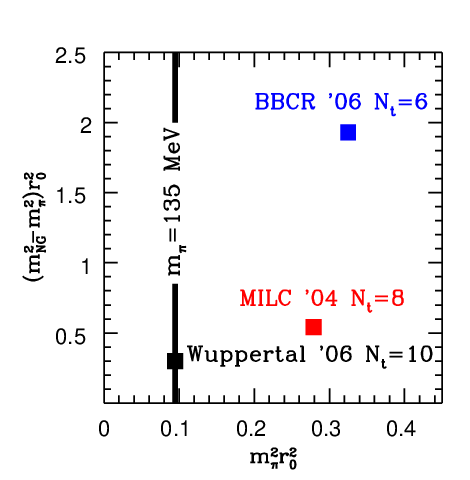
This is the balance one should remember in thermodynamics. Indeed, taste symmetry violation should be suppressed for many reasons (setting the scale at $T=0$, restoring chiral symmetry at $T>0$ etc.) As it was argued above it is more important to improve on this sector of the calculation than on the infinitely high temperature behaviour. The left panel of Figure 2 shows the splitting between the Goldstone and the first non-Goldstone pions for the Bielefeld-Brookhaven- Columbia-Riken Collaboration (which is far beyond their kaon mass), for MILC and for us. Our small splitting is partly related to the stout improvement and partly to the cost issues, since smaller lattice spacings could be used, which resulted in smaller splitting. In addition, the cost issues allowed us to use in our finite T simulations physical quark masses instead of much larger masses.

The next topic to be discussed is the nature of the QCD transition. Physical quark masses were used and a continuum extrapolation was carried out by using four different lattice spacings. The details of the calculations can be found in [8]. In order to determine the nature of the transition one should apply finite size scaling techniques for the chiral susceptibility $\chi=(T/V)\cdot(\partial^{2}\log Z/\partial m_{ud}^{2})$. This quantity shows a pronounced peak as a function of the temperature. For a first order phase transition, such as in the pure gauge theory, the peak of the analogous Polyakov susceptibility gets more and more singular as we increase the volume (V). The width scales with 1/V the height scales with volume (see left panel of Figure 3). A second order transition shows a similar singular behaviour with critical indices. For an analytic transition (what we call a cross-over) the peak width and height saturates to a constant value. That is what we observe in full QCD on $N_{t}$=4 and 6 lattices (middle and right panels of Figure 3). We see an order of magnitude difference between the volumes, but a volume independent scaling. It is a clear indication for a cross-over. These results were obtained with physical quark masses for two sets of lattice spacings. Note, however, that for a final conclusion the important question remains: do we get the same volume independent scaling in the continuum; or we have the unlucky case what we had in the Introduction for 3 flavour QCD (namely the discretization errors changed the nature of the transition for the physical pseudoscalar mass case)?

We carried out a finite size scaling analyses with the continuum extrapolated height of the renormalized susceptibility. The renormalization of the chiral susceptibility can be done by taking the second derivative of the free energy density ($f$) with respect to the renormalized mass ($m_{r}$). We apply the usual definition: $f/T^{4}$ =$-N_{t}^{4}$$\cdot[\log Z(N_{s},N_{t})/(N_{t}N_{s}^{3})-\log Z(N_{s0},N_{t0})/(N_{t0}N_{s0}^{3})]$. This quantity has a correct continuum limit. The subtraction term is obtained at $T$=0, for which simulations are carried out on lattices with $N_{s0}$, $N_{t0}$ spatial and temporal extensions (otherwise at the same parameters of the action). The bare light quark mass ($m_{ud}$) is related to $m_{r}$ by the mass renormalization constant $m_{r}$=$Z_{m}$$\cdot$$m_{ud}$. Note that $Z_{m}$ falls out of the combination $m_{r}^{2}$$\partial^{2}$/$\partial$$m_{r}^{2}$=$m_{ud}^{2}$$\partial^{2}$/$\partial$$m_{ud}^{2}$. Thus, $m_{ud}^{2}\left[\chi(N_{s},N_{t})-\chi(N_{s0},N_{t0})\right]$ also has a continuum limit (for its maximum values for different $N_{t}$, and in the continuum limit we use the shorthand notation $m^{2}$$\Delta\chi$).

In order to carry out the finite volume scaling in the continuum limit we took three different physical volumes (see Figure 4). The inverses of the volumes are shown in units of $T_{c}$. For these 3 physical volumes we calculated the dimensionless combination $T^{4}/m^{2}\Delta\chi$ at 4 different lattice spacings: 0.3 fm was always off, otherwise the continuum extrapolations could be carried out, which are shown on Figure 4. Our result is consistent with an approximately constant behaviour, despite the fact that we had a factor of 5 difference in the volume. The chance probabilities, that statistical fluctuations changed the dominant behaviour of the volume dependence are negligible. As a conclusion we can say that the staggered QCD transition at mu=0 is a cross-over. (Note, that an analytic, cross-over like transition appears in other sector of the standard model, namely for the electroweak transition see e.g. [11] and references therein).

An analytic cross-over, like the QCD transition has no unique $T_{c}$. A particularly nice example for that is the water-vapor transition (c.f. Figure 5). Up to about 650 K the transition is a first order one, which ends at a second order critical point. For a first or second order phase transition the different observables (such as density or heat capacity) have their singularity (a jump or an infinitly high peak) at the same pressure. However, at even higher temperatures the transition is an analytic cross-over, for which the most singular points are different. The blue curve shows the peak of the heat capacity and the red one the inflection point of the density. Clearly, these transition temperatures are different, which is a characteristic feature of an analytic transition (cross-over).

There is another –even more often experienced– example for broad transitions, namely the melting of butter. As we know the melting of ice shows a singular behavior. The transition is of first order, there is only one value of the temperature at which the whole transition takes place at 0^oC (for 1 atm. pressure). Melting of butter¹¹ 1 Natural fats are mixed triglycerids of fatty acids from $C_{4}$ to $C_{24}$, (saturated or unsaturated of even carbon numbers). shows analytic behaviour. The transition is a broad one, it is a cross-over (c.f. Figure 6 for the melting curves of different natural fats).

Since we have an analytic cross-over also in QCD, we expect very similar temperature dependence for the quantities relevant in QCD (e.g. chiral condensate, strange quark susceptibility or Polyakov loop).

In QCD we will study the chiral and the quark number susceptibilities and the Polyakov loop. Usually they give different $T_{c}$ values, but there is nothing wrong with it. As it was illustrated by the water-vapor transition it is a physical ambiguity, related to the analytic behaviour of the transition. There is another, non-physical, ambiguity. If we used different observables (such as the string tension, $r_{0}$, the rho mass or the kaon decay constant), particularly at large lattice spacings we obtain different overall scales. They lead to different $T_{c}$ values. This ambiguity disappeares in the continuum limit. According to our experiences, at finite lattice spacings, the best choice is the kaon decay constant $f_{k}$. It is known experimentally (in contrast to the string tension or $r_{0}$), thus no intermediate calculation with unknown systematics is involved. Furthermore, it can be measured on the lattice quite precisely.

Figure 7 shows the results for the chiral susceptibility, for the quark number susceptibility and for the Polyakov loop. Red, blue, green, and purple indicate $N_{t}$=4,6,8 and 10 lattices. $N_{t}$=4 is always off, the rest scales nicely. The shaded regions indicate the continuum estimates. There is a surprising several sigma effect. The remnant of the chiral transition happens at a quite different temperature than that of the deconfining transition. It is quite a robust statement, since the Polyakov transition region is quite off the $\chi$-peak, and the $\chi$-peak is quite far from the inflection point of the Polyakov loop. This quite large differece is also related to the fact that the transition is fairly broad. The widths are around 30-40 MeV.

Due to the broadness of the transition the normalization prescription changes $T_{c}$, too. It is easy to imagine why, just multiply a Gaussian by $x^{2}$ and the peak is shifted. That means using $\chi/T^{2}$ gives about 10 MeV higher $T_{c}$ than our definition, for which a $T^{4}$ normalization was applied. (Note, that for the unrenormalized $\chi$ a $T^{2}$ normalization is natural, whereas for the renormalized $\chi$ the natural normalization is done by $T^{4}$. This kind of naturalness manifests itself as possibly small errors of the observable.)

Figure 8 shows the difference between the $T_{c}$ values obtained by the Polyakov loop and by the chiral condensate as a function of the lattice spacing squared. The blue band indicates the difference for the chiral susceptibility peak position for the $T^{2}$ and $T^{4}$ normalization. Thus using the $T^{2}$ normalization no difference can be seen for $N_{t}$=4 and 6, a slight difference is observed for $N_{t}$=8 and a reliable continuum extrapolation needs $N_{t}$=6,8 and 10.

Our result on $T_{c}$ and that of the MILC Collaboration ($T_{c}$=169(12)(4) MeV [10]) are consistent within the (quite sizable) errorbars.

However, our result contradicts the recent Bielefeld-Brookhaven-Columbia-Riken result [5], which obtained 192(7)(4) MeV from both the chiral susceptibility and Polyakov loop. This value is about 40 MeV larger than our result for the chiral susceptibility (for the Polyakov loop susceptibility the results agree within about 1.5$\sigma$). What are the differences between their analyses and ours, and how do they contribute to the 40 MeV discrepancy? The most important contributions to the discrepancy are shown by Figure 9. The first difference is, that in [5] no renormalization was carried out, instead they used the unrenormalized quantity $\chi/T^{2}$. Due to the broadness of the distribution this observable leads to about 10 MeV larger $T_{c}$ than our definition. The overall errors can be responsible for another 10 MeV. The origin of the remaining 20 MeV is somewhat more complicated. One possible explanation can be summarized as follows. In Ref. [5] only $N_{t}$=4 and 6 were used, which correspond to lattice spacings a=0.3 and 0.2 fm, or $a^{-1}$=700MeV and 1GeV. These lattices are quite coarse and it seems to be obvious, that no unambiguous scale can be determined for these lattice spacings. The overall scale in Ref. [5] was set by $r_{0}$ and no cross-check was done by any other quantity independent of the static potential (e.g. $f_{k}$). This choice might lead to an ambiguity for the transition temperature, which is illustrated for our data on Figure 10. Using only $N_{t}$=4 and 6 the continuum extrapolated transition temperatures are quite different if one took $r_{0}$ or $f_{K}$ to determine the overall scale. This inconsistency indicates, that these lattice spacing are not yet in the scaling region (similar ambiguity is obtained by using the p4 action of [5]). Having $N_{t}$=4,6,8 and 10 results this ambiguity disappears (as usual $N_{t}$=4 is off), these lattice spacings are already in the scaling region (at least within our accuracy). This phenomenon is not surprising at all. As it was already mentioned e.g. the asqtad action at $N_{t}$$\approx$10 (which corresponds to about a=0.12 fm lattice spacing) has $\approx$10% scale difference predicted by $r_{1}$ or $f_{K}$.

The ambiguity related to the inconsistent continuum limit is unphysical, and it is resolved as we approach the continuum limit (c.f. Figure 10). The differences between the $T_{c}$ values for different observables are physical, it is a consequence of the cross-over nature of the QCD transition.

In the case of the two previous sections (nature of the transition and $T_{c}$) the full results are available in the staggered formalism. This is ensured by the fact that results from three lattice spacings out of four were found to be in the scaling region (c.f. two points are always on a line, thus the real $a^{2}$ behaviour can be read off only by having at least three points). This allowed controlled continuum extrapolations. For the equation of state the situation is not yet satisfactory, our group have results only for two lattice spacings (see also the contribution of F. Karsch [4] for results on the equation of state; they also used two lattice spacings with the p4 action).

Our goal is to determine the temperature dependence of the pressure (or energy density, entropy, speed of sound etc.) of QCD with physical pion mass of 135 MeV along the line of constant physics (LCP). For large homogenous systems the pressure is proportional to the logarithm of the partition function (p$\propto$log[Z]). All other quantities can be determined by using the pressure. Since the partition function itself is difficult to determine the usual technique is to calculate its derivatives and integrate. Thus, for the normalized pressure one obtains

Figure 11 shows the result for the normalized pressure as a function of $T/T_{c}$. The two curves represent $N_{t}$=4 and $N_{t}$=6. Clearly, these two sets of lattice spacings are not enough for a controlled continuum extrapolation. Usually three points in the scaling region is needed to ensure that. Thus, in a fortunate case one could obtain the full result with $N_{t}$=4,6 and 8, whereas a somewhat less fortunate case would mean $N_{t}$=6,8 and 10 (as it was needed for the transition temperature, too). Note, that $N_{t}$=8 needs about 30 times more CPU power than $N_{t}$=6 and $N_{t}$=10 needs an additional factor of about 15.

An old and serious problem for QCD thermodynamics is the link between perturbation theory and lattice QCD. While available lattice results for the equation of state (both for pure gauge theory and for full QCD) end at around $5\cdot T_{c}$, standard perturbation theory converges only at extremely high temperatures (at $5\cdot T_{c}$, the different perturbative orders can not even tell the sign of the deviation from the Stefan-Boltzmann limit). Until recently no link between the two most systematic methods of QCD, namely perturbation theory and lattice QCD, existed for bulk thermodynamical quantities. It is of extreme importance to close the gap between these results (for a recent result on that see [12]).

In the previous three sections results were presented, some of which can be considered as full ones (the nature of the transition and $T_{c}$). For these observables three lattice spacings in the scaling region were used and controlled continuum extrapolations were possible. For another quantity (equation of state) only two lattice spacings were applied, therefore no controlled continuum extrapolated results are available. The situation is even worse for non-vanishing baryonic chemical potentials ($\mu$). In this case traditional Monte-Carlo simulations do not work. The determinant of the Dirac operator turns out to be complex, spoiling any method based on importance sampling. Five years ago new techniques appeared (starting with the multi-parameter reweighting technique [13, 14]), which can give predictions also at $\mu$$\neq$0. Nevertheless, QCD at non-vanishing chemical potentials is much more CPU demanding than the $\mu$=0 case. Thus, continuum extrapolated results will be most probably not available in the next one or two years for most observables. (There is at least one important exception. Using the present methods and technologies one can determine the continuum curvature for the $T$–$\mu$ phase diagram at $\mu$=0.) In this section a few illustrative examples of our $\mu$$\neq$0 results are shown.

According to the most popular scenario a critical point is expected on the temperature versus baryonic chemical potential plane (for an alternative possibility see Ref. [15] and the talk of O. Philipsen in these proceedings [16]). Using the multi-parameter reweighting technique [13, 14] we studied dynamical QCD with $n_{f}$=2+1 staggered quarks of physical masses on $N_{t}$=4 lattices [17]. The results are summarized on Figure 12. At vanishing chemical potentials there is an analytic, cross-over like transition between the hadronic and quark-gluon plasma phases. As we increase $\mu$ the transition temperature decreases. At a baryonic chemical potential around 360 MeV the cross-over region ends and a second order phase transition is observed. For even larger chemical potentials the transition is of first order. In order to tell the difference between an analytic cross-over and a singular transition (first or second order phase transition) a careful finite volume analysis is needed, similar to that of Section 3. This result is quite a different picture than that of Ref. [15]. Note, however that the two results are not at all in contradiction with each other. On the level they can be directly compared both observe no strengthening of the transition in leading order of $\mu$. The strengthening in our result, which is needed for the critical endpoint, appears in much higher orders. (Note, that the same multi-parameter reweighting can be used e.g. to determine the equation of state for non-vanishing baryonic chemical potentials [18, 19].)

Another interesting feature of the $\mu$–$T$ phase diagram is the conjectured colour superconducting phase at large $\mu$ and small $T$. The presently available techniques are working well for small to moderate chemical potentials slightly below and all the way above the transition temperature. In order to extend the applicability range, we used [20] the density of state method. $n_{f}=4$ staggered QCD was studied on $6^{4}$ and $8\cdot 6^{3}$ lattices. The method is expensive, thus only small lattices were used. Nevertheless, these small lattices show an indication for a triple-point connecting three different phases on the phase diagram. The triple point is around $\mu_{q}$$\approx$ 300 MeV and T $\approx$ 135 MeV (the quark chemical potential $\mu_{q}$ is one third of the baryon chemical potential). Note, that the temperature will move most probably to smaller values in the continuum limit, since for $N_{t}$=6 lattices the smallest T is 73 MeV (if $m_{\rho}$ fixes the scale). The mass dependence was checked, at small T the position of the transition did not depend on the pion mass.

It is important to emphasize again that results at non-vanishing chemical potentials are obtained on coarse lattices and the most important uncertainty is the systematic error due to large lattice spacings.

Some QCD thermodynamics results from the Budapest-Wuppertal group were summarized at vanishing and at non-vanishing chemical potentials. The necessary balance between $T=0$ and $T>0$ simulations was discussed in detail. As a consequence, Symanzik improved gauge and stout-link improved staggered fermionic lattice action was used in the simulations with an exact simulation algorithm. Physical masses were taken both for the light quarks and for the strange quark. The parameters were tuned with a quite high precision, thus at all lattice spacings the $m_{K}/f_{k}$ and $m_{K}/m_{\pi}$ ratios were set to their experimental values with an accuracy better than 2%. Up to four sets of lattice spacings on lattices with $N_{t}$=4,6,8 and 10 temporal extensions were used (they correspond to lattice spacing $a$$\sim$0.3, 0.2, 0.15 and 0.12 fm) to carry out the continuum extrapolation. It turned out that only $N_{t}$=6,8 and 10 can be used for a controlled extrapolation, $N_{t}$=4 is out of the scaling region.

The nature of the T$>$0 transition was determined. The renormalized chiral susceptibility was extrapolated to vanishing lattice spacing for three physical volumes, the smallest and largest of which differ by a factor of five. This ensures that a true transition should result in a dramatic increase of the susceptibilities. No such behaviour is observed: the finite-size scaling analysis showed that the finite-temperature QCD transition in the hot early Universe was not a real phase transition, but an analytic crossover (involving a rapid change, as opposed to a jump, as the temperature varied). As such, it will be difficult to find experimental evidence of this transition from astronomical observations. Since for present day heavy ion experiments the baryonic chemical potential is also very small, the above results apply for them, too.

The absolute scale for the T$>$0 transition was calculated. Since the QCD transition is a non-singular cross-over there is no unique $T_{c}$. This well-known phenomenon was illustrated on the water-vapor phase diagram (the broadness of a transition was illustrated by the example of butter). Different observables led to different numerical $T_{c}$ values in the continuum and thermodynamic limit also in QCD. Three observables were used to determine the corresponding transition temperatures. The peak of the renormalized chiral susceptibility predicted $T_{c}$=151(3)(3) MeV, whereas $T_{c}$ based on the strange quark number susceptibility resulted in 24(4) MeV larger value. Another quantity, which is related to the deconfining phase transition in the large quark mass limit is the Polyakov loop. Its behavior predicted a 25(4) MeV larger transition temperature, than that of the chiral susceptibility. Another consequence of the cross-over are the non-vanishing widths of the peaks even in the thermodynamic limit, which were also determined. For the chiral susceptibility, strange quark number susceptibility and Polyakov-loop we obtained widths of 28(5)(1) MeV, 42(4)(1) MeV and 38(5)(1) MeV, respectively.

These features, numbers and functions are attempted to be the full result for the $T$$\neq$0 transition, though other lattice fermion formulations —e.g. Wilson fermions (for ongoing projects see e.g. [21, 22]) or chiral fermions (for an early dynamical overlap test see [23], for the domain wall approach a recent presentation can be found in Ref.[24])— are needed to cross-check the findings with staggered fermions.

Results for the equation of state on lattices with $N_{t}$=4 and 6 were presented. Clearly, one should carry out the calculations on lattices with smaller lattice spacings and approach the continuum limit.

Results at non-vanishing chemical potentials are even further from the continuum limit. At one single lattice spacings we determined the critical endpoint and saw indications for a third phase on the $T$–$\mu$ plane at large baryonic densities. As we emphasized in the abstract of our critical endpoint paper [17] ,,the continuum extrapolation is still missing”. Using the present methods and technologies one can determine the continuum curvature for the $T$–$\mu$ phase diagram at $\mu$=0 in the next few years. Unfortunately, using the present techniques the CPU capacity will be most probably not enough to carry out a controlled continuum extrapolation for the critical endpoint and for a conjectured colour superconducting phase in the next few years.

Partial supports of grants of DFG F0 502/1, EU I3HP, OTKA AT049652 and OTKA K68108 are acknowledged. The author thanks the Budapest-Wuppertal group for collaboration and M. Gyulassy and J.M.K. Szabo for usefull suggestions.