跳到论文正文
W Papers独立论文阅读器 arXiv:0712.2853 论文正文 计算阅读时间 · 0%
引用这篇论文根据当前论文元数据生成,正式投稿前建议核对。


License: Assumed arXiv.org perpetual non-exclusive license
arXiv:0712.2853v1 [math.GT] 18 Dec 2007

On the Lego-Teichmüller game for finite GG-cover

Tanvir Prince
Abstract.

Given a smooth, oriented, closed surface Σ\Sigma of genus zero, possibly with boundary, let Σ~⟶Σ\tilde{\Sigma}\longrightarrow\Sigma be a given GG-cover of Σ\Sigma, where GG is a given finite group. Let SnS_{n} denote the standard sphere with nn holes. There are many ways of gluing together several GG-cover of SnS_{n} to construct the GG-cover Σ~⟶Σ\tilde{\Sigma}\longrightarrow\Sigma, of Σ\Sigma. We let M(Σ~,Σ\tilde{\Sigma},\Sigma) be the set of all ways to construct the given GG-cover, Σ~⟶Σ\tilde{\Sigma}\longrightarrow\Sigma, of Σ\Sigma from gluing of several GG-covers of SnS_{n}, here nn may vary. In this paper, we define some simple moves and relation which will turn M(Σ~,Σ\tilde{\Sigma},\Sigma) into a connected and simply-connected complex. This will be used in the future paper to construct GG-equivariant modular functor. This GG-equivariant modular functor will be an extension of the usual modular functor.

1. Introduction

This paper can be thought of as an extension of the paper “On the Lego-Teichmüller Game” by Bojko Bakalov and Alexander Kirillov Jr [BK]. In the paper [BK], authors gave the description of how to represent a given smooth, oriented surface, possibly with boundary by gluing of several “simple pieces”. Here “simple pieces” are just sphere with nn holes. One application of this is the construction of modular functor; it suffices to define the vector spaces associated with sphere with nn holes. Then since the behavior of modular functor under gluing is known, this defines a unique vector space associated to any surface. Of course, there are many different ways to represent a given surface as a result of gluing several spheres with nn holes, here nn can vary. So some natural questions arise; like how one can describe different ways of gluing “standard pieces” that give the same surface? Let M⁡(Σ)M(\Sigma) be the set of all such way of getting the surface Σ\Sigma from the “simple pieces”. In the paper [BK], they described some simple moves or edges and some relations among them which turned M⁡(Σ)M(\Sigma) into a connected and simply-connected complex.

This definition of modular functor can be extended. Let GG be a finite group. And let Σ~⟶Σ\tilde{\Sigma}\longrightarrow\Sigma be a given GG-cover of Σ\Sigma. It is possible to extend the definition of modular functor from the surface, Σ\Sigma, to the GG-covers of surface, Σ~⟶Σ\tilde{\Sigma}\longrightarrow\Sigma.This idea will be formalized in later paper. This extended modular functor will also satisfy a similar gluing axiom, just like the regular modular functor, but now we are gluing GG-covers of surface and not just surface. Thus if we know the value of the extended modular functor on the “simple pieces”, of course we need to know what are these “simple pieces” in this case, then this will be enough to define Extended modular functor to any GG-cover. Since any GG-cover can be constructed from the gluing of these “simple pieces” and the behavior of the extended modular functor under gluing is known, this will define a unique value for a given GG-cover.

As in the paper of [BK], we are faced with similar questions. Let M⁡(Σ~,Σ)M(\tilde{\Sigma},\Sigma) denote the set of all possible way of gluing together ”simple pieces” to construct the given GG-cover, Σ~⟶Σ\tilde{\Sigma}\longrightarrow\Sigma. Is it possible to define some simple moves to go from one parameterization to the other? Is is possible to define all the relation between these moves? ie describe when a sequence of moves applied to a given parameterization yields the same parameterization? In other word, we are trying to define some simple moves and relations similar to the paper [BK], which will turn M⁡(Σ~,Σ)M(\tilde{\Sigma},\Sigma) into a connected and simply-connected complex. This paper runs side by side with the paper [BK], although there are some differences. It is recommended that readers first read the paper [BK] before reading this one. This paper only deals with the case when the base surface, Σ\Sigma, has genus zero. The case of positive genus will be considered in the subsequent papers.

2. Some basic definition

Let us start with some basic definitions.

2.1. Extended Surface

Definition 1.

An extended surface is a compact, smooth, oriented, closed surface, Σ\Sigma, possibly with boundary and also comes with a choice of distinguished or marked points on each of its boundary component.

We denote by A⁡(Σ)A(\Sigma), the set of the boundary components. So an extended surface will be denoted by (Σ,{pa}a∈A⁡(Σ))(\Sigma,\{p_{a}\}_{a\in A(\Sigma)}) where pap_{a} is the choice of marked point on the aa th boundary component.
Sometimes we will also denote a boundary circle by a Greek letter.

2.2. GG-cover of Extended surface

GG will always denote a finite group, which is given and fixed throughout the whole paper. Let (Σ,{pa}a∈A⁡(Σ))(\Sigma,\{p_{a}\}_{a\in A(\Sigma)}) be an extended surface.

Definition 2.

By a GG cover of (Σ,{pa}a∈A⁡(Σ))(\Sigma,\{p_{a}\}_{a\in A(\Sigma)}), we mean (π:Σ~⟶Σ,{pa~})(\pi:\tilde{\Sigma}\longrightarrow\Sigma,\{\tilde{p_{a}}\}) where (π:Σ~⟶Σ)(\pi:\tilde{\Sigma}\longrightarrow\Sigma) is a principal GG-cover and {pa~}\{\tilde{p_{a}}\} are choice of points on the fiber of pap_{a}. In other word, pa~∈π−1​(pa)​ for all ​a∈A⁡(Σ)\tilde{p_{a}}\in\pi^{-1}(p_{a})\mbox{ for all }a\in A(\Sigma).

2.3. Morphism between GG-cover of extended surface

Definition 3.

Given two GG covers of (Σ,{pa})(\Sigma,\{p_{a}\}) say (π~:Σ~⟶Σ,{pa~})(\tilde{\pi}:\tilde{\Sigma}\longrightarrow\Sigma,\{\tilde{p_{a}}\}) and (π^:Σ^⟶Σ,{pa^})(\hat{\pi}:\hat{\Sigma}\longrightarrow\Sigma,\{\hat{p_{a}}\}), by a morphism between them we mean a homeomorphism f:Σ~→Σ^f:\tilde{\Sigma}\rightarrow\hat{\Sigma} so that the following conditions are satisfied:

i) f⁡(pa~)=pa^f(\tilde{p_{a}})=\hat{p_{a}} for all a∈A⁡(Σ)a\in A(\Sigma)

ii) π^​f=f∗​π~\hat{\pi}f=f_{*}\tilde{\pi}, here f∗:Σ→Σf_{*}:\Sigma\to\Sigma is the homeomorphism we get by restriction of ff to Σ\Sigma

iii) ff preserves the action of GG on each fiber.

See the diagram below:

Σ~\textstyle{\tilde{\Sigma}\ignorespaces\ignorespaces\ignorespaces\ignorespaces\ignorespaces\ignorespaces\ignorespaces\ignorespaces}π~\scriptstyle{\tilde{\pi}}f\scriptstyle{f}Σ^\textstyle{\hat{\Sigma}\ignorespaces\ignorespaces\ignorespaces\ignorespaces}π^\scriptstyle{\hat{\pi}}Σ\textstyle{\Sigma\ignorespaces\ignorespaces\ignorespaces\ignorespaces}f∗\scriptstyle{f_{*}}Σ\textstyle{\Sigma}
Remark 1.

Sometimes, we require f∗:Σ→Σf_{*}:\Sigma\to\Sigma to be the identity.

Although in this definition, we leave the base space fixed, there is no need to do this. We can easily defined morphism between two GG covers where the base space is not fixed.

Definition 4.

Let (π~:Σ~⟶Σ,{pa~})(\tilde{\pi}:\tilde{\Sigma}\longrightarrow\Sigma,\{\tilde{p_{a}}\}) be a GG cover of (Σ,{pa})(\Sigma,\{p_{a}\}) and let (π^:Σ^⟶Σ′,{pa^})(\hat{\pi}:\hat{\Sigma}\longrightarrow{\Sigma^{\prime}},\{\hat{p_{a}}\}) be a GG cover of (Σ′,{pa′})({\Sigma^{\prime}},\{{p_{a}^{\prime}\}}). By a morphism between them, we mean a homeomorphism f:Σ~→Σ^f:\tilde{\Sigma}\rightarrow\hat{\Sigma} so that it satisfies the following condition:
i) f⁡(pa~)=pa^f(\tilde{p_{a}})=\hat{p_{a}} for all pa~\tilde{p_{a}}
ii) ff commutes with the action of GG.

Because of the second condition, it is easily seen that ff descends to a homeomorphism on the base surface by f∗:Σ→Σ′f_{*}:\Sigma\rightarrow{\Sigma^{\prime}} where we defined f∗​(b)=π^​f​(b~)f_{*}(b)=\hat{\pi}f(\tilde{b}) where b~∈π~−1​(b)\tilde{b}\in{\tilde{\pi}}^{-1}(b) . It is easily seen that f∗f_{*} does not depend on the choice of b~\tilde{b}. Also π^​f=f∗​π~\hat{\pi}f=f_{*}\tilde{\pi}.
In other words the diagram below is commutative:

Σ~\textstyle{\tilde{\Sigma}\ignorespaces\ignorespaces\ignorespaces\ignorespaces\ignorespaces\ignorespaces\ignorespaces\ignorespaces}f\scriptstyle{f}π~\scriptstyle{\tilde{\pi}}Σ^\textstyle{\hat{\Sigma}\ignorespaces\ignorespaces\ignorespaces\ignorespaces}π^\scriptstyle{\hat{\pi}}Σ\textstyle{\Sigma\ignorespaces\ignorespaces\ignorespaces\ignorespaces}f∗\scriptstyle{f_{*}}Σ′\textstyle{\Sigma^{\prime}}
Remark 2.

Here we introduce the notation,  MorΣ​(Σ~,Σ~)\mbox{ Mor}_{\Sigma}(\tilde{\Sigma},\tilde{\Sigma}) to denote all the morphisms between the GG-cover Σ~\tilde{\Sigma} and Σ~\tilde{\Sigma} so that the induced map on Σ\Sigma is identity. Also we use the notation  Mor​(Σ~,Σ^)\mbox{ Mor}(\tilde{\Sigma},\hat{\Sigma}) to denote all morphism between GG-cover Σ~\tilde{\Sigma} and Σ^\hat{\Sigma} where the induced map on the base surface can be anything.

2.4. Orientation of the boundary circle

The orientation of the extended surface, Σ\Sigma, naturally induces orientation on the boundary circle. We want to explain this in a little detail. Let D={z∈ℂ||z|<1}D=\{z\in\mathbb{C}||z|<1\}. First, we fix an orientation on the complement of DD. This orientation is given by the choice of the basis, {1,i}\{1,i\},on ℂ\mathbb{C}, and the counterclockwise orientation on the unit circle. See the figure 1.

Refer to caption
Figure 1. orientation on the complement of the unit disk

Now for each boundary circle of Σ\Sigma, we choose a small neighborhood around the circle. This neighborhood is homeomorphic to E={z∈ℂ|1≤|z|≤1+ϵ}E=\{z\in\mathbb{C}|1\leq|z|\leq 1+\epsilon\} for some ϵ\epsilon. For any such homeomorphism which preserve the orientation of the surface, there is an unique choice of orientation of the boundary circle of Σ\Sigma so that the map also preserve the orientation on the boundary. This gives an orientation to each boundary component of Σ\Sigma.

2.5. Monodromy

2.5.1. Definition of Monodromy

Monodromy will be an important tool to describe GG-cover. In fact soon we will prove that two GG-covers of a surface of genus 0 are isomorphic iff their monodromy is same.

Definition 5.
:

[Monodromy around a boundary circle:] Let (π:Σ~⟶Σ,{pa~})(\pi:\tilde{\Sigma}\longrightarrow\Sigma,\{\tilde{p_{a}}\}) be a GG-cover of (Σ,{pa}a∈A⁡(Σ))(\Sigma,\{p_{a}\}_{a\in A(\Sigma)}). Consider the aa th boundary circle, SS, where the base point on SS is pap_{a} and the point on the fiber above is pa~\tilde{p_{a}}. This SS has an orientation which comes from the orientation of the surface. Let α:[0,1]→S\alpha:[0,1]\rightarrow S be a parameterization of the boundary circle SS which also preserves the orientation of SS. We also assume that α⁡(0)=α⁡(1)=pa\alpha(0)=\alpha(1)=p_{a}. Then there is a unique lifting of α\alpha to the GG-cover, say α~:[0,1]→Σ~\tilde{\alpha}:[0,1]\rightarrow\tilde{\Sigma} such that α~​(0)=pa~\tilde{\alpha}(0)=\tilde{p_{a}}. We define the monodromy, m∈Gm\in G, of this aa th boundary circle to be that unique element of GG such that

(1) m​α~​(0)=α~​(1)m\tilde{\alpha}(0)=\tilde{\alpha}(1)
Lemma 1.

Monodromy does not depend on the choice of parameterization

Proof.

This is not hard to see. From the definition, we see that the monodromy only depends on the starting point of the lifting; if we know the starting point of the lifting, everything else is determined by the cover, including the end point of the lifting. And monodromy only depends on the starting point and the ending point of the lifting. The details are left for the reader. ∎

2.5.2. Relation Between Monodromy and Lifting of a Map

Given two GG-covers and a map between their base surfaces, we want to know under what condition this map can be lifted to the covers. Monodromy helps us to partially answer this question. We have the following lemma.

Lemma 2.

Let (π~:Σ~⟶Σ,{pa~})(\tilde{\pi}:\tilde{\Sigma}\longrightarrow\Sigma,\{\tilde{p_{a}}\}) be a GG cover of (Σ,{pa})(\Sigma,\{p_{a}\}) and let (π^:Σ^⟶Σ′,{pa^})(\hat{\pi}:\hat{\Sigma}\longrightarrow{\Sigma^{\prime}},\{\hat{p_{a}}\}) be a GG cover of (Σ′,{pa′})({\Sigma^{\prime}},\{{p_{a}^{\prime}}\}). Here we also assume the base surfaces to be connected. Let f:Σ→Σ′f:\Sigma\rightarrow{\Sigma^{\prime}} be a homeomorphism of the base surfaces which maps marked points to marked points, that is f⁡(pa)=pa′f(p_{a})={p_{a}^{\prime}}. See the diagram below:

Σ~\textstyle{\tilde{\Sigma}\ignorespaces\ignorespaces\ignorespaces\ignorespaces\ignorespaces\ignorespaces\ignorespaces\ignorespaces}f~\scriptstyle{\tilde{f}}π~\scriptstyle{\tilde{\pi}}Σ^\textstyle{\hat{\Sigma}\ignorespaces\ignorespaces\ignorespaces\ignorespaces}π^\scriptstyle{\hat{\pi}}Σ\textstyle{\Sigma\ignorespaces\ignorespaces\ignorespaces\ignorespaces}f\scriptstyle{f}Σ′\textstyle{\Sigma^{\prime}}

Then

  1. (1)

    The lifting of ff to GG-covers Σ~⟶Σ^\tilde{\Sigma}\longrightarrow\hat{\Sigma} is unique, if it exists at all.

  2. (2)

    If in addition, we assume that the genus of both base surfaces are 0, then ff can be lifted iff monodromy of the two GG-covers match. That is

    m⁡((∂Σ)i)=m⁡(f​(∂Σ)i)m((\partial\Sigma)_{i})=m(f(\partial\Sigma)_{i})

    where m⁡((∂Σ)i)m((\partial\Sigma)_{i}) = monodromy of (∂Σ)i(\partial\Sigma)_{i} boundary circle of Σ\Sigma.
    and m⁡(f​(∂Σ)i)m(f(\partial\Sigma)_{i}) = monodromy of f​(∂Σ)if(\partial\Sigma)_{i} boundary circle of Σ′\Sigma^{\prime}.
    Note that the homeomorphism, f:Σ→Σ′f:\Sigma\rightarrow{\Sigma^{\prime}}, maps the boundary components of Σ\Sigma to the boundary components of Σ′\Sigma^{\prime}.

Proof.

(1) is obvious. To be more specific, let f1f_{1} and f2f_{2} be two lifting of ff. From the definition of lifting and morphism of GG covers (see 2.3), f1f_{1} and f2f_{2} must satisfy

π^​f1=π^​f2=f​π~\hat{\pi}f_{1}=\hat{\pi}f_{2}=f\tilde{\pi}

So if x∈Σx\in\Sigma then both f1f_{1} and f2f_{2} maps the fiber above the xx to the fiber above the f⁡(x)f(x). Moreover from the definition of morphism between GG-cover we must have f1​(pa~)=f2​(pa~)=pa^f_{1}(\tilde{p_{a}})=f_{2}(\tilde{p_{a}})=\hat{p_{a}}
Also both f1f_{1} and f2f_{2} commute with the action of GG. This information guarantees that they must agree on all the fibers of same connected component. But since our base surfaces are connected they must agree everywhere. So f1f_{1} = f2f_{2}.

For (2), we will use the following standard proposition of GG cover:

Proposition 1.

Let π~:Σ~→Σ\tilde{\pi}:\tilde{\Sigma}\to\Sigma and π^:Σ^→Σ′\hat{\pi}:\hat{\Sigma}\to\Sigma^{\prime} be two GG covers and f:Σ→Σ′f:\Sigma\to\Sigma^{\prime} be a map between the base surface. Then this map, ff can be lifted to the GG cover if and only if the monodromy of every loop, α\alpha, in π~:Σ~→Σ\tilde{\pi}:\tilde{\Sigma}\to\Sigma is equal to the monodromy of the corresponding loop, f⁡(α)f(\alpha), in π^:Σ^→Σ′\hat{\pi}:\hat{\Sigma}\to\Sigma^{\prime}. And in the case that both of the base surfaces, Σ\Sigma and Σ′\Sigma^{\prime}, have genus zero, then ff can be lifted to the GG covers if and only if the monodromy of the corresponding boundary circles match.

Proof.

A proof of this or some equivalent statements can be found in many standard books on topology. For example see section 1.3 of [AH]. ∎

From the above proposition, the statement 2 of our lemma easily followed.

∎

2.6. Gluing of two GG-covers of extended surfaces

Definition 6.

Let (π~:Σ~⟶Σ,{pa~})(\tilde{\pi}:\tilde{\Sigma}\longrightarrow\Sigma,\{\tilde{p_{a}}\}) be a GG cover of (Σ,{pa})(\Sigma,\{p_{a}\}) and let (π^:Σ^⟶Σ′,{pa^})(\hat{\pi}:\hat{\Sigma}\longrightarrow{\Sigma^{\prime}},\{\hat{p_{a}}\}) be a GG cover of (Σ′,{pa′})({\Sigma^{\prime}},\{{p_{a}^{\prime}\}}). Let si,j:(∂Σ)i→(∂Σ′)js_{i,j}:(\partial\Sigma)_{i}\to(\partial\Sigma^{\prime})_{j} be an orientation reversing map of the iith boundary circle of Σ\Sigma to the jj th boundary circle of Σ′\Sigma^{\prime} so that si,j​(pi)=pj′s_{i,j}(p_{i})=p_{j}^{\prime}. Then we define the gluing of these two GG covers under si,js_{i,j} to be the following GG cover:

π~​⨆si,jπ^:Σ~​⨆si,jΣ^⟶Σ​⨆si,jΣ′\tilde{\pi}\bigsqcup_{s_{i,j}}\hat{\pi}:\tilde{\Sigma}\bigsqcup_{s_{i,j}}\hat{\Sigma}\longrightarrow\Sigma\bigsqcup_{s_{i,j}}\Sigma^{\prime}

where Σ​⨆si,jΣ′\Sigma\bigsqcup_{s_{i,j}}\Sigma^{\prime} is the surface obtained by identifying points on (∂Σ)i(\partial\Sigma)_{i} to the points on (∂Σ′)j(\partial\Sigma^{\prime})_{j} through the map si,js_{i,j}. And Σ~​⨆si,jΣ^\tilde{\Sigma}\bigsqcup_{s_{i,j}}\hat{\Sigma} is the GG cover obtained by identifing a point (t,g)(t,g), where t∈(∂Σ)it\in(\partial\Sigma)_{i} and g∈Gg\in G, to the point (si,j​(t),g)(s_{i,j}(t),g).

2.6.1. How to glue two GG-covers

Such a gluing not always exists, but if it exists, it is unique. So we have the following lemma.

Lemma 3.

Let (π~:Σ~⟶Σ,{pa~})(\tilde{\pi}:\tilde{\Sigma}\longrightarrow\Sigma,\{\tilde{p_{a}}\}) be a GG cover of (Σ,{pa})(\Sigma,\{p_{a}\}) and let (π^:Σ^⟶Σ′,{pa^})(\hat{\pi}:\hat{\Sigma}\longrightarrow{\Sigma^{\prime}},\{\hat{p_{a}}\}) be a GG cover of (Σ′,{pa′})({\Sigma^{\prime}},\{{p_{a}^{\prime}\}}). Take b∈A⁡(Σ)b\in A(\Sigma) and c∈A⁡(Σ′)c\in A(\Sigma^{\prime}). We want to glue (∂Σ)b{(\partial{\Sigma})}_{b} and (∂Σ′)c{(\partial{{\Sigma^{\prime}}})}_{c}. Then :

  1. (1)

    If the gluing exists, there is a unique way, up to isomorphism of GG covers, to glue these GG-covers

  2. (2)

    Gluing is possible iff the monodromy, mbm_{b}, of (∂Σ)b({\partial\Sigma})_{b} and the monodromy, mcm_{c} of (∂Σ′)c({\partial\Sigma}^{\prime})_{c} are inverse of each other. That is mb​mc=1m_{b}m_{c}=1.

Proof.

Not only we need to glue (∂Σ)b({\partial\Sigma})_{b} and (∂Σ′)c({\partial\Sigma}^{\prime})_{c} but we also need to glue the cover above it. See the diagram on figure 2.

Refer to caption
Figure 2. Fiber of the two boundary circles we want to glue

We identify pb∈(∂Σ)bp_{b}\in({\partial\Sigma})_{b} with pc′∈(∂Σ′)c{p_{c}^{\prime}}\in{({\partial\Sigma}^{\prime})}_{c} and this will basically tells us how to glue (∂Σ)b{({\partial\Sigma})}_{b} with (∂Σ′)c({\partial\Sigma}^{\prime})_{c} since, first of all the orientation of the boundary circle comes from the orientation of the surface, and the set of all orientation preserving homeomorphisms from (∂Σ)b{({\partial\Sigma})}_{b} to (∂Σ′)c({\partial\Sigma}^{\prime})_{c} which map pbp_{b} to pc′{p_{c}^{\prime}} is homotopic to each other. This is how we glue (∂Σ)b{({\partial\Sigma})}_{b} with (∂Σ′)c{({\partial\Sigma}^{\prime})}_{c} . Now what about the cover? Let us take a small neighborhood of pbp_{b} and pc′{p_{c}^{\prime}} on the circle (∂Σ)b{({\partial\Sigma})}_{b} and (∂Σ′)c{({\partial\Sigma}^{\prime})}_{c} so that the fiber above these neighborhoods of circles break up into disjoint pieces and each piece maps homeomorphically by π~\tilde{\pi} and π^\hat{\pi} to these neighborhoods of circle. see the diagram on figure 3

Refer to caption
Figure 3. Neighborhood of distinguished points and the fiber above it

One of the pieces on the left contains pb~\tilde{p_{b}} and one of the piece on the right contains pc^\hat{p_{c}}. Also GG acts simply transitively on these pieces. By definition, we require the piece containing pb~\tilde{p_{b}} to be glued with the piece containing pc^\hat{p_{c}} so that the action of GG commutes with the gluing. This fixes how the pieces of GG-cover containing pb~\tilde{p_{b}} will be glued to the pieces of GG-cover containing pc^\hat{p_{c}}. Now we move around the circle and repeat the same process until we cover the whole circle, (∂Σ)b({\partial\Sigma})_{b} and (∂Σ′)c({\partial\Sigma}^{\prime})_{c}.

This tells us that there is at most one way to glue. Note that not always we can glue two GG- covers. For example take |G|=2|G|=2. Take one GG-cover to be the trivial GG-cover of the circle and the other GG-cover to be the double cover of the circle. These two GG-covers can not be glued.

The second part of the lemma is left to the reader. Basically one sees that as we moved around the whole circle and then glue or we first glue and then move around the whole circle, in either case we arrived at the same point since the monodromy are inverse of each other. So we don’t have any problem to glue. Readers can supply the detail. ∎

3. Standard block

3.1. Standard sphere, SnS_{n}

For every n≥0n\geq 0, we define the standard sphere, SnS_{n}, to be the Reimann sphere ℂ¯\overline{\mathbb{C}} with nn disks |z−k|<13|z-k|<\frac{1}{3} removed and with the marked points being k−i3k-\frac{i}{3}, here k=1,2,3,…​nk=1,2,3,...n. Of course, we could replace these nn disks with any other nn non-overlapping disks with centers on the real line and with marked points in the lower half plane. Any two such spheres are homeomorphic and the homeomorphism can be chosen canonically up to homotopy. Note that the set of boundary components of the standard sphere is naturally indexed by numbers 1,2,…​n1,2,...n. The standard sphere, S4S_{4}, with four holes is shown on figure 4

Refer to caption
Figure 4. A standard sphere with four holes where the marked points are denoted by p1,…​p4p_{1},...p_{4}

3.2. Standard blocks, Sn​(g1,…,gn,h1,…,hn)S_{n}(g_{1},...,g_{n};h_{1},...,h_{n})

In the paper [BK], where |G|=1|G|=1, standard blocks are just these standard spheres,Sn,n=1.2​…S_{n},n=1.2.... So we need to extend this definition to the general case where GG is a finite group. To do this we start with the following construction. Let us start with a standard sphere with nn holes, SnS_{n} and 2​n2n elements from GG where we denote these 2​n2n elements as {g1,…,gn}\{g_{1},...,g_{n}\} and {h1,…,hn}\{h_{1},...,h_{n}\} and we also required that g1​…​gn=1g_{1}...g_{n}=1. First we make the cuts on SnS_{n} as in figure 5.

Refer to caption
Figure 5. Cuts on SnS_{n}

Here the point q∈Snq\in S_{n} in figure 5 is the point at ∞\infty. In fact qq can be chosen to be any point on the upper hemisphere as long as it does not belong to the boundary circles. Then one can easily sees that Sn\S_{n}\backslashcuts is simply connected. So GG-cover of Sn\S_{n}\backslashcuts is trivial. In other word, GG-cover of Sn\S_{n}\backslashcuts looks like

Sn\ cuts ×G\textstyle{S_{n}\backslash\mbox{ cuts }\times G\ignorespaces\ignorespaces\ignorespaces\ignorespaces}Sn\ cuts \textstyle{S_{n}\backslash\mbox{ cuts }}

Although there is only one GG cover of Sn\S_{n}\backslashcuts up to isomorphism, there are a total of |G||G| many way to identify GG cover of Sn\S_{n}\backslashcuts with GG, but the important thing here to notice is that any such identification is isomorphic. So we chose one such identification. Now consider the iith cut. We want to glue the fiber on the left hand side of the iith cut with the fiber on the right hand side of the iith cut. This identification must preserve the action of the group GG. Thus the identification can be given by a multiplication on the right by some element of the group GG. We chose this element to be gi∈Gg_{i}\in G. That is we glued along the iith cut by multiplication of the right by gig_{i}. See figure 6.

Refer to caption
Figure 6. A point xx on the left hand side of the fiber of the iith cut is glued to x​gixg_{i} on the right hand side

Now we choose pi~=(pi,hi)\tilde{p_{i}}=(p_{i},h_{i}) as the choice of point in the fiber of pip_{i}. Thus we end up with a GG cover of SnS_{n}. The reason we require that g1​…​gn=1g_{1}...g_{n}=1 is easy to see. Consider a point (t,x), where ​x∈G(t,x),\mbox{ where }x\in G, on the GG-cover. As we moved along each cut, we multiply on the right by gig_{i}. After moving along all the cut, we end up with ( some point on of the base surface ,x​g1​g2​…​gn)(\mbox{ some point on of the base surface },xg_{1}g_{2}...g_{n}), but then we must have x=x​g1​g2​…​gnx=xg_{1}g_{2}...g_{n} or equivalently g1​…​gn=1g_{1}...g_{n}=1. Thus from the data g1,…,gng_{1},...,g_{n} and h1,…,hnh_{1},...,h_{n} where g1​…​gn=1g_{1}...g_{n}=1, we have constructed a GG cover of SnS_{n}.

Definition 7.

The GG cover of SnS_{n} constructed above is called standard block and will be denoted by Sn(g1,g2….,gn;h1,h2….,hn)S_{n}(g_{1},g_{2}....,g_{n};h_{1},h_{2}....,h_{n}) where we always assume that g1​g2​…​gn=1g_{1}g_{2}...g_{n}=1 although we do not always write this explicitly.

3.3. When two standard blocks are isomorphic

Given two GG-covers of SnS_{n}, we want to know when they are isomorphic, hence the following lemma:

Lemma 4.

Let Sn(g1,….gn;h1,…hn)S_{n}(g_{1},....g_{n};h_{1},...h_{n}) and Sn(g1′,….gn′;h1′…hn′)S_{n}(g_{1}^{\prime},....g_{n}^{\prime};h_{1}^{\prime}...h_{n}^{\prime}) be two standard blocks. Then they are isomorphic iff ∃x∈G\exists x\in G so that x​gi​x−1=gi′xg_{i}x^{-1}=g_{i}^{\prime} and hi​x−1=hi′h_{i}x^{-1}=h_{i}^{\prime} for i=1​…​ni=1...n. We denote the isomorphism, Sn​(𝐠,𝐡)→Sn​(𝐠′,𝐡′)S_{n}(\mathbf{g,h})\to S_{n}(\mathbf{g^{\prime},h^{\prime}}) by ϕx\phi_{x}.

Proof.

First assume Sn(g1,….gn;h1,…hn)S_{n}(g_{1},....g_{n};h_{1},...h_{n}) and Sn(g1′,….gn′;h1′…hn′)S_{n}(g_{1}^{\prime},....g_{n}^{\prime};h_{1}^{\prime}...h_{n}^{\prime}) are isomorphic. This means there exist an isomorphism of GG-cover which by definition (see section 2.3 on page 2.3) maps (pi,hi)⟶(pi,hi′)(p_{i},h_{i})\longrightarrow(p_{i},h_{i}^{\prime}) and preserve the GG-action. So on the fiber, this isomorphism is just the right multiplication by some element x−1∈Gx^{-1}\in G. Also the following condition must satisfy along the cut:
First glue and then apply isomorphism == First apply isomorphism and then glue.
In other word, if tt is a point on the fiber above the iith cut, then we must have

t​gi​x−1=t​x−1​gi′\displaystyle tg_{i}x^{-1}=tx^{-1}g_{i}^{\prime}
or ​gi′=x​gi​x−1​ for ​i=1​…​n\displaystyle\mbox{ or }g_{i}^{\prime}=xg_{i}x^{-1}\mbox{ for }i=1...n

And of course we must have hi​x−1=hi′h_{i}x^{-1}=h^{\prime}_{i} from the definition of isomorphism of two GG-cover.
The other direction is easier to show. We define the isomorphism on each fiber through the multiplication on the right by x−1x^{-1}. This can be easily seen to satisfy all the required property of isomorphism. ∎

3.4. Monodromy of a Standard Block

The next natural question is to ask what is the monodromy of the standard block, Sn​(g1,g2​…​gn,h1,h2​…​hn)S_{n}(g_{1},g_{2}...g_{n};h_{1},h_{2}...h_{n}). So we have the following lemma:

Lemma 5.

Let Sn(g1,….gn;h1,…hn)S_{n}(g_{1},....g_{n};h_{1},...h_{n}) be a GG-cover of SnS_{n}. Here we assume the orientation of the boundary circles induces by the outward normal vector according to the right hand rule. See section 2.4 on page 2.4 for the discussion of how the orientation of the surface induces orientation on the boundary. See the picture on figure 7.

Refer to caption
Figure 7. observe the orientation of the boundary circles

Then the monodromy mi∈Gm_{i}\in G around the iith boundary circle is given by:

mi=hi​gi−1​hi−1m_{i}=h_{i}g_{i}^{-1}h_{i}^{-1}
Proof.

Given a parameterization α\alpha : [0,1] ⟶\longrightarrow iith boundary circle of SnS_{n}, we lift this path starting from (pi,hi)(p_{i},h_{i}), and as we cross the cut labeled by gig_{i} from right to left, we end up with (∗,hi​gi−1)(*,h_{i}g_{i}^{-1}). See the picture on figure 8.

Refer to caption
Figure 8.

And as we continue all the way, at the end we arrive at the point (pi,hi​gi−1)(p_{i},h_{i}g_{i}^{-1}). So from the definition of monodromy, the iith monodromy mi∈Gm_{i}\in G is given by

mi​hi=hi​gi−1​ so\displaystyle m_{i}h_{i}=h_{i}g_{i}^{-1}\mbox{ so }
mi=hi​gi−1​hi−1\displaystyle m_{i}=h_{i}g_{i}^{-1}h_{i}^{-1}

∎

3.5. Gluing of two standard blocks

Let the standard block Sn​(g1,…,gn,h1,…,hn)S_{n}(g_{1},...,g_{n};h_{1},...,h_{n}) and Sm​(u1,…,um,v1,…,vm)S_{m}(u_{1},...,u_{m};v_{1},...,v_{m}) are given. We want to know when we can glue these two standard blocks along the ii th boundary circle of Sn​(g1,…,gn,h1,…,hn)S_{n}(g_{1},...,g_{n};h_{1},...,h_{n}) to the jj th boundary circle of Sm​(u1,…,um,v1,…,vm)S_{m}(u_{1},...,u_{m};v_{1},...,v_{m}). Hence we have the following lemma:

Lemma 6.

ii th boundary circle of Sn​(g1,…,gn,h1,…,hn)S_{n}(g_{1},...,g_{n};h_{1},...,h_{n}) can be glued to the jj th boundary circle of Sm​(u1,…,um,v1,…,vm)S_{m}(u_{1},...,u_{m};v_{1},...,v_{m}) iff hi​gi−1​hi−1=[vj​uj−1​vj−1]−1h_{i}g_{i}^{-1}h_{i}^{-1}=[v_{j}u_{j}^{-1}v_{j}^{-1}]^{-1}.

Proof.

According to lemma 5 on page 5, monodromy of the ii th boundary circle of Sn​(g1,…,gn,h1,…,hn)S_{n}(g_{1},...,g_{n};h_{1},...,h_{n}) is given by hi​gi−1​hi−1h_{i}g_{i}^{-1}h_{i}^{-1} and the monodromy of the jj th boundary circle of Sm​(u1,…,um,v1,…,vm)S_{m}(u_{1},...,u_{m};v_{1},...,v_{m}) is given by vj​uj−1​vj−1v_{j}u_{j}^{-1}v_{j}^{-1}. Now according to the lemma 3 on page 3, such a gluing exist if and only if these two monodromy are inverse of each other, that is hi​gi−1​hi−1=[vj​uj−1​vj−1]−1h_{i}g_{i}^{-1}h_{i}^{-1}=[v_{j}u_{j}^{-1}v_{j}^{-1}]^{-1}. ∎

Remark 3.

We will use the notation

Sn​(g1,…,gn,h1,…,hn)​⨆c,hi,vjSm​(u1,…,um,v1,…,vm)S_{n}(g_{1},...,g_{n};h_{1},...,h_{n})\bigsqcup_{c,h_{i},v_{j}}S_{m}(u_{1},...,u_{m};v_{1},...,v_{m})

to indicate that the iith boundary of the left standard block is glued along the cut cc to the jjth boundary of the right standard block.

3.6. Groupoid

Definition 8.

A category is called a groupoid if all of its morphism is invertible.

We list two important examples of groupoid which will be needed later.

Example 1.

For a fixed SnS_{n}, consider the category, YnY_{n}, defined in the following way:
obj(YnY_{n})= GG-covers of SnS_{n}
mor(YnY_{n})= isomorphisms of GG-covers which are trivial on SnS_{n}.
Since only morphisms are isomorphisms, this is obviously a groupoid.

Example 2.

We define the category TnT_{n} in the following way:
obj(TnT_{n}) =
{standard blocks} = {Sn(g1,g2,….gn;h1,h2…hn)|gi∈G and hi∈G for i=1…n and g1g2…gn=1}\{S_{n}(g_{1},g_{2},....g_{n};h_{1},h_{2}...h_{n})|g_{i}\in G\mbox{ and }h_{i}\in G\mbox{ for }i=1...n\mbox{ and }g_{1}g_{2}...g_{n}=1\}
According to lemma in 3.3 on page 3.3 all the isomorphism between two standard block can be defined in the following way:
mor(Sn(g1,g2,….gn;h1,h2…hn),Sn(g1′,g2′,….gn′;h1′,h2′…hn′)S_{n}(g_{1},g_{2},....g_{n};h_{1},h_{2}...h_{n}),S_{n}(g_{1}^{{}^{\prime}},g_{2}^{{}^{\prime}},....g_{n}^{{}^{\prime}};h_{1}^{{}^{\prime}},h_{2}^{{}^{\prime}}...h_{n}^{{}^{\prime}}))={x∈G|xgix−1=gi′ and hix−1=hi′ for i=1…n}\{x\in G|xg_{i}x^{-1}=g_{i}^{{}^{\prime}}\mbox{ and }h_{i}x^{-1}=h_{i}^{{}^{\prime}}\mbox{ for }i=1...n\}. Since given a morphism x∈Gx\in G in this category the inverse morphism is x−1∈Gx^{-1}\in G, every morphism is invertible. So the category TnT_{n} is in fact a groupoid.

We have the following important lemma:

Lemma 7.

The groupoid YnY_{n} is equivalent to the groupoid TnT_{n}. See example 1 and 2 above for the description of YnY_{n} and TnT_{n}.

Proof.

To prove this lemma, we will use a well known theorem from category theory.

Theorem 1.

Let AA and BB be two categories, and F:A→BF:A\rightarrow B is a covariant functor, so that the following two conditions hold:

  1. (1)

    For any two objects, X,Y∈ Obj ​(A)X,Y\in\mbox{ Obj }(A), the map  Mor A​(X,Y)⟶ Mor B​(F⁡(X),F⁡(Y))\mbox{ Mor }_{A}(X,Y)\longrightarrow\mbox{ Mor }_{B}(F(X),F(Y)), induced by FF, is bijective.

  2. (2)

    The map FF is essentially surjective. That is given any object, V∈ Obj ​(B)V\in\mbox{ Obj }(B), there exist an object, U∈ Obj (A)U\in\mbox{ Obj }(A) so that F⁡(U)≅VF(U)\cong V. Here the symbol ≅\cong means isomorphic.

Then FF is in fact an equivalence of categories.

Proof.

For a proof of this theorem, see any standard book on category theory, for example “Categories for the working Mathematician” by Mac Lane, see [C]. ∎

Now let us come back to the proof of our lemma. We will construct a functor V:Tn→YnV:T_{n}\rightarrow Y_{n} so that VV satisfies the two conditions of Theorem 1. Then this VV will define the equivalence between TnT_{n} and YnY_{n}. Given a standard block, Sn(g1,g2,….gn;h1,h2…hn) where gi∈G and hi∈G for i=1…n and g1g2…gn=1S_{n}(g_{1},g_{2},....g_{n};h_{1},h_{2}...h_{n})\mbox{ where }g_{i}\in G\mbox{ and }h_{i}\in G\mbox{ for }i=1...n\mbox{ and }g_{1}g_{2}...g_{n}=1, this standard block, in particular, a GG cover of SnS_{n}. That is

V(Sn(g1,g2,….gn;h1,h2…hn))= the G cover of Sn corresponding to the standard block V(S_{n}(g_{1},g_{2},....g_{n};h_{1},h_{2}...h_{n}))=\mbox{ the $G$ cover of $S_{n}$ corresponding to the standard block }

Similarly, if ϕx:Sn(g1,g2,….gn;h1,h2…hn)→Sn(g1′,g2′,….gn′;h1′,h2′…hn′)\phi_{x}:S_{n}(g_{1},g_{2},....g_{n};h_{1},h_{2}...h_{n})\rightarrow S_{n}(g^{\prime}_{1},g^{\prime}_{2},....g^{\prime}_{n};h^{\prime}_{1},h^{\prime}_{2}...h^{\prime}_{n}) is a morphism between two standard blocks, then V⁡(ϕx)V(\phi_{x}) is the same morphism between the GG covers.

To show, this functor VV satisfies the condition 11 of the above theorem, we just refer to the lemma 4 on page 4. First note that, by this lemma, given any two standard blocks, either there exist an unique morphism, ϕx\phi_{x}, between them or there is no morphism between them. In either case, the condition 11 is obviously satisfied.

For condition 2, let π:Sn~→Sn\pi:\tilde{S_{n}}\rightarrow S_{n} be a GG-cover of SnS_{n}. First, we make the same cuts on SnS_{n} as figure 5 on page 5. Then the GG-cover of Sn\S_{n}\backslashcuts is trivial. In other word, the GG-cover of Sn\S_{n}\backslashcuts can be identified with

Sn\ cuts ×G\textstyle{S_{n}\backslash\mbox{ cuts }\times G\ignorespaces\ignorespaces\ignorespaces\ignorespaces}Sn\ cuts \textstyle{S_{n}\backslash\mbox{ cuts }}

Now we need to identify the components of Sn\ cuts ×GS_{n}\backslash\mbox{ cuts }\times G with the group GG. Here we have choice. So we make some choice, it does not matter how we want to do this. Now we basically repeat the same construction when we describe standard blocks, namely, from this trivial cover, to get the original cover we started with, we need to glue the cover along the cuts. See the picture on figure 9.

Refer to caption
Figure 9.

This gluing must preserve the action of GG on the fiber. So to glue along the ii-th cut, there must exist gi∈Gg_{i}\in G so that the point tt on one side of the cut must glued with the point t​gitg_{i} from the other side of the cut. Thus for a total of n-cut we get {g1,g2​…​gn∈G}\{g_{1},g_{2}...g_{n}\in G\}. Also to start with, our GG-cover comes with a point (pi,hi)(p_{i},h_{i}) on the fiber above pip_{i}. This gives us {h1,h2​…​hn∈G}\{h_{1},h_{2}...h_{n}\in G\}. To show g1​…​gn=1g_{1}...g_{n}=1 is easy. Consider a point (t,x), where ​x∈G(t,x),\mbox{ where }x\in G, on the GG-cover. As we moved along each cut, we multiply on the right by gig_{i}. After moving along all the cut, we end up with ( some point on of the base surface ,x​g1​g2​…​gn)(\mbox{ some point on of the base surface },xg_{1}g_{2}...g_{n}), but then we must have x=x​g1​g2​…​gnx=xg_{1}g_{2}...g_{n} or equivalently g1​…​gn=1g_{1}...g_{n}=1. Thus the GG cover Sn~\tilde{S_{n}} is isomorphic to the standard block Sn​(g1,…​gn,h1,…​hn)S_{n}(g_{1},...g_{n};h_{1},...h_{n}). This shows that the functor VV satisfies the second requirement of the above theorem. ∎

Remark 4.

In particular, the above theorem shows that every GG cover of SnS_{n} is isomorphic to a standard block.

3.7. Review of the parameterization for the case |G|=1|G|=1

For the readers convenience, we will review the concept of parameterization for the trivial case, |G|=1|G|=1, from [BK]. We begin with some definitions.

Definition 9.

Let Σ\Sigma be an extended surface. A cut system, CC, on Σ\Sigma is a finite collection of smooth, simple closed non-intersecting curves on Σ\Sigma such that each connected component of the complement, Σ\C\Sigma\backslash C, is a surface of genus zero. In this paper, we will always assume the surface Σ\Sigma has genus 00. So in this case, the requirement that each connected component of the complement, Σ\C\Sigma\backslash C, is a surface of genus zero is always satisfied.

An example of a cut system is given in figure 10.

Refer to caption
Figure 10. An example of a cut system
Definition 10.

Let Σ\Sigma be an extended surface with genus zero. A parameterization without cuts of Σ\Sigma is a homotopy equivalence class of homeomorphisms ϕ:Σ≃Sn\phi:\Sigma\simeq S_{n}, where SnS_{n} is the standard sphere with nn holes.

Definition 11.

Let Σ\Sigma be a an extended surface. A parameterization, PP, of Σ\Sigma is a collection (C,{ϕa})(C,\{\phi_{a}\}), where CC is a cut system on Σ\Sigma and ϕa\phi_{a} are parameterization without cuts of the connected components Σa\Sigma_{a} of Σ\C\Sigma\backslash C, i.e. homotopy equivalence class of homeomorphisms ϕa:Σa≃Sna\phi_{a}:\Sigma_{a}\simeq S_{n_{a}}.

Definition 12.

Let SnS_{n} be the standard sphere with nn holes. We let m0m_{0} be the graph on it, shown in figure 11, for n=5n=5. This graph has a distinguished edge- one which connected to the boundary component labeled by 11. This distinguished edge has been marked by an arrow. We call m0m_{0}, the standard marking without cuts on SnS_{n}.

Let Σ\Sigma be an extended surface with genus zero. A marking without cuts of Σ\Sigma is a graph, mm, on Σ\Sigma with one distinguish or marked edge such that m=ϕ−1​(m0)m=\phi^{-1}(m_{0}) for some homeomorphism ϕ:Σ→Sn\phi:\Sigma\to S_{n}. The graphs are considered up to isotopy of Σ\Sigma.

Refer to caption
Figure 11. Standard marking on S5S_{5}, sphere with 55 holes
Definition 13.

Let Σ\Sigma be an extended surface. A marking, MM of Σ\Sigma is a pair, (C,m)(C,m), where CC is a cut system on Σ\Sigma and mm is a graph on Σ\Sigma with some distinguished edges such that it gives a marking without cuts on each of the connected component of Σ\C\Sigma\backslash C. We will denote the set of all marking of a surface Σ\Sigma modulo isotopy by M⁡(Σ)M(\Sigma). A marked surface is an extended surface, Σ\Sigma, together with a marking, MM on it.

An example of a marked surface is shown on figure 12.

Refer to caption
Figure 12. An example of a marked surface

Sometimes, for the convenience of drawing, we drop the surface from the picture and just draw the marked graph if no confusion arise. So for example, the marked surface on figure 12 may be just drawn as in figure 13.

Refer to caption
Figure 13. Marked graph without the surface

3.8. Parameterization in the general case

In this paper we will only consider GG cover of extended surface for which the base surface is connected and has genus zero. But this definition makes sense in the general case also.

Definition 14.

Let Σ~→Σ\tilde{\Sigma}\to\Sigma be a GG cover of an extended surface, Σ\Sigma. A parameterization of Σ~\tilde{\Sigma} is an isomorphism of this GG-cover with one or gluing of several standard blocks. We have defined what we meant by gluing of GG-cover (see section 2.6.1 on page 2.6.1). That is if ff is a parameterization of the GG-cover Σ~\tilde{\Sigma} then ff is just an isomorphism which looks like :

f:Σ~⟶Sn1​(g11,…​gn11,h11,…​hn11)​⨆ci,hp1,hq2…..⨆cj,htk−1,hlkSnk​(g1k,…​gnkk,h1k,…​hnkk)f:\tilde{\Sigma}\longrightarrow S_{n_{1}}(g_{1}^{1},...g_{n_{1}}^{1};h_{1}^{1},...h_{n_{1}}^{1})\bigsqcup_{c_{i},h_{p}^{1},h_{q}^{2}}.....\bigsqcup_{c_{j},h_{t}^{k-1},h_{l}^{k}}S_{n_{k}}(g_{1}^{k},...g_{n_{k}}^{k};h_{1}^{k},...h_{n_{k}}^{k})

For the explanation of the above notation see the remark on section 3.5 on page 3.5.

3.9. Visualizing parameterization

We need some kind of graphical way to represent parameterization of GG-cover of extended surface just as in the case of |G|=1|G|=1 which is described in the subsection 3.7 on page 3.7. So we need a similar kind of machinery in this general case. The lemma 7 gives us a way to visualize GG-covers of extended surface. Given a GG-cover of an extended surface,Σ~→Σ\tilde{\Sigma}\to\Sigma, first we marked the base surface, Σ\Sigma. In other word, we identify the base surface, Σ\Sigma, with one or gluing of several standard spheres. For details about the marking of an extended surface see the subsection 3.7 on page 3.7. This marked base surface gives the parameterization of the base surface, Σ\Sigma, with one or gluing of several SnS_{n} where nn may vary. Let CC be the cut system of this marking. If we restrict the GG cover, Σ~\tilde{\Sigma}, to each connected component of Σ\C\Sigma\backslash C, then the whole GG cover can be realized as a gluing of all this restriction. Each such restriction is isomorphic to one of the standard block, Sn​(g1,…,gn,h1,…,hn)S_{n}(g_{1},...,g_{n};h_{1},...,h_{n}), where nn may vary for each restriction. So the whole GG cover, Σ~→Σ\tilde{\Sigma}\to\Sigma, can be identify with the gluing of several standard blocks (one for each restriction). We can include all this data into the surface, Σ\Sigma as follows:
We label each edge of our marking graph with a pair (gi,hi)(g_{i},h_{i}) which comes from the identification of the restriction of Σ~\tilde{\Sigma} to the component containing the edge. See the proof of the lemma in section 7 to see how to assign (gi,hi)(g_{i},h_{i}) to each edge. See a typical picture on figure 14.

Refer to caption
Figure 14. Visualization of the parameterization of GG-cover with the gluing of S3​(g1,g2,x,h1,h2,y)S_{3}(g_{1},g_{2},x;h_{1},h_{2},y) and S4​(x−1,g3,g4,g5,y,h3,h4,h5)S_{4}(x^{-1},g_{3},g_{4},g_{5};y,h_{3},h_{4},h_{5})

sometimes, we drop the picture of the surface and just draw the graph for simplicity, if no confusion arise. So for example, we will usually draw the picture on figure 14 as a simple figure in 15
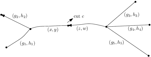
Refer to caption
Figure 15. We usually do not draw surface and just draw the graph

This gives a visual presentation of the parameterization of our GG-cover of extended surface with one or gluing of several standard blocks.

4. Moves

At this point, we want to remind our readers about our main goal of this paper. we will eventually define a 22-dimensional CW complex M⁡(Σ~,Σ)M(\tilde{\Sigma},\Sigma), which has the set of all parameterization of Σ~\tilde{\Sigma} as the set of vertices. The edges of M⁡(Σ~,Σ)M(\tilde{\Sigma},\Sigma) will be directed; we call them moves. It is convenient to look at M⁡(Σ~,Σ)M(\tilde{\Sigma},\Sigma) as a groupoid with objects—all vertices and morphisms between two vertices—the set of homotopy classes of paths on the edges of M⁡(Σ~,Σ)M(\tilde{\Sigma},\Sigma) from the first vertex to the second one (going along an edge in the direction opposite to its orientation is allowed). We will use group notation writing a path composed of edges E1,E2,…E_{1},E_{2},\dots as a product E1​…​E2E_{1}\dots E_{2}, and we will write E−1E^{-1} if the edge EE is traveled in the opposite direction. Then the 22-cells are interpreted as relations among the moves: we will write E1⋯Ek=idE_{1}\cdots E_{k}=id if the closed loop formed by the edges E1,…,EkE_{1},\dots,E_{k} is contractible in M⁡(Σ~,Σ)M(\tilde{\Sigma},\Sigma); if we want to specify the base point for the loop, we will write E1⋯Ek(M)=id(M)E_{1}\cdots E_{k}(M)=id(M). We will write E:M→M′E:M\to M^{\prime} if the edge EE goes from MM to M′M^{\prime}.

Our Main Theorems state that the complex M⁡(Σ~,Σ)M(\tilde{\Sigma},\Sigma) is connected and simply-connected. This main theorem will be described in detail after we describe the moves or edges in this section.

4.1. Standard Morphism

Before describing our moves, we need to define some standard morphisms between our standard blocks. These are described in terms of lifting of certain morphisms between base surfaces SnS_{n}. These are:

z:Sn⟶Snz:S_{n}\longrightarrow S_{n}
b:S3⟶S3b:S_{3}\longrightarrow S_{3}
αk,l:Sk+1⊔Sl+1⟶Sk+l\alpha_{k,l}:S_{k+1}\sqcup S_{l+1}\longrightarrow S_{k+l}

For a more elaborate description of these morphism, see the paper [BK]. Here we will just give a quick description.

1:

zz is the rotation of the sphere which cyclically permutes the boundary circles. That is if mm is a marking on SnS_{n} then z⁡(m)z(m) will be the same marking (of course up to homotopy) on SnS_{n} but with a different distinguished edge. See the figure 16 where n=4n=4.

Refer to caption
Figure 16. A pictorial description of zz map for n=4n=4
2:

Now we will describe briefly the braiding, bb, see [BK] for detail. If we label the boundary circles of S3S_{3} by α,β,γ\alpha,\beta,\gamma, then sometimes we will denote by bα,βb_{\alpha,\beta} the braiding of the α\alpha and β\beta component of S3S_{3}. Let mm is the graph on S3S_{3} shown on the left hand side of figure 17. Then we define the bα,βb_{\alpha,\beta} by figure 17.

Refer to caption
Figure 17. Visual description of bb map
3:

αk,l\alpha_{k,l} is the identification of the result of gluing Sk+1S_{k+1} and Sl+1S_{l+1} (along the (k+1)(k+1) th boundary component of the first one with the 11 st boundary component of the last one) with, Sk+lS_{k+l}, the standard sphere with (k+l)(k+l) hole. For more detail description see [BK].

Lemma 8.

Each of the above defined morphisms between SnS_{n} (n=3n=3 in the case of bb) can be uniquely lifted to the GG-cover of SnS_{n}, Sn(g1,….gn;h1,…hn)S_{n}(g_{1},....g_{n};h_{1},...h_{n}), described by:

z~:Sn​(g1​…​gn,h1​…​hn)⟶Sn​(gn,g1​…​gn−1,hn,h1​…​hn−1)\tilde{z}:S_{n}(g_{1}...g_{n};h_{1}...h_{n})\longrightarrow S_{n}(g_{n},g_{1}...g_{n-1};h_{n},h_{1}...h_{n-1})
b~:S3​(g1,g2,g3,h1,h2,h3)⟶S3​(g1​g2​g1−1,g1,g3,h2​g1−1,h1,h3)\tilde{b}:S_{3}(g_{1},g_{2},g_{3};h_{1},h_{2},h_{3})\longrightarrow S_{3}(g_{1}g_{2}g_{1}^{-1},g_{1},g_{3};h_{2}g_{1}^{-1},h_{1},h_{3})
αk,l~:Sk+1​(𝐠,𝐡)⊔Sl+1​(𝐠′,𝐡′)⟶Sk+l​(𝐠′′,𝐡′′)\tilde{\alpha_{k,l}}:S_{k+1}(\mathbf{g},\mathbf{h})\sqcup S_{l+1}(\mathbf{g^{\prime}},\mathbf{h^{\prime}})\longrightarrow S_{k+l}(\mathbf{g^{\prime\prime}},\mathbf{h^{\prime\prime}})

where

𝐠\displaystyle\mathbf{g} =\displaystyle= (g1​…​gk+1)\displaystyle(g_{1}...g_{k+1})
𝐡\displaystyle\mathbf{h} =\displaystyle= (h1​…​hk+1)\displaystyle(h_{1}...h_{k+1})
𝐠′\displaystyle\mathbf{g^{\prime}} =\displaystyle= (g1′,…​gl+1′)\displaystyle(g_{1}^{\prime},...g_{l+1}^{\prime})
𝐡′\displaystyle\mathbf{h^{\prime}} =\displaystyle= (h1′,…​hl+1′)\displaystyle(h_{1}^{\prime},...h_{l+1}^{\prime})

So that hk+1​gk+1−1​hk+1−1=[h1′​g1′−1​h1′−1]−1;hk+1=h1′h_{k+1}g_{k+1}^{-1}h_{k+1}^{-1}=[h_{1}^{\prime}g_{1}^{\prime-1}h_{1}^{\prime-1}]^{-1};h_{k+1}=h_{1}^{\prime}
And

𝐠′′\displaystyle\mathbf{g^{\prime\prime}} =\displaystyle= (g1​…​gk,g2′​…​gl+1′)\displaystyle(g_{1}...g_{k},g_{2}^{\prime}...g_{l+1}^{\prime})
𝐡′′\displaystyle\mathbf{h^{\prime\prime}} =\displaystyle= (h1​…​hk,h2′​…​hl+1′)\displaystyle(h_{1}...h_{k},h_{2}^{\prime}...h_{l+1}^{\prime})
Remark 5.

Notice that we need hk+1​gk+1−1​hk+1−1=[h1′​g1′−1​h1′−1]−1h_{k+1}g_{k+1}^{-1}h_{k+1}^{-1}=[h_{1}^{\prime}g_{1}^{\prime-1}h_{1}^{\prime-1}]^{-1} so that it is possible to glue the (k+1)(k+1) th boundary circle of Sk+1S_{k+1} with 11st boundary circle of Sl+1S_{l+1}. This is to make sure that the monodromy (see 2.6.1 on page 2.6.1) of (k+1)(k+1) th boundary circle of Sk+1S_{k+1} is inverse of the monodromy of 11st boundary circle of Sl+1S_{l+1} (recall that the orientation of two boundary circles must be opposite for glue to exist). The second equality, hk+1=h1′h_{k+1}=h_{1}^{\prime}, is an extra one which is not needed for the gluing to exist but we assume this extra condition whenever we want to apply αk,l~\tilde{\alpha_{k,l}}.

Proof.

First consider the GG-covers,Sn​(g1​…​gn,h1​…​hn)S_{n}(g_{1}...g_{n};h_{1}...h_{n}) and Sn​(gn,g1​…​gn−1,hn,h1​…​hn−1)S_{n}(g_{n},g_{1}...g_{n-1};h_{n},h_{1}...h_{n-1}), and the map z:Sn⟶Snz:S_{n}\longrightarrow S_{n}. Our base surface, SnS_{n} has genus zero and the map zz preserves the monodromy which can be easily checked by hand. So according to lemma 2 (see 2 on page 2), this map zz can be uniquely lifted to the GG-cover. Similarly, in all the other cases, all we have to check that the maps b:S3⟶S3b:S_{3}\longrightarrow S_{3} and αk,l:Sk+1⊔Sl+1⟶Sk+l\alpha_{k,l}:S_{k+1}\sqcup S_{l+1}\longrightarrow S_{k+l} preserve the monodromy. This can be easily checked by hand, using the lemma 6. ∎

4.1.1. The standard morphism, ϕx,x∈G\phi_{x},x\in G

This is just a reminder to the reader. We have already defined ϕx\phi_{x} move before. This is the morphism between standard blocks defined by
ϕx\phi_{x} : Sn​(g1​…​gn,h1​…​hn)⟶Sn​(x​g1​x−1​…​x​gn​x−1,h1​x−1​…​hn​x−1)S_{n}(g_{1}...g_{n};h_{1}...h_{n})\longrightarrow S_{n}(xg_{1}x^{-1}...xg_{n}x^{-1};h_{1}x^{-1}...h_{n}x^{-1}). See lemma 4 on page 4.

4.2. 𝐙\mathbf{Z}, 𝐁\mathbf{B} ,and 𝐅\mathbf{F} Move

For |G|=1|G|=1, these moves are described in the paper [BK]. Reader might want to read this first before continue. We again want to remind our readers that our base surface will always have genus 0, unless otherwise specified. We will first have three moves similar to the ZZ, BB and FF moves of the paper [BK]. These moves will be called 𝐙\mathbf{Z}-move, 𝐁\mathbf{B}-move and 𝐅\mathbf{F}-move respectively. Note that we use boldface letter to denote these three moves so that it does not get confused with the ZZ, BB, and FF moves of the paper [BK]. Then we will have two extra moves which do not have any correspondence to the paper [BK]. So again ZZ, BB and FF will denote the moves in the case of |G|=1|G|=1 and 𝐙\mathbf{Z}, 𝐁\mathbf{B} ,and 𝐅\mathbf{F} will denote the moves in the general case. Each move will take a parameterization to another parameterization. So let us start describing these moves in more detail:

4.2.1. 𝐙\mathbf{Z} move

Given a GG-cover (π~:Σ~⟶Σ,{pa~})(\tilde{\pi}:\tilde{\Sigma}\longrightarrow\Sigma,\{\tilde{p_{a}}\}) of (Σ,{pa})(\Sigma,\{p_{a}\}), and a parameterization of this GG-cover with a standard block. This means we have an isomorphism, ff, of this GG-cover with one of the standard block say Sn​(g1​…​gn,h1​…​hn)S_{n}(g_{1}...g_{n};h_{1}...h_{n}). 𝐙\mathbf{Z} move takes this parameterization ff to the parameterization z~∘f\tilde{z}\circ f where z~\tilde{z} is the standard morphism defined in the lemma 5. This new parameterization identify the original GG-cover with Sn​(gn,g1​…​gn−1,hn,h1​…​hn−1)S_{n}(g_{n},g_{1}...g_{n-1};h_{n},h_{1}...h_{n-1}). Look at the diagram below

    Original G-cover    f         Sn​(g1​…​gn,h1​…​hn)    z~         Sn​(gn,g1​…​gn−1,hn,h1​…​hn−1)    ⏟z~∘f=𝐙⁡(f), 𝐙 move applied to f\underbrace{\lx@xy@svg{\hbox{\raise 2.5pt\hbox{\kern 39.31256pt\hbox{\ignorespaces\ignorespaces\ignorespaces\hbox{\vtop{\halign{\entry@#!@&&\entry@@#!@\cr&&\crcr}}}\ignorespaces{\hbox{\kern-39.31256pt\raise 0.0pt\hbox{\hbox{\kern 0.0pt\raise 0.0pt\hbox{\hbox{\kern 3.0pt\raise-2.5pt\hbox{$\textstyle{\mbox{Original G-cover}\ignorespaces\ignorespaces\ignorespaces\ignorespaces}$}}}}}}}\ignorespaces\ignorespaces\ignorespaces\ignorespaces{}{\hbox{\lx@xy@droprule}}\ignorespaces\ignorespaces\ignorespaces{\hbox{\kern 50.98407pt\raise 6.1111pt\hbox{{}\hbox{\kern 0.0pt\raise 0.0pt\hbox{\hbox{\kern 3.0pt\hbox{\hbox{\kern 0.0pt\raise-1.75pt\hbox{$\scriptstyle{f}$}}}\kern 3.0pt}}}}}}\ignorespaces{\hbox{\kern 63.31256pt\raise 0.0pt\hbox{\hbox{\kern 0.0pt\raise 0.0pt\hbox{\lx@xy@tip{1}\lx@xy@tip{-1}}}}}}{\hbox{\lx@xy@droprule}}{\hbox{\lx@xy@droprule}}{\hbox{\kern 63.31256pt\raise 0.0pt\hbox{\hbox{\kern 0.0pt\raise 0.0pt\hbox{\hbox{\kern 3.0pt\raise-2.5pt\hbox{$\textstyle{S_{n}(g_{1}...g_{n};h_{1}...h_{n})\ignorespaces\ignorespaces\ignorespaces\ignorespaces}$}}}}}}}\ignorespaces\ignorespaces\ignorespaces\ignorespaces{}{\hbox{\lx@xy@droprule}}\ignorespaces\ignorespaces\ignorespaces{\hbox{\kern 179.22076pt\raise 6.61111pt\hbox{{}\hbox{\kern 0.0pt\raise 0.0pt\hbox{\hbox{\kern 3.0pt\hbox{\hbox{\kern 0.0pt\raise-3.61111pt\hbox{$\scriptstyle{\tilde{z}}$}}}\kern 3.0pt}}}}}}\ignorespaces{\hbox{\kern 185.99188pt\raise 0.0pt\hbox{\hbox{\kern 0.0pt\raise 0.0pt\hbox{\lx@xy@tip{1}\lx@xy@tip{-1}}}}}}{\hbox{\lx@xy@droprule}}{\hbox{\lx@xy@droprule}}{\hbox{\kern 185.99188pt\raise 0.0pt\hbox{\hbox{\kern 0.0pt\raise 0.0pt\hbox{\hbox{\kern 3.0pt\raise-2.5pt\hbox{$\textstyle{S_{n}(g_{n},g_{1}...g_{n-1};h_{n},h_{1}...h_{n-1})}$}}}}}}}\ignorespaces}}}}\ignorespaces}_{\tilde{z}\circ f=\mathbf{Z}(f),\mbox{ $\mathbf{Z}$ move applied to f}}

4.2.2. 𝐁\mathbf{B} move

Given a GG-cover (π~:Σ~⟶Σ,{pa~})(\tilde{\pi}:\tilde{\Sigma}\longrightarrow\Sigma,\{\tilde{p_{a}}\}) of (Σ,{pa})(\Sigma,\{p_{a}\}), and a parameterization of this GG-cover with a standard block, S3​(g1,g2,g3,h1,h2,h3)S_{3}(g_{1},g_{2},g_{3};h_{1},h_{2},h_{3}). This means we have an isomorphism,ff, of this GG-cover with S3​(g1,g2,g3,h1,h2,h3)S_{3}(g_{1},g_{2},g_{3};h_{1},h_{2},h_{3}). 𝐁\mathbf{B} move takes this parameterization ff to the parameterization b~∘f\tilde{b}\circ f where b~\tilde{b} is the standard morphism defined in the lemma 8. This new parameterization identify the original GG-cover with S3​(g1​g2​g1−1,g1,g3,h2​g1−1,h1,h3)S_{3}(g_{1}g_{2}g_{1}^{-1},g_{1},g_{3};h_{2}g_{1}^{-1},h_{1},h_{3}).

4.2.3. 𝐅\mathbf{F} move

Here the setup is a little different from the above two moves. Fist, let Σ\Sigma be an extended surface of genus 00 with one cut {c}\{c\}. This cut {cc} divides Σ\Sigma into two pieces. Say, GG-cover of one piece is parameterized with Sk+1​(𝐠,𝐡)S_{k+1}(\mathbf{g},\mathbf{h}) and the other with Sl+1(𝐠′,𝐡′)S_{l+1}(\mathbf{g^{{}^{\prime}}},\mathbf{h^{{}^{\prime}}}). That is the parameterization, ff, is given by:

f:Σ~⟶Sk+1(𝐠,𝐡)⨆c,hk+1Sl+1(𝐠′,𝐡′)f:\tilde{\Sigma}\longrightarrow S_{k+1}(\mathbf{g},\mathbf{h})\bigsqcup_{c,h_{k+1}}S_{l+1}(\mathbf{g^{{}^{\prime}}},\mathbf{h^{{}^{\prime}}})

where

𝐠\displaystyle\mathbf{g} =\displaystyle= (g1​…​gk+1)\displaystyle(g_{1}...g_{k+1})
𝐡\displaystyle\mathbf{h} =\displaystyle= (h1​…​hk+1)\displaystyle(h_{1}...h_{k+1})
𝐠′\displaystyle\mathbf{g^{\prime}} =\displaystyle= (g1′,…​gl+1′)\displaystyle(g_{1}^{\prime},...g_{l+1}^{\prime})
𝐡′\displaystyle\mathbf{h^{\prime}} =\displaystyle= (h1′,…​hl+1′)\displaystyle(h_{1}^{\prime},...h_{l+1}^{\prime})

And also hk+1​gk+1−1​hk+1−1=[h1′​g1′−1​h1′−1]−1;hk+1=h1′h_{k+1}g_{k+1}^{-1}h_{k+1}^{-1}=[h_{1}^{\prime}g_{1}^{\prime-1}h_{1}^{\prime-1}]^{-1};h_{k+1}=h_{1}^{\prime}
Thus the parameterization of the whole GG-cover, ff, identifies the GG-cover with the result of gluing these two standard blocks along the k+1k+1 st boundary circle of one side with the 11st boundary circle of the other. See the picture on figure 18 for more detail.

Refer to caption
Figure 18. Visual description of the parameterization of ff

Now by applying 𝐅\mathbf{F} move to ff, we get a new parameterization αk.l~∘f\tilde{\alpha_{k.l}}\circ f. Note that, αk.l~∘f\tilde{\alpha_{k.l}}\circ f is a parameterization of G-cover of Σ\Sigma with no cuts with Sk+l​(𝐠′′,𝐡′′)S_{k+l}(\mathbf{g^{\prime\prime}},\mathbf{h^{\prime\prime}}) where

𝐠′′\displaystyle\mathbf{g^{\prime\prime}} =\displaystyle= (g1​…​gk,g2′​…​gl+1′)\displaystyle(g_{1}...g_{k},g_{2}^{\prime}...g_{l+1}^{\prime})
𝐡′′\displaystyle\mathbf{h^{\prime\prime}} =\displaystyle= (h1​…​hk,h2′​…​hl+1′).\displaystyle(h_{1}...h_{k},h_{2}^{\prime}...h_{l+1}^{\prime}).

See the figure 19.

Refer to caption
Figure 19. Visualization of the parameterization 𝐅⁡(f)\mathbf{F}(f)
Remark 6.

If two components are glued along a cut where the edges corresponding to this cut are labeled by (x,y)(x,y) and (z,w)(z,w), then for this gluing to exist, we must have

x​y−1​x−1=[z​w−1​z−1]−1xy^{-1}x^{-1}=[zw^{-1}z^{-1}]^{-1}

See subsection 3.5 on page 3.5 for more detail explanation. Now to apply 𝐅\mathbf{F} move to this cut, we also required the extra condition that y=wy=w. This will imply that x​z=1xz=1. The requirement, y=wy=w, is not necessary for gluing to exist but we only require this whenever we want to apply 𝐅\mathbf{F} move to a cut.

A remark about notation: Note that by applying a 𝐅\mathbf{F} move, we are removing a cut. If the cut for one component is labeled by (x,y)(x,y) then the cut for the other component must be labeled by (x−1,y)(x^{-1},y) for 𝐅\mathbf{F} move to apply. See the picture on figure 20.

Refer to caption
Figure 20.

This x∈Gx\in G is completely determined by the label of all the other cuts since they all must multiplied to 1∈G1\in G. But for the second component yy, we have a choice. So it is better to encode the cut cc and the label yy in the notation. From now on, a 𝐅\mathbf{F} move will always be denoted by 𝐅𝐜,𝐲\mathbf{F_{c,y}} to emphasize the cut, cc, and the choice of point, yy.

4.3. 𝐏𝐱\mathbf{P_{x}}-move where x∈Gx\in G

Beside 𝐙\mathbf{Z}, 𝐁\mathbf{B} and 𝐅\mathbf{F} move, we need one more move which we will denote by 𝐏𝐱\mathbf{P_{x}} where x∈Gx\in G. This 𝐏𝐱\mathbf{P_{x}}-move is defined in the following way:
Given a GG-cover (π~:Σ~⟶Σ,{pa~})(\tilde{\pi}:\tilde{\Sigma}\longrightarrow\Sigma,\{\tilde{p_{a}}\}) of (Σ,{pa})(\Sigma,\{p_{a}\}), and a parameterization of this GG-cover with a standard block. This means we have an isomorphism, ff, of this GG-cover with one of the standard block say Sn​(g1​…​gn,h1​…​hn)S_{n}(g_{1}...g_{n};h_{1}...h_{n}). 𝐏𝐱\mathbf{P_{x}} move takes this parameterization ff to the parameterization ϕx∘f\phi_{x}\circ f where ϕx\phi_{x} is the morphism defined by
ϕx\phi_{x} : Sn​(g1​…​gn,h1​…​hn)⟶Sn​(x​g1​x−1​…​x​gn​x−1,h1​x−1​…​hn​x−1)S_{n}(g_{1}...g_{n};h_{1}...h_{n})\longrightarrow S_{n}(xg_{1}x^{-1}...xg_{n}x^{-1};h_{1}x^{-1}...h_{n}x^{-1}). See the lemma 4 for the description of ϕ⁡(x)\phi(x). See the diagram below:

Σ~→fSn(g1….gn;h1…hn)→ϕxSn(xg1x−1…xgnx−1;h1x−1…hnx−1)\tilde{\Sigma}\stackrel{{\scriptstyle f}}{{\rightarrow}}S_{n}(g_{1}....g_{n};h_{1}...h_{n})\stackrel{{\scriptstyle\phi_{x}}}{{\rightarrow}}S_{n}(xg_{1}x^{-1}...xg_{n}x^{-1};h_{1}x^{-1}...h_{n}x^{-1})
ϕx∘f=𝐏x​(f)\phi_{x}\circ f=\mathbf{P}_{x}(f)

4.4. 𝐓𝐳,𝐲𝐜\mathbf{T_{z,y}^{c}} move

Say we have the following parameterization, ff, of our GG-cover:

f:Σ~⟶Sn​(g1​…​gn−1,x,h1​…​hn−1,y)​⨆c,ySm​(x−1,u1​…​um−1,y,v1​…​vm−1)f:\tilde{\Sigma}\longrightarrow S_{n}(g_{1}...g_{n-1},x;h_{1}...h_{n-1},y)\bigsqcup_{c,y}S_{m}(x^{-1},u_{1}...u_{m-1};y,v_{1}...v_{m-1})

cc is the cut where we glue the two components. Note that all conditions are satisfied so that the gluing make sense. Here xx is determine by all the other element, namely, x=(g1​…​gn−1)−1=(u1​…​um−1)−1x=(g_{1}...g_{n-1})^{-1}=(u_{1}...u_{m-1})^{-1}, but yy is not determine; we can choose yy freely. By definition, 𝐓𝐳,𝐲𝐜𝐢​(f)\mathbf{T_{z,y}^{c_{i}}}(f) is the following parameterization:

𝐓𝐳,𝐲𝐜(f):Σ~→Sn(g1..gn−1,x;h1..hn−1,z)⨆c,ySm(x−1,u1..um−1;z,v1..vm−1)\mathbf{T_{z,y}^{c}}(f):\tilde{\Sigma}\rightarrow S_{n}(g_{1}..g_{n-1},x;h_{1}..h_{n-1},z)\bigsqcup_{c,y}S_{m}(x^{-1},u_{1}..u_{m-1};z,v_{1}..v_{m-1})

Where we replace the choice of `​`​y​"``y" with the choice of `​`​z​"``z".

Remark 7.

Although we introduce this new move, 𝐓𝐳,𝐲𝐜\mathbf{T_{z,y}^{c}}, this can in fact be thought of as composition of two 𝐅\mathbf{F} move. Namely 𝐓𝐳,𝐲𝐜=𝐅𝐜,𝐳−𝟏​𝐅𝐜,𝐲\mathbf{T_{z,y}^{c}}=\mathbf{F_{c,z}^{-1}F_{c,y}}. The move, 𝐅𝐜,𝐲\mathbf{F_{c,y}}, will remove the cut, cc, with the choice of point yy, while the move 𝐅𝐜,𝐳−𝟏\mathbf{F_{c,z}^{-1}} will replace the cut, cc, but this time with the choice of point zz. The reason for introducing such an extra move will be clear later, but introducing this new move 𝐓𝐳,𝐲𝐜\mathbf{T_{z,y}^{c}} and adding the relation 𝐓𝐳,𝐲𝐜=𝐅𝐜,𝐳−𝟏​𝐅𝐜,𝐲\mathbf{T_{z,y}^{c}}=\mathbf{F_{c,z}^{-1}F_{c,y}} will not do any harm, since one can easily sees that the complex M⁡(Σ~,Σ)M(\tilde{\Sigma},\Sigma) without the 𝐓𝐳,𝐲𝐜\mathbf{T_{z,y}^{c}} move and 𝐓𝐳,𝐲𝐜=𝐅𝐜,𝐳−𝟏​𝐅𝐜,𝐲\mathbf{T_{z,y}^{c}}=\mathbf{F_{c,z}^{-1}F_{c,y}} relation is connected and simply-connected iff the complex M⁡(Σ~,Σ)M(\tilde{\Sigma},\Sigma) with the 𝐓𝐳,𝐲𝐜\mathbf{T_{z,y}^{c}} move and 𝐓𝐳,𝐲𝐜=𝐅𝐜,𝐳−𝟏​𝐅𝐜,𝐲\mathbf{T_{z,y}^{c}}=\mathbf{F_{c,z}^{-1}F_{c,y}} relation is connected and simply-connected.

See the picture on figure 21 for a visual description of 𝐓\mathbf{T} move.

Refer to caption
Figure 21. The sequence of diagram describing 𝐓\mathbf{T} move

4.5. Moves, when more than one standard blocks are glued together

Let Σ~\tilde{\Sigma} be a GG cover of Σ\Sigma. Also let ff be a parameterization of this GG cover with gluing of several standard blocks. In other word,

f:Σ~→Sn1​(𝐠𝟏,𝐡𝟏)​⨆g​l​u​e​dSn2​(𝐠𝟐,𝐡𝟐)​⨆g​l​u​e​d…..⨆g​l​u​e​dSnk​(𝐠𝐤,𝐡𝐤)f:\tilde{\Sigma}\rightarrow S_{n_{1}}(\mathbf{g_{1},h_{1}})\bigsqcup_{glued}S_{n_{2}}(\mathbf{g_{2},h_{2}})\bigsqcup_{glued}.....\bigsqcup_{glued}S_{n_{k}}(\mathbf{g_{k},h_{k}})

This parameterization of ff, by the restriction on each component, can be realized as a gluing of kk parameterization. That is f=f1⊔f2⊔…..⊔fkf=f_{1}\sqcup f_{2}\sqcup.....\sqcup f_{k}. Let 𝐄\mathbf{E} be one of the above five moves, that is 𝐄∈𝐙,𝐁,𝐅,𝐏𝐱,𝐓\mathbf{E}\in\mathbf{Z,B,F,P_{x},T}. Then by the move i​d⊔i​d⊔….⊔𝐄⊔…⊔i​did\sqcup id\sqcup....\sqcup\mathbf{E}\sqcup...\sqcup id(ff), where 𝐄\mathbf{E} appears in the iith component, we mean that we only apply 𝐄\mathbf{E} move to the fif_{i} parameterization and identity to all others. An example of such a move is shown on figure 22. For simplicity of the picture, we take three components.

Refer to caption
Figure 22. An example of a move when having more than one component.

4.6. 𝐁𝐢\mathbf{B_{i}} move

The 𝐁\mathbf{B} move is very restricted; it is only defined for n=3n=3. So we need a little flexibility. This 𝐁𝐢\mathbf{B_{i}} move will be a braiding of ii and i+1i+1 boundary circles. This is in fact not a new move but a composition of previously defined moves. This will be used many times from now on when we will describe the other moves and relation. So it is important to do this right now. Let ff be a parameterization of a GG cover, Σ~\tilde{\Sigma}, with a standard block say Sn​(g1,…,gn,h1,…,hn)S_{n}(g_{1},...,g_{n};h_{1},...,h_{n}). Then 𝐁𝐢\mathbf{B_{i}} is the composition of the moves described in the figure 23. Here we only draw pictures for n=6n=6 for convenience but readers are clear of what should be done for other nn. If

Σ~→fSn​(g1,…,gn,h1,…,hn)\tilde{\Sigma}\stackrel{{\scriptstyle f}}{{\rightarrow}}S_{n}(g_{1},...,g_{n};h_{1},...,h_{n})

Then

Σ~→𝐁𝐢​(f)Sn(g1,..,gi−1,gigi+1gi−1,gi,…,gn;h1,..,hi−1,hi+1gi−1,hi,..,hn)\tilde{\Sigma}\stackrel{{\scriptstyle\mathbf{B_{i}}(f)}}{{\rightarrow}}S_{n}(g_{1},..,g_{i-1},g_{i}g_{i+1}g_{i}^{-1},g_{i},...,g_{n};h_{1},..,h_{i-1},h_{i+1}g_{i}^{-1},h_{i},..,h_{n})
Refer to caption
Figure 23. description of 𝐁𝐢\mathbf{B_{i}} move as a composition of previously defined move

5. The Complex

5.1. Definition of the complex M⁡(Σ~,Σ)M(\tilde{\Sigma},\Sigma)

We are given a fixed GG-cover, Π:Σ~⟶Σ\Pi:\tilde{\Sigma}\longrightarrow\Sigma, where Σ\Sigma will always denote an extended surface which is compact, orientable, closed surface of genus zero unless otherwise specified. We will first define the 11-skeleton of the complex, M⁡(Σ~,Σ)M(\tilde{\Sigma},\Sigma), that is the vertex and the edges.
{The set of vertex of M⁡(Σ~,Σ)M(\tilde{\Sigma},\Sigma)} = {The set of parameterization of the GG-cover Π:Σ~⟶Σ\Pi:\tilde{\Sigma}\longrightarrow\Sigma}
A vertex, α\alpha, is connected to vertex β\beta, directed from α\alpha to β\beta, if β\beta can be obtained from α\alpha by applying one of the following moves:
𝐙,𝐙−𝟏,𝐁𝐢,𝐁𝐢−𝟏,𝐅,𝐅−𝟏,𝐏𝐱,𝐏𝐱−𝟏,𝐓𝐳,𝐲𝐜,(𝐓𝐳,𝐲𝐜)−𝟏\mathbf{Z,Z^{-1},B_{i},B_{i}^{-1},F,F^{-1},P_{x},P_{x}^{-1},\mathbf{T_{z,y}^{c}},(\mathbf{T_{z,y}^{c}})^{-1}} in one of the components. Having defined the vertex and edges of the complex M⁡(Σ~,Σ)M(\tilde{\Sigma},\Sigma) , now we need to define the relations or 2-cells of M⁡(Σ~,Σ)M(\tilde{\Sigma},\Sigma). We define the relations in the next section.

5.2. The Statement Of the Main Theorem

Main Theorem.

The complex, M⁡(Σ~,Σ)M(\tilde{\Sigma},\Sigma), with the above defined edges and relations (which will be described in the next section), is connected and simply connected.

6. Relations

Now it is time to define all the relations between these moves. These relation will be described in the following subsections:

6.1. Obvious Relation

𝐄𝐄−𝟏=𝐄−𝟏​𝐄=1\mathbf{EE^{-1}}=\mathbf{E^{-1}E}=1

Where 𝐄\mathbf{E} is one of the five moves, that is 𝐄∈{𝐙,𝐁𝐢,𝐅,𝐏𝐱,𝐓𝐳,𝐲𝐜}\mathbf{E\in\{Z,B_{i},F,P_{x},T_{z,y}^{c}\}}

6.2. 𝐏𝐱\mathbf{P_{x}} Relation

𝐏𝐱\mathbf{P_{x}} move commutes with all the other moves. More precisely for all x,y∈Gx,y\in G and all cuts, cc, we have the following relations:

  1. (1)

    𝐏𝐱​𝐙=𝐙𝐏𝐱\mathbf{P_{x}Z}=\mathbf{ZP_{x}}

  2. (2)

    𝐏𝐱​𝐁𝐢=𝐁𝐢​𝐏𝐱\mathbf{P_{x}B_{i}}=\mathbf{B_{i}P_{x}}

  3. (3)

    𝐏𝐱​𝐅𝐜,𝐲=𝐅𝐜,𝐲𝐱−𝟏​(𝐏𝐱⊔𝐏𝐱)\mathbf{P_{x}F_{c,y}}=\mathbf{F_{c,yx^{-1}}(P_{x}\sqcup P_{x})}. See figure 24.

  4. (4)

    𝐏𝐱​𝐏𝐲=𝐏𝐱𝐲\mathbf{P_{x}P_{y}}=\mathbf{P_{xy}}

Remark 8.

Note the change of indices for 𝐅\mathbf{F}. Why we need to change the indices is clear from figure 24. Here we only label the edges corresponding to the cut cc.

Refer to caption
Figure 24. Visual description of the third 𝐏𝐱\mathbf{P_{x}} relation
Remark 9.

The last relation shows that whatever relation satisfied by the elements of GG, the same relation hold for 𝐏𝐱\mathbf{P_{x}}. So in particular this implies (𝐏𝐱)−𝟏=𝐏𝐱−𝟏\mathbf{(P_{x})^{-1}}=\mathbf{P_{x^{-1}}}.

6.3. 𝐏−𝐅\mathbf{P-F} relation

Let ff be a parameterization having two component glued to a cut cc where one edge of the cut labeled by (x,y)(x,y) and the other edge of the cut labeled by (z,w)(z,w). For this glue to exist, we must have y​x−1​y−1=[w​z−1​w−1]−1yx^{-1}y^{-1}=[wz^{-1}w^{-1}]^{-1}, see the subsection 3.5 on page 3.5. Let t=w−1​yt=w^{-1}y. Then one can easily check that t​x​t−1=z−1txt^{-1}=z^{-1}, y​t−1=wyt^{-1}=w, t−1​z​t=x−1t^{-1}zt=x^{-1} and w​t=ywt=y. Then 𝐏−𝐅\mathbf{P-F} relation is the following relation://

𝐅𝐜,𝐰​(𝐏𝐭⊔𝐢𝐝)=𝐅𝐜,𝐲​(𝐢𝐝⊔𝐏𝐭−𝟏)\mathbf{F_{c,w}(P_{t}\sqcup id)}=\mathbf{F_{c,y}(id\sqcup P_{t^{-1}})}

See the figure 25 for a visual description of this relation.

Refer to caption
Figure 25. Visual description of 𝐏−𝐅\mathbf{P-F} relation

6.4. 𝐙\mathbf{Z} Relation

𝐙\mathbf{Z} commutes with all the other moves. More precisely, let a parameterization, ff, identifies a GG cover,Σ~\tilde{\Sigma}, with the standard block Sn​(g1,…,gn,h1,…,hn)S_{n}(g_{1},...,g_{n};h_{1},...,h_{n}). Then we have the following relation:

𝐙𝐁𝐢=𝐁𝐢+𝟏​𝐙\mathbf{ZB_{i}}=\mathbf{B_{i+1}Z}

See figure 26 for a visual description of this relation.

Refer to caption
Figure 26. Notice the change of indices for 𝐁\mathbf{B}.

Also let a parameterization, ff, identifies a GG cover, Σ~\tilde{\Sigma}, with gluing of two standard blocks along a cut cc.

f:Σ~→Sn​(g1,…,gn−1,x,h1,…,hn−1,y)​⨆c,ySm​(x−1,g1′,…,gm−1′,y,h1′,…,hm−1′)f:\tilde{\Sigma}\rightarrow S_{n}(g_{1},...,g_{n-1},x;h_{1},...,h_{n-1},y)\bigsqcup_{c,y}S_{m}(x^{-1},g_{1}^{\prime},...,g_{m-1}^{\prime};y,h_{1}^{\prime},...,h_{m-1}^{\prime})

Then we have the following relation:

(i​d⊔𝐙)​𝐓𝐳,𝐲𝐜=𝐓𝐳,𝐲𝐜​(i​d⊔𝐙)(id\sqcup\mathbf{Z})\mathbf{T^{c}_{z,y}}=\mathbf{T^{c}_{z,y}}(id\sqcup\mathbf{Z})

See figure 27 for a visual description of this relation.

Refer to caption
Figure 27. The commutativity of 𝐙\mathbf{Z} and 𝐓\mathbf{T} moves

6.5. 𝐁\mathbf{B} Relation

From above relations, we already know that 𝐁\mathbf{B} move commutes with 𝐙\mathbf{Z} and 𝐏𝐱\mathbf{P_{x}} move. But we have more–𝐁\mathbf{B} also commutes with the 𝐓\mathbf{T} move. More precisely, let a parameterization, ff, identifies a GG cover,Σ~\tilde{\Sigma}, with gluing of two standard blocks where one of the standard blocks has three boundary circles.

f:Σ~→Sn​(g1,…,gn−1,x,h1,…,hn−1,y)​⨆c,yS3​(x−1,g1′,g2′,y,h1′,h2′)f:\tilde{\Sigma}\rightarrow S_{n}(g_{1},...,g_{n-1},x;h_{1},...,h_{n-1},y)\bigsqcup_{c,y}S_{3}(x^{-1},g_{1}^{\prime},g_{2}^{\prime};y,h_{1}^{\prime},h_{2}^{\prime})

Here cc denotes the cut where these two standard blocks are glued together. Then we have the following relation:

(i​d⊔𝐁)​𝐓𝐳,𝐲𝐜=𝐓𝐳,𝐲𝐜​(i​d⊔𝐁)(id\sqcup\mathbf{B})\mathbf{T^{c}_{z,y}}=\mathbf{T^{c}_{z,y}}(id\sqcup\mathbf{B})

See figure 28 where for simplicity we take n=4n=4.

Refer to caption
Figure 28. The commutativity of 𝐁\mathbf{B} and 𝐓\mathbf{T} moves

6.6. 𝐓𝐳,𝐲𝐜\mathbf{T_{z,y}^{c}} relation

This is simply the relation 𝐓𝐳,𝐲𝐜=𝐅𝐜,𝐳−𝟏​𝐅𝐜,𝐲\mathbf{T_{z,y}^{c}}=\mathbf{F_{c,z}^{-1}F_{c,y}} which is expected.

6.7. Rotation axiom

Let f:Σ~⟶Sn​(g1​…​gn,h1​…​hn)f:\tilde{\Sigma}\longrightarrow S_{n}(g_{1}...g_{n};h_{1}...h_{n}) be a parameterization of the GG-cover, Σ~\tilde{\Sigma}. Then the rotation axiom says that if we apply 𝐙\mathbf{Z} move nn times to the parameterization, ff, we get back the same parameterization, ff. That is 𝐙𝐧​f=f\mathbf{Z^{n}}f=f or 𝐙𝐧=1\mathbf{Z^{n}}=1. See the diagram on figure 29.

Refer to caption
Figure 29. The 2-cell of 𝐙\mathbf{Z} relation, for n=3n=3

6.8. Commutativity of Disjoint Union

Let Σ=Σ1​⨆Σ2\Sigma=\Sigma_{1}\bigsqcup\Sigma_{2}. Then by restriction, the GG-cover Σ~⟶Σ\tilde{\Sigma}\longrightarrow\Sigma can be broken down into two pieces, say,
Σ1~⟶Σ1\tilde{\Sigma_{1}}\longrightarrow\Sigma_{1} and Σ2~⟶Σ2\tilde{\Sigma_{2}}\longrightarrow\Sigma_{2}.
Thus a parameterization of Σ~⟶Σ\tilde{\Sigma}\longrightarrow\Sigma can be realized as disjoint union of two parameterization, one for Σ1~⟶Σ1\tilde{\Sigma_{1}}\longrightarrow\Sigma_{1}, and the other for Σ2~⟶Σ2\tilde{\Sigma_{2}}\longrightarrow\Sigma_{2}. We can reformulate this statement in the language of complex. In this case, it means that if AA is a vertex of the complex M⁡(Σ~,Σ)M(\tilde{\Sigma},\Sigma), then AA can be written as A=(A1,A2)A=(A_{1},A_{2}) where A1A_{1} is a vertex of M⁡(Σ1~,Σ1)M(\tilde{\Sigma_{1}},\Sigma_{1}) and A2A_{2} is a vertex of M⁡(Σ2~,Σ2)M(\tilde{\Sigma_{2}},\Sigma_{2}). Let 𝐄𝐢\mathbf{E_{i}} be an edge of M⁡(Σi~,Σi)M(\tilde{\Sigma_{i}},\Sigma_{i}) directed from AiA_{i} to Ai′A^{\prime}_{i}, here i=1,2i=1,2. Then the commutativity of disjoint union is the following relation:

(i​d​⨆𝐄𝟐)​(𝐄𝟏​⨆i​d)=(𝐄𝟏​⨆i​d)​(i​d​⨆𝐄𝟐)(id\bigsqcup\mathbf{E_{2}})(\mathbf{E_{1}}\bigsqcup id)=(\mathbf{E_{1}}\bigsqcup id)(id\bigsqcup\mathbf{E_{2}})

See the diagram on figure 30 for a visual presentation.

Refer to caption
Figure 30. The 2-cell of commutativity of disjoint union

6.9. Symmetry of 𝐅\mathbf{F} Move

Let ff be the following parameterization of the GG-cover, Σ~\tilde{\Sigma},

f:Σ~⟶Sk+1​(g1,…​gk+1,h1,…​hk+1)​⨆c,hk+1Sl+1​(g1′,…​gl+1′,h1′,…​hl+1′)f:\tilde{\Sigma}\longrightarrow S_{k+1}(g_{1},...g_{k+1};h_{1},...h_{k+1})\bigsqcup_{c,h_{k+1}}S_{l+1}(g^{\prime}_{1},...g^{\prime}_{l+1};h^{\prime}_{1},...h^{\prime}_{l+1})

Here the symbol,

⨆c,hk+1\bigsqcup_{c,h_{k+1}}

means that we glued along the cut cc where the edges of the cut are labeled by (t,hk+1)(t,h_{k+1}) and (t−1,hk+1)(t^{-1},h_{k+1}). This tt is completely determined by all the other labels. More precisely we have the following:
The boundary component labeled by gk+1g_{k+1} of the standard block, Sk+1​(g1,…​gk+1,h1,…​hk+1)S_{k+1}(g_{1},...g_{k+1};h_{1},...h_{k+1}) is glued with the boundary component labeled by g1′g^{\prime}_{1} of the standard block Sl+1​(g1′,…​gl+1′,h1′,…​hl+1′)S_{l+1}(g^{\prime}_{1},...g^{\prime}_{l+1};h^{\prime}_{1},...h^{\prime}_{l+1}). of course we must have hk+1=h1′h_{k+1}=h^{\prime}_{1} and gk+1=(g1′)−1g_{k+1}=(g^{\prime}_{1})^{-1} for gluing to exist. From this parameterization, ff, we can get an another parameterization, jj, where

j:Σ~⟶Sl+1​(g2′,…,gl+1′,g1′,h2′,…,hl+1′,h1′)​⨆c,h1′Sk+1​(gk+1,g1,…,gk,hk+1,h1,…,hk)j:\tilde{\Sigma}\longrightarrow S_{l+1}(g^{\prime}_{2},...,g^{\prime}_{l+1},g^{\prime}_{1};h^{\prime}_{2},...,h^{\prime}_{l+1},h^{\prime}_{1})\bigsqcup_{c,h^{\prime}_{1}}S_{k+1}(g_{k+1},g_{1},...,g_{k};h_{k+1},h_{1},...,h_{k})

This is done by first interchange the component Sk+1​(g1,…​gk+1,h1,…​hk+1)S_{k+1}(g_{1},...g_{k+1};h_{1},...h_{k+1}) and Sl+1​(g1′,…,gl+1′,h1′,…,hl+1′)S_{l+1}(g^{\prime}_{1},...,g^{\prime}_{l+1};h^{\prime}_{1},...,h^{\prime}_{l+1}) and then we apply z~−1\tilde{z}^{-1} to Sl+1​(g1′,…,gl+1′,h1′,…,hl+1′)S_{l+1}(g^{\prime}_{1},...,g^{\prime}_{l+1};h^{\prime}_{1},...,h^{\prime}_{l+1}) and z~\tilde{z} to Sk+1​(g1,…,gk+1,h1,…,hk+1)S_{k+1}(g_{1},...,g_{k+1};h_{1},...,h_{k+1}) so that the boundary component labeled by g1′g^{\prime}_{1} becomes the last component of Sl+1​(g1′,…​gl+1′,h1′,…​hl+1′)S_{l+1}(g^{\prime}_{1},...g^{\prime}_{l+1};h^{\prime}_{1},...h^{\prime}_{l+1}) and the boundary component labeled by gk+1g_{k+1} becomes the first component of Sk+1​(g1,…​gk+1,h1,…​hk+1)S_{k+1}(g_{1},...g_{k+1};h_{1},...h_{k+1}). See Lemma 7 for the description of z~\tilde{z}
Now the symmetry of 𝐅\mathbf{F} move is the following relation:

𝐙𝐥𝐅𝐜,𝐡𝐤+𝟏(f)=𝐅𝐜,𝐡𝟏′(j)\mathbf{Z^{l}F_{c,h_{k+1}}}(f)=\mathbf{F_{c,h_{1}^{{}^{\prime}}}}(j)

Or in short, we can just say

𝐙𝐥𝐅𝐜,𝐡𝐤+𝟏=𝐅𝐜,𝐡𝟏′\mathbf{Z^{l}F_{c,h_{k+1}}}=\mathbf{F_{c,h_{1}^{{}^{\prime}}}}

Here cc is the cut where we glue the GG-cover. For the notation, Fc,hk+1F_{c,h_{k+1}}, see the remark on sec 6.2.3. In word, this relation just says that, we can first interchange the component, apply 𝐙\mathbf{Z} and 𝐙−𝟏\mathbf{Z^{-1}} move to the components and then apply 𝐅\mathbf{F} move or we can just first apply the 𝐅\mathbf{F} move and then apply some appropriate power of 𝐙\mathbf{Z} move.

6.10. Associativity of Cuts

Let ff be the following parameterization of the GG-cover Σ~\tilde{\Sigma}

f:Σ~→Sk+1(g1,..gk+1;h1,..hk+1)⨆c1,hk+1Sl+1(g1′,..gl+1′;h1′,..hl+1′)⨆c2,hl+1′Sn+1(g1′′,..gn+1′′;h1′′,..hn+1′′)f:\tilde{\Sigma}\rightarrow S_{k+1}(g_{1},..g_{k+1};h_{1},..h_{k+1})\bigsqcup_{c_{1},h_{k+1}}S_{l+1}(g^{\prime}_{1},..g^{\prime}_{l+1};h^{\prime}_{1},..h^{\prime}_{l+1})\bigsqcup_{c_{2},h^{\prime}_{l+1}}S_{n+1}(g^{\prime\prime}_{1},..g^{\prime\prime}_{n+1};h^{\prime\prime}_{1},..h^{\prime\prime}_{n+1})

For the description of the notation,

⨆c1,hk+1 and ⨆c2,hl+1′\bigsqcup_{c_{1},h_{k+1}}\mbox{ and }\bigsqcup_{c_{2},h^{\prime}_{l+1}}

see the relation“Symmetry of 𝐅\mathbf{F} move”. Here c1c_{1} denote the first cut and c2c_{2} denote the second cut of the gluing. Of course, we assume that all the conditions are satisfied for gluing to exist. More specifically, we assume the following conditions:
hk+1=h1′h_{k+1}=h^{\prime}_{1} , hl+1′=h1′′h^{\prime}_{l+1}=h^{\prime\prime}_{1} , gk+1​g1′=1g_{k+1}g^{\prime}_{1}=1 , gl+1′​g1′′=1g^{\prime}_{l+1}g^{\prime\prime}_{1}=1
Now the ”associativity of cuts” is the following relation:

𝐅𝐜𝟐,𝐡𝐥+𝟏′​𝐅𝐜𝟏,𝐡𝐤+𝟏​(f)=𝐅𝐜𝟏,𝐡𝐤+𝟏​𝐅𝐜𝟐,𝐡𝐥+𝟏′​(f)\mathbf{F_{c_{2},h^{\prime}_{l+1}}F_{c_{1},h_{k+1}}}(f)=\mathbf{F_{c_{1},h_{k+1}}F_{c_{2},h^{\prime}_{l+1}}}(f)

or in short, we can just say

𝐅𝐜𝟐,𝐡𝐥+𝟏′​𝐅𝐜𝟏,𝐡𝐤+𝟏=𝐅𝐜𝟏,𝐡𝐤+𝟏​𝐅𝐜𝟐,𝐡𝐥+𝟏′\mathbf{F_{c_{2},h^{\prime}_{l+1}}F_{c_{1},h_{k+1}}}=\mathbf{F_{c_{1},h_{k+1}}F_{c_{2},h^{\prime}_{l+1}}}

In word, this just says that, given two distinct cuts, it does not matter in which order we apply the 𝐅\mathbf{F} move.

6.11. Cylinder Axiom

We consider the standard cylinder (S2S_{2}) with the standard marking. See the picture on figure 31.

Refer to caption
Figure 31. Standard marking on S2S_{2}

Let f:Ω~⟶S2​(x,x−1,y,z)f:\tilde{\Omega}\longrightarrow S_{2}(x,x^{-1};y,z) be a parameterization of a GG-cover, Ω~→Ω\tilde{\Omega}\rightarrow\Omega. Also let jj be the following parameterization of GG-cover, Σ~→Σ\tilde{\Sigma}\rightarrow\Sigma:

j:Σ~⟶Sk+1​(g1,…,gk,x−1,h1,…,hk,y)j:\tilde{\Sigma}\longrightarrow S_{k+1}(g_{1},...,g_{k},x^{-1};h_{1},...,h_{k},y)

Note that, here we choose all the elements of GG in such a way that we can glue the G-cover Ω~\tilde{\Omega} and Σ~\tilde{\Sigma}. So after this gluing, we get a new parameterization of the GG-cover

Σ~​⨆g​l​u​e​dΩ~\tilde{\Sigma}\bigsqcup_{glued}\tilde{\Omega}

Let us denote this parameterization by j⊔fj\sqcup f. That is

j⊔f:Σ~​⨆g​l​u​e​dΩ~→Sk+1​(g1,…,gk,x−1,h1,…,hk,y)​⨆x−1,xS2​(x,x−1,y,z)j\sqcup f:\tilde{\Sigma}\bigsqcup_{glued}\tilde{\Omega}\rightarrow S_{k+1}(g_{1},...,g_{k},x^{-1};h_{1},...,h_{k},y)\bigsqcup_{x^{-1},x}S_{2}(x,x^{-1};y,z)

Finally let 𝐄\mathbf{E} be a move which can be applied to the parameterization jj. In the language of complex this just means that 𝐄\mathbf{E} is one of the edges of the complex M⁡(Σ~,Σ)M(\tilde{\Sigma},\Sigma) starting from the vertex jj. Here of course, 𝐄\mathbf{E} must be one of the following edges
𝐙,𝐙−𝟏,𝐁𝐢,𝐁𝐢−𝟏,𝐅,𝐅−𝟏,𝐓𝐳,𝐲𝐜,(𝐓𝐳,𝐲𝐜)−𝟏,𝐏𝐱​ or ​𝐏𝐱−𝟏.\mathbf{Z,Z^{-1},B_{i},B{i}^{-1},F,F^{-1},T_{z,y}^{c},(T_{z,y}^{c})^{-1},P_{x}\mbox{ or }P_{x}^{-1}}. Then the cylinder axiom is the following relation or 2-cell:

𝐄𝐅⁡(j⊔f)=𝐅⁡(𝐄⊔𝐢𝐝)​(j⊔f)\mathbf{EF}(j\sqcup f)=\mathbf{F(E\sqcup id)}(j\sqcup f)

Or in short, we can just say

𝐄𝐅=𝐅⁡(𝐄⊔𝐢𝐝)\mathbf{EF}=\mathbf{F(E\sqcup id)}

6.12. Braiding Axiom

Before we define the braiding axiom, we need the following two definition:

6.12.1. Generalized 𝐅\mathbf{F} move

We know that before we can apply 𝐅\mathbf{F} move to a parameterization, there are some assumption we must satisfy. More precisely, if (g,h)(g,h) is the label for the last boundary circle of one component, Σ1\Sigma_{1}, and (g′,h′)(g^{\prime},h^{\prime}) is the label for the first boundary circle of the other component, Σ2\Sigma_{2}, then to apply 𝐅\mathbf{F} move we must satisfy:
g​g′=1gg^{\prime}=1 and h=h′h=h^{\prime}
See the picture on figure 32.

Refer to caption
Figure 32.

If to start with the boundary circle associated with (g,h)(g,h) is not the last one and the boundary circle associated with (g′,h′)(g^{\prime},h^{\prime}) is not the first one, we can apply appropriate 𝐙\mathbf{Z} move to Σ1\Sigma_{1} and Σ2\Sigma_{2} to get what we want. In other word, the generalized 𝐅\mathbf{F} move is the composition of the following moves:

𝐅𝐜,𝐡→=𝐅𝐜,𝐡​(𝐙𝐚⊔𝐙𝐛)\overrightarrow{\mathbf{F_{c,h}}}=\mathbf{F_{c,h}(Z^{a}\sqcup Z^{b})}

Note that we used an arrow above the generalized 𝐅\mathbf{F} move to distinguish it from the usual 𝐅\mathbf{F} move. Sometimes if there is no confusion, we will just use the notation 𝐅𝐜,𝐡\mathbf{F_{c,h}} to denote a generalized 𝐅\mathbf{F} move. Here `​`​a​"``a" and `​`​b​"``b" is chosen appropriately so that (g,h)(g,h)-boundary circle of Σ1\Sigma_{1} becomes the last one and (g′,h′)(g^{\prime},h^{\prime})-boundary circle of Σ2\Sigma_{2} becomes the first one.

Remark 10.

In the case a=b=0a=b=0, the generalized 𝐅𝐜,𝐡→\overrightarrow{\mathbf{F_{c,h}}} move becomes the usual 𝐅𝐜,𝐡\mathbf{F_{c,h}} move. So we can think the usual 𝐅𝐜,𝐡\mathbf{F_{c,h}} move as a special case of generalized 𝐅𝐜,𝐡→\overrightarrow{\mathbf{F_{c,h}}} move.

6.12.2. generalized Braiding move

Let ff be the following parameterization of the GG-cover, Σ~\tilde{\Sigma},

f:Σ~→S(k+l+n+m)​(g1,…,gk+l+n+m,h1,…​hk+l+n+m)f:\tilde{\Sigma}\rightarrow S_{(k+l+n+m)}(g_{1},...,g_{k+l+n+m};h_{1},...h_{k+l+n+m})

We also let
I1=I_{1}= {the set of boundary circle associated with (g1,…gk)}(g_{1},...g_{k})\}
I2=I_{2}= {the set of boundary circle associated with (gk+1,…gk+l)}(g_{k+1},...g_{k+l})\}
I3=I_{3}= {the set of boundary circle associated with (gk+l+1,…gk+l+n)}(g_{k+l+1},...g_{k+l+n})\}
I4=I_{4}= {the set of boundary circle associated with (gk+l+n+1,…gk+l+n+m)}(g_{k+l+n+1},...g_{k+l+n+m})\}
We want to define the generalized 𝐁\mathbf{B} move denoted by 𝐁𝐈𝟐,𝐈𝟑\mathbf{B_{I_{2},I_{3}}}. The best way to explain this is through an example. For simplicity, we take |I1|=1,|I2|=2,|I3|=2,|I4|=1|I_{1}|=1,|I_{2}|=2,|I_{3}|=2,|I_{4}|=1, but readers easily see that it works in general. Now without further delay, we define the generalized 𝐁𝐈𝟐,𝐈𝟑\mathbf{B_{I_{2},I_{3}}} as the composition of the following moves:
First of all we are given:
f:Σ~→S6​(g1⏟I1,g2,g3⏟I2,g4,g5⏟I​3,g6⏟I4,h1,h2,h3,h4,h5,h6)f:\tilde{\Sigma}\rightarrow S_{6}(\underbrace{g_{1}}_{I_{1}},\underbrace{g_{2},g_{3}}_{I_{2}},\underbrace{g_{4},g_{5}}_{I{3}},\underbrace{g_{6}}_{I_{4}};h_{1},h_{2},h_{3},h_{4},h_{5},h_{6}). See figure 33 for the visualization of ff.

Refer to caption
Figure 33. Visualization of ff

In what follows, all the 𝐅\mathbf{F} and the 𝐅−𝟏\mathbf{F^{-1}} move will be generalized 𝐅→\overrightarrow{\mathbf{F}} and (𝐅𝐜,𝐡→)−1(\overrightarrow{\mathbf{F_{c,h}}})^{-1} move, but we do not put arrow sign on top to make the picture simple. we apply 𝐅𝐜𝟑,𝐰−𝟏​𝐅𝐜𝟐,𝐯−𝟏​𝐅𝐜𝟏,𝐲−𝟏\mathbf{F_{c_{3},w}^{-1}F_{c_{2},v}^{-1}F_{c_{1},y}^{-1}} to the parameterization ff to get the following parameterization of Σ~\tilde{\Sigma}

𝐅𝐜𝟑,𝐰−𝟏​𝐅𝐜𝟐,𝐯−𝟏​𝐅𝐜𝟏,𝐲−𝟏​(f):Σ~⟶S3​(g1,x,g6,h1,y,h6)​⨆(c1,y)S3​(x−1,z,u,y,w,v)\mathbf{F_{c_{3},w}^{-1}F_{c_{2},v}^{-1}F_{c_{1},y}^{-1}}(f):\tilde{\Sigma}\longrightarrow S_{3}(g_{1},x,g_{6};h_{1},y,h_{6})\bigsqcup_{(c_{1},y)}S_{3}(x^{-1},z,u;y,w,v)
⨆(c2,v)S3​(u−1,g4,g5,v,h4,h5)​⨆(c3,w)S3​(z−1,g2,g3,w,h2,h3)\bigsqcup_{(c_{2},v)}S_{3}(u^{-1},g_{4},g_{5};v,h_{4},h_{5})\bigsqcup_{(c_{3},w)}S_{3}(z^{-1},g_{2},g_{3};w,h_{2},h_{3})

For simplicity of writing things down let us denote
q=𝐅𝐜𝟑,𝐰−𝟏​𝐅𝐜𝟐,𝐯−𝟏​𝐅𝐜𝟏,𝐲−𝟏​(f)q=\mathbf{F_{c_{3},w}^{-1}F_{c_{2},v}^{-1}F_{c_{1},y}^{-1}}(f). See figure 34.

Refer to caption
Figure 34. Visualization of q=𝐅𝐜𝟑,𝐰−𝟏​𝐅𝐜𝟐,𝐯−𝟏​𝐅𝐜𝟏,𝐲−𝟏​(f)q=\mathbf{F_{c_{3},w}^{-1}F_{c_{2},v}^{-1}F_{c_{1},y}^{-1}}(f)

Now to the parameterization qq, we apply the move i​d⊔(CLOSEid\sqcup(the usual 𝐁\mathbf{B} move on the edge labeled by (u,v)(u,v) and (z,w)(z,w))⊔𝐏𝐳⊔i​d\sqcup\mathbf{P_{z}}\sqcup id
Recall that 𝐏𝐳\mathbf{P_{z}} means the 𝐏\mathbf{P} move for the element z∈Gz\in G. See section 6.3 for detail.
let us denote by rr the parameterization {i​d⊔(CLOSEid\sqcup(the usual 𝐁\mathbf{B} move on the edge labeled by (u,v)(u,v) and (z,w)(z,w))⊔𝐏𝐳⊔i​d\sqcup\mathbf{P_{z}}\sqcup id}(qq)
Here

r:Σ~⟶S3​(g1,x,g6,h1,y,h6)​⨆(c1,y)S3​(x−1,z​u​z−1,z,y,v​z−1,w)r:\tilde{\Sigma}\longrightarrow S_{3}(g_{1},x,g_{6};h_{1},y,h_{6})\bigsqcup_{(c_{1},y)}S_{3}(x^{-1},zuz^{-1},z;y,vz^{-1},w)
⨆c2,v​z−1S3​(z​u−1​z−1,z​g4​z−1,z​g5​z−1,v​z−1,h4​z−1,h5​z−1)​⨆c3,wS3​(z−1,g2,g3,w,h2,h3)\bigsqcup_{c_{2},vz^{-1}}S_{3}(zu^{-1}z^{-1},zg_{4}z^{-1},zg_{5}z^{-1};vz^{-1},h_{4}z^{-1},h_{5}z^{-1})\bigsqcup_{c_{3},w}S_{3}(z^{-1},g_{2},g_{3};w,h_{2},h_{3})

See the diagram on figure 35.

Refer to caption
Figure 35. Visualization of rr

Finally, to get rid off all the cuts, c1,c2,c3c_{1},c_{2},c_{3}, that have been artificially created, we apply the move, 𝐅𝐜𝟑,𝐯𝐳−𝟏​𝐅𝐜𝟐,𝐰​𝐅𝐜𝟏,𝐲\mathbf{F_{c_{3},vz^{-1}}F_{c_{2},w}F_{c_{1},y}}, to rr. Thus

𝐅𝐜𝟑,𝐯𝐳−𝟏​𝐅𝐜𝟐,𝐰​𝐅𝐜𝟏,𝐲​(r):Σ~⟶S6​(g1,z​g4​z−1,z​g5​z−1,g2,g3,g6,h1,h4​z−1,h5​z−1,h2,h3,h6)\mathbf{F_{c_{3},vz^{-1}}F_{c_{2},w}F_{c_{1},y}}(r):\tilde{\Sigma}\longrightarrow S_{6}(g_{1},zg_{4}z^{-1},zg_{5}z^{-1},g_{2},g_{3},g_{6};h_{1},h_{4}z^{-1},h_{5}z^{-1},h_{2},h_{3},h_{6})

See the figure 36.

Refer to caption
Figure 36. Visualization of 𝐅𝐜𝟑,𝐯𝐳−𝟏​𝐅𝐜𝟐,𝐰​𝐅𝐜𝟏,𝐲​(r)\mathbf{F_{c_{3},vz^{-1}}F_{c_{2},w}F_{c_{1},y}}(r)

This is the end of the generalized 𝐁𝐈𝟐,𝐈𝟑\mathbf{B_{I_{2},I_{3}}} move. If we put everything together, we have the following composition for 𝐁𝐈𝟐,𝐈𝟑\mathbf{B_{I_{2},I_{3}}} move:
𝐁𝐈𝟐,𝐈𝟑(f)=𝐅𝐜𝟑,𝐯𝐳−𝟏𝐅𝐜𝟐,𝐰𝐅𝐜𝟏,𝐲{id⊔(\mathbf{B_{I_{2},I_{3}}}(f)=\mathbf{F_{c_{3},vz^{-1}}F_{c_{2},w}F_{c_{1},y}}\{id\sqcup(the usual 𝐁\mathbf{B} move on the edge labeled by (u,v)(u,v) and (z,w)(z,w))⊔𝐏𝐳⊔id}𝐅𝐜𝟑,𝐰−𝟏𝐅𝐜𝟐,𝐯−𝟏𝐅𝐜𝟏,𝐲−𝟏(f)\sqcup\mathbf{P_{z}}\sqcup id\}\mathbf{F_{c_{3},w}^{-1}F_{c_{2},v}^{-1}F_{c_{1},y}^{-1}}(f)

Remark 11.

Note that we did not use any parenthesis to denote the move 𝐅𝐜𝟑,𝐯𝐳−𝟏​𝐅𝐜𝟐,𝐰​𝐅𝐜𝟏,𝐲\mathbf{F_{c_{3},vz^{-1}}F_{c_{2},w}F_{c_{1},y}} or 𝐅𝐜𝟑,𝐰−𝟏​𝐅𝐜𝟐,𝐯−𝟏​𝐅𝐜𝟏,𝐲−𝟏\mathbf{F_{c_{3},w}^{-1}F_{c_{2},v}^{-1}F_{c_{1},y}^{-1}} since by the ”associativity of cuts”, it does not matter on which order we add or remove cuts.

Remark 12.

We might wonder, what is zz that appear on the generalized 𝐁\mathbf{B} move above? We can in fact calculate the value of zz quite easily.
x​g6​g1=1⇒x=g1−1​g6−1xg_{6}g_{1}=1\Rightarrow x=g_{1}^{-1}g_{6}^{-1}
u​x−1​g2​g3=1⇒u=g3−1​g2−1​g1−1​g6−1ux^{-1}g_{2}g_{3}=1\Rightarrow u=g_{3}^{-1}g_{2}^{-1}g_{1}^{-1}g_{6}^{-1}
z​u​x−1=1⇒z=x​u−1=g1−1​g6−1​g6​g1​g2​g3=g2​g3zux^{-1}=1\Rightarrow z=xu^{-1}=g_{1}^{-1}g_{6}^{-1}g_{6}g_{1}g_{2}g_{3}=g_{2}g_{3}
 So ​z=g2​g3\mbox{ So }z=g_{2}g_{3} In general zz = multiplication of all gg’s in 𝐈𝟐\mathbf{I_{2}}.

Remark 13.

The generalized braiding move agree with the usual braiding move in the case when |𝐈𝟐|=|𝐈𝟑|=1|\mathbf{I_{2}}|=|\mathbf{I_{3}}|=1.

6.12.3. Braiding Axiom

Now it is time to describe the braiding axiom. We start with the following parameterization of our G-cover:
f:Σ~⟶S4​(g1,g2,g3,g4,h1,h2,h3,h4)f:\tilde{\Sigma}\longrightarrow S_{4}(g_{1},g_{2},g_{3},g_{4};h_{1},h_{2},h_{3},h_{4}) where we name the boundary circle δ,α,β,γ\delta,\alpha,\beta,\gamma, in the increasing order; that is δ\delta is the boundary circle associated with (g1,h1)(g_{1},h_{1}) and γ\gamma is the boundary circle associated with (g4,h4)(g_{4},h_{4}).
Then the Braiding axiom is the following two relation:

𝐁α,γ​𝐁α,β​(f)=𝐁{α},{β,γ}​(f)\mathbf{B_{\alpha,\gamma}B_{\alpha,\beta}}(f)=\mathbf{B_{\{\alpha\},\{\beta,\gamma\}}}(f)

and

𝐁α,γ​𝐁β,γ​(f)=𝐁{α​β},{γ}​(f)\mathbf{B_{\alpha,\gamma}B_{\beta,\gamma}}(f)=\mathbf{B_{\{\alpha\,\beta\},\{\gamma\}}}(f)

Here 𝐁α,γ\mathbf{B_{\alpha,\gamma}} etc denote the usual 𝐁\mathbf{B} move and 𝐁{α},{β,γ}\mathbf{B_{\{\alpha\},\{\beta,\gamma\}}} etc denote the generalized 𝐁\mathbf{B} move.
We will describe step by step move for the first relation of Braiding Axiom since the description of the other relation is similar.

𝐁α,β​(f):Σ~⟶S6​(g1,g2​g3​g2−1,g2,g4,h1,h3​g2−1,h2,h4)\mathbf{B_{\alpha,\beta}}(f):\tilde{\Sigma}\longrightarrow S_{6}(g_{1},g_{2}g_{3}g_{2}^{-1},g_{2},g_{4};h_{1},h_{3}g_{2}^{-1},h_{2},h_{4})
𝐁α,γ​𝐁α,β​(f):Σ~⟶S6​(g1,g2​g3​g2−1,g2​g4​g2−1,g2,h1,h3​g2−1,h4​g2−1,h2)\mathbf{B_{\alpha,\gamma}}\mathbf{B_{\alpha,\beta}}(f):\tilde{\Sigma}\longrightarrow S_{6}(g_{1},g_{2}g_{3}g_{2}^{-1},g_{2}g_{4}g_{2}^{-1},g_{2};h_{1},h_{3}g_{2}^{-1},h_{4}g_{2}^{-1},h_{2})

Look at the definition of 𝐁\mathbf{B} move above. On the other hand

𝐁{α},{β,γ}​(f):Σ~⟶S6​(g1,g2​g3​g2−1,g2​g4​g2−1,g2,h1,h3​g2−1,h4​g2−1,h2)\mathbf{B_{\{\alpha\},\{\beta,\gamma\}}}(f):\tilde{\Sigma}\longrightarrow S_{6}(g_{1},g_{2}g_{3}g_{2}^{-1},g_{2}g_{4}g_{2}^{-1},g_{2};h_{1},h_{3}g_{2}^{-1},h_{4}g_{2}^{-1},h_{2})

See the diagram on figure 37 for a visual presentation.

Refer to caption
Figure 37. 2-cell or relation of braiding axiom

6.13. Dehn Twist Axiom

Say, we are given a Standard Cylinder (S2S_{2}) with the standard graph (see the picture below) where we denote by α\alpha, the first boundary component and by β\beta, the second boundary component. Also let ff be a parameterization of our G-cover, Σ~\tilde{\Sigma}, given by
f:Σ~⟶S2​(g,g−1,h1,h2)f:\tilde{\Sigma}\longrightarrow S_{2}(g,g^{-1};h_{1},h_{2})
Then the dehn twist axiom is the following relation:

𝐙𝐁α,β​(f)=𝐏𝐠​𝐁β,α​𝐙​(f)\mathbf{ZB_{\alpha,\beta}}(f)=\mathbf{P_{g}B_{\beta,\alpha}Z}(f)

Here 𝐁α,β\mathbf{B_{\alpha,\beta}} denote the usual 𝐁\mathbf{B} move and 𝐏𝐠\mathbf{P_{g}} denote the 𝐏\mathbf{P} move for the element g∈Gg\in G. For a detail description of these moves, see section 6. For a better understanding, we breakdown this relation piece by piece:

𝐁α,β​(f):Σ~⟶S2​(g​g−1​g−1,g,h2​g−1,h1)=S2​(g−1,g,h2​g−1,h1)\mathbf{B_{\alpha,\beta}}(f):\tilde{\Sigma}\longrightarrow S_{2}(gg^{-1}g^{-1},g;h_{2}g^{-1},h_{1})=S_{2}(g^{-1},g;h_{2}g^{-1},h_{1})
𝐙𝐁α,β​(f):Σ~⟶S2​(g,g−1,h1,h2​g−1)\mathbf{ZB_{\alpha,\beta}}(f):\tilde{\Sigma}\longrightarrow S_{2}(g,g^{-1};h_{1},h_{2}g^{-1})

On the other hand

𝐙⁡(f):Σ~⟶S2​(g−1,g,h2,h1)\mathbf{Z}(f):\tilde{\Sigma}\longrightarrow S_{2}(g^{-1},g;h_{2},h_{1})
𝐁β,α​𝐙​(f):Σ~⟶S2​(g−1​g​g,g−1,h1​g,h2)=S2​(g,g−1,h1​g,h2)\mathbf{B_{\beta,\alpha}Z}(f):\tilde{\Sigma}\longrightarrow S_{2}(g^{-1}gg,g^{-1};h_{1}g,h_{2})=S_{2}(g,g^{-1};h_{1}g,h_{2})
𝐏𝐠​𝐁β,α​𝐙​(f):Σ~⟶S2​(g​g​g−1,g​g−1​g−1,h1​g​g−1,h2​g−1)=S2​(g,g−1,h1,h2​g−1)\mathbf{P_{g}B_{\beta,\alpha}Z}(f):\tilde{\Sigma}\longrightarrow S_{2}(ggg^{-1},gg^{-1}g^{-1};h_{1}gg^{-1},h_{2}g^{-1})=S_{2}(g,g^{-1};h_{1},h_{2}g^{-1})

See the diagram on figure 38 for a visual description of the Dehn Twist Axiom.

Refer to caption
Figure 38. 2-cell or relation of Dehn twist axiom
Remark 14.

Note that, here this dehn twist axiom differs from the dehn twist axiom of the paper [BK] (the case when |G|=1|G|=1), because of this extra 𝐏𝐠\mathbf{P_{g}} move appearing in the relation.

We conclude this section with the following lemma

Lemma 9.

All the relations describe above make sense. In other word, all the relation describe closed loop in our complex, M(Σ~,Σ\tilde{\Sigma},\Sigma).

Proof.

This is basically done when we explained the relation above. We can review each relation one by one and infact see that they are closed loop in our complex. The detail are left to the reader. ∎

7. Proving the Main Result

7.1. A general Theorem about Complexes

Theorem 2.

We will use this result to prove our main theorem. Let AA and BB be two 2-dim complex. Let Π:B[1]⟶A[1]\Pi:B^{[1]}\longrightarrow A^{[1]} be a map of their 1-skeleton(vertices and edges), which is surjective both on vertices and edges. Also suppose the following condition is satisfied:

  1. (1)

    AA is connected and simply-connected

  2. (2)

    For every vertex a∈Aa\in A, Π−1​(a)\Pi^{-1}(a) is connected and simply-connected. That is every loop, completely lie in Π−1​(a)\Pi^{-1}(a), is contractable in BB.

  3. (3)

    Let

    b1′→f′b2′b_{1}^{{}^{\prime}}\stackrel{{\scriptstyle f^{{}^{\prime}}}}{{\rightarrow}}b_{2}^{{}^{\prime}}

    and

    b1′′→f′′b2′′b_{1}^{{}^{\prime\prime}}\stackrel{{\scriptstyle f^{{}^{\prime\prime}}}}{{\rightarrow}}b_{2}^{{}^{\prime\prime}}

    be two lifting of

    a1→fa2a_{1}\stackrel{{\scriptstyle f}}{{\rightarrow}}a_{2}

    Then there is a path e1e_{1}, starting from b1′′b_{1}^{{}^{\prime\prime}} and end with b1′b_{1}^{{}^{\prime}}, and completely lie in Π−1​(a1)\Pi^{-1}(a_{1}) and a path e2e_{2}, starting from b2′′b_{2}^{{}^{\prime\prime}} and end with b2′b_{2}^{{}^{\prime}}, and completely lie in Π−1​(a2)\Pi^{-1}(a_{2}), so that the following relation hold:

    e2f′′=f′e1e_{2}f^{{}^{\prime\prime}}=f^{{}^{\prime}}e_{1}

    In other word, the following diagram commute:

    b1′′→f′′b2′′b_{1}^{{}^{\prime\prime}}\stackrel{{\scriptstyle f^{{}^{\prime\prime}}}}{{\rightarrow}}b_{2}^{{}^{\prime\prime}}

    e1↓↓e2e_{1}\downarrow\hskip 28.45274pt\downarrow e_{2}

    b1′→f′b2′b_{1}^{{}^{\prime}}\stackrel{{\scriptstyle f^{{}^{\prime}}}}{{\rightarrow}}b_{2}^{{}^{\prime}}

  4. (4)

    Every loop in AA can be lifted to a contractible loop in BB.

Then the complex BB is connected and simply-connected.

Proof.

Not hard and we will leave the proof to the reader. ∎

7.2. Proof Of the Main Theorem

Recall that the main theorem says that the complex M⁡(Σ~,Σ)M(\tilde{\Sigma},\Sigma) is connected and simply-connected. To use the previous theorem, we let
A=M⁡(Σ)A=M(\Sigma):= (as defined in the paper [BK].)

  • •

    Vertex of M⁡(Σ)M(\Sigma) = Marking with cuts

  • •

    Edges of M⁡(Σ)M(\Sigma) = Z,B,FZ,B,F move described in the paper [BK]

  • •

    Relation = Described in the paper [BK]

We also let B=M⁡(Σ~,Σ)B=M(\tilde{\Sigma},\Sigma) := see section 7 for the definition of this complex.

7.2.1. Description of Π:M​(Σ~,Σ)[1]→M​(Σ)[1]\Pi:M(\tilde{\Sigma},\Sigma)^{[1]}\rightarrow M(\Sigma)^{[1]}

We first describe the map of 1-skeleton. If vv is a vertex in M⁡(Σ~,Σ)M(\tilde{\Sigma},\Sigma), then vv is given by marked graph, with (gi,hi)(g_{i},h_{i}) in each cut. Π\Pi just take this vertes vv to the marked graph, forgetting about (gi,hi)(g_{i},h_{i}). This marked graph without (gi,hi)(g_{i},h_{i}) is a vertex in M⁡(Σ)M(\Sigma)
If 𝐄\mathbf{E} is an edge in M⁡(Σ~,Σ)M(\tilde{\Sigma},\Sigma), where 𝐄\mathbf{E} is one of 𝐙,𝐁𝐢\mathbf{Z,B_{i}} or 𝐅\mathbf{F} move, then Π⁡(𝐄)\Pi(\mathbf{E}) is the corresponding Z,BiZ,B_{i} and FF move in M⁡(Σ)M(\Sigma). Since a 𝐏𝐠,g∈G\mathbf{P_{g}},g\in G and 𝐓𝐳,𝐲𝐜\mathbf{T_{z,y}^{c}} move does not change the underling marked graph, Π⁡(𝐏𝐠)=Π⁡(𝐓𝐳,𝐲𝐜)\Pi(\mathbf{P_{g}})=\Pi(\mathbf{T_{z,y}^{c}}) = empty edge. This conclude the description of Π\Pi. Note that Π\Pi is obviously surjective both on the vertex and edges.

Lemma 10.

The above map of complex, Π:M⁡(Σ~,Σ)→M⁡(Σ)\Pi:M(\tilde{\Sigma},\Sigma)\rightarrow M(\Sigma) make sense. In other word, Π\Pi does define a map of complex.

Proof.

obvious. ∎

7.2.2. Description of a typical fiber

Let a∈a\in vertex (M⁡(Σ)M(\Sigma)). We want to describe Π−1​(a)\Pi^{-1}(a). Hence the following lemma:

Lemma 11.

Let bb and b′b^{{}^{\prime}} ∈Π−1​(a)\in\Pi^{-1}(a). Then bb and b′b^{{}^{\prime}} is connected by a sequence of moves of the form 𝐅𝐜𝐢,𝐳−𝟏​𝐅𝐜𝐢,𝐲:=𝐓𝐳,𝐲𝐜𝐢\mathbf{F_{c_{i},z}^{-1}F_{c_{i},y}}:=\mathbf{T_{z,y}^{c_{i}}} and 𝐏𝐱\mathbf{P_{x}}. See section 6 for the description of these moves and the notation. Here cic_{i} is the i-th cut and z,y,x∈Gz,y,x\in G. Also conversely, only move that takes a vertex of a fiber to the same fiber, is the move 𝐓𝐳,𝐲𝐜𝐢\mathbf{T_{z,y}^{c_{i}}} and 𝐏𝐱\mathbf{P_{x}}.

Proof.

Let the vertex a∈M⁡(Σ)a\in M(\Sigma) be parameterized by kk cuts. That is

Σ=Σ1​⨆ glued Σ2​⨆ glued …​…​⨆ glued Σk\Sigma=\Sigma_{1}\bigsqcup_{\mbox{ glued }}\Sigma_{2}\bigsqcup_{\mbox{ glued }}......\bigsqcup_{\mbox{ glued }}\Sigma_{k}

Then the corresponding G-cover can also be break down as a gluing of kk G-cover. That is

Σ~=Σ~1​⨆ glued Σ~2​⨆ glued …​…​⨆ glued Σ~k\tilde{\Sigma}=\tilde{\Sigma}_{1}\bigsqcup_{\mbox{ glued }}\tilde{\Sigma}_{2}\bigsqcup_{\mbox{ glued }}......\bigsqcup_{\mbox{ glued }}\tilde{\Sigma}_{k}

Then the parameterization, bb and b′b^{{}^{\prime}} can be realized as a gluing of kk parameterization; each one coming from the parameterization of Σ~i⟶Σi\tilde{\Sigma}_{i}\longrightarrow\Sigma_{i} which we will denote by bib_{i} and bi′b_{i}^{{}^{\prime}}. So in short hand notation we can write b=b1⊔b2⊔…⊔bkb=b_{1}\sqcup b_{2}\sqcup...\sqcup b_{k} and b′=b1′⊔b2⊔…⊔bk′b^{{}^{\prime}}=b_{1}^{{}^{\prime}}\sqcup b_{2}\sqcup...\sqcup b_{k}^{{}^{\prime}} . Here i=1​…​ki=1...k. Let

b:Σ~⟶Sn1​(g11,…​gn11,h11,…​hn11)​⨆c1,hn11…..⨆ck,hnk−1k−1Snk​(g1k,…​gnkk,h1k,…​hnkk)b:\tilde{\Sigma}\longrightarrow S_{n_{1}}(g_{1}^{1},...g_{n_{1}}^{1};h_{1}^{1},...h_{n_{1}}^{1})\bigsqcup_{c_{1},h_{n_{1}}^{1}}.....\bigsqcup_{c_{k},h_{n_{k-1}}^{k-1}}S_{n_{k}}(g_{1}^{k},...g_{n_{k}}^{k};h_{1}^{k},...h_{n_{k}}^{k})

and let

b′:Σ~⟶Sn1(p11,…pn11;q11,…qn11)⨆c1,qn11…..⨆ck,qnk−1k−1Snk(p1k,…pnkk;q1k,…qnkk)b^{{}^{\prime}}:\tilde{\Sigma}\longrightarrow S_{n_{1}}(p_{1}^{1},...p_{n_{1}}^{1};q_{1}^{1},...q_{n_{1}}^{1})\bigsqcup_{c_{1},q_{n_{1}}^{1}}.....\bigsqcup_{c_{k},q_{n_{k-1}}^{k-1}}S_{n_{k}}(p_{1}^{k},...p_{n_{k}}^{k};q_{1}^{k},...q_{n_{k}}^{k})

consider the parameterization

b1:Σ~1⟶Sn1​(g11,…​gn11,h11,…​hn11)b_{1}:\tilde{\Sigma}_{1}\longrightarrow S_{n_{1}}(g_{1}^{1},...g_{n_{1}}^{1};h_{1}^{1},...h_{n_{1}}^{1})

and

b1′:Σ~1⟶Sn1(p11,…pn11;q11,…qn11)b_{1}^{{}^{\prime}}:\tilde{\Sigma}_{1}\longrightarrow S_{n_{1}}(p_{1}^{1},...p_{n_{1}}^{1};q_{1}^{1},...q_{n_{1}}^{1})

Then

b1​b1−1′:Sn1​(g11,…​gn11,h11,…​hn11)⟶Sn1​(p11,…​pn11,q11,…​qn11)b_{1}{{}^{\prime}}b_{1}^{-1}:S_{n_{1}}(g_{1}^{1},...g_{n_{1}}^{1};h_{1}^{1},...h_{n_{1}}^{1})\longrightarrow S_{n_{1}}(p_{1}^{1},...p_{n_{1}}^{1};q_{1}^{1},...q_{n_{1}}^{1})

is an isomorphism of G-cover. So from lemma 3, we know that there exist an x1∈Gx_{1}\in G so that Sn1​(x1​g11​x1−1,…​x1​gn11​x1−1,h11​x1−1,…​hn11​x1−1)=Sn1​(p11,…​pn11,q11,…​qn11)S_{n_{1}}(x_{1}g_{1}^{1}x_{1}^{-1},...x_{1}g_{n_{1}}^{1}x_{1}^{-1};h_{1}^{1}x_{1}^{-1},...h_{n_{1}}^{1}x_{1}^{-1})=S_{n_{1}}(p_{1}^{1},...p_{n_{1}}^{1};q_{1}^{1},...q_{n_{1}}^{1})
Similarly we can find x2,x3,…​xkx_{2},x_{3},...x_{k} so that xi​gji​xi−1=pjix_{i}g_{j}^{i}x_{i}^{-1}=p_{j}^{i} and hji​xi−1=qjih^{i}_{j}x_{i}^{-1}=q_{j}^{i} for i=2​…​ki=2...k. Now let us apply the 𝐏𝐱𝟏⊔….⊔𝐏𝐱𝐤\mathbf{P_{x_{1}}\sqcup....\sqcup P_{x_{k}}} move to bb, Then

𝐏𝐱𝟏⊔….⊔𝐏𝐱𝐤​(b):Σ~⟶Sn1​(x1​g11​x1−1,…​x1​gn11​x1−1,h11​x1−1,…​hn11​x1−1)​⨆c1,hn11​x1−1…..⨆ck,hnk−1k−1​xk−1−1\mathbf{P_{x_{1}}\sqcup....\sqcup P_{x_{k}}}(b):\tilde{\Sigma}\longrightarrow S_{n_{1}}(x_{1}g_{1}^{1}x_{1}^{-1},...x_{1}g_{n_{1}}^{1}x_{1}^{-1};h_{1}^{1}x_{1}^{-1},...h_{n_{1}}^{1}x_{1}^{-1})\bigsqcup_{c_{1},h_{n_{1}}^{1}x_{1}^{-1}}.....\bigsqcup_{c_{k},h_{n_{k-1}}^{k-1}x_{k-1}^{-1}}
Snk​(xk​g1k​xk−1,…​xk​gnkk​xk−1,h1k​xk−1,…​hnkk​xk−1)S_{n_{k}}(x_{k}g_{1}^{k}x_{k}^{-1},...x_{k}g_{n_{k}}^{k}x_{k}^{-1};h_{1}^{k}x_{k}^{-1},...h_{n_{k}}^{k}x_{k}^{-1})

By the choice of x1,x2,…,xkx_{1},x_{2},...,x_{k}, we must have, xi​gij​xi−1=pijx_{i}g_{i}^{j}x_{i}^{-1}=p_{i}^{j} and hji​xi−1=qjih^{i}_{j}x_{i}^{-1}=q_{j}^{i} as j=1​…​kj=1...k and i=1​…​nji=1...n_{j}.
In other word, 𝐏𝐱𝟏⊔….⊔𝐏𝐱𝐤​(b)=b′\mathbf{P_{x_{1}}\sqcup....\sqcup P_{x_{k}}}(b)=b^{\prime}.

Now conversely, let b∈Π−1​(a)b\in\Pi^{-1}(a) and 𝐄\mathbf{E} is a move in M⁡(Σ~,Σ)M(\tilde{\Sigma},\Sigma), so that 𝐄​(b)∈Π−1​(a)\mathbf{E}(b)\in\Pi^{-1}(a). At first site, of course, all possibilities for 𝐄\mathbf{E} are 𝐙,𝐙−𝟏​𝐁,𝐁−𝟏​𝐅,𝐅−𝟏\mathbf{Z,Z^{-1}B,B^{-1}F,F^{-1}} 𝐏,𝐏−𝟏,𝐓​ and ​𝐓−𝟏\mathbf{P,P^{-1},T\mbox{ and }T^{-1}}. But the move 𝐙,𝐙−𝟏​𝐁,𝐁−𝟏​𝐅,𝐅−𝟏\mathbf{Z,Z^{-1}B,B^{-1}F,F^{-1}} will take the vertex, bb, outside the fiber Π−1​(a)\Pi^{-1}(a). So the only possible value for 𝐄\mathbf{E} is 𝐏𝐱\mathbf{P_{x}} and 𝐓𝐳,𝐲𝐜\mathbf{T_{z,y}^{c}}move and their inverses. But 𝐏𝐱−𝟏=𝐏𝐱−𝟏\mathbf{P_{x}^{-1}}=\mathbf{P_{x^{-1}}} and (𝐓𝐳,𝐲𝐜)−1=(𝐅𝐜,𝐳−𝟏​𝐅𝐜,𝐲)−1=𝐅𝐜,𝐲−𝟏​𝐅𝐜,𝐳=𝐓𝐲,𝐳𝐜(\mathbf{T_{z,y}^{c}})^{-1}=(\mathbf{F_{c,z}^{-1}F_{c,y}})^{-1}=\mathbf{F_{c,y}^{-1}F_{c,z}}=\mathbf{T_{y,z}^{c}}. So the inverse of 𝐏,𝐓\mathbf{P,T} move are another 𝐏,𝐓\mathbf{P,T} move. ∎

Remark: This lemma shows in particular that the fiber Π−1​(a)\Pi^{-1}(a) is connected.

7.2.3. The fiber Π−1​(a)\Pi^{-1}(a) is simply-connected

Lemma 12.

The fiber Π−1​(a)\Pi^{-1}(a) is simply-connected. That is given any loop, where each vertex of the loop belong to Π−1​(a)\Pi^{-1}(a), is contractable using the 2-cell or relations of M⁡(Σ~,Σ)M(\tilde{\Sigma},\Sigma).

Proof.

We divide the proof in three cases.
case 1: no cuts and no boundary circle
Here the base surface, Σ\Sigma, is isomorphic to S0S_{0}, the sphere, and the G-cover of Σ\Sigma is trivial that is Σ×G\Sigma\times G. This case must be treated separately. Although there is only one G-cover of Σ\Sigma up to isomorphism, there are a total of |G||G| many parameterization of this G-cover. To see this, recall that a parameterization, ff, of our G-cover Σ×G\Sigma\times G is just an isomorphism from the G-cover Σ×G\Sigma\times G to the G-cover S0×GS_{0}\times G. of course this ff must maps a component of Σ×G\Sigma\times G isomorphically to a component of S0×GS_{0}\times G. Let say that

f⁡(Σ×1, where ​1∈G)=S0×h, where ​h∈Gf(\Sigma\times 1,\mbox{ where }1\in G)=S_{0}\times h,\mbox{ where }h\in G

Then this information will determine ff completely since f must preserve the action of GG on the fiber. More precisely we have:

f⁡(Σ×x, where ​x∈G)=S0×x​hf(\Sigma\times x,\mbox{ where }x\in G)=S_{0}\times xh

So a parameterization is completely determine by an element of h∈Gh\in G. So in this way, we can identify the set of parameterization of our G-cover to the group GG. That is, in this case, vertex (M⁡(Σ~,Σ)M(\tilde{\Sigma},\Sigma)) = GG
What about the moves and relation? None of the moves, 𝐙,𝐁𝐢,𝐅𝐜,𝐲,𝐏𝐱​𝐓𝐳,𝐲𝐜\mathbf{Z,B_{i},F_{c,y},P_{x}T_{z,y}^{c}}, make sense in this case since we do not have any cuts. But nevertheless, it is possible to define moves. Recall that in general, given a parameterization, ff, of our G-cover, applying a move to ff means we compose ff with some standard automorphism of our ”Standard Block”, G-cover of SnS_{n}. In this case, the standard block is justS0×GS_{0}\times G. So what are all the automorphism of the S0×GS_{0}\times G? Again by the same argument as above we can identify the set of automorphism of S0×GS_{0}\times G with GG. So moves of M⁡(Σ~,Σ)M(\tilde{\Sigma},\Sigma) = GG. More precisely we connect xx to y​xyx by an edge directed from xx to y​xyx. only relation here is precisely the relation satisfied by the group. Trivially this complex is connected and simply-connected (any closed loop starting from vertex xx has the form g1​g2​…​gk​x=xg_{1}g_{2}...g_{k}x=x but then g1​g2​…​gk=1g_{1}g_{2}...g_{k}=1 which is a relation of our complex).
case 2: no cuts but at least one boundary circle
In this case, the base surface, Σ\Sigma, is still simply-connected (remember that we always assume Σ\Sigma has genus 00). So the G-cover of this is again Σ×G\Sigma\times G. So all the argument above goes through and we see that vertex (M⁡(Σ~,Σ)M(\tilde{\Sigma},\Sigma)) = GG and the edges of M⁡(Σ~,Σ)M(\tilde{\Sigma},\Sigma) = GG. And the complex M⁡(Σ~,Σ)M(\tilde{\Sigma},\Sigma) is connected and simply-connected.
case 3: at least one cut
This is the general situation. First recall the 𝐏𝐱\mathbf{P_{x}} relation:

  1. (1)

    𝐏𝐱​𝐙=𝐙𝐏𝐱\mathbf{P_{x}Z}=\mathbf{ZP_{x}}

  2. (2)

    𝐏𝐱​𝐁𝐢=𝐁𝐢​𝐏𝐱\mathbf{P_{x}B_{i}}=\mathbf{B_{i}P_{x}}

  3. (3)

    𝐏𝐱​𝐅𝐜,𝐲=𝐅𝐜,𝐲𝐱−𝟏​(𝐏𝐱⊔𝐏𝐱)\mathbf{P_{x}F_{c,y}}=\mathbf{F_{c,yx^{-1}}(P_{x}\sqcup P_{x})}

  4. (4)

    𝐏𝐱​𝐏𝐲=𝐏𝐱𝐲\mathbf{P_{x}P_{y}}=\mathbf{P_{xy}}

and also the relation 𝐓𝐳,𝐲𝐜=𝐅𝐜,𝐳−𝟏​𝐅𝐜,𝐲\mathbf{T_{z,y}^{c}}=\mathbf{F_{c,z}^{-1}F_{c,y}}.
Now given a loop completely lie inside the fiber Π−1​(a)\Pi^{-1}(a), we know from lemma 10 that this loop consist entirely of moves of the form 𝐏𝐱\mathbf{P_{x}} and 𝐅𝐜𝐢,𝐳−𝟏​𝐅𝐜𝐢,𝐲=𝐓𝐳,𝐲𝐜𝐢\mathbf{F_{c_{i},z}^{-1}F_{c_{i},y}}=\mathbf{T_{z,y}^{c_{i}}}. First we translate all the move of the form 𝐏𝐱\mathbf{P_{x}} to the right and combine all the 𝐏\mathbf{P} move together to create a single 𝐏\mathbf{P} move. This can be done by the above three 𝐏𝐱\mathbf{P_{x}}-relation. So we may assume that the loop looks like :

𝐓𝐳𝟏,𝟏,𝐲𝟏,𝟏𝐜𝟏​𝐓𝐳𝟏,𝟐,𝐲𝟏,𝟐𝐜𝟏​….𝐓𝐳𝟏,𝐧𝟏,𝐲𝟏,𝐧𝟏𝐜𝟏​…​…​𝐓𝐳𝐤,𝟏,𝐲𝐤,𝟏𝐜𝐤​𝐓𝐳𝐤,𝟐,𝐲𝐤,𝟐𝐜𝐤​….𝐓𝐳𝐤,𝐧𝐤,𝐲𝐤,𝐧𝐤𝐜𝐤​𝐏𝐱⊔𝐏𝐱⊔….⊔𝐏𝐱​(b)\mathbf{T_{z_{1,1},y_{1,1}}^{c_{1}}}\mathbf{T_{z_{1,2},y_{1,2}}^{c_{1}}}....\mathbf{T_{z_{1,n_{1}},y_{1,n_{1}}}^{c_{1}}}......\mathbf{T_{z_{k,1},y_{k,1}}^{c_{k}}}\mathbf{T_{z_{k,2},y_{k,2}}^{c_{k}}}....\mathbf{T_{z_{k,n_{k}},y_{k,n_{k}}}^{c_{k}}}\mathbf{P_{x}\sqcup P_{x}\sqcup....\sqcup P_{x}}(b)

Here we choose bb to be the starting vertex for our loop. Note that the indices for the 𝐏\mathbf{P} move are all same, which we denote by xx. This must be the case for 𝐓\mathbf{T} move to make sense. Note also that that we gather all 𝐓\mathbf{T} move associated to a given cut cc. This can be done since first of all, the associativity of cuts says that 𝐅𝐜𝐣,𝐲​𝐅𝐜𝐢,𝐳=𝐅𝐜𝐢,𝐳​𝐅𝐜𝐣,𝐲\mathbf{F_{c_{j},y}F_{c_{i},z}}=\mathbf{F_{c_{i},z}F_{c_{j},y}} whenever ii is different from jj. From this it follows that 𝐓𝐳𝟏,𝐲𝟏𝐜𝐢​𝐓𝐳𝟐,𝐲𝟐𝐜𝐣=𝐓𝐳𝟐,𝐲𝟐𝐜𝐣​𝐓𝐳𝟏,𝐲𝟏𝐜𝐢\mathbf{T_{z_{1},y_{1}}^{c_{i}}}\mathbf{T_{z_{2},y_{2}}^{c_{j}}}=\mathbf{T_{z_{2},y_{2}}^{c_{j}}}\mathbf{T_{z_{1},y_{1}}^{c_{i}}} whenever ii is different from jj. Thus we can bring all 𝐓\mathbf{T} move associated to a given cut in one place. Now consider the iith cut, cic_{i}. What can we say about 𝐓𝐳𝐢,𝟏,𝐲𝐢,𝟏𝐜𝐢​𝐓𝐳𝐢,𝟐,𝐲𝐢,𝟐𝐜𝐢​…..𝐓𝐳𝐢,𝐧𝐢,𝐲𝐢,𝐧𝐢𝐜𝐢\mathbf{T_{z_{i,1},y_{i,1}}^{c_{i}}}\mathbf{T_{z_{i,2},y_{i,2}}^{c_{i}}}.....\mathbf{T_{z_{i,n_{i}},y_{i,n_{i}}}^{c_{i}}}? We use the relation 𝐓𝐳,𝐲𝐜=𝐅𝐜,𝐳−𝟏​𝐅𝐜,𝐲\mathbf{T_{z,y}^{c}}=\mathbf{F_{c,z}^{-1}F_{c,y}} to conclude that 𝐓𝐳𝐢,𝟏,𝐲𝐢,𝟏𝐜𝐢​𝐓𝐳𝐢,𝟐,𝐲𝐢,𝟐𝐜𝐢​…..𝐓𝐳𝐢,𝐧𝐢,𝐲𝐢,𝐧𝐢𝐜𝐢\mathbf{T_{z_{i,1},y_{i,1}}^{c_{i}}}\mathbf{T_{z_{i,2},y_{i,2}}^{c_{i}}}.....\mathbf{T_{z_{i,n_{i}},y_{i,n_{i}}}^{c_{i}}} = 𝐅𝐜𝐢,𝐳𝐢,𝟏−𝟏​𝐅𝐜𝐢,𝐲𝐢,𝐧𝐢\mathbf{F_{c_{i},z_{i,1}}^{-1}F_{c_{i},y_{i,n_{i}}}}. All the middle part will be 𝐅𝐅−𝟏=𝟏\mathbf{FF^{-1}=1}. So now our loop has the form

𝐅𝐜𝟏,𝐳𝟏,𝟏−𝟏​𝐅𝐜𝟏,𝐲𝟏,𝐧𝟏​𝐅𝐜𝟐,𝐳𝟐,𝟏−𝟏​𝐅𝐜𝟐,𝐲𝟐,𝐧𝟐​….𝐅𝐜𝐤,𝐳𝐤,𝟏−𝟏​𝐅𝐜𝐤,𝐲𝐤,𝐧𝐤​𝐏𝐱⊔𝐏𝐱⊔….⊔𝐏𝐱​(b)\mathbf{F_{c_{1},z_{1,1}}^{-1}F_{c_{1},y_{1,n_{1}}}}\mathbf{F_{c_{2},z_{2,1}}^{-1}F_{c_{2},y_{2,n_{2}}}}....\mathbf{F_{c_{k},z_{k,1}}^{-1}F_{c_{k},y_{k,n_{k}}}}\mathbf{P_{x}\sqcup P_{x}\sqcup....\sqcup P_{x}}(b)

or

𝐓𝐳𝟏,𝟏,𝐲𝟏,𝐧𝟏𝐜𝟏​𝐓𝐳𝟐,𝟏,𝐲𝟐,𝐧𝟐𝐜𝟐​….𝐓𝐳𝐤,𝟏,𝐲𝐤,𝐧𝐤𝐜𝐤​𝐏𝐱⊔𝐏𝐱⊔….⊔𝐏𝐱​(b)\mathbf{T_{z_{1,1},y_{1,n_{1}}}^{c_{1}}}\mathbf{T_{z_{2,1},y_{2,n_{2}}}^{c_{2}}}....\mathbf{T_{z_{k,1},y_{k,n_{k}}}^{c_{k}}}\mathbf{P_{x}\sqcup P_{x}\sqcup....\sqcup P_{x}}(b)

Now consider the iith cut, cic_{i}. Say this cut is labeled by (ui,yi,ni)(u_{i},y_{i,n_{i}}) for one component and by (ui−1,yi,ni)(u_{i}^{-1},y_{i,n_{i}}) for the other component. When we apply 𝐏𝐱⊔𝐏𝐱⊔….⊔𝐏𝐱\mathbf{P_{x}\sqcup P_{x}\sqcup....\sqcup P_{x}} move to bb, this cut will be relabeled by (x​ui​x−1,yi,ni​x−1)(xu_{i}x^{-1},y_{i,n_{i}}x^{-1}) and (x​ui−1​x−1,yi,ni​x−1)(xu_{i}^{-1}x^{-1},y_{i,n_{i}}x^{-1}) respectively. See how we change the label for 𝐏𝐱\mathbf{P_{x}} move in section[7]. Then we apply 𝐓𝐳𝐢,𝟏,𝐲𝐢,𝐧𝐢𝐜𝐢\mathbf{T_{z_{i,1},y_{i,n_{i}}}^{c_{i}}} move to get the label (x​ui​x−1,zi,1)(xu_{i}x^{-1},z_{i,1}) and (x​ui−1​x−1,zi,1)(xu_{i}^{-1}x^{-1},z_{i,1}). See the sequence of picture on figure 39 for a visual description.

Refer to caption
Figure 39.

But since it is a closed loop, we must have

x​ui​x−1=ui​ and ​zi,1=yi,nixu_{i}x^{-1}=u_{i}\mbox{ and }z_{i,1}=y_{i,n_{i}}

as i=1​…​ki=1...k Now we go back to the beginning and rewrite our original loop but this time we will move 𝐏𝐱⊔𝐏𝐱⊔….⊔𝐏𝐱\mathbf{P_{x}\sqcup P_{x}\sqcup....\sqcup P_{x}} to all the way left. Recall the relation 𝐏𝐱​𝐅𝐜,𝐲=𝐅𝐜,𝐲𝐱−𝟏​(𝐏𝐱⊔𝐏𝐱)\mathbf{P_{x}F_{c,y}}=\mathbf{F_{c,yx^{-1}}(P_{x}\sqcup P_{x})}. This will imply the following two relation:

𝐏𝐱​𝐅𝐜,𝐲𝐱=𝐅𝐜,𝐲​(𝐏𝐱⊔𝐏𝐱)​ and ​𝐏𝐱​𝐅𝐜,𝐲𝐱−𝟏=𝐅𝐜,𝐲−𝟏​(𝐏𝐱⊔𝐏𝐱)\mathbf{P_{x}F_{c,yx}}=\mathbf{F_{c,y}(P_{x}\sqcup P_{x})}\mbox{ and }\mathbf{P_{x}F_{c,yx}^{-1}}=\mathbf{F_{c,y}^{-1}(P_{x}\sqcup P_{x})}

These above two relation together with 𝐓𝐳,𝐲𝐜=𝐅𝐜,𝐳−𝟏​𝐅𝐜,𝐲\mathbf{T_{z,y}^{c}}=\mathbf{F_{c,z}^{-1}F_{c,y}} will imply the following:

𝐓𝐳,𝐲𝐜​(𝐏𝐱⊔𝐏𝐱)=(𝐏𝐱⊔𝐏𝐱)​𝐓𝐳𝐱,𝐲𝐱𝐜\mathbf{T_{z,y}^{c}(P_{x}\sqcup P_{x})}=\mathbf{(P_{x}\sqcup P_{x})T_{zx,yx}^{c}}

See the figure 40 for a visual description of the above relation.

Refer to caption
Figure 40. Visual description of what happens when we interchange 𝐓\mathbf{T} and 𝐏\mathbf{P} moves

So when we move OPEN𝐏𝐱⊔𝐏𝐱​…⊔𝐏𝐱)\mathbf{P_{x}\sqcup P_{x}...\sqcup P_{x}}) to the left, our loop will look like:

𝐏𝐱⊔𝐏𝐱⊔….⊔𝐏𝐱​𝐅𝐜𝟏,𝐳𝟏,𝟏​𝐱−𝟏​𝐅𝐜𝟏,𝐲𝟏,𝐧𝟏​𝐱​𝐅𝐜𝟐,𝐳𝟐,𝟏​𝐱−𝟏​𝐅𝐜𝟐,𝐲𝟐,𝐧𝟐​𝐱​….𝐅𝐜𝐤,𝐳𝐤,𝟏​𝐱−𝟏​𝐅𝐜𝐤,𝐲𝐤,𝐧𝐤​𝐱​(b)\mathbf{P_{x}\sqcup P_{x}\sqcup....\sqcup P_{x}}\mathbf{F_{c_{1},z_{1,1}x}^{-1}F_{c_{1},y_{1,n_{1}}x}}\mathbf{F_{c_{2},z_{2,1}x}^{-1}F_{c_{2},y_{2,n_{2}}x}}....\mathbf{F_{c_{k},z_{k,1}x}^{-1}F_{c_{k},y_{k,n_{k}}x}}(b)

or

𝐏𝐱⊔𝐏𝐱⊔….⊔𝐏𝐱​𝐓𝐳𝟏,𝟏​𝐱,𝐲𝟏,𝐧𝟏​𝐱𝐜𝟏​𝐓𝐳𝟐,𝟏​𝐱,𝐲𝟐,𝐧𝟐​𝐱𝐜𝟐​….𝐓𝐳𝐤,𝟏​𝐱,𝐲𝐤,𝐧𝐤​𝐱𝐜𝐤​(b)\mathbf{P_{x}\sqcup P_{x}\sqcup....\sqcup P_{x}}\mathbf{T_{z_{1,1}x,y_{1,n_{1}}x}^{c_{1}}}\mathbf{T_{z_{2,1}x,y_{2,n_{2}}x}^{c_{2}}}....\mathbf{T_{z_{k,1}x,y_{k,n_{k}}x}^{c_{k}}}(b)

Similarly as before, we consider the iith cut, cic_{i}, and label it with (ui,yi,ni​x)(u_{i},y_{i,n_{i}}x) for one component and (ui−1,yi,ni​x)(u_{i}^{-1},y_{i,n_{i}}x) for the other component. Now we apply 𝐓𝐳𝐢,𝟏​𝐱,𝐲𝐢,𝐧𝐢​𝐱𝐜𝐢\mathbf{T_{z_{i,1}x,y_{i,n_{i}}x}^{c_{i}}} move first to get the label (ui,zi,1​x)(u_{i},z_{i,1}x) and (ui−1,zi,1​x)(u_{i}^{-1},z_{i,1}x) respectively. Now we need to apply 𝐏𝐱⊔𝐏𝐱⊔….⊔𝐏𝐱\mathbf{P_{x}\sqcup P_{x}\sqcup....\sqcup P_{x}} move, and this will give us the label (x​ui​x−1,zi,1)(xu_{i}x^{-1},z_{i,1}) and (x​ui−1​x−1,zi,1)(xu_{i}^{-1}x^{-1},z_{i,1}). Since this is a closed loop, in particular this will imply zi,1=yi,ni​xz_{i,1}=y_{i,n_{i}}x as i=1..ki=1..k. But we already know from above that zi,1=yi,niz_{i,1}=y_{i,n_{i}}. So this means x=1x=1. That is 𝐏𝐱\mathbf{P_{x}} = 𝐏𝟏\mathbf{P_{1}} = identity or empty edge. Now our loops look like

𝐅𝐜𝟏,𝐳𝟏,𝟏−𝟏​𝐅𝐜𝟏,𝐲𝟏,𝐧𝟏​𝐅𝐜𝟐,𝐳𝟐,𝟏−𝟏​𝐅𝐜𝟐,𝐲𝟐,𝐧𝟐​….𝐅𝐜𝐤,𝐳𝐤,𝟏−𝟏​𝐅𝐜𝐤,𝐲𝐤,𝐧𝐤​(b)\mathbf{F_{c_{1},z_{1,1}}^{-1}F_{c_{1},y_{1,n_{1}}}}\mathbf{F_{c_{2},z_{2,1}}^{-1}F_{c_{2},y_{2,n_{2}}}}....\mathbf{F_{c_{k},z_{k,1}}^{-1}F_{c_{k},y_{k,n_{k}}}}(b)

But since we already found out that zi,1=yi,niz_{i,1}=y_{i,n_{i}} as i=1..ki=1..k. So each 𝐅𝐜𝐢,𝐳𝐢,𝟏−𝟏​𝐅𝐜𝐢,𝐲𝐢,𝐧𝐢=1\mathbf{F_{c_{i},z_{i,1}}^{-1}F_{c_{i},y_{i,n_{i}}}}=1. So our loop is contractable. ∎

7.2.4. The complex M⁡(Σ)M(\Sigma)

Lemma 13.

The complex M⁡(Σ)M(\Sigma) is connected and simply-connected. Here the edges of the complex are Z,B,FZ,B,F, define on the [BK]. Also the relation is defined on the same paper.

Proof.

This is exactly the [BK] is all about. So this paper is heavily depend on this paper. We will not repeat the proof here. Interested readers are referred to the paper [BK].
∎

7.2.5. Proving part 3 of sec 9.1

Let

b1′→f′b2′b^{\prime}_{1}\stackrel{{\scriptstyle f^{\prime}}}{{\rightarrow}}b^{\prime}_{2}

and

b1′′→f′′b2′′b^{\prime\prime}_{1}\stackrel{{\scriptstyle f^{\prime\prime}}}{{\rightarrow}}b^{\prime\prime}_{2}

be two lifting of

a1→fa2a_{1}\stackrel{{\scriptstyle f}}{{\rightarrow}}a_{2}

Then we need to show that there is a path e1e_{1}, starting from b1′′b^{\prime\prime}_{1} and end with b1′b^{\prime}_{1}, and completely lie in Π−1​(a1)\Pi^{-1}(a_{1}) and a path e2e_{2}, starting from b2′′b^{\prime\prime}_{2} and end with b2′b^{\prime}_{2}, and completely lie in Π−1​(a2)\Pi^{-1}(a_{2}), so that the following relation hold:

e2​f′′​(b1′′)=f′​e1​(b1′′)e_{2}f^{\prime\prime}(b^{\prime\prime}_{1})=f^{\prime}e_{1}(b^{\prime\prime}_{1})

We know from lemma 8 that the vertex b1′′b^{\prime\prime}_{1} and b1′b^{\prime}_{1} is connected by a sequence of move of the form 𝐓𝐳,𝐲𝐜\mathbf{T_{z,y}^{c}} and 𝐏𝐱\mathbf{P_{x}} and their inverses. We choose such a path from b1′′b^{\prime\prime}_{1} to b1′b^{\prime}_{1}. Let us say the path is

(𝐏𝐱𝟏⊔𝐏𝐱𝟐⊔….⊔𝐏𝐱𝐤)𝐓𝐳𝟏,𝐲𝟏𝐜𝟏𝐓𝐳𝟐,𝐲𝟐𝐜𝟐….𝐓𝐳𝐤,𝐲𝐤𝐜𝐤(b1′′)(\mathbf{P_{x_{1}}\sqcup P_{x_{2}}\sqcup....\sqcup P_{x_{k}}})\mathbf{T_{z_{1},y_{1}}^{c_{1}}}\mathbf{T_{z_{2},y_{2}}^{c_{2}}}....\mathbf{T_{z_{k},y_{k}}^{c_{k}}}(b^{\prime\prime}_{1})

For later reference, we will denote (𝐏𝐱𝟏⊔𝐏𝐱𝟐⊔….⊔𝐏𝐱𝐤)𝐓𝐳𝟏,𝐲𝟏𝐜𝟏𝐓𝐳𝟐,𝐲𝟐𝐜𝟐….𝐓𝐳𝐤,𝐲𝐤𝐜𝐤=L(\mathbf{P_{x_{1}}\sqcup P_{x_{2}}\sqcup....\sqcup P_{x_{k}}})\mathbf{T_{z_{1},y_{1}}^{c_{1}}}\mathbf{T_{z_{2},y_{2}}^{c_{2}}}....\mathbf{T_{z_{k},y_{k}}^{c_{k}}}=L. So this path from b1′′b^{\prime\prime}_{1} to b1′b^{\prime}_{1} is just L⁡(b1′′)L(b^{\prime\prime}_{1}). Note that this path L⁡(b1′′)L(b^{\prime\prime}_{1}) completely lie inside the fiber Π−1​(a1)\Pi^{-1}(a_{1}). So we get our e1e_{1} which is just L⁡(b1′′)L(b^{\prime\prime}_{1}). Now depending on what kind of path the ff is, we will have a different construction for the path e2e_{2}.

case 1: f=Zf=Z. In this case, we choose e2=L⁡(b2′′)e_{2}=L(b^{\prime\prime}_{2}) more precisely, the path from b2′′b^{\prime\prime}_{2} to b2′b^{\prime}_{2} is

e2=L(b2′′)=(𝐏𝐱𝟏⊔𝐏𝐱𝟐⊔….⊔𝐏𝐱𝐤)𝐓𝐳𝟏,𝐲𝟏𝐜𝟏𝐓𝐳𝟐,𝐲𝟐𝐜𝟐….𝐓𝐳𝐤,𝐲𝐤𝐜𝐤(b2′′)e_{2}=L(b^{\prime\prime}_{2})=(\mathbf{P_{x_{1}}\sqcup P_{x_{2}}\sqcup....\sqcup P_{x_{k}}})\mathbf{T_{z_{1},y_{1}}^{c_{1}}}\mathbf{T_{z_{2},y_{2}}^{c_{2}}}....\mathbf{T_{z_{k},y_{k}}^{c_{k}}}(b^{\prime\prime}_{2})

Since in this case, both f′f^{\prime} and f′′f^{\prime\prime} is the 𝐙\mathbf{Z} move, the commutativity that we want to show is

L​𝐙​(b1′′)=𝐙​L​(b1′′)L\mathbf{Z}(b^{\prime\prime}_{1})=\mathbf{Z}L(b^{\prime\prime}_{1})

Recall (𝐏𝐱𝟏⊔𝐏𝐱𝟐⊔….⊔𝐏𝐱𝐤)𝐓𝐳𝟏,𝐲𝟏𝐜𝟏𝐓𝐳𝟐,𝐲𝟐𝐜𝟐….𝐓𝐳𝐤,𝐲𝐤𝐜𝐤=L(\mathbf{P_{x_{1}}\sqcup P_{x_{2}}\sqcup....\sqcup P_{x_{k}}})\mathbf{T_{z_{1},y_{1}}^{c_{1}}}\mathbf{T_{z_{2},y_{2}}^{c_{2}}}....\mathbf{T_{z_{k},y_{k}}^{c_{k}}}=L. But the 𝐙\mathbf{Z} move commute with all the moves, so in particular, this means L​𝐙=𝐙​LL\mathbf{Z}=\mathbf{Z}L and we are done.

case 2: f=Bf=B. In this case, again we choose e2=L⁡(b2′′)e_{2}=L(b^{\prime\prime}_{2}) more precisely, the path from b2′′b^{\prime\prime}_{2} to b2′b^{\prime}_{2} is

e2=L(b2′′)=(𝐏𝐱𝟏⊔𝐏𝐱𝟐⊔….⊔𝐏𝐱𝐤)𝐓𝐳𝟏,𝐲𝟏𝐜𝟏𝐓𝐳𝟐,𝐲𝟐𝐜𝟐….𝐓𝐳𝐤,𝐲𝐤𝐜𝐤(b2′′)e_{2}=L(b^{\prime\prime}_{2})=(\mathbf{P_{x_{1}}\sqcup P_{x_{2}}\sqcup....\sqcup P_{x_{k}}})\mathbf{T_{z_{1},y_{1}}^{c_{1}}}\mathbf{T_{z_{2},y_{2}}^{c_{2}}}....\mathbf{T_{z_{k},y_{k}}^{c_{k}}}(b^{\prime\prime}_{2})

Since in this case, both f′f^{\prime} and f′′f^{\prime\prime} is the 𝐁\mathbf{B} move, the commutativity that we want to show is

L​𝐁​(b1′′)=𝐁​L​(b1′′)L\mathbf{B}(b^{\prime\prime}_{1})=\mathbf{B}L(b^{\prime\prime}_{1})

here we suppress the indices for 𝐁\mathbf{B} since it is not important. Again recall

(𝐏𝐱𝟏⊔𝐏𝐱𝟐⊔….⊔𝐏𝐱𝐤)𝐓𝐳𝟏,𝐲𝟏𝐜𝟏𝐓𝐳𝟐,𝐲𝟐𝐜𝟐….𝐓𝐳𝐤,𝐲𝐤𝐜𝐤=L(\mathbf{P_{x_{1}}\sqcup P_{x_{2}}\sqcup....\sqcup P_{x_{k}}})\mathbf{T_{z_{1},y_{1}}^{c_{1}}}\mathbf{T_{z_{2},y_{2}}^{c_{2}}}....\mathbf{T_{z_{k},y_{k}}^{c_{k}}}=L

But the 𝐁\mathbf{B} move also commute with the 𝐓\mathbf{T} and 𝐏\mathbf{P} moves (see the 𝐁\mathbf{B} relation). So in particular, this means L​𝐁=𝐁​LL\mathbf{B}=\mathbf{B}L and we are done.

case 3: f=Ff=F. This situation is little bit different from the above two. Here the FF move for M⁡(Σ)M(\Sigma) and the 𝐅\mathbf{F} move for M⁡(Σ~,Σ)M(\tilde{\Sigma},\Sigma), both will remove a cut, say the ii-th cut. Then we choose

e2=(𝐏𝐱𝟏⊔𝐏𝐱𝟐⊔…⊔𝐏𝐱𝐢^⊔…⊔𝐏𝐱𝐤)​𝐓𝐳𝟏,𝐲𝟏𝐜𝟏​𝐓𝐳𝟐,𝐲𝟐𝐜𝟐​….𝐓𝐳𝐤,𝐲𝐤𝐜𝐤​(b2′′)⏟ but we do not include ​𝐓𝐳𝐢,𝐲𝐢𝐜𝐢e_{2}=(\mathbf{P_{x_{1}}\sqcup P_{x_{2}}\sqcup...\sqcup\hat{P_{x_{i}}}\sqcup...\sqcup P_{x_{k}}})\underbrace{\mathbf{T_{z_{1},y_{1}}^{c_{1}}}\mathbf{T_{z_{2},y_{2}}^{c_{2}}}....\mathbf{T_{z_{k},y_{k}}^{c_{k}}}(b^{\prime\prime}_{2})}_{\mbox{ but we do not include }\mathbf{T_{z_{i},y_{i}}^{c_{i}}}}

Here 𝐏𝐱𝐢^\hat{\mathbf{P_{x_{i}}}} means we do not include 𝐏𝐱𝐢\mathbf{P_{x_{i}}}. then the commutativity that we want show is:

𝐅⁡(𝐏𝐱𝟏⊔…​𝐏𝐱𝐤)​𝐓𝐳𝟏,𝐲𝟏𝐜𝟏​𝐓𝐳𝟐,𝐲𝟐𝐜𝟐​….𝐓𝐳𝐤,𝐲𝐤𝐜𝐤=(𝐏𝐱𝟏⊔…⊔𝐏𝐱𝐢^⊔…⊔𝐏𝐱𝐤)​𝐓𝐳𝟏,𝐲𝟏𝐜𝟏​𝐓𝐳𝟐,𝐲𝟐𝐜𝟐​….𝐓𝐳𝐤,𝐲𝐤𝐜𝐤​𝐅⏟ but we do not include ​𝐓𝐳𝐢,𝐲𝐢𝐜𝐢\mathbf{F}(\mathbf{P_{x_{1}}\sqcup...P_{x_{k}}})\mathbf{T_{z_{1},y_{1}}^{c_{1}}}\mathbf{T_{z_{2},y_{2}}^{c_{2}}}....\mathbf{T_{z_{k},y_{k}}^{c_{k}}}=(\mathbf{P_{x_{1}}\sqcup...\sqcup\hat{P_{x_{i}}}\sqcup...\sqcup P_{x_{k}}})\underbrace{\mathbf{T_{z_{1},y_{1}}^{c_{1}}}\mathbf{T_{z_{2},y_{2}}^{c_{2}}}....\mathbf{T_{z_{k},y_{k}}^{c_{k}}}\mathbf{F}}_{\mbox{ but we do not include }\mathbf{T_{z_{i},y_{i}}^{c_{i}}}}

This is very easy to show. We will give the argument anyway for completeness. We consider each cut one at a time. First consider the ii th cut, the cut removed by 𝐅\mathbf{F}. The left hand side of the above equation will apply a bunch of 𝐓\mathbf{T} and a 𝐏𝐱\mathbf{P_{x}} move to this cut first. But it does not matter, since at the end the 𝐅\mathbf{F} move will remove this cut. And the right hand side of the above euation will apply 𝐅\mathbf{F} move first and remove this ii-th cut. Now consider the jj-th cut where ii and jj are different. In this case, the 𝐅\mathbf{F} move does not have any effect (does not change the label) on the jj-th cut. So both side of the above equation give rise to the same label on this jj-th cut (we can just forget about the 𝐅\mathbf{F} move from both side since it does not have any effect). This finishes the proof.

7.2.6. Proving part 4 of sec 9.1

We need to show that Every loop in M⁡(Σ)M(\Sigma) can be lifted to a contractable loop in M⁡(Σ~,Σ)M(\tilde{\Sigma},\Sigma). First note that, it is enough to prove this for 2-cell or relations in M⁡(Σ)M(\Sigma). Because, then any loop in M⁡(Σ)M(\Sigma) can be break down to several 2-cell in M⁡(Σ)M(\Sigma), since M⁡(Σ)M(\Sigma) is simply-connected. We then lift each 2-cell to a contractable loop in M⁡(Σ~,Σ)M(\tilde{\Sigma},\Sigma). Then finally, we use part 3 of section 9.1, to arrive at our answer.
Now we will show that every 2-cell in M⁡(Σ)M(\Sigma) can be lifted to a contractable loop in M⁡(Σ~,Σ)M(\tilde{\Sigma},\Sigma). We first observe that all the 2-cell in M⁡(Σ)M(\Sigma), consist of Z,BZ,B and FF move. And each 2-cell has a corresponding exact 2-cell in M⁡(Σ~,Σ)M(\tilde{\Sigma},\Sigma). For example, consider rotation axiom, the 2-cell in M⁡(Σ)M(\Sigma) is Zn=1Z^{n}=1 and the corresponding 2-cell in M⁡(Σ~,Σ)M(\tilde{\Sigma},\Sigma) is 𝐙n=1\mathbf{Z}^{n}=1. Similarly for the braiding axiom, the 2-cell of M⁡(Σ)M(\Sigma) is Bα,γ​Bα,β=B{α},{β,γ}B_{\alpha,\gamma}B_{\alpha,\beta}=B_{\{\alpha\},\{\beta,\gamma\}} and Bα,γ​Bβ,γ=B{α​β},{γ}B_{\alpha,\gamma}B_{\beta,\gamma}=B_{\{\alpha\,\beta\},\{\gamma\}} and the corresponding 2-cell of M⁡(Σ~,Σ)M(\tilde{\Sigma},\Sigma) is 𝐁α,γ​𝐁α,β=𝐁{α},{β,γ}\mathbf{B_{\alpha,\gamma}B_{\alpha,\beta}}=\mathbf{B_{\{\alpha\},\{\beta,\gamma\}}} and 𝐁α,γ​𝐁β,γ=𝐁{α​β},{γ}\mathbf{B_{\alpha,\gamma}B_{\beta,\gamma}}=\mathbf{B_{\{\alpha\,\beta\},\{\gamma\}}}. The only exception to this rule is the dehn twist axiom. Dehn twist axiom for M⁡(Σ)M(\Sigma) is Z​Bα,β=Bβ,α​ZZB_{\alpha,\beta}=B_{\beta,\alpha}Z and the corresponding dehn twist axiom for M⁡(Σ~,Σ)M(\tilde{\Sigma},\Sigma) is 𝐙𝐁α,β=𝐏𝐠​𝐁β,α​𝐙\mathbf{ZB_{\alpha,\beta}}=\mathbf{P_{g}B_{\beta,\alpha}Z}, we have this extra 𝐏𝐠\mathbf{P_{g}} move appearing in the case of M⁡(Σ~,Σ)M(\tilde{\Sigma},\Sigma). But this will not be a problem. more precisely, we do the following:
If LL is a 2-cell in M⁡(Σ)M(\Sigma), say starting at the vertex aa, then we first pick any point on the fiber of aa. Say b∈Π−1​(a)b\in\Pi^{-1}(a), it does not matter which point on the fiber we choose. Then we apply the corresponding 2-cell move of M⁡(Σ~,Σ)M(\tilde{\Sigma},\Sigma) to bb and this will give a contractable loop in M⁡(Σ~,Σ)M(\tilde{\Sigma},\Sigma). For example if we have the 2-cell Zn​(a)Z^{n}(a) in M⁡(Σ)M(\Sigma) then a lifting of this 2-cell which is contractable is going to be 𝐙𝐧​(b)\mathbf{{Z}^{n}}(b) in M⁡(Σ~,Σ)M(\tilde{\Sigma},\Sigma). Look at the diagram on figure 41.

Refer to caption
Figure 41. Here we take n=3n=3 for simplicity of drawing diagram

For the dehn twist, it is not a big difference. If Z​Bα,β=Bβ,α​Z​(a)ZB_{\alpha,\beta}=B_{\beta,\alpha}Z(a) is the 2-cell in M⁡(Σ)M(\Sigma) then 𝐙𝐁α,β=𝐏𝐠​𝐁β,α​𝐙​(b)\mathbf{ZB_{\alpha,\beta}}=\mathbf{P_{g}B_{\beta,\alpha}Z}(b) will be the corresponding lifting in M⁡(Σ~,Σ)M(\tilde{\Sigma},\Sigma) which is of course contractible for the simple reason that 𝐙𝐁α,β=𝐏𝐠​𝐁β,α​𝐙\mathbf{ZB_{\alpha,\beta}}=\mathbf{P_{g}B_{\beta,\alpha}Z} is a 2-cell in M⁡(Σ~,Σ)M(\tilde{\Sigma},\Sigma). See the diagram on figure 42.

Refer to caption
Figure 42.

So we satisfy all the condition of sec 9.1. This finishes the proof of our main theorem.

References

  • [BK] “Lego-Teichmüller game” by Bojko Bakalov and Alexander Kirillov Jr.
  • [C] “Categories for the working Mathematician” by Saunders Mac Lane. New York, Springer, c1998. ISBN 0387984038
  • [AH] “Algebraic Topology” by Allen Hatcher. An online version is avilable at Allen Hatcher’s homepage- www.math.cornell.edu/ hatcher.