Emergence of -period oscillations in the critical temperature of small superconducting rings threaded by magnetic flux
Abstract
As a function of the magnetic flux threading the object, the Little-Parks oscillation in the critical temperature of a large-radius, thin-walled superconducting ring or hollow cylinder has a period given by , due to the binding of electrons into Cooper pairs. On the other hand, the single-electron Aharonov-Bohm oscillation in the resistance or persistent current for a clean (i.e. ballistic) normal-state system having the same topological structure has a period given by . A basic question is whether the Little-Parks oscillation changes its character, as the radius of the superconducting structure becomes smaller, and even comparable to the zero-temperature coherence length. We supplement a physical argument that the oscillations should also be exhibited with a microscopic analysis of this regime, formulated in terms of the Gor’kov approach to BCS theory. We see that, as the radius of the ring is made smaller, an oscillation in the critical temperature of period emerges, in addition to the usual Little-Parks -period oscillation. We argue that in the clean limit there is a superconductor-normal transition at nonzero flux, as the ring radius becomes sufficiently small, and that the transition can be either continuous or discontinuous, depending on the radius and the external flux. In the dirty limit, we argue that the transition is rendered continuous, which results in continuous quantum phase transitions tuned by flux and radius.
pacs
74.62.-c,74.78.NaI Introduction
The Little-Parks critical-temperature oscillations, with magnetic flux, of a large-radius thin-walled hollow cylindrical superconductor display a period LittleParks; Tinkham. This oscillation period reflects the binding of electrons into Cooper pairs Schrieffer. Recent experiments by Liu et al. PennState have probed the regime in which the diameter of the hollow cylinder is comparable to zero-temperature coherence of the superconductor. Their results confirmed the prediction by de Gennes deGennes of the destruction of superconductivity in small rings for a certain regime of the external flux. Liu et al. raised the interesting and fundamental issues of what would happen if the circumference of the structure were to be smaller than the superconducting coherence length, as well as whether or not the Ginzburg-Landau approach would be valid in this regime. These issues make a microscopic treatment desirable.
On the other hand, the single-electron Aharonov-Bohm oscillations in the resistance or persistent current in a clean metallic ring have period ABmetal. This leads to a related fundamental issue: As the radius of the ring becomes smaller, how would the single-particle period manifest itself in a Little-Parks type of experiment? Furthermore, does disorder affect the oscillation of critical temperature and the character of the transition between superconducting and normal states? And if so, how? These questions are not only of theoretical interest, but are also likely to be addressed experimentally, in view of recent progress in fabrication and experiments on small superconducting rings BluhmKoshnickHuberMoler06; BluhmKoshnickHuberMoler07.
Recent work by Czajka et al. CzajkaMaskaMierzejewskiSledz05, involing the exact diagonalization of the Hubbard model for small numbers of sites and the numerical solution of the Bogoliubov-de Gennes (BdG) equation, shows that impurities can play an important role if they are located such that pinned density waves are in phase with one another: charge-density-wave (CDW) order would then be enhanced and superconducting order reduced. They also found that the mean-field results obtained via the BdG equations are consistent with the exact diagonalization results, even in the small systems they studied. Very recently, a numerical study by Loder et al. Dwave and analytical work by Juricic et al. JuricicHerbutTesanovic07 and by Barash Barash07 on clean -wave superconducting loops has shown -period oscillations in the supercurrent.
Ginzburg-Landau (GL) theory is valid near the superconducting transition, as it is an expansion in powers of the superconducting order parameter. Therefore it may not be applicable at sufficiently low temperatures. Moreover, the GL approach cannot give a complete account of multi-connected geometries of small size, as it is a description of the center-of-mass wavefunction of the Cooper pairs. For small rings, in addition to propagating around the circumference together, electrons in Cooper pairs can split apart and rejoin, and this process is not included in the GL description. In this Paper, we study the oscillations of the critical temperature of -wave superconducting rings theoretically, via consideration of the microscopic BCS theory of superconductivity BCS, analyzed using Gor’kov’s approach Gorkov. Our central purpose is to address the issues raised by Liu et al. PennState and mentioned above. Our focus is on the correction to the oscillations that is due to finiteness of the radius of the superconducting structure. We consider both the clean and dirty regimes, and in the latter regime we shall ignore any tendency towards CDW ordering by assuming that the significant configurations of the impurities are sufficiently random that any pinned density waves are not in phase with one another. We shall see the emergence of an oscillation in the critical temperature, as the radius becomes smaller, and we shall also see that the transition to the normal state can be either discontinuous or continuous in the clean limit but is always continuous in the dirty limit.
The origin of the oscillations lies in the fact that a Cooper pair carries charge , which when circumnavigating the ring acquires a phase , where is the magnetic flux, linking the ring. The period in flux is thus (with conveniently set to unity footnotehe). The emergence of oscillations for small rings is due to the additional process in which electrons in a Cooper pair can, from time to time (so to speak), separate, propagate separately, and rejoin, the two trajectories having a nonzero winding number relative to one another. This process, which can only occur for ring sizes comparable to or smaller than the Cooper-pair size, induces an oscillation with period .
The organization of this Paper is as follows. In Sec. II we discuss the critical-temperature oscillations in the clean limit and in Sec. III we include the effect of disorder and discuss the dirty limit. We make some concluding remarks in Sec. IV. In Appendix A we derive the effective one-dimensional Gor’kov equations by averaging over the cross-section (or thickness) of the ring. In Appendix B we provide supplementary details of the calculations that lead to the results in the main text. In Appendix C we provide two heuristic arguments for the emergence of the period: (1) by examining Cooper’s problem on a ring, and (2) by using an instanton approach. These two arguments lead to the physical picture described above, and complement the Gor’kov Green-function approach adopted in the main text.
II Clean limit

II.1 Gor’kov equations
We consider a ring (to be more precise, a torus) of radius (and thickness , namely, the diameter in the cross-section, which is smaller than both and the Cooper-pair size ) with a magnetic flux density threading the ring parallel to the ring axis; see Fig. 1. We can describe this field by the vector potential . On the ring itself (the circumference of which is ), the vector potential is given by , where is the azimuthal unit vector and is the total flux enclosed by the ring, i.e., .
The normal and anomalous Green functions obey the Gor’kov equations Gorkov; FetterWalecka; Schrieffer
| (1a) | |||
| (1b) | |||
where is the electron mass, is the electron charge, and are three-dimensional coordinates in the ring, and the order parameter is defined self-consistently via
| (2) |
in which are Matsubara frequencies, , is the temperature, and is the BCS pairing strength.
We now invoke the narrowness of the ring to justify dropping all dependence on and except that associated with the one-dimensional coordinates along the ring, and . Owing to the physical periodicity of the ring, all functions of and are periodic with period (and the vector potential is a constant along the circumference of the ring). The Gor’kov equations then become one dimensional Average:
| (3a) | |||
| (3b) | |||


We can expand and in Fourier series, as follows:
| (4a) | |||
| (4b) | |||
where and are integers labeling single-particle states. Due to the translational (to be more precise, rotational) invariance of the system, we assume that has no dependence on . This sets constraints on the nonzero Fourier components for : . Furthermore, we assume that , and hence . This sets constraints on the nonzero Fourier components for : . The meaning of this is that the pairing occurs between the single-particle states and Schrieffer; see Fig. 2.
The Gor’kov equations can be expressed in terms of the Fourier components of and as follows:
| (5a) | |||
| (5b) | |||
where . In the following we shall set , , and , for the sake of convenience. But we shall refer to the single-particle flux quantum as footnotehe. These equations can be solved explicitly, yielding
| (6a) | |||||
| (6b) | |||||
where, for the sake of convenience, we have introduced (noting that we have set in ). The self-consistency equation (2) then becomes
| (7) |
We mainly discuss the case in which the chemical potential is kept fixed, e.g. by contact with a particle reservoir, or else we assume that the variation of with temperature and flux is sufficiently weak to be negligible near the superconducting transition.
II.2 Critical temperature
To solve for we set in the self-consistency equation, thus obtaining
| (8) |
It is important to note the underlying assumption that the transition from superconducting to normal is associated with a vanishing order parameter, and hence is a continuous transition. The consistency of this assumption needs to be checked once we obtain the solution. We shall see, below, that for sufficiently small radii the assumption is not valid and the transition is actually associated with non-vanishing order parameter, and hence is discontinuous.
Next, we make use of the root of the Poisson summation formula (i.e. the Dirac comb and its Fourier series), , to turn the summation over in Eq. (8) into one over the conjugate variable :
| (9) | |||||
| (10) |
Instead of placing a cutoff on the energy, we follow Gor’kov Gorkov and place the cutoff (which, in practice, is the Debye frequency ) on the Matsubara frequency.
II.2.1 Large-radius limit
For sufficiently large we can ignore the correction terms associated with finite radius (i.e. ), and thus we obtain an equation relating the critical temperature at nonzero flux to that at zero flux. In the limits that the Debye frequency is much smaller than the chemical potential (i.e. ), and that the chemical potential is much larger than the level spacing (i.e. ), we obtain (see Appendix B.2 for the derivation)
| (11) |
where is the critical temperature at zero flux for the same radius, [with being chosen to minimize , i.e. the kinetic energy in the Ginzburg-Landau picture], and is the digamma function,
| (12) |
where is the Euler constant AbramowitzStegun.
The zero-flux, zero-temperature order parameter is related to the corresponding critical temperature in the weak-coupling limit by , where . We call the length the Cooper-pair size (where is the Fermi velocity), so as to distinguish it from the zero-temperature Ginzburg-Landau coherence length . There are two further relevant energy scales: the chemical potential , and the single-particle energy-level spacing . The ratio can be estimated as
| (13) |
which is set by on the ratio of the ring radius to the Cooper-pair size. This motivates us to define a measure of the ratio of the radius to the Cooper-pair size, via
| (14) |
Then, defining , we can re-write the equation for the critical temperature as
| (15) |

An equation of this form was studied by Sarma Sarma and by Maki and Tsuneto MakiTsuneto, both in the context of the effect of a magnetic exchange field on superconductivity. The correspondence is that the role of the exchange field normalized to the zero-temperature gap (i.e. ) is, in the present setting, played by the combination of the normalized inverse ring radius and the flux (i.e. ). In Refs. Sarma; MakiTsuneto it was found that for large enough exchange field (here, small enough ring radius) Eq. (15) has multiple solutions and that, moreover, the correct interpretation is that the transition between the normal and superconducting states becomes discontinuous (beyond certain value of the exchange field). By contrast, for small enough exchange field (here, large enough ring radius) the transition is continuous. By borrowing the results of Refs. Sarma; MakiTsuneto, as summarized in Fig. 3, we have that the threshold at which the transition changes character between continuous and discontinuous occurs at (i.e. point B in Fig. 3). Furthermore, one has that for extremely small rings, such that (i.e. point D), the system never becomes superconducting footnoteSarma. Of course, these estimates would need to be modified if the finiteness of the radius were to be taken into account, but we expect that the qualitative separation into discontinuous- and continuous-transition regimes would still hold.


For large-radius rings (i.e. ), we can expand the second digamma function in Eq. (15) to second order and the logarithm to first order, thus obtaining
| (16) |
Hence, we see that the fractional reduction in the critical temperature due to the flux is given by
| (17) |
The integer must to be chosen such that is minimum, so as to obtain the most stable solution; hence, we recover the standard Little-Parks oscillation result, for which the period is . Equation (17) can be re-expressed as
| (18) |
The l.h.s. can be much smaller than unity if is much smaller than , but the value of the r.h.s. can range from to , depending on the value of external flux. This means that there can exist a range of fluxes for which no solution of exists. This reflects the fact that superconductivity is destroyed over certain ranges of flux deGennes. To make connection with the result by de Gennes deGennes, let us multiply Eq. (18) by and take the cosine of both sides. We recover the de Gennes result for the transition temperature (for the case in which the length of the side arm in Ref. deGennes is set to zero)
| (19) |
where is the temperature-dependent Ginzburg-Landau coherence length in the clean limit. We note that, however, the Ginzburg-Landau approach is, strictly speaking, valid only near . Furthermore, the existence of discontinuous transitions is beyond the reach of the Ginzburg-Landau approach.
II.2.2 Finite-radius correction
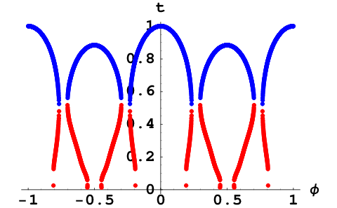
What is the correction to that arises from the finiteness of the radius? By taking into account this correction we arrive at the following equation obeyed by the critical temperature (see Appendix B.3 for the derivation):
| (20) | |||||
where we recall that , is the BCS constant , we have defined , which is related to the number of Cooper pairs, and the function is defined via the hypergeometric function AbramowitzStegun:
| (21) |
In Figs. 4 and 5 we show the flux dependence of the critical temperature for two particular ring radii. For the larger radius case, the value of at is essentially the same as that at and ; for the smaller radius case and for (i.e. all the pair states are occupied at and below Fermi level), the amplitude at is reduced, relative to that at and . Thus, as the radius becomes small we clearly see the emergence of the single-particle flux quantum period . Also worth noticing is the occurrence of a second solution (with lower value) for the critical temperature at sufficiently small radii, shown in Fig. 5. Compared to the higher solutions, for which our approximation of the equation (20), by keeping only the first two correction terms yields rather precise values, the evaluation of at these lower values of temperatures requires more terms (e.g. four or more) to be included in order to maintain the same accuracy.


For the case of large rings (i.e. ), to determine the leading corrections it is adequate to retain only the term and to set the correction to zero, when compared to values of order unity, in the second function. Thus, we arrive at the formula
| (22) |
The change in the reduced critical temperature is then approximately given by
| (23) |
where we have used the fact that . Again, the integer is to be chosen to minimize . We see that, in addition to the parabolic dependence on , there is a sinusoidal correction of period . This is the emergence of the single-particle flux dependence. We also note that this correction is not universal, in that it depends sensitively on the value of [and, moreover, the form of results from the simple quadratic single-particle spectrum]. It can happen that the correction due to the finiteness of the radius actually increases the critical temperature, i.e. when .
As we have argued using the results of Sarma Sarma and Maki and Tsuneto MakiTsuneto, the occurrence of multiple solutions in Eq. (15) for , for certain ranges of , leads to a change from a continuous to a discontinuous superconducting-to-normal phase transition. Even with the corrections to due to the finite-radius effect, as the radius of the ring decreases (to a value comparable to the coherence length), we observe that Eq. (20) still possesses multiple solutions for for certain ranges of ; see Fig. 5. This implies that somewhere in these ranges (of ) there exists a change from continuous (at larger radius) to discontinuous (at smaller radius) superconducting-to-normal transition. This is shown schematically in Fig. 6. If the radius is sufficiently large, the transition is always continuous. If the radius is sufficiently small, the the curve representing the discontinuous transition in one “dome” can intersect with that of the nearby dome (above the “void” region where no solution for of Eq. (20) exists). If this void region is large, the curve of the discontinuous transition can go to at certain value of without intersecting that from the nearby dome. However, calculations of alone cannot determine the precise location of the change from continuous to discontinuous; considerations of free energies are necessary to settle this issue.
III Disordered regime


How does disorder, in the form of potential scattering from fixed impurities, alter the physical picture that we have obtained so far? Does it affect the critical temperature? Does it change the order of the superconducting-to-normal transition? We now address these issues, assuming that the configuration of the impurities is sufficiently random that the tendency towards CDW formation is not enhanced.
III.1 Expansion of anomalous Green function; disorder average
For the most part, we shall consider impurities that produce scalar potential scattering; mutatis mutandis, the effects of exchange and spin-orbit scattering can be straightforwardly included. To begin with, we include potential scattering via the term in the Gor’kov equations Gorkov, which now read (here we restore the constants and )
| (24a) | |||
| (24b) | |||
where represents the potential from static impurities, i.e.,
| (25) |
and indicates the spatial location of impurity.
Following Gor’kov Gorkov, we introduce a Green function that satisfies
| (26) |
We can then express exactly in terms of and as
| (27) |
Because we are only concerned with solving for , near the transition, it is sufficient to keep G to zeroth order in and replace in Eq. (27) by ; thus we have
| (28) |
We now consider the self-consistency equation (2), and average over the quenched disorder associated with the locations of the impurities:
| (29) |
where indicates disorder averaging. We note that, as explained by Gor’kov Gorkov, the Green function oscillates on a much smaller length scale than and, hence, the disorder average of can be factorized. For convenience, we use to denote the disorder average of , i.e., , the translational invariance of which is restored, viz.,
| (30) |
To calculate the disorder average of the product of two Green functions, we introduce the kernel Gorkov, defined via
| (31) |
If we retain only the ladder diagrams (i.e. ignoring the crossed diagrams AG59), we arrive at the result
| (32) |
where we have simplified the notation by dropping the subscript on and moving from an argument to a subscript, and is the impurity concentration. Assuming that the order parameter retains the form , the self-consistency equation can be reduced to
| (33) |


III.2 Critical temperature
We leave the detailed calculation of the kernel to Appendix B.4 and simply quote here the resulting equation (B.4.2) for the critical temperature in the disordered regime, i.e. :
| (34) | |||||
where is the elastic mean free path, is the elastic scattering time, we recall that , and
| (35) |
We remark that the argument in the second digamma function in Eq. (34) is real, in contrast with the clean case, for which it is complex; see Eq. (11). A consequence of this is that there is no longer a doublet of solutions for . Moreover, the resulting single solution is consistent with the assumption that the order parameter becomes vanishingly small as the temperature approaches its critical value from the superconducting side. Therefore, the transition to the superconducting state is continuous.
To explore the consequences of Eq. (34), we first examine the large-radius (i.e. bulk) limit, and show that we recover the de Gennes results for the case of rings. We then proceed to compare how the finiteness of the radius affects the oscillations of .
III.2.1 Large-radius limit
Ignoring correction due to the finiteness of the radius, we obtain the following equation for of the bulk superconductor, i.e.,
| (36) |
as we should. This is in agreement with the results of de Gennes’ deGennes for rings and those obtained by Lopatin et al. LopatinShahVinokur for hollow cylinders. To see that the de Gennes results are recovered, we note that the critical value of , beyond which no superconducting solution for any exists, is given by footnote. For a fixed radius, this defines the critical flux , which defines the boundary between normal and superconducting states. We then determine that the critical flux satisfies
| (37) |
which gives the critical flux for a given radius, or vice versa, via
| (38) |
When the flux dependence of the critical temperature is weak, as in the large-radius limit, is close to unity and , so one can expand the logarithm in and the second digamma function around in Eq. (36) to obtain
| (39) |
As we did for Eq. (19) in the clean limit, we can express this equation as
| (40) |
where is the temperature-dependent Ginzburg-Landau coherence length in the dirty limit. Thus, we recover the de Gennes results deGennes, but via a microscopic calculation. We note that, strictly speaking, the Ginzburg-Landau approach is only valid near (see also discussion at the end of Sec. II.2.1).
III.2.2 Finite-radius regime
Strictly speaking, the de Gennes results (40) are only valid in the large-radius limit, as is clearly seen from our microscopic derivation. In the regime in which the radius of the ring is comparable to the zero-temperature coherence length or the Cooper-pair size, we should take into account the effect of finite radius and use Eq. (34) instead of Eq. (36). In addition to the lengthscale defined by the Cooper-pair size , the behavior of also depends on another length scale, viz., the mean-free path . The correction terms (i.e. the terms in the summation) in Eq. (34) decay exponentially with , so that the series converges rather rapidly, even for or slightly smaller. In Fig. 7 we contrast the predictions of in the large-radius limit, Eq. (36), to those that include the finiteness corrections, Eq. (34), for a small radius (). Figure 7 also shows that the oscillation has a component of period , in addition to the usual Little-Parks component of period . In Fig. 8 we plot the critical temperature vs. radius for various flux values. We see that the deviation from the bulk result is mroe significant near , whereas the bulk result shows almost no deviation in the range .
The deviation of the critical temperature of small-radius rings from that of large-radius rings is, however, not universal, as it depends on both the magnitude and sign of . We have seen that when the sign of is positive, the corrections from the finiteness of the radius can cause a reduction in the critical temperature near the flux value , compared to the bulk case. This corresponds to the case in which, at zero flux, all the electrons are paired up. However, when the sign of the cosine is negative, the critical temperature at can actually exceed its value at zero flux; this corresponds to the case in which, at , all electrons are paired up, thus the system is more stable there than at . If the cosine term should happen to vanish accidentally, the oscillation at period would disappear.
When the radius is not small the change in , relative to , is small, and we therefore need only retain terms in Eq. (34) to order and also may replace on the r.h.s. by 1, as we did to obtain Eq. (39). Thus we obtain
| (41) |
Hence, an oscillation of period is clearly seen to emerge, and whether the critical temperature reduces or increases (e.g. at ), compared to the bulk Little-Parks value, is seen to depend on the sign of the cosine term. For the case where all electrons are paired up at zero flux, the critical temperature is lower at than at .
IV Concluding remarks
We have considered the oscillations in the critical temperature of a superconducting ring of finite radius in the presence of a threading magnetic flux. We have found that, as the radius of the ring is (parametrically) reduced, an oscillation in the critical temperature of period of emerges, in addition to the usual Little-Parks dependence (the period of which is ). Our results provide corrections, due to the finiteness of the ring radius, to the results that de Gennes obtained for a flux-threaded ring deGennes. We have argued that in the clean limit there is a superconductor-normal transition, as the ring radius becomes sufficiently small at nonzero flux, and that the transition can be either continuous or discontinuous, depending on the radius and/or flux. In the disordered regime, we have argued that the transition is rendered continuous, which results in a quantum critical point tuned by flux and radius.
One may wonder how the system behaves as it goes from clean to dirty limit. At which point does the existence of multiple solutions in the critical temperature disappear? By analyzing Eq. (88), we obtain that, ignoring the finiteness corrections, double solutions disappear when the disorder is such that .
One question we should also address is the thickness of the ring cross-section. It causes an orbital pair-breaking effect. For the purpose of estimating this we can use the result from a wire with same thickness in a field perpendicular to the wire axis (for the calculation, see, e.g. Ref.Tinkham). The fractional decrease of critical temperature, when it is small, can be estimated to be (not including the oscillation by flux)
| (42) |
which causes a quadratic decrease in the critical temperature on top of the oscillations discussed in the present paper. If we take the same values shown in Fig. 7, i.e., , for the decrease is about at and about at . The largest decrease in the critical temperature shown in Fig. 7 is about , and the component is not swamped by the pair-breaking effect and can still be observed.
Although we have obtained the emergence of the oscillation and its amplitude by the microscopic calculations, the physics behind these effects can be illustrated via heuristic arguments associated with the corresponding Cooper problem on a ring, together with a path-integral based instanton tunneling approach. We briefly discuss these points in Appendix C.
The non-universal factor determines whether the finiteness of the ring radius leads to a decrease or an increase in the critical temperature near flux . Although this factor is model dependent (i.e. dependent on the form of the single-particle spectrum), for the quadratic spectrum we consider here, roughly counts the number of electrons divided by four, as there are two spin species and positive and negative (angular) momenta. If we restrict ourselves to the case in which all electrons are paired then , because for two electrons can still occupy the state. When all the levels at and below are filled at zero flux, . When there is one pair fewer or more (or equivalently, when all pairs are occupied at ), . This seems to result in an even-odd effect, not from the number of electrons RalphBlackTinkham95 but from the number of Cooper pairs. However, whether this even-odd effect holds in general requires further investigation.
Notes added in proofs. 1. We would like to point out that the issue of flux-dependent supercurrents for s-wave rings was also studied by Zhu and Wang in Ref. 28. In addition to Refs. Dwave; JuricicHerbutTesanovic07; Barash07, there is a more recent work on the same issue in d-wave superconductors in Ref. 29.
2. Throughout our paper, we have essentially assumed that the switching of pairing configuration (see Fig. 2) occurs at flux values being an odd integer multiple of near superconducting-normal transition temperatures. This is consistent with our numerical results that by allowing the switching to be varied, the largest possible critical temperature is obtained when the above assumption is obeyed. In a very recent paper by Vakaryuk in Ref. 30, the author concludes that the switching can be flux dependent at zero temperature. If the two results are to be consistent, we are led to the conclusion that the switching is temperature dependent. This requires further investigation.
Acknowledgments. The authors acknowledge informative discussions with David Pekker and Frank Wilhelm, and are especially grateful to Gianluigi Catelani for his critical reading of this paper. This work was supported by DOE Grant No. DEFG02-91ER45439 through the Federick Seitz Material Research Laboratory at the University of Illinois. TCW acknowledges the financial support from IQC, NSERC, and ORF, as well as the hospitality of Perimeter Institute, where part of this work was done. We would also like to acknowledge V. Vakaryuk and A. J. Leggett for communicating the results of Ref. 30.
Appendix A Averaged Gor’kov equations over radial direction
Consider a ring on a plane with inner and outer radii and , respectively. Assume that the thickness is much smaller than the mean radius and the zero-temperature coherence length . We reduce the two dimensional Gor’kov equations into effective one-dimensional equations by defining the averaged Green function,
| (43) |
and similarly for . Under this averaging, the two-dimensional delta function becomes one-dimensional,
| (44) |
In the Laplacian operator, there is a term . When performing the above average, we get for this term
| (45) |
which, under the condition of no current flowing radially through the ring boundary, gives zero identically. Similarly, if we regard the anomalous Green function as playing the role of the Ginzburg-Landau order parameter in the theory of superconductivity, no-flow of supercurrent radially gives the average to be zero for . Furthermore, under the limit that the average of the product of two functions can be approximated by the product of two averaged functions, we obtain a set of reduced one-dimensional Gor’kov equations, with the coordinate variables being azimuthal angles and and the radii being set to the fixed value of the average radius. After appropriately renormalizing the Green functions by the inverse of the average radius (thus making the dimension consistent), we arrive at Eqs. (3). We remark that even if the ring has the geometry of a torus, the same averaged 1D equations will result provided that the cross-section is relatively small, compared with the ring area and the coherence length.
Appendix B Critical temperature equations: supplementary details
In this appendix, we supplement the details leading to the critical temperature equations in both clean limit and the disordered regime.
B.1 Clean limit
Continuing from Eq. (9), we make a shift in : , under which the integral becomes
| (46) |
where . The integral over can be performed using contour integration. For example, for and , we can close the contour in the upper plane and evaluate the residues at and . We end up with (noting the cancellation of the factor )
| (47) | |||
| (48) |
Including the contributions from the three other cases, we arrive at the self-consistency equation:
| (50) | |||||
where we have put the Debye frequency as the upper cutoff in the Matsubara sum. This equation can be re-written as
| (51) | |||||
| (52) |
Furthermore, for typical temperatures we have . The second term causes the contribution of the terms to be exponentially small for large , i.e. there is a factor
| (53) |
B.2 Large-radius limit
For sufficiently large , we can ignore the correction terms, in which case we have
| (54) |
The third term in the denominator is usually much larger than the second term, as the chemical potential is much larger than the level spacing , i.e., . For typical values of and , we have . Hence, we have
| (55) | |||||
| (56) |
The solution for to this equation gives the critical temperature . Denoting by the critical temperature in the absence of flux (so that ), we have the corresponding equation
| (57) |
Taking the difference of equations (55) and (57), we have
| (58) |
If we extend both upper limits to infinity, we should compensate by the difference (assuming ), i.e.,
| (59) |
Therefore, we arrive at
| (60) |
In terms of the digamma function in Eq. (12), we have an implicit formula for :
| (61) |
Using the quantities , , and , and defining , we can re-write Eq. (61) as
| (62) |
B.3 Finiteness correction
What is the correction to due to the finiteness of the radius? To address this question we need to take into account the corrections to Eq. (52). If we take and , the self-consistency equation (52) can be approximated as
| (63) | |||||
| (64) |
Taking the difference between this equation and the version corresponding to , and using the trick for converting the cutoff at the Debye frequency in a logarithm (see Eqs. (59)-(61), we arrive at
| (65) | |||
| (66) |
where the dependence of on r.h.s. is suppressed. We have extended the upper limit of the sum over to infinity for the exponentially decaying terms (which introduces a negligible small error), and we have used the formula
| (67) |
where is the hypergeometric function .
B.4 Disordered regime
In this subsection, we calculate and and obtain the r.h.s. of the self-consistency equation (32). For simplicity, we assume that the potential is short-ranged, so that its Fourier transform can be treated as a constant, essentially independent of momentum transfer .
The one-particle self-energy can be obtained from summing one-particle-irreducible diagrams (and ignoring the crossed diagrams), and thus we obtain
| (68) |
the real part of the self-energy has been ignored and we shall call the frequency-dependent scattering time. Under the condition that the Debye frequency is much smaller than the chemical potential, i.e. , and hence for the range of ’s that are relevant to superconductivity (i.e. ), we obtain
| (69) |
where
| (70) |
This form for is an approximant because it is calculated with rather than . To improve the approximation we then use the exact disordered Green function to calculate the same self-energy diagrams again (see, e.g. Ref. AGD), thus obtaining a self-consistency condition for (that can be solved iteratively):
| (71) |
As the terms are exponentially small, we can approximate on the right-hand side by to arrive at
| (72) |
Returning to the kernel , we re-write Eq. (32), following Gor’kov Gorkov, as
| (73) |
where we have conveniently dropped the sign in , and
| (74) |
and the argument in reflects the conservation of total (azimuthal) momentum of the two incoming (and outgoing) electrons in the ladder diagrams after disorder averaging. For the purpose of evaluating self-consistency equation (33), our goal is to obtain for . By eliminating from Eqs. (73) and (74) by we have an equation for :
| (75) |
which gives
| (76) |
where
| (77) |
The self-consistency equation (33) then becomes
| (78) |
where we have used Eq. (70) in the second equality. As with the evaluation of Eq. (46) in the clean limit (see Appendix B), we obtain as
| (79) | |||||
where , , and is a shorthand for .
To illustrate the corrections arising from the finiteness of the radius, we re-write as
| (80) |
where and are
| (81a) | |||||
| (81b) | |||||
As the correction to is exponentially small [see Eq. (72)], in the exponentials can be approximated by
| (82) |
On the other hand, for not in the exponentials we shall approximate it by retaining the leading correction [see Eqs. (72) and (81a)] via
| (83) |
The quotient then becomes
| (84) |
We remark that from this equation one can obtain the equation for the critical temperature for arbitrary mean-free path .
B.4.1 Large-radius limit and arbitrary disorder
To illustrate the remark made above, we consider large-radius limit in which we ignore corrections due to the finite radius. In this limit Eq. (84) becomes
| (85) |
Substituting this into Eq. (78) we have
| (86) |
In the clean limit , we see that this reduces to Eq. (56), which we obtained in the absence of disorder. But here is arbitrary. Subtracting Eq. (86) from the corresponding equation at (i.e. ) and using the trick to get logarithm of the ratio of the critical temperatures as we did in Eqs. (59)-(61), we have
| (87) |
By making the partial fractions of the first term in the summation and by using the definition of the digamma function (12), we arrive at
| (88) | |||||
where, for convenience, we have defined and . This is the equation for the critical temperature at arbitrary disorder for large radii of rings.
B.4.2 Finite-radius corrections and strong disordered regime
Now we return to the corrections due to the finiteness of the radius. In the strong disordered limit (i.e. ), Eq. (84) becomes
| (89) |
This is further approximated, using Eq. (83) as
| (90) |
where we have used Eq. (83). The first term on the r.h.s. represents the bulk term and is the Little-Parks term in the dirty limit. The second term takes into account the finite radius, and contains flux dependence in period . The equation for the critical temperature will then contain the digamma function and hypergeometric function with real arguments, in contrast with the clean limit. This makes the transition to normal state continuous, as the solution for the critical temperature is unique and the assumption of vanishing order parameter used in the linearized self-consistency condition is valid. Therefore, there can be quantum phase transitions tuned by flux and/or radius.
As in the strong-disorder limit, the ratio becomes (by ignoring the term)
| (91) |
From this we can obtain an equation for the critical temperature in the presence of flux , as we have done in the clean limit (see Appendix B.3). By inserting Eq. (91) into the self-consistency equation (78) we obtain
| (92) |
Subtracting from this the corresponding equation, i.e.,
| (93) |
we obtain the following implicit equation for the critical temperature:
| (94) | |||||
where we have used the fact that when or higher, , the sum of the series being approximated is a logarithm, and we have extended the upper limit of for the correction terms to infinity. By using formula (67) for the hypergeometric function, we finally arrive at
| (95) |
where we recall that . If we use , , and (with ), we have
| (96) |
We can re-write this equation using the relations , and , and thus arrive at
| (97) |
B.4.3 Finite-radius and arbitrary disorder
It is also possible to include corrections from the finiteness of the radius, and derive the equation for the critical temperature, as we did in the previous section. The results will contain the r.h.s. of Eq. (88) as the zeroth order, as well as corrections due to the finiteness of the radius in terms of hypergeometric functions. However, the formulas are too cumbersome and we do not list them here.
Appendix C Heuristic argument to the emergence of period oscillations
C.1 Cooper problem on a ring
Let us consider Cooper’s problem on a ring with a flux threading through it. The orbital wavefunction can be written in the same form as in Eq. (4). Assuming that , and that the electron-electron interaction is factorizable, i.e. , we can write down the time-independent Schrödinger equation in terms of the wavefunction amplitude as
| (98) |
where
| (99) |
and hence we arrive at
| (100) |
The integer has to be chosen to minimize the ground state energy. Thus, we see that the solution is periodic in with period 1 (or in with period , namely the single particle flux quantum) and that the Little-Parks period is exact only in the large- limit, in which case the summation over can be replaced by an integral and hence the period of is . This illustrates the role of the single particle oscillation. However, the amplitudes of the single-particle and Little-Parks oscillations have to be evaluated within a microscopic theory, as has been done in the main text.
C.2 Flux oscillation: an instanton approach
The instanton picture provides us another, heuristic, view of the emergence of -period oscillations. The argument presented here is intended just to give some intuition. We refer to Rajaraman Rajaraman for a pedagogical review of instanton techniques. A single instanton tunneling from through a potential to (which is identified as ) on a circle gives an amplitude
| (101) |
where is the classical Euclidean action (in the absence of any flux threading through the circle), is a Jacobian factor, is a constant independent of as , and is the harmonic oscillator frequency near the bottom of the trapping potential. Now, if there is a flux threading the ring, the amplitude will also acquire an additional phase factor , where and , if the particle carries charge . For a charge particle, the phase factor would be .
We consider a ring size that is large enough that the electrons in a Cooper pair generally traverse the ring together, and rarely split so as to wind separately around the ring. The ground state energy will give a qualitative estimate of the critical temperature of the associated superconductor. The total contribution of the amplitude for the instanton associated with the Cooper pair is then
| (102) |
which gives
| (103) |
This gives a ground state energy of , which reveals the period , the Little-Parks period in critical temperature. The fact that this gives a dependence on flux being sinusoidal rather than quadratic results from the lack of accounting of the other many-body electrons and the existence of a condensate.
Now, occassionally (in the sense of contributing Feynman paths) the electrons in a Cooper pair separate and circumnavigate the ring (relative to one another) before re-associating. The contribution of such processes to the ground-state energy can be estimated via the instantons and anti-instantons of such events associated with them. A single instanton involving one electron going from to has the amplitude
| (104) |
where the subscript indicates a single electron rather than a Cooper pair, and the additional minus sign comes from the exchange of the two electrons. Summing all the instanton and anti-instanton processes, we arrive at the contribution to the ground-state energy from the two electrons
| (105) |
which results in the emergence of an contribution to the period of oscillation to critical temperature. We remark that it is owing to the separation of the lengthscales and hence time scales that we can separate the Cooper-pair and single-electron contributions. The amplitudes of the two oscillations are related to the respective actions, and for large radius, the amplitude corresponding to single-particle oscillation is expected to be small, due to the binding resulting from the attractive interparticle interaction.
References
- (1) W. A. Little and R. D. Parks, Phys. Rev. Lett. 9, 9 (1962).
- (2) M. Tinkham, Introduction to Superconductivity, McGraw-Hill (1996), p.128-p.130.
- (3) See, e.g., J. R. Schrieffer, Theory of Superconductivity, Perseus Books (1983), Chapter 8, p.240-p.244.
- (4) Y. Liu, Yu. Zadorozhny, M. M. Rosario, B. Y. Rock, P. T. Carrigan, and H. Wang, Science 294, 2332 (2001). H. Wang, M. M. Rosario, N. A. Kurz, B.Y. Rock, M. Tian, P. T. Carrigan, and Y. Liu, Phys. Rev. Lett. 95, 197003 (2005).
- (5) P. G. de Gennes, C. R. Acad. Sci. Ser. II 292, 279 (1981).
- (6) R. A. Webb, S. Washburn, C. P. Umbach, and R. B. Laibowitz, Phys. Rev. Lett. 54, 2696 (1985).
- (7) H. Bluhm, N. C. Koshnick, M. E. Huber, and K. A. Moler, Phys. Rev. Lett. 97, 237002 (2006).
- (8) N. C. Koshnick, H. Bluhm, M. E. Huber, and K. A. Moler, Science 318, 1440 (2007).
- (9) K. Czajka, M. M. Maśka, M. Mierzejewski, and Z. Śledź, Phys. Rev. B 72, 035320 (2005).
- (10) F. Loder, A.P. Kampf, T. Kopp, J. Mannhart, C. W. Schneider, Yu. S. Barash, Nature Phys. 4, 112 (2008).
- (11) V. Juricic, I. F. Herbut, and Z. Tesanovic, e-print arXiv:0711.3790 (2007).
- (12) Yu. S. Barash, e-print arXiv:0711.4338 (2007).
- (13) J. Bardeen, L. N. Cooper, and J. R. Schrieffer, Phys. Rev. 106, 162 (1957).
- (14) L. P. Gor’kov, Soviet Physics JETP 9, 1364 (1959); ibid. 10, 998 (1960).
- (15) In C.G.S unit, the single-particle flux quantum is . We shall set and . Even though in this unit the flux quantum becomes , we shall refer to it by instead.
- (16) See, e.g., A. L. Fetter and J. D. Walecka, Quantum Theory of Many-Particle Systems (McGraw-Hill, New York, 1971).
- (17) Although we take the ring to be of infinitesimally thin width, for small but finite width compared to the radius and the coherence length, this set of equations can be obtained by averaging over the radial direction and ignoring the fluctuations; see Appendix A. In our discussions we require that the mean average level spacing in the transverse direction is much greater than the superconducting gap , so that only the lowest level in the transverse direction is occupied. This leads to the condition that , where is the Cooper-pair size .
- (18) M. Abramowitz and I. A. Stegun, Handbook of Mathematical Functions (National Bureau of Standards, 1972), p.259 and p.556.
- (19) G. Sarma, J. Phys. Chem. Solids, 24, 1029 (1963).
- (20) K. Maki and T. Tsuneto, Prog. of Theor. Phys. 31, 945 (1964).
- (21) Note that here we assume the equilibrium normal state does not possess a persistent current. Ignoring the finiteness correction, the transition to normal follows the curve ABD in Fig. 3. If the normal state does possess a persistent current, the transition from superconducting to normal will follow the curve ABE instead. The inclusion of the finiteness correction only modifies the detail locations of these curves.
- (22) L. P. Gor’kov and A. A. Abrikosov, Soviet Physics JETP 8, 1090 (1959).
- (23) Sec. 39.2, Chapter 7, in A. A. Abrikosov, L. P. Gor’kov, and I. E. Dzyaloshinski, Methods of Quantum Field Theory in Statistical Physics (Dover, 1975).
- (24) A. V. Lopatin, N. Shah, and V. M. Vinokur, Phys. Rev. Lett. 94, 037003 (2005).
- (25) This can be seen from the fact that the function , is greater than zero for when , whereas it crosses from negative values to positive at a certain value of when .
- (26) D. C. Ralph, C. T. Black, and M. Tinkham, Phys. Rev. Lett. 74, 3241 (1995)
- (27) R. Rajaraman, Solitons and Instantons, Chapter 10 (North Holland, 1987).
- (28) J.-X. Zhu and Z. D. Wang, Phys. Rev. B 50, 7207 (R) (1994).
- (29) J.-X. Zhu, eprint arXiv:0806.1084.
- (30) V. Vakaryuk, eprint arXiv:0805.2626.