Forming galaxies with MOND
Abstract
Beginning with a simple model for the growth of structure, I consider the dissipationless evolution of a MOND-dominated region in an expanding Universe by means of a spherically symmetric N-body code. I demonstrate that the final virialized objects resemble elliptical galaxies with well-defined relationships between the mass, radius, and velocity dispersion. These calculations suggest that, in the context of MOND, massive elliptical galaxies may be formed early () as a result of monolithic dissipationless collapse. Then I reconsider the classic argument that a galaxy of stars results from cooling and fragmentation of a gas cloud on a time scale shorter than that of dynamical collapse. Qualitatively, the results are similar to that of the traditional picture; moreover, the existence, in MOND, of a density-temperature relation for virialized, near isothermal objects as well as a mass-temperature relation implies that there is a definite limit to the mass of a gas cloud where this condition can be met– an upper limit corresponding to that of presently observed massive galaxies.
1 Introduction
Here I reconsider the problem of galaxy formation, dissipationless and dissipational, in the context of modified Newtonian dynamics, or MOND (Milgrom 1983). With Newtonian gravity, dissipational processes do not appear to be necessary to explain the basic structural properties of elliptical galaxies. For example, van Albada (1982) demonstrated that the observed surface brightness profile of elliptical galaxies, the law (de Vaucoleurs 1948), develops naturally in Newtonian N-body simulations of the collapse of bound systems with initially inhomogeneous density distributions. On the other hand, dissipation does seem to be necessary to explain the typical densities of baryonic matter in both disk and elliptical galaxies (Binney 1977); pure gravitational collapse in an expanding Universe produces insufficient concentration of visible matter. Moreover, cooling and fragmentation are certainly necessary for the formation of stars which are the principal component of galaxies. Thus, the formation of galaxies could, in some sense, be viewed as dissipationless if cooling of a primordial gas cloud and fragmentation down to the level of stellar mass objects occurs on a time scale short compared to that of dynamical collapse. This is a point first made by Hoyle (1953) to explain the mass scale of galaxies, and developed further by a number of authors (Silk 1977, Binney 1977, Rees & Ostriker 1977, White & Rees 1978). The argument involving these two competing timescales has become an essential ingredient of the standard cosmology in which the matter budget of the Universe is dominated by a hypothetical pressureless, collisionless fluid, cold dark matter, or CDM (White & Rees 1978, Blumenthal et al. 1984).
In the context of the MOND paradigm, galaxy formation must occur without the assistance of CDM. Moreover, recent numerical work has indicated that dissipationless merging of galaxies proceeds much more slowly with MOND than when luminous galaxies are assumed to be surrounded by massive dark halos (Nipoti, Londrillo & Ciotti 2007b); therefore, mergers would probably play a less important role in galaxy formation, particularly the formation of ellipticals, than in the current conventional picture. But the primary roadblock to the consideration of galaxy formation with MOND is that there is not yet a generally accepted or standard cosmological context for structure formation, even though relativistic extensions have been described in the literature (e.g., Bekenstein 2004, Sanders 2005, Zlosnik, Ferreira & Starkman 2006). Therefore, I begin with the simple assumptions that MOND only applies to peculiar accelerations in an expanding Universe and that the acceleration constant, , does not evolve with cosmic time.
Such assumptions would appear to be consistent with the current relativistic versions of MOND, where the non-Newtonian force is mediated by a long-range scalar field with non-standard Lagrangian: there is no MOND in the absence of density variations. Moreover, these assumptions underly the heuristic models of structure formation in a MONDian universe considered previously by myself (Sanders 2001) and by Nusser (2002). In particular, Nusser noted that small fluctuations grow rapidly (), and that this leads to a unacceptably clumpy Universe at the present epoch– essentially independent of the initial amplitude of fluctuations. I postpone consideration of this problem to a later discussion on taming the growth of large-scale structure formation and assume here that galaxy scale fluctuations in a baryonic Universe grow by the application of the MOND formula to peculiar accelerations. If so, then it is easily demonstrated that galaxy mass objects re-collapse early () and that spherically symmetric dissipationless collapse leads to final virialized objects having roughly the properties of observed elliptical galaxies. In particular, both the magnitude and form of the observed surface density distribution –the de Vaucoleurs law– and the velocity dispersion-baryonic mass relation– the Faber-Jackson law (Faber & Jackson 1976)– are reproduced for bound objects with masses ranging up to .
All of this, however, begs the question of why galaxies, as self-gravitating ensembles of stars, have an upper mass limit to their baryonic content of about . More massive self-gravitating objects exist, but they are bound groups or clusters of galaxies rather than single entities consisting of stars. To address this question we must again consider the processes of radiative cooling and fragmentation on a time scale short compared to that of gravitational collapse. In this respect, there is a great advantage afforded by modified dynamics: the presence of an additional physical constant with units of acceleration ( cm/s2) in the structure equation strongly constrains the properties of any self-gravitating object as we see in this and previous dissipationless collapse calculations (Nipoti, Londrillo & Ciotti 2007a). Such an object with a velocity dispersion of a few hundred km/s will have a mass of M⊙ as well as a characteristic size and density. In other words, there is less arbitrariness in specifying initial properties of a pre-galactic cloud.
In the context of MOND the virial mass, the dynamical timescale, and the characteristic density of a self-gravitating isothermal cloud depend only upon velocity dispersion. This redefines the curve, in the temperature-density plane, describing the condition that dynamical and cooling timescales are equal. As in the standard model, this curve neatly separates those objects where dissipation has led to the formation of stars (galaxies) from those where it has not (groups and clusters). Moreover, the presence of a density-temperature relation for self-gravitating isothermal clouds leads to definite upper limit to the mass of objects in which the cooling time is less than the dynamical time– again a characteristic mass of about M⊙. Therefore, we see that many of the successes of the standard model for galaxy formation carry over to MOND– in particular the existence of an upper limit to systems consisting of stars. Moreover, the location of near isothermal systems in the temperature-density plane– systems ranging from globular clusters to clusters of galaxies– plane becomes understandable in terms of MOND.
In the following section I review the heuristic model for the initial growth of galaxy scale fluctuations in an expanding Universe. In section 3 I numerically follow the dissipationless evolution of galaxy-scale spherical regions which collapse out of the Hubble flow. Even though dissipationless, these calculations demonstrate the scaling relations which primordial gas clouds may obey. In section 4 I apply these relations to reconsider the old argument on collapse and fragmentation in the context of MOND, and in the final section I compare MOND with the standard model and summarise.
2 The growth of small fluctuations in a MONDian Universe
MOND in its original form (Milgrom 1983) is described by the relation between the true gravitational acceleration, , and the Newtonian gravitational acceleration, –
where is the fundamental acceleration parameter ( cm/s2) and is the function which interpolates between the Newtonian regime (, ) and the MOND regime (, ). MOND, as a modification of Newtonian gravity, may also be expressed by the modified field equation of Bekenstein & Milgrom (1984):
This formulation is conservative but difficult to solve for arbitrary mass distributions; in the case of spherical symmetry it reduces to the simple expression above (eq. 1) where is determined by the usual Poisson equation.
Early efforts to describe a MONDian cosmology in the absence of a relativistic theory applied the simple MOND equation (eq. 1) to an expanding spherical region analogously to the Newtonian derivation of the Friedmann equation (Felten 1984). There it was immediately realized that the evolution depended upon the physical size of the region (it was not possible to define a dimensionless scale factor) and that any expanding region would eventually re-collapse regardless of its initial density and expansion velocity. However, at early epochs, the region within which the Hubble deceleration is less than , is much smaller than the horizon scale; therefore, if is independent of cosmic time, it may be possible that the Universe as a whole is Friedmannian while increasingly larger sub-regions become MONDian and re-collapse (Sanders 1998). Although this would lead naturally to a scenario of hierarchal structure formation, it is not possible to identify the centres of re-collapse; i.e., primordial density fluctuations play no role.
A more plausible scenario would be one in which the MOND formula is applied to the peculiar accelerations developing from density fluctuations rather than to the Hubble expansion as a whole. This was the central idea behind heuristic models for structure formation (Sanders 2001, Nusser 2002) and for the early collapse of low-mass gas clouds [Stachniewicz & Kutshera 2005]. This assumption is consistent with, but not a necessary consequence of, current relativistic extensions of MOND (for example, TeVeS, Bekenstein 2004). Its validity depends upon the form of the free function of the theory (effectively the MOND interpolating function) in the cosmological regime where the cosmic time derivative of the scalar field dominates the scalar field invariant. But since the free function does not follow from any more fundamental considerations, assumptions about its form, at present, are no less ad hoc than applying the MOND prescription directly to peculiar accelerations.
With the additional ansatz that the MOND acceleration parameter is does not vary with cosmological time (also not necessarily true in relativistic extensions such as the biscalar variant of TeVeS, Sanders 2005), the equation for the growth of small fluctuations (() becomes:
Here is the dimensionless scale factor in terms of the present scale factor (), time is in units of the Hubble time (), is the co-moving scale of the perturbation, and is the peculiar gravitational acceleration related to the Newtonian peculiar acceleration
by the MOND formula (eq. 1). Here I have assumed that fluctuations grow primarily during the period when non-relativistic matter with density parameter dominates the mass-energy budget of the Universe. Below I will assume, consistent with MOND, that this matter is essentially baryonic.
In the high acceleration limit () we recover the usual linear Newtonian expression for the growth of small fluctuations in an expanding medium (). However, when , then the MOND limit applies:
where is the Hubble radius, , and the MOND acceleration parameter is written as with . In this case, the equation for the growth of small fluctuations becomes non-linear () and dependent upon the co-moving or mass scale.
In the MOND limit a simple power law solution to this equation exists in the matter dominated regime; i.e., with . In other words, unlike the Newtonian case where , in the MOND regime (Nusser 2002). In terms of the scale factor, the solution is
In fact, as may occur in non-linear problems, this solution is an attractor on a space of solutions; MOND drives structure growth toward quite independently of the initial conditions.

This is shown in Fig. 1, where is plotted as a function of scale factor. The cosmological background here is of the usual Friedmann form for a Universe without dark matter () but with the standard radiation content and zero spatial curvature, i.e., . Note that here I do not consider the possible presence of 2 eV neutrinos; this would change details– on the scale of galaxies, adding an additional contribution to Hubble expansion– but not the essence of the argument. In eq. 1 I have taken the form of to be that advocated by Zhao & Famaey (2006), i.e., . The heavy solid curve is the pure MOND power law solution (eq. 6) for a co-moving scale of 1.56 Mpc corresponding to a mass of , and the lighter solid curves are numerical solutions of eq. 3 with various initial values for at the epoch of matter decoupling (). We see that the numerical solutions rapidly converge to the power law solution.
It is also evident that the fluctuations grow to unity on a at relatively early epoch:
corresponding to a redshift of for the galaxy scale fluctuation. In this scenario we would expect massive galaxies to form early ().
Given that the power spectrum of fluctuations is related to the amplitude as this gives a final power spectrum of as noted by Nusser (2002). However, also as noted by Nusser, eq. 6 would certainly imply that the amplitude of fluctuations on large scale is far too large to be consistent with observations. Cosmology can intervene to tame the growth of larger scale structure; essentially, vacuum energy (or curvature) moderates the growth when it begins to dominate the cosmic expansion, but this will be considered in a later paper. For now, we assume that eq. 6 applies to galaxy scale fluctuations. Of course, the equation is only valid when ; thus below we consider the dissipationless evolution of collapsing spheres with MOND; i.e., only (modified) gravity affects the evolution. The underlying implicit assumption is that the baryonic fluid, presumably a gas cloud at the beginning of re-collapse, rapidly cools, fragments and forms stars during the initial collapse. The condition for this to occur will be considered in Section 4.
3 The expansion and re-collapse of MOND dominated fluctuations
Fully three-dimensional dissipationless collapse calculations have recently been carried out by Nipoti et al. (2007a). Starting with an inflated Plummer sphere (zero initial kinetic energy) they follow the collapse and formation of virialized objects with varying central concentration, ranging from deep MOND to Newtonian. Here I use a spherically symmetric N-body code of the form originally developed by Hénon (1964) in order to follow the evolution of an initially expanding over-dense spherical region beyond . Although the calculations of Nipoti et al. would provide more realistic models of actual galaxies, the goal here is to consider the general properties of objects which might actually condense out of the Hubble flow.
The radial motion of spherical shell at radius is determined by numerically solving the equation of motion:
where the gravitational force at the shell, , is given by two parts: where is the usual Hubble deceleration and , as above, is the peculiar deceleration resulting from the over-density and given by the MOND formula (eq.. 1), again with the Zhao-Famaey interpolating function. Whenever the peculiar acceleration exceeds the Hubble acceleration by a factor of two, I assume that the region is decoupled from the Hubble flow and then follow its evolution as an isolated object. The final term in eq. 8 is the centrifugal acceleration with being the specific angular momentum of the shell; i.e., where is the tangential velocity of particles comprising that shell. Note that there is no systematic rotation; of particles in a shell is assumed to be distributed uniformly in all tangential directions. Again, because of the perfect spherical symmetry the solution of eq. 1 is equivalent to solving the Bekenstein-Milgrom modified Poisson equation.
The sphere is initially homogeneous and partaking in the uniform Hubble expansion perturbed by its peculiar velocity. An initial over-density of is simulated by taking the sphere to be initially slightly smaller () than it would be in a uniform Universe. The initial conditions for the expanding sphere then are taken from the numerical solution for described above (as in Fig. 1) in the case where the fluctuation amplitude at decoupling is . For the sphere with mass , when we find in units of the Hubble time, corresponding to which yields an initial radius of 15.1 kpc and an expansion velocity of 254 km/s (this is all for the adopted cosmological model). The expansion is taken to be linear () out to the maximum radius. The initial tangential velocity on all shells is assumed to be 20-30 km/s in order to prevent a collapse which is too violent (the results are qualitatively insensitive to the actual value of ). With MOND, the over-dense sphere will inevitably re-collapse after reaching a maximum radius about 3 times larger than the initial radius. The re-collapse occurs after a time interval comparable to the age of the Universe at the epoch when the sphere decouples from the Hubble flow. Of course, the assumptions of uniformity and spherical symmetry are enormous simplifications; since smaller regions re-collapse earlier the region forming a galaxy would consist of numerous collapsing or virialized sub-components.
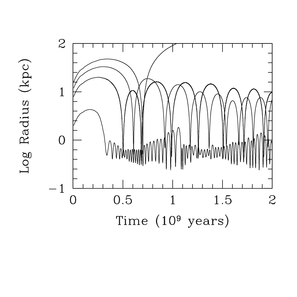
This idealised evolution is illustrated in Fig. 2 for the sphere simulated by 800 spherical shells. This shows the logarithm of the radius of four different shells as a function of time; the largest shell is the outermost shell. It is evident that the shells oscillate with different frequencies and inter-penetrate. Due to the phase mixing, the sphere will eventually come into an equilibrium state. The over-density is calculated by comparing the average density within in the outermost shell to that of the homogeneous Universe at that epoch. This is shown by the dashed curve in Fig. 1 where we see that evolution of follows that of the numerical solution of eq. 3 until and then diverges.
The approach to final equilibrium can be seen by considering the virial ratio () as a function of time. In modified dynamics the gravitational potential is, properly speaking, not defined; an infinite energy is required to move any shell to infinity. None-the-less it is possible to define a virial relation which, in equilibrium, takes the form where is the total kinetic energy as usual and, in spherical symmetry,
(Romatka 1992, Gerhard & Spergel 1994). Here, is the modified gravitational acceleration given by eq. 1. For the system of spherical shells this becomes over all shells. As in Newtonian dynamics the condition corresponds to equilibrium, but, unlike Newtonian dynamics, if the system remains gravitationally bound and will re-collapse.

The virial ratio as a function of time for the sphere is shown in Fig. 3. Initially, there is too much kinetic energy in expansion as would be the case in a low universe; the sphere would never re-collapse in the context of Newtonian dynamics. But with modified dynamics re-collapse and mixing do occur and after roughly three or four dynamical time-scales ( years), the virial ratio approaches one. Fairly significant () oscillations continue for another three to four dynamical timescale– somewhat longer than in Newtonian collapse calculations as found by Ciotti et al. (2007).
The cosmic time and redshift of the initial collapse of objects of different mass is shown in Fig. 4 as a function of mass. The initial conditions and final state of these objects is given in Table 1. The initial collapse is that point where the virial ratio reaches its first maximum corresponding to excessive kinetic energy primarily in tangential motion. We see that initial re-collapse for galaxy mass objects ( ) occurs almost coevally, when the cosmic age is between 50 and 100 million years, or at redshifts between 10 and 20. By redshifts of 8 to 10, these galaxy scale masses would be in place as virialized objects.

For determining the density and velocity distributions the effective number of shells is increased to 8800 by considering the position and velocities of shells at different epochs. The density distribution resembles that of a Jaffe model (Jaffe 1983) having a power law of exponent near 2 in the inner region steepening to more than 3 in the outer regions (we recall that this is also similar to the density distribution in the MOND isothermal sphere: Milgrom 1984, Sanders 2000). The radial velocity dispersion gradually declines as a function of radius, as in the high order polytropic spheres considered by Sanders (2000). This is roughly consistent with decline observed in elliptical galaxies, at least, out to the effective radius.
| Mass ( M⊙) | ( | (kpc) | (km/s) | (km/s) | (kpc) | |
|---|---|---|---|---|---|---|
| (1) | (2) | (3) | (4) | (5) | (6) | (7) |
| 0.05 | 1.66 | 5.6 | 100.2 | 29.1 | 72.1 | 1.75 |
| 0.10 | 1.86 | 7.0 | 135.7 | 20.7 | 95.8 | 3.75 |
| 0.20 | 2.10 | 8.9 | 163.9 | 18.9 | 108.0. | 5.25 |
| 0.40 | 2.37 | 11.2 | 198.0 | 17.0 | 139.4 | 7.0 |
| 0.60 | 2.54 | 12.8 | 221.1 | 16.6 | 155.7 | 8.5 |
| 0.80 | 2.68 | 14.1 | 239.1 | 15.7 | 172.7 | 10.8 |
| 1.0 | 2.78 | 15.2 | 254.0 | 15.0 | 188.3 | 11.5 |
| 2.0 | 3.15 | 19.1 | 306.5 | 13.5 | 231.5 | 16.3 |
| 4.0 | 3.58 | 24.1 | 369.6 | 12.1 | 278.0 | 23.0 |
| 6.0 | 3.86 | 27.5 | 412.3 | 11.4 | 320.7 | 26.8 |
| 8.0 | 4.06 | 30.3 | 445.6 | 10.6 | 346.4 | 30.5 |
| 10.0 | 4.23 | 32.7 | 473.3 | 10.5 | 350.1 | 33.3 |
| 20.0 | 4.82 | 41.2 | 570.4 | 9.2 | 446.3 | 49.5 |
Because of the large collapse factor the final equilibrium form is extremely anisotropic with an effective anisotropy radius of 1 kpc– well within the effective radius. Such objects would probably be highly unstable due to the extreme anisotropy, but this is suppressed here by the imposed spherical symmetry. The non-linear development of this instability would lead to a triaxial figure and a larger anisotropy radius consistent with stability, as is the case in the three-dimensional collapse calculations of Nipoti, Londrillo & Ciotti (2007a). For this reason, the equilibrium objects resulting from these spherically symmetric calculations are not appropriate in detail as models for elliptical galaxies. Nonetheless, it is of interest that the global properties resemble those of the anisotropic polytropes applied previously (Sanders 2000) as models for elliptical galaxies: specifically, a mild deviation from isothermality similar to that of n=12 to n=16 polytropes and a velocity distribution which is increasingly anisotropic in the outer regions.

In Fig. 5 the surface density profiles are shown for the equilibrium figures resulting from four different calculations appropriate to different mass spheres. We see that these profiles are well fit by empirically successful law typically over two orders of magnitude in surface density. The flat central surface density is an artifact of the unrealistically large initial tangential velocity on shells. Significantly, the projected central surface density is constant, and the effective radius grows, roughly, as the square root of the mass. The effective radius is also comparable to the critical radius for modified dynamics (); i.e., galaxy mass objects naturally re-collapse to a radius of about 10 kpc without dissipation.
It is of some interest that spherically symmetric expansion and re-collapse in MOND seems to be capable of producing final virialized objects in which the surface density distribution is a reasonable approximation to a law. With Newtonian dynamics, it is necessary to begin with a highly inhomogeneous, or clumpy, initial density distribution in order to drive the redistribution in phase space sufficient to achieve such a universal surface density distribution; uniform spherical collapse does not work (van Albada 1982). Of course, it is impossible to repeat the calculations described here with Newtonian dynamics because such spheres would be unbound; there would be no re-collapse. But beginning with cold spherically symmetric Newtonian collapse of objects of the same mass and size scale as described here, I find that the final range of phase space covered by the particles is considerably more restricted than for the MOND calculations. The MOND re-collapse produces a number of shells which would be unbound in the context of Newtonian dynamics; this appears to make the critical difference for the final surface density distribution.
Fig. 6 shows the results of the 13 simulations covering a range of masses between and on the log effective radius-log central velocity dispersion plane compared to the observations of Jørgensen et al.[Jørgensen 1999, Jørgensen, Franx & Kærgard 1995a, Jørgensen, Franx & Kærgard 1995b]. In several of these simulations a different value of the initial tangential velocity was assumed ( = 20-40 km/s). Again we see that these global characteristics of objects which condense out of the cosmological expansion via the MOND prescription are generally similar to those of actual elliptical galaxies, although the models are somewhat more inflated than actual elliptical galaxies (larger effective radius for a given velocity dispersion). This suggests that some global dissipation may be necessary to reproduce the observed distribution of real objects on this plane.
Fig. 7 is the mass-velocity dispersion relation for these 13 equilibrium objects; also shown is that of the anisotropic n=12 to n=16 polytropes applied previously (Sanders 2000) as MOND models for elliptical galaxies which reproduce the observed fundamental plane. For the collapse models the velocity dispersion is that along a single line-of-sight toward the centre weighted by density. The observed line-of-sight velocity dispersion within a circular diaphragm, for example of 1.6 kpc diameter [Jørgensen, Franx & Kærgard 1995a], would be about 25% lower.
It is evident that the collapsed spheroids do exhibit a mass-velocity dispersion relation similar to that observed, although they are more homologous than actual ellipticals (less scatter on the Faber-Jackson relation). This is because the spherical collapse model is highly idealised (i.e., no deviation from spherical symmetry or internal structure). These objects would also lie on a fundamental plane similar to that described by the anisotropic polytropes (Sanders 2000, eq. 15) i.e., (the scaling is lower due to the extreme and unrealistic anisotropy). But the important conclusion is that objects resembling the ellipticals do condense out of the Hubble flow within the framework of the MOND scenario for structure formation. Moreover, the final virialized objects attain the mean binding energy of actual galaxies without the necessity of dissipation. These are not deep MOND objects (such as dwarf spheroidals or other low-surface brightness systems) but are more similar to average massive ellipticals which are Newtonian within an effective radius. (Deep MOND isothermal spheres with large constant density cores are possible configurations, but not by this formation scenario; Milgrom 1984, and private communication.)
In summary, objects formed from MOND dissipationless collapse exhibit well-defined radius-velocity dispersion and mass-velocity dispersions relationships. These are of the form
and
where (shown by the solid lines in Figs. 6 and 7. These objects differ from pure isotropic, isothermal spheres where and (Milgrom 1984, Sanders 2000). Significantly, this means that such objects also have a characteristic density which is also related only to the velocity dispersion:


4 The MOND condition for fragmentation
These dissipationless calculations still do not address the question of why galaxies of stars seem to be restricted to mass of less than . For this we have to consider cooling and fragmentation processes which lead to star formation.
In the traditional picture, this process is considered in terms of two competing timescales– the dynamical time vs. the cooling time. Presumably, the elements of the collapsing cloud collide, heat up, and attain a temperature appropriate to the virial velocity dispersion. The radiative cooling timescale of this hot plasma is
where is the temperature, is the mean molecular weight, the mass of the proton, the density, and is the cooling rate per hydrogen nucleus in a plasma having specified, presumably primordial, abundances. With Newtonian dynamics, the dynamical, or collapse, timescale is
where is the density.
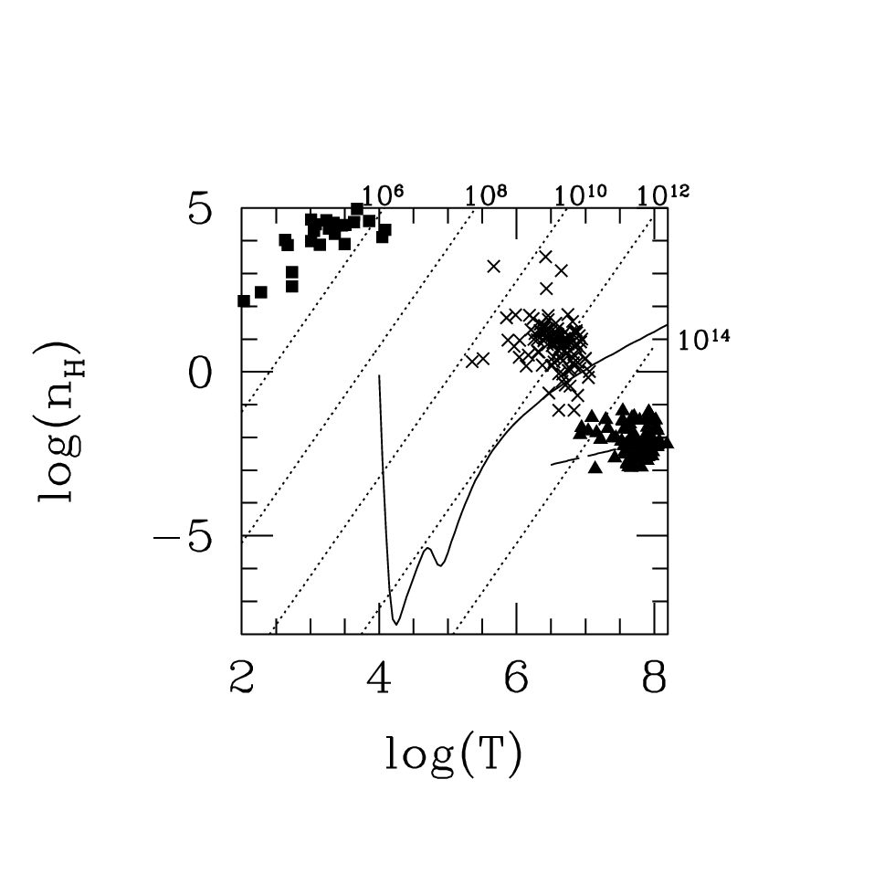
Fig. 8 is a density-temperature plane for a hypothetical gas cloud and the solid curve shows the locus where . Above the solid curve, one would expect cooling, fragmentation and star formation to play an important role. The points on the curve show three classes of pressure supported systems: globular clusters (Pryor & Meylen 1993, Trager et al. 1993), elliptical galaxies [Jørgensen 1999, Jørgensen, Franx & Kærgard 1995a, Jørgensen, Franx & Kærgard 1995b] and X-ray emitting clusters of galaxies (White, Jones & Forman 1997). The point made by numerous authors (e.g., Silk 1977) is clear: Those objects consisting primarily of stars, ellipticals, are above the curve; whereas clusters of galaxies, consisting primarily of hot gas, are below.
If we consider gas clouds uniformly mixed with a dark matter halo in virial equilibrium we can also define a relation between the mean density and the temperature for a given dark matter mass:
where is a number depending upon the density distribution in the cloud and () is the baryon to dark matter density ratio,. This density-temperature relation is also shown in Fig. 8 for objects of the indicated total dark mass. The point is that for objects with the virialized cloud will lie primarily in the region where cooling is slow compared to the collapse timescale. In this region we would expect that the fragmentation to the level of individual stars does not occur before subsequent dynamical evolution of the object.
With MOND we have seen that dissipationless objects which condense out of the Hubble flow exhibit a well defined radius-velocity dispersion, mass-velocity dispersion relations (eqs. 10 and 11) which imply a density-velocity relation (eq. 12). However, the initial re-collapsing object, at maximum expansion, is certainly a gas cloud; as the cloud collapses subcomponents will collide and, most likely, generate a temperature with thermal velocity comparable to the random velocity of components. Therefore, a critical assumption here, as in the standard model, is that the gas virial temperature generated during re-collapse, fragmentation, and star formation is essentially given by the random velocity of the virialized object. For our hypothetical gas cloud, therefore, the radius-temperature and mass-temperature relations corresponding to eqs. 10 and 11 are (for )
where I have taken the mean atomic weight of 0.62 for an ionised gas with primordial abundances. The dynamical timescale for the cloud would therefore be or
Expressing the characteristic density of a collapsed object (eq. 12) in terms of the hydrogen density for a fully ionised plasma with primordial abundances:

The condition where now is defined by eq. 18 is shown by the solid curve in Fig. 9. The three classes of self-gravitating objects are are indicated here as is Fig. 8. The temperature of the gas clouds with indicated masses, as given by eq. 17, is now shown by the vertical dotted lines (there is no dependence on scale, and hence density, in the MOND virial relation). And finally, the characteristic MOND density (eq. 19) for a near-isothermal cloud in equilibrium is shown by the dashed line.
We see that the solid curve again separates those objects built primarily from stars (elliptical galaxies) from objects consisting primarily of gas (clusters). We also see that the MOND density-temperature relation intersects this curve for an object with a mass of about . This means that objects which are more massive will have a density and temperature such that cooling and fragmentation occurs on a timescale longer than subsequent evolution of the system as a whole; this provides a natural upper limit for objects built of stars. It is also evident that actual virialized systems do cluster about the line of the characteristic MOND density. This has been pointed out previously in other contexts (Sanders & McGaugh 2002).
If cosmological neutrinos have a mass of 2 eV they will comprise the dark component of clusters required even in the context of MOND (Sanders 2003). In this case the neutrino fluid will become a dominant component of clusters at temperatures higher than about K, and the curve of would steepen at higher temperatures (Sanders 2007). This does not affect the argument on fragmentation. If the dark component of clusters is baryonic (Milgrom 2007), then the form of the curve remains the same.
At high temperature, the solid curve in Fig. 9 () appears to approach a constant value of the density. This is because the cooling timescale for a high temperature plasma is set by free-free emission and is given by
where is a numerical constant, is the mass of the electron, is the Thompson radius () and is the fine structure constant (). That is to say, the cooling timescale is proportional to , as is the dynamical timescale (eq. 18). Therefore, the temperature drops out of the condition in this high temperature regime; there is a characteristic density where this condition is met of cm-3. Equating this to the MOND density for a virialized system (eq. 19) then defines a characteristic temperature or (from eq. 17) a mass. This mass would be the upper limit to an object where fragmentation to stars has proceeded– the characteristic galaxy mass. This turns out to be
where is the gravitational coupling constant. Therefore, with MOND, as in the standard paradigm, the galaxy mass is defined in terms of fundamental constants although, in our case, enters into the expression. Given that, coincidentally, , eq. 15 becomes
which is similar (but not identical) to the expression derived by Silk (1977).
5 Conclusions
It has been appreciated for many years (e.g. Binney 1977) that, by the mechanism of gravitational instability in an expanding Universe, it is impossible to form the luminous parts of galaxies without dissipation. This remains true in the context of the current cosmological paradigm, CDM. Given the amplitude of fluctuations on galaxy scale at decoupling, bound objects of would form at a redshift of about 5 with a characteristic scale of to 20 to 50 kpc (defined as the radius at which the power law density distribution breaks from -1 to -3) and a density between and gcm-3– independently of whether or not they form hierarchically or by monolithic collapse. (Navarro, Frenk & White 1997). But this would be the presumed characteristic density of dark matter. If the baryonic matter were distributed in the same way (no dissipation) then its density would be 10 times lower. The baryonic matter must dissipate, radiate its kinetic energy and collapse by a further factor of 10 to produce the observed baryonic density in the inner luminous regions of galaxies. Moreover, this dissipation must be global; fragmentation to the level of stars before collapse would not produce galaxies of the observed surface brightness.
With MOND, given the simple ansatz that the modified gravity only applies to fluctuations, this is not true. Then, in a pure baryonic Universe, galaxy scale fluctuations separate out of the Hubble flow early () and re-collapse and virialize by a redshift of 10. The mean surface density and binding energy of these collapsed objects is comparable to that of observed galaxies. The standard surface brightness distribution for ellipticals, the law, is reproduced as well as the Faber-Jackson and Fundamental Plane correlations. This is all accomplished without dissipation. Of course, galaxies are self-gravitating ensembles of stars. So, to form galaxies in this dissipationless limit, cooling and fragmentation to the level of stellar mass objects must occur on a timescale short compared to the collapse time. Therefore, as in the standard picture, radiative cooling must set the mass scale of galaxies.
The more robust result here, independent of the ansatz on structure formation, concerns the properties of protogalactic clouds. With MOND, unlike the Newtonian case, an acceleration scale enters the structure equation. This means that a near isothermal object with a given velocity dispersion, or temperature, will have definite mass: if that velocity dispersion is 100-200 km/s the mass will be on the order of Moreover, there also is a definite size scale associated with an isothermal object of a given mass– and that is the radius of the transition from Newtonian dynamics to modified dynamics. The isothermal object will inflate to this radius and thereafter truncate. This implies the existence of a characteristic density which can be identified with a particular mass; for example, a mass of will have a density of about one particle per cubic centimetre. For lower masses, or temperatures below K, the virialized MOND clouds lie in the domain where cooling is more rapid than collapse; here we expect the cloud to fragment and form a galaxy of stars essentially by dissipationless collapse. For higher temperatures this is no longer the case. The cloud may well maintain its identity as a gaseous object until merging with a similar cloud as part of a larger collapsing structure. It is of interest that observed pressure supported, near isothermal objects do, at present, lie near the characteristic MOND density-temperature relation.
In summary, with MOND galaxy scale masses are likely to re-collapse and virialize early (). Spherically symmetric N-body calculations indicate that the objects which condense out of the Hubble flow, resemble actual elliptical galaxies. This suggests that elliptical galaxies may form by monolithic collapse without global dissipation. The condition that cooling takes place rapidly compared to collapse, as in the standard scenario, places an upper limit of about on those bound objects which can consists primarily of stars.
I am grateful to Françoise Combes, Stacy McGaugh, and Moti Milgrom for very helpful comments on this paper. I also thank the referee, Pasquale Londrillo, for a number of very usful comments and criticisms which greatly improved the content and presentation of this paper.
References
- [Bekenstein 2004] Bekenstein J.D. 2004 Phys.Rev.D, 70, 083509
- [Bekenstein & Milgrom 1984] Bekenstein, J.D. & Milgrom, M. 1984, ApJ, 286, 7
- [Binney 1977] Binney J. 1977, ApJ, 215, 483
- [Binney & Tremaine 1987] Binney, J. & Tremaine, S. 1987, Galactic Dynamics, Princeton Univ. Press (Princeton).
- [Blumenthal et al. 1984] Blumenthal G.R., Faber S.M., Primack J.R., Rees M.J. 1984, Nature, 311, 517
- [Ciotti, Nipoti & Londrillo 2007] Ciotti L., Nipoti C., Londrillo P., preprint, astro-ph/0701826
- [de Vaucouleurs 1948] de Vaucouleurs G. 1948, Ann.Astrophys., 11, 247
- [Faber & Jackson 1976] Faber, S.M., & Jackson, R.E. 1976, ApJ, 204, 668
- [Felton 1984] Felten, J.E. 1984, ApJ, 286, 3
- [Gerhard & Spergel 1992] Gerhard, O.E. & Spergel, D.N. 1992, ApJ, 397, 38
- [Hénon 1964] Hénon, M. 1964, Ann.d’Astroph., 27, 83
- [Hoyle 1953] Hoyle F. 1953, ApJ, 118, 513
- [Jaffe 1983] Jaffe, W. 1983, MNRAS, 202, 995
- [Jørgensen 1999] Jørgensen, I. MNRAS, 306, 607
- [Jørgensen, Franx & Kærgard 1995a] Jørgensen, I., Franx, M. & Kærgard, P. 1995a, MNRAS, 273, 1097
- [Jørgensen, Franx & Kærgard 1995b] Jørgensen, I., Franx, M. & Kærgard, P. 1995b, MNRAS, 276, 1341
- [Milgrom 1983a] Milgrom, M. 1983, ApJ, 270, 365
- [Milgrom 1984] Milgrom, M. 1984, ApJ, 287, 571
- [Milgrom 2007] Milgrom, M. 2007, preprint, arXiv:0712.4203
- [Navarro, Frenk & White 1007] Navarro J.F., Frenk C.S., White S.D.M. 1997, ApJ, 490, 493
- [Nipoti, Londrillo & Ciotti 2007a] Nipoti C., Londrillo P., Ciotti L. 2007a, ApJ, 660, 256
- [Nipoti, Londrillo & Ciotti 2007b] Nipoti C., Londrillo P., Ciotti L. 2007b, MNRAS, 381, L104
- [Nusser 2002] Nusser A. 2002, MNRAS, 331, 909
- [Pryor & Meylan 1993] Pryor, C. & Meylan, G. 1993, in Structure and Dynamics of Globular Clusters, APS Series V. 50, p. 357
- [Rees & Ostriker 1977] Rees M.J., Ostriker J.P. 1977, MNRAS, 179, 451
- [Romatka 1992] Romatka, R. 1992, PhD. thesis, Max Plank Inst. Phys.
- [Sanders 1996] Sanders R.H. 1996, ApJ, 473, 117
- [Sanders 1998] Sanders R.H. 1998, MNRAS, 296, 1009
- [Sanders 2000] Sanders R.H. 2000, MNRAS, 313, 767
- [Sanders 2003] Sanders R.H. 2003, MNRAS, 342, 901
- [Sanders 2005] Sanders R.H. 2005, MNRAS, 363, 459
- [Sanders 2007] Sanders R.H. 2007, MNRAS, 380, 331
- [Sanders & McGaugh 2002] Sanders R.H., McGaugh S.S. 2002, ARA&A, 40, 263
- [Silk 1977] Silk J. 1977, ApJ, 211, 638
- [Stachniewicz & Kutshera 2005] Stachniewicz S., Kutshera M., 2005, MNRAS, 362, 89
- [Trager et al. 1993] Trager, S.C., Djorgovski, S. & King, I.R. 1993 in Structure and Dynamics of Globular Clusters, APS Series V. 50, p. 347
- [van Albada 1982] van Albada, T.S. 1982, MNRAS, 201, 939
- [White & Rees 1977] White S.D.M., Rees, M. 1978, MNRAS, 183, 341
- [White, Jones & Forman 1997] White D.A., Jones C., Forman W. 1997, MNRAS, 292, 419
- [Zhao & Famaey 2006] Zhao H.S., Famaey B., 2006, ApJ, 638, L9
- [Zlosnik, Ferreira & Starkman 2006] Zlosnik T.G., Ferreira P.G., Starkman G.D. 2006, Phys.Rev.D 74, 044037