On Contamination and Completeness in Lyman Break Galaxy SurveysOn Contamination and Completeness in Lyman Break Galaxy Surveys–References
Abstract
A large population of Lyman break galaxies has been identified in recent years. However, the high redshift galaxies selected by different surveys are subject to a variety of selection effects - some overt, others more subtle. We present an analysis of sample completeness and contamination issues in high redshift surveys, focusing on surveys at and using a spectroscopically-confirmed low redshift sample from the DEEP2 survey in order to characterise contaminant galaxies. We find that most surveys underestimate their contamination from highly clustered galaxies at and stars. We consider the consequences of this for both the rest-frame ultraviolet luminosity function and the clustering signal from galaxies. We also find that sources with moderate strength Lyman- emission lines can be omitted from dropout surveys due to their blue colours, again effecting the derived luminosity functions. We discuss the points of comparison between different samples, and the applicability of survey-specific results to the population at in general.
Keywords:
galaxies: high-redshift, evolution, luminosity function; techniques: photometric1 Introduction
The study of galaxies has become a well-developed field in recent years. The Lyman Break (or ‘dropout’) technique - which identifies starbursting sources by the dramatic spectral break around the rest-frame Lyman-alpha feature and was first applied at (Steidel et al. 1999) - is now widely applied on large multicolour datasets. As a result, large samples of photometrically-selected high-redshift candidates can be constructed with a comparatively small investment of telescope time. Such photometric samples have been widely used to derive statistical properties for galaxies as a whole, including luminosity functions and clustering parameters. (Ouchi et al. 2004b; Iwata et al. 2007; Lee et al. 2006)
However, the high redshift galaxies selected by different surveys are subject to a variety of selection effects - some overt, others more subtle. While samples of Lyman- emitting galaxies (selected over a narrow redshift range, and relatively easy to confirm spectroscopically due to the presence of strong emission lines) have comparatively simple selection windows (see Hayes & Östlin 2006, for discussion), the variety in width and shape of broadband filters leads to a wide range of redshifts (and hence intrinsic luminosity limits) falling into the selection window, while the presence or absence of emission lines can alter the effectiveness of a colour selection. Such effects are highly sensitive to filter profile, selection criteria and survey depth. Although attempts to interpret the results of photometric surveys have generally considered each such survey comparable, these sample-specific issues relating to completeness and contamination can alter the resulting physical interpretations. The situation is complicated by the fact that the dominant contaminant populations have not hitherto been carefully and systematically characterised.
While most surveys take into account a subset of these effects, the description of published data is in many cases inadequate to allow comparison between results. In this paper, we present an analysis of significant sample completeness and contamination issues in high redshift surveys based on the Lyman break technique, focusing on the galaxy population at to illustrate the complexity of the situation. We discuss the points of comparison between different samples, and the applicability of survey-specific results to the population at in general, pulling together the modelling and observational results to construct a coherent picture of the high redshift population under examination. An understanding of these issues is essential to allow fair comparison between different datasets, between data and theory and when planning future surveys.
In section 2 we consider the selection effects that can influence a high redshift survey and in section 3 we describe the contaminant populations that also show dropout colours. In section 4 we discuss the consequences of these effects on the interpretation of published results from high redshift surveys, and the implications for the design of future surveys.
Throughout the paper, we consider filter sets and selection functions that have been applied to existing Lyman break galaxy surveys. The instruments and filter sets considered, together with examples of relevant surveys are shown in table 1 and illustrated in figures 1 (filter profiles) and 2 (colour selections). While these selection functions do not form constitute an exhaustive list, they are indicative of the variation from survey to survey11 1 Note, we don’t discuss the UKIDSS selection of McLure et al. 2006 in detail since the colour cut excludes galaxies and renders this more properly an -drop selection. Hence the UKIDSS survey expects sources at much lower surface densities making it not comparable to other surveys.. Where appropriate, we adopt the following cosmology: a flat Universe with , and . All magnitudes (optical and infrared) are quoted in the AB system (Oke & Gunn 1983).
| Facility | Filters Used | Selection Criteria | Examples |
|---|---|---|---|
| HST/ACS | F435W(), F606W(), F775W(), F850LP() | Bremer et al. 2004; Verma et al. 2007 | |
| VLT/FORS2 | (ESO 74), (ESO 76), (ESO 77), (ESO 78) | Douglas et al (in prep), Lehnert & Bremer 2003 | |
| Subaru/Suprime-Cam | , , , , |
, &
|
‘Viz’: Ouchi et al. 2004a, Yoshida et al. 2006 |
|
, &
|
‘Riz’: Ouchi et al. 2004a, Yoshida et al. 2006 | ||
| CFHT/Megacam | , , , | None as yet |


2 Completeness Issues in Dropout Samples
2.1 Redshift Completeness and Number Counts
The majority of surveys published in the literature fall into two categories. Sources are selected either for the presence of a strong emission line, detected as excess emission in narrowband imaging(Hayes & Östlin 2006, not discussed further here, see), or by the break in their continuum emission. In the latter case, the selection is based on an extreme colour in a single pair of filters, often refined by constraints in one or more additional bands. In the case of galaxies at , the selection criteria applied in most surveys is either based on colour or on , depending on available imaging, with a constraint on often applied a posteriori in order to reduce sample contamination (see section 3).
The requirement for an extreme colour sets a firm lower limit to the redshift of a survey, while the width of the selection filters defines the redshift range. In theory, the simplicity of this approach should allow samples selected using the same colour cuts on different instruments to be compared directly.
However such comparisons overlook one significant factor: not all filter sets are equivalent. There has been a proliferation of filter sets in the optical, each designed to optimise source signal to noise, but approaching the problem in different ways. Such filters are assigned common names of , , and (or variants on these) on the basis of their effective wavelength, but often differ significantly in terms of width, filter response22 2 combining filter transmission profile with available information on CCD and instrumental response. and overlap with neighbouring filters. This has little effect on the measured magnitudes in each band of sources with smooth profiles, but can significantly impact the measured colours of spectra dominated by sharp features such as continuum breaks.
As figure 3 illustrates, a single high redshift galaxy (Madau 1995, in this case modelled as a source flat in , appropriate for young starbursts, and modulated by the intergalactic hydrogen opacity as a function of redshift given by), can have dramatically different colours in different filter sets. A single colour cut simply cannot be applied uniformly to different filter sets since the resulting redshift ranges can differ by , particularly if -drops are compared with sources selected as -drops.
This simple fact is widely understood in the observational community and most surveys account for this effect by varying their selection criteria accordingly as shown in table 1 to tune the minimum redshift satisfying the colour selection. Nonetheless, the redshift range probed still varies from sample to sample due to the width of, and overlap between, the filters available to them.
The most dramatic effect of this redshift variation from survey to survey arises not from the redshift evolution of the population itself, but rather from the simple change in luminosity distance over the redshift range in question. For a magnitude-limited sample, a progressively brighter limiting luminosity is reached in each successive redshift slice. Given the relatively steep faint-end luminosity function observed for Lyman break galaxies at , a small reduction in survey depth at any given redshift can have dramatic effects on the number of galaxies predicted in that bin.
The combination of these effects - filter response, subsequent redshift selections and the luminosity bias towards low redshifts - and their effect on predicted number counts is illustrated in figure 4. For a constant luminosity function (i.e. a non-evolving population from ) the number of galaxies predicted as a function of redshift is shown for each of the selection criteria in table 1.
While the two -drop samples considered here (the selection functions generally applied to Subaru and HST/ACS data) overlap significantly in redshift with the -drop samples, allowing both groups to be called ‘ Lyman Break galaxy populations’, the surface density of sources observed by such samples is some two times higher. Similarly, there are clear variations within the -drop samples. The ‘Riz’ selection utilised by the Subaru Deep Field (SDF) for example, will identify sources at lower redshifts than that applied by the ERGS survey at the VLT, but will miss 40% of Lyman break galaxies with the same continuum magnitude at .
Also notable is the role played by photometric error in the redshift distribution. As figure 3 illustrated, it is possible for the dropout colour to remain static with redshift in some filter sets (due either to filter overlaps or to significant offsets between the and filters). If the selection criteria is set close to such a plateau, then Gaussian scatter in both the intrinsic colour of the sources and the photometry will promote a fraction of the more abundant population from lower redshifts into the sample, while simultaneously scattering a fraction of higher redshift sources blueward of the limiting colour. The result is a redshift distribution that bulges below the nominal selection cutoff, as seen in figure 4 for both the VLT/FORS2 and CFHT/MegaCam selection criteria. It is interesting to note that this effect will be present for any selection criteria based largely on a single colour, affecting Lyman-break galaxies across a range of redshifts, as well as the Distant Red Galaxy population (Franx et al. 2003, DRGs, )
Figure 4 is plotted for the luminosity function determined by Steidel et al. 1999 for Lyman break galaxies at . This luminosity function is known to overpredict the number of sources of bright magnitudes (Lehnert & Bremer 2003), and hence the predicted number counts in figure 4 should be considered indicative rather than precise. However, while the normalisation of figure 4 may change, the basic differences in the redshift distributions of sources will remain unless the shapes of those distributions also change.
Altering the luminosity function parameters has no effect on the colours of a high redshift source (which are fixed by rest-frame UV slope and Lyman- forest transmission), but does effect the number of sources in a given volume which will satisfy this criterion. Decreasing the typical luminosity L* to half its value at reduces the peak number density of sources by a factor of six, but affects the shape less severely, broadening the redshift distribution at FWHM by approximately 10%. Similarly, increasing the faint end slope from -1.5 to -1.9 has the effect of decreasing the peak number density by 15% while leaving the shape and FWHM of the distribution unchanged.
Hence the primary effect is on the normalisation rather than the shape of the redshift distribution and the filter-to-filter comparison discussed here are largely independent of luminosity function.
The effect of changing the limiting luminosity of a survey is rather more pronounced. Such a change does not alter the minimum redshift identified by the survey but does increase the depth relative to L* in each successive redshift bin. Since the luminosity function is steep at the faint end, this has the effect of broadening the redshift distribution in a given filter set and extending the tail of the function to higher redshifts.


2.2 Effect of Line Emission
Lyman break galaxy surveys focus on the analysis of galaxies detected through their rest-frame ultraviolet continua. However, it is known from Lyman- emitter surveys (Ajiki et al. 2006; Hu et al. 2004; Malhotra & Rhoads 2004, e.g.) that there exists a significant population of sources with powerful emission lines at Å, a fraction of which overlaps with the Lyman break galaxy population. At , a quarter of all spectroscopically confirmed Lyman break galaxies show Lyman- emission with a rest-frame equivalent width of Å, while a second quartile has Å (Shapley et al. 2003).
Figure 5 illustrates the effect of moderate line emission on the colours of a flat-spectrum continuum-source, for one example filter set - in this case, the VLT/FORS2 filters. As in most surveys, a flat-spectrum galaxy will satisfy the VLT/FORS2 selection criterion at redshifts where the Lyman- feature is in the -band. While this remains true, increasing line strength has the effect of reducing the galaxy colour and dropping it out of the sample at the low redshift end of the selection function. At higher redshift, the presence of a line-emitting population has the effect of scattering galaxies over a much broader region than the simple galaxy locus, potentially reducing the ability of a survey to reliably separate galaxy loci from contaminants (see section 3).
A second effect of line emission is to increase the observed magnitude of a galaxy when compared to an equivalent continuum source without line flux. At faint magnitudes, a moderate strength emission line can contribute a large fraction of the observed broadband flux, particularly at high redshifts (since only a small fraction of the filter is free of Lyman- forest line dampening). Given the steep faint-end slope expected for any reasonable luminosity function, the population of galaxies just beyond the (continuum) magnitude limit of a survey is larger than the faintest population above the limit. Hence a small fraction of those galaxies, entering the sample due to the presence of strong emission lines, can skew both redshift and equivalent width distributions.
Stanway et al. 2007 recently found evidence for a tail of high equivalent width sources in a faint Lyman break galaxy sample at from the Hubble Ultra Deep Field (Beckwith et al. 2006), suggesting that the effect of strong line emission on the tail of the galaxy distribution could be measurable in a larger sample at equivalent faint limits.
Each of these effects will be dependent on the position of Lyman- emission relative to the filter edges, and also on the detailed profile of those filters. A filter with a square-edged transmission profile will have clear advantages in terms of reducing the tail of galaxies that are detected in spectral regions with very little filter throughput. However the decline in throughput of optical CCDs through the -band leads to an inevitable blurring of the edges, and square-transmission filters will not prevent effects arising from incomplete blanketing of one or more bands by Lyman- forest absorption.

2.3 Effect of Spectral Slope and Burst Age
By contrast, intrinsic spectral slope has a relatively small effect on the colours of high redshift galaxies, which are dominated instead by the effects of interstellar absorption. Nonetheless, a blue rest-frame ultraviolet spectral slope (appropriate for young sources) might reasonably be associated with strong line emission, and so will strengthen the effect seen above. The effect of varying the ultraviolet spectral slope (in the absence of line emission) is shown in figure 6. The effects of a bluer average ultraviolet continuum at (Stanway, McMahon, & Bunker 2005, possibly steeper than , see) compared with the lower redshift population (Steidel et al. 1999, typically ,) are unlikely to have a big impact on the selection since they are of the same order as photometric errors at these faint magnitudes, but could produce a measurable effect for sources close to the selection limits.

The most significant factor driving the rest-UV spectral slope is the age of the current starburst in a galaxy. The hottest, most-massive stars provide the largest contribution to the rest-frame ultraviolet, and these stars also have the shortest lifetimes. As a result, the optical colours of galaxies at evolve with the age of the galaxies in question.
In figure 7 we explore the effect of changing the template SED on the selectability of high redshift galaxies, with particular reference to the Subaru -band colour selection in table 1. The colours of a spectrum flat in is compared with those predicted by stellar population synthesis models for galaxies constant star formation over the preceding 10 Myr and 100 Myr (assuming solar metallicity and a Salpeter IMF). We consider the results of two different stellar synthesis codes for identical output parameters. The Bruzual & Charlot 2003 codes have been the most widely used synthesis models in recent years and were utilised by Ouchi et al. 2004a to estimate the photometric selection criteria for high redshift galaxies. They produce redder model colours at a given redshift than the newer stellar synthesis models of Maraston 2005, which incorporate improved treatment of the thermally-pulsating asymptotic giant branch phase (Bruzual 2007, see).
Evidence from SED fitting to the stellar populations in galaxies (Verma et al. 2007; Stark et al. 2007; Eyles et al. 2005) has determined that the majority of this population comprise either young starbursts (50 Myr) or young starbursts with an underlying older ( 200Myr) population that no longer contributes significantly to the rest-UV. In either case, no compelling evidence has been found for continuous star formation over timescales of 100 Myr. This youth of stellar populations at high redshift is supported by other work (Lehnert & Bremer 2003; Stanway, McMahon, & Bunker 2005; Pentericci et al. 2007, see), which finds colours consistent with a flat spectrum in bands uncontaminated by the break in samples.
For the purposes of this paper we adopt a spectrum flat in (i.e. ) as being a simple template galaxy. As figure 7 illustrates, this is appropriate for young starburst populations (in the Maraston 2005, models), although we note that uncertainties in the star formation history can lead to variation in colour by approximately 0.1 mag (or less than the photometric scatter in a typical survey of faint dropouts).

2.4 UV-faint Galaxies
The dropout selection technique, by its very nature, identifies sources with a bright rest-frame ultraviolet continuum. Ultraviolet flux is contributed primarily by young, short lived stars - hence the use of Lyman break selected samples to gauge the star formation history of the universe (Madau et al. 1996; Steidel et al. 1999; Bouwens, Broadhurst, & Illingworth 2003; Stanway, Bunker, & McMahon 2003).
However, the ultraviolet continuum flux declines sharply with increasing time after an instantaneous starburst (Leitherer et al. 1999), varying by three orders of magnitude in the first 100 Myr. Hence the Lyman break technique cannot identify galaxies at high redshift that have passed through a starburst and are now passively evolving since such sources will no longer have a strong ultraviolet continuum. At a 100 Myr-old starburst would have peaked at only and yet may be undetectable by dropout selection (unless star formation continues throughout this time).
Similarly, it takes a finite time after a starburst for an ultraviolet continuum flux generating population to become established, causing very young starbursts (5 Myr) to be detectable primarily in emission from the Lyman- emission line. Hence both very young and very old starbursts may be omitted from a dropout survey, while galaxies of Myrs in age may be preferentially selected based on ultraviolet flux.
Whenever only isolated subsets of the total galaxy population is observed, it is possible to miss aspects of the bigger picture. Populations that are small in number - such as the DRG galaxies (a combination of old and dusty galaxies) at - can make non-negligible contributions to important cosmological parameters such as the galaxy metal budget (Bouché, Lehnert, & Péroux 2006) and stellar mass density (Marchesini et al. 2007). Hence it is important to consider constraints on galaxies not selected by high redshift dropout samples.
An analogue to the passively evolving subset of DRGs at would be old sources without significant ongoing star formation. In these old galaxies, the most easily detected spectral feature would be the rest-frame 4000Å break. Mobasher et al. 2005 have proposed that infrared data can be used to detect the Balmer break in galaxies. Although their initial candidate may well lie at lower redshifts, the technique has now identified a small number of candidate galaxies at comparatively bright magnitudes (Chary et al. 2007; Rodighiero et al. 2007; Dunlop, Cirasuolo, & McLure 2007). Unfortunately a degeneracy in observed optical-infrared colour between dusty galaxies and non-starforming galaxies renders the analysis of such a population based on photometric redshifts alone difficult. Photometric redshifts in the available broad wavebands can favour one solution, but not to the exclusion of the other, and quantitative results cannot be drawn without appropriate caveats and speculative corrections. Detailed investigation of high redshift galaxies without significant rest-UV flux will most likely require a future generation of telescopes and instruments capable of performing rest-frame optical spectroscopy on extremely faint sources.
The importance of this population is difficult to quantify. If the most massive sources collapsed earliest then old galaxies could conceivably be amongst the brightest high redshift sources and hence retain a measurable ultraviolet flux to any given magnitude limit despite the rapid decline of ultraviolet emission after its initial peak. Many old galaxies at may also have ongoing star formation and so examples have been identified as high redshift sources on the basis of recent starburst activities rather than through their evolved populations (Eyles et al. 2005, e.g.). The population of old galaxies not-selectable as - or -drops may be constrained through measurements of star formation at , but before that is necessarily a matter of speculation.
In addition to incompleteness in terms of old, massive galaxies, Lyman-break samples may also be incomplete for young galaxies of similar mass to those observed. Verma et al. 2007 fitted the optical and ultraviolet spectral energy distributions of -band dropouts, and determined that the typical age of such galaxies is Myr, with approximately one third of the sample showing evidence for underlying older ( Myr) starbursts. While there is clearly a bias against old galaxies when selecting on unobscured ultraviolet luminosity, an intermediate age population of Myr starbursts should have been easily detected. As Verma et al. 2007 discuss the presence of such a large population of short-lived sources distributed throughout the comparatively long (325 Myr) time span probed by the sample suggests that the detected galaxies represent a more passive population an order of magnitude more numerous that shows stochastic bursts of star formation.
Neither of the above selection effects accounts for the additional effect of dust extinction, which can suppress the rest-frame ultraviolet flux. At lower redshifts () several species of dust-obscured galaxies are known including sub-millimetre galaxies and ultra-luminous infrared galaxies (ULIRGS). The generally blue rest-frame UV slope at (Stanway, McMahon, & Bunker 2005; Bouwens et al. 2006, e.g.) suggests that dust extinction at high redshifts may be lower than those observed at . A dust extinction curve derived from observations of quasars (Maiolino et al. 2004) suggests that high-redshift dust is generated primarily in supernovae and produces up to a magnitude less extinction in the ultraviolet than the more-processed dust seen at lower redshift. The same extinction curve provides a good fit to the spectrum of a gamma ray burst that also lies at (Stratta et al. 2007). If these results are typical of galaxies at high redshifts, then the population lost to dust extinction down to any given magnitude is likely to be smaller than that at lower redshifts, although the presence of sub-millimetre galaxy analogues cannot be ruled out, and mildly dust-obscured dropouts could be a significant cause of incompleteness at the faint end of any survey.
Sample incompleteness over the sensitive redshift range of Lyman-break samples is dominated by the unobscured rest-frame ultraviolet flux and the strength of spectral breaks, and hence are less filter-dependent than those discussed above. These effects are, however, significantly harder to quantify since they rely on the existence of a population that has never actually been observed.
3 Contamination Issues in Dropout Samples
Two distinct populations of astronomical objects - intermediate redshift elliptical galaxies and cool Galactic stars - are degenerate in colour with high redshift galaxies.
While many such contaminants can be distinguished through the use of data in the Spitzer/IRAC bands longwards of 3 m, such imaging is not always available, and in many cases is impossible to obtain because of source confusion at long wavelengths. Similarly, a spectroscopically complete Lyman-break survey can accurately correct for contamination effects, but this realistically limits such a survey to limits of or brighter on an 8m telescope.
Hence understanding and correcting for these contaminant populations is vital when interpreting a photometrically selected sample, particularly at faint magnitudes.
3.1 Cool Galactic Stars
Cool galactic stars of classes M4 and later are routinely selected in dropout selections. M class stars satisfy or -drop colours, while L and T stars have -drop colours (figure 8).
In fields with HST/ACS imaging, stars are routinely excluded on the basis of their unresolved full-width half-maxima33 3 While this risks omitting compact galaxies, all confirmed galaxies thus far observed from space are resolved.. However this approach cannot be used in wide-field imaging, since all known (unlensed) galaxies are unresolved from the ground. Instead the usual approach adopted (Ouchi et al. 2004a, e.g. the Subaru Deep Field studies, ) attempts to exclude stars on the basis of detected flux shortwards of the nominal Lyman- break or through placing constraints on a second colour such as .
As figures 8 and 9 illustrate, the reliability of such a technique depends both on the depth of the imaging available and the metallicity of the stellar population.
In figure 8 the spectra of M and L class stars (Hawley et al. 2002, constructed from a relatively bright sample in the Sloan Digital Sky Survey or SDSS, ) are convolved with the filter profiles of HST/ACS and those used by VLT and Subaru surveys. While the colours of cool galactic stars are less extreme than the technically infinite colour of high redshift galaxies in these bands, they can nonetheless reach very large colour decrements. To reliably exclude faint stars from a survey reaching would require -band imaging some five magnitudes deeper than the survey -band limit. For example, given the limit of the Subaru Deep Field selection of Ouchi et al. 2004a, band imaging to would be required to reliably eliminate the majority of late M and early L class stars from the selection. The actual limiting depth of the Subaru Deep Field is insufficient to reliably exclude stars with -drop colours. However, there is a small redshift region around in most filter sets which should be clear of stellar contamination if the SDSS stellar templates are representative of stars at fainter magnitudes.
Stanway et al. 2007b discuss the properties of a sample of M-stars selected as unresolved -band dropouts () using deep HST/ACS imaging of the Great Observatories Origins Deep Survey (Giavalisco et al. 2004, GOODS, ) reaching a limit of . The optical and infrared (and, for a subsample, spectroscopic) properties of these unresolved sources were studied and found to be consistent with those of stars and inconsistent with those of high redshift galaxies. Stars at the faint magnitudes probed by high redshift surveys are likely to lie at large heliocentric distances and well out of the plane of the galactic disk. Thus a halo origin and sub-solar metallicities is likely to be a reasonable model for such stars. Spectroscopic results for faint -stars are consisted with slightly sub-solar metallicities, and a metallicity spread between solar and a tenth solar (Stanway et al. 2007b, both photometrically and spectroscopically,), a range which can change the colours of late M stars by 0.4 magnitudes in both and (figure 9). Importantly, at early M subtypes, the effect of sub-solar metallicity is to produce bluer colours, and a unresolved sources in the GOODS fields were found to lie 0.1 magnitudes bluewards of the stellar locus expected for SDSS stars with similar colours. Hence even a cut in is not robust against faint M stars.
Combining these two effects, it is difficult or impossible to reliably eliminate stellar contamination in -drop samples given optical imaging alone. The scale of this problem for ground-based imaging is discussed in Stanway et al. 2007b.
In ground-based surveys distinguishing stars from high redshift galaxies on the basis of their compact morphology is not possible. We quantify the effects of stellar contamination in such seeing-limited imaging surveys using the selection criteria of the Subaru Deep Field as an example. We use the -drop selected GOODS sample of Stanway et al. 2007b, transforming the photometry from that measured in the HST/ACS filter set to the Subaru/SuprimeCam filters, using the convolution of stellar templates from Hawley et al. 2002 with the appropriate instrument response to define the transformations as a function of colour. The colour-magnitude distribution measured at high signal-to-noise in the deep GOODS imaging is then bootstrap resampled to define a population of ten thousand sources and their magnitudes and colours perturbed by photometric errors as a function of magnitude calculated from the limiting depth reported by Ouchi et al. 2004a in each band.
If the average stellar population of the two GOODS fields is representative of high galactic latitudes and large heliocentric distances more generally, the fraction of -drop selected stars that would simultaneously satisfy the , and -band selection criteria of Ouchi et al. 2004a is some 5% of the underlying cool stellar population. Given the surface density of -drop stars observed by Stanway et al. 2007b, this equates to an estimated contamination of 3412 stars satisfying the selection of Ouchi et al. 2004a in the SDF and SXDS fields (in total 1290 arcmin2). The large uncertainty in the stellar contaminant contribution arises primarily from the field-to-field variation in surface density of M and early-L class stars (counts vary by 34% between the GOODS-N and GOODS-S fields).
This calculation is inevitably dependent on model assumptions, notably that the colour transformations appropriate for bright SDSS stars are suitable for those at faint magnitudes, and that the numbercounts of faint stars at are similar to those at (which show no sign of turning over). If the numbercounts of M-class stars drop sharply beyond 25th magnitude, the fraction of the underlying stellar population satisfying the criteria will drop from 5% to 3%. Clearly, larger studies of faint cool stars in archival HST imaging is desirable to better constrain the behaviour of the population at these faint magnitudes. However, even with these caveats, we estimate that a substantial fraction (20-30%) of the 106 sources reported by Ouchi et al. 2004a are potentially faint stars that cannot be identified through ground-based optical imaging alone.
Fortunately, the susceptibility of -drop samples to stellar contamination is less severe in different filter sets, and will also depend on the existence and depth of auxiliary imaging. The distribution of stars between M class subtypes creates a clear stellar locus, decreasing in number density with increasing subclass/redder colours. It is possible, therefore to attempt to mask the small area corresponding to the stellar locus in a selection, either along its length (thus excluding any galaxies underlying it) or only where it doesn’t cross the galaxy locus (thus including stars with identical colours to the galaxies concerned). Clearly in either case, the ability to perform this separation relies on accurate photometry and the redshift/sub-class at which the loci overlap.
In the VLT/FORS2 filter set, for example, the stellar locus crosses the basic galaxy track at both higher redshift and later spectral class than in the Subaru filter set (M51 rather than M31, and rather than ). Since there are many fewer late M stars than early M stars, there will be relatively few contaminants, and there are also fewer galaxies at high redshift than lower redshift leading to a reduced contribution to the total (galaxy+interloper) numbercounts, although the late M stars that are present may be hard to remove with band imaging due to their extreme colours. -drop samples are also less prone to stellar contamination (lying further from the stellar locus) and will only detect the most metal-poor mid-M stars, or possibly very late M and early L stars at the high redshift end of a sample.
The use of a infrared colours can also help to distinguish galactic stars from a sample or other contaminants, although, as figure 10 illustrates this approach becomes less useful with higher redshift samples. Ideally the combination of data in both the near-infrared and the 3.6 m band of the Spitzer Space Telescope IRAC instrument provides the cleanest separation of the dropout categories, since mid to late M stars can have comparable colours to high redshift galaxies in . This, of course, presents its own difficulties for deep surveys due to the large point spread function and relatively shallow confusion limit of Spitzer when compared with optical imaging.


3.2 Intermediate Redshift Galaxies
The second major source of contamination in dropout samples - and the major contaminant from space or at faint magnitudes - is from low luminosity galaxies at intermediate redshifts. Such galaxies fall into two categories: dusty, starforming galaxies or old, red ellipticals.
Intense starbursts can lead to rapid production of large quantities of dust. In the presence of dust, the rest-frame ultraviolet light is suppressed and re-emitted in the infrared. This results in extreme photometric colours that can imitate the Lyman break. Submillimetre observations of distant red galaxies at indicate that a large fraction of such sources have strong starbursts, with an average star formation rate of 127 M⊙ yr-1 (Knudsen et al. 2005). The fraction of such sources (or their analogues across a range of redshifts) represented in a - or -band dropout survey is unclear, particularly since sources across a range of redshifts and with different reddening could contribute. However, spectroscopic surveys of -drops have not reported large contamination from emission line galaxies at lower redshifts. Interestingly, spectroscopic follow-up to narrow band surveys (Hu et al. 2004, e.g.) has found low redshift line emitters, suggesting that this is a potential contaminant population that should be treated with caution. Infrared data should identify the majority of such sources, which will be bright at long wavelengths.
Contamination by old, red galaxies at intermediate redshifts is more straightforward to quantify. Strong spectral features at longer wavelengths than Lyman-, primarily the 4000Å Balmer break (but also strong absorption features in the blueward band), produce very red colours in the dropout-selection filters. As figure 2 illustrates, such galaxies can easily satisfy a - or -drop colour selection, and with the addition of intrinsic variation in colour due to varied star formation histories can also enter an -drop selection for galaxies.
Although the term Extremely Red Object (or ERO) is often used as a short-hand for such sources (Stanway et al. 2004, e.g.), the contaminant population for -drop samples can be less extreme in or colour than conventional EROs (Simpson et al. 2006, defined as having or , e.g.). As a result, or dropout samples select sources preferentially at and respectively (as compared to the ERO population which has ).
In most galaxy surveys, this redshift range is surveyed primarily with the use of photometric redshifts. While these are accurate for the majority of sources, they suffer from increased risk of catastrophic failure for atypical galaxies such as high redshift or very red sources, simply because the probability of obtaining a unique redshift solution decreases when the colours of more than one population become degenerate, or if rare galaxy types are not represented in the spectroscopically confirmed or modelled galaxy template set.
Some high redshift samples have exploited these large photometric redshift catalogues and simulated predicted contamination from galaxies alone yielding estimates as high as 40% contamination for the sample of Ouchi et al. 2004b (and 26% for their sample, in both cases not taking into account the surface density of stars). Such statistical simulations of contamination are reasonable, although they require a detailed understanding of the selection function in a given survey and thus cannot be applied more generally.

However, spectroscopic surveys such as DEEP2 (Davis et al. 2003)44 4 http://deep.berkeley.edu/ - we use Data Release Two have now characterised the population around directly, measuring precise redshifts as well as , and photometry from the CFHT. As figure 11 illustrates, their sample includes galaxies that will easily satisfy a cut based on colour. Willmer et al. 2006 examined the DEEP2 galaxy luminosity function at , dividing their spectroscopic sample by colour as well as R band magnitude. Their red galaxy sample, which is a good match for -drop samples at Subaru and the VLT55 5 An cut of 1.2 in the Vega system and with the CFH12K instrument corresponds closely to the same colour cut measured in AB magnitudes in the Subaru/SuprimeCam filters, provides a nearly-complete spectroscopic analysis of the dropout intermediate redshift galaxies with . Using these data, the authors were able to fit Schecter function fits to the luminosity function extending below the knee of the function in redshift bins at , and and to just above the knee at . In doing so, they find a typical volume density * gal Mpc-3 at and , with a relatively shallow faint end slope with only ‘modest’ redshift evolution.
In figure 12 we calculate the predicted number density of sources for a population with this luminosity function and a Maraston 2005 spectral energy distribution suitable for a low redshift evolved galaxy. We use as our template the stellar population synthesis models of Maraston 2005 and consider a composite stellar population forming at (Thomas et al. 2005; Labbé et al. 2005, e.g.) and with a star formation rate that decays exponentially on a timescale of 0.5 Gyr. As figure 11 illustrates, this provides a reasonable fit to the properties of observed intermediate redshift galaxies with dropout colours. We note that there is an inevitable scatter in colour of -band dropouts at intermediate redshifts due to the variety of star formation histories. This scatter is both bluewards and redwards of our fiducial model, but biased towards the blue. As a result, the effect of photometric error will be to scatter more intermediate redshift galaxies into a colour selection than out of it. We thus regard this model as a reasonable, if not slightly conservative, approximation to the colour of this population.
Peaks in the redshift distribution of interlopers can be seen when the 4000Å break enters the I band and also at redshifts where a combination of emission features (such as [O II] 3727Å) in the redward band and absorption in the blueward band (such as the calcium and magnesium features) boosts the dropout colour.
However figure 12 does not incorporate constraints on the colours of these sources bluewards of the break. As figure 13 illustrates, evolved galaxies (63% of the sample) can have colours of at in all the filter sets discussed here. Hence, the majority of contaminant galaxies can only be removed with confidence at bright magnitudes ( in the Subaru Deep Field, for example), while a substantial population of faint contaminants is likely to remain.

Assuming that the luminosity function and distribution discussed above are appropriate approximately one magnitude deeper than probed by the DEEP2 survey, it is possible to estimate the contamination from intermediate redshift galaxies that satisfy all the colour constraints of the Subaru Deep Field survey (including 1 non-detection in the band). Given these constraints, a surface density of 0.05 gal arcmin-2, or a total interloper count of 64 galaxies (in a total of 106 sources) would be expected in the analysis of Ouchi et al. 2004a. The surface densities of intermediate redshift interlopers are comparable to those expected for galaxies (Bremer et al. 2004, e.g. 0.11 gal arcmin-2 to in the GOODS-S,), and broadly consistent with the 40% low redshift galaxy contamination estimated by Ouchi et al. 2004a from photometric redshift catalogues and simulations.
As figures 4 and 12 make clear, differences in filter profile can have significant effects on the contaminant distribution and fraction from intermediate redshift galaxies.
As regards the V band selections, the Subaru selection is cleaner than that of the HST/ACS in large part due to avoiding the interloper galaxy tracks with its colour criteria. However this is not the sole reason. It is also critical that the colours of high redshift galaxies in the Subaru bands continue to increase rapidly at while those measured using ACS turn over (see figure 2). As a result there is never as much separation between the galaxy loci at high and low redshift. It follows that even a two-colour selection in the HST/ACS colours cannot be as clean as that in Subaru given scatter in the low redshift galaxy locus.
Similarly, although the R-drop selection of VLT/FORS2 is a single colour criterion, that colour limit never includes any part of the low redshift galaxy track, but does include all the high redshift galaxies at , essentially without an upper redshift limit (or rather with one set by limiting magnitude rather than colour). The resultant ratio of high redshift galaxies to contaminants is high, and the absolute number of contaminants low.
By contrast the single colour criterion of CFHT incorporates brief redshift regions between around and for which every low redshift galaxy (and some scattering in from outside that redshift regime) have identical colours to high redshift galaxies and will be selected. Hence the number of contaminants is high and the ratio of high z galaxies to contaminants is low.
Finally, the Subaru selection does theoretically exclude low redshift galaxies, but the diagonal constraint in the colour-colour plane is within the range of photometric scatter and variation in the intrinsic colour of interlopers across a wide redshift range. In addition, the constraint applied to the Subaru selection limits the number of galaxies entering the selection window, as well as the low redshift population. Through a combination of these effects, the Subaru R sample has a relatively low ratio of high to low redshift galaxies selected.
In every case, the qualitative discussion above is for our fiducial model. We note that scatter in the colour of intermediate redshift galaxies to the red of our model will inevitably lead to more interloper galaxies entering dropout samples, particularly in the case of single colour selections. We also note the importance of near-infrared imaging where available. As in the case of stars, the majority of interloping galaxies can be separated from a high redshift sample using optical-infrared colours (see figure 10). However, given the scatter in star formation histories and hence infrared colours contributing to this population, such a separation is unlikely to be clean.
4 Interpretation of Selection Functions
4.1 Optimising a Dropout selection
In sections 2 and 3 we discussed both completeness and contamination effects that apply to surveys. In many cases the effects compete, with any attempt to increase the completeness of a sample also increasing its susceptibility to contamination by lower redshift sources.
This conflict between reliability and completeness is well understood in radio astronomy, where it applies to the difficult challenge of matching radio sources with their optical counterparts (Condon, Balonek, & Jauncey 1975). Radio astronomers define a likelihood distribution based on the surface density of both radio galaxies and faint optical sources to determine the optimum combination between maximising completeness and minimising the number of false matches.
The challenge for high redshift samples is less well defined, although the discussion in section 3 above demonstrates that it is now possible to characterise the surface density of contaminant sources, at least at . Taking into account all of the above constraints is clearly essential when comparing samples collected with a disparate collection of instruments and selection criteria, as discussed in section 4.2 below. However, it may be possible to account for them in the early stages of a project design. In short, is it possible to optimise the filter combination and depth of a survey? And by what criteria should the ‘best’ selection be judged?
As figures 3 and 4 illustrate, a clean-edged redshift distribution is best attained using a selection colour that varies smoothly with redshift. This has the added advantage of allowing a crude photometric redshift to be determined based on colour alone for continuum sources (although not for emission-line galaxies). Avoiding plateaus and discontinuities in the colour requires filter sets in which the and bands neither overlap to a significant degree nor leave an unprobed redshift region between them. The ideal of square-sided filter response curves, abutting one another in wavelength, would provide the smoothest variation in colour with redshift but is unattainable given the limitations of interference filters.
Even in this ideal, no magnitude-limited sample is going to present a constant selection function across the - or -drop redshift range. The effects of the galaxy luminosity function (which is still poorly known from spectroscopically confirmed sources at ) must be taken into account when calculating the intrinsic properties of any resulting sample.
Simultaneously minimising the filter overlap and separation has important consequences too for the equivalent width-dependent selection function of a survey. No survey based on a simple dropout criterion is going to be simultaneously complete for Lyman- emitting and absorbing galaxies over a given redshift range, without also including many galaxies lying outside that range. The simpler the selection function in terms of Lyman- redshift, the more easily this important completeness issue can be modelled.
Surveys aiming for easy photometric followup may wish to prioritise sources lying well away from the main high-redshift galaxy locus in order to secure detection of Lyman-. It follows that a spectroscopic survey in which all confirmed sources are either very blue in or very red in is likely to be significantly incomplete of Lyman-break sources at the same magnitude limit.

Of course, such a survey must also account for the other half of the completeness versus reliability dilemma.
The high surface density of contaminant sources discussed in sections 3.1 and 3.2 highlights the importance of modelling contamination in any given filter set not only from intermediate redshift galaxies but also from extreme Galactic stars. This constraint is particularly important for large area surveys observed from the ground since their shallower limits and large survey area leaves them highly vulnerable to stellar contamination.
As shown in figures 8 and 13, deep imaging in bands shortwards of the Lyman-limit at can help to eliminate a large fraction, but by no means all, of the contaminants. Surveys aiming to eliminate contaminants based on optical photometry alone must necessarily reach exceptional depths in the bluewards band. Even then, given the high intrinsic scatter in the colours of contaminant populations, the effects of the contaminants on any derived results must be calculated for the appropriate survey (as discussed in section 4.2).
A second line of defence against contaminants may be obtained from the use of near-infrared imaging. Those stellar contaminants with the most extreme colours (i.e. very late M and L stars) are also those most easily detected in near-infrared, and thus the blueward and redward bands are complimentary in removing contaminants from the high-redshift dropout sample. Optical-infrared colours may assist in identifying contaminating galaxies at intermediate redshifts. However, if the scatter in colour is typical of the range of star formation histories contributing to an intermediate redshift dropout sample, then a similar scatter might be expected longwards of the drop colours and hence the use of near-infrared filters cannot guarantee a clean sample.
A survey intended to obtain the maximum completeness and minimum contamination from lower redshift sources requires imaging across a broad wavelength range, incorporating not only the dropout colour, but also depth-tuned imaging both to the blue and in the infrared. Given that dropout populations - both at high and low redshift - comprise sources with non-smooth SEDs, the colours are filter-dependent and their properties in any survey must be carefully calculated to determine the appropriate matched depths. Even then no Lyman-break survey will ever be complete for non-starforming, passively evolving galaxies at high-redshifts.
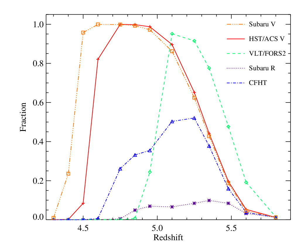
While noting all the points above, in figures 14 and 16 we illustrate in basic terms the completeness and contamination of samples derived from the selection criteria in table 1. Figure 14 shows the fraction of all galaxies (integrated to infinite faintness) detectable as a function of limiting magnitude at three different redshifts and for each selection function. As in section 2, we use the luminosity function of Lyman break galaxies (Steidel et al. 1999) for reference, while noting that changes to the shape of the luminosity function make little difference to the comparative behaviour of the selection functions (as discussed in detail in section 2.1), but have a rather larger effect on their normalisation. As a result, the numerical values in figure 14 should be viewed as indicative rather than accurate.
In figure 15 we consider a slightly different parameter, showing instead the fraction of galaxies with a continuum magnitude measured at 1500Å (rest) of , recovered by Monte Carlo simulations to a detection limit of as measured in each filter set. Model galaxies were distributed in continuum magnitude according to the measured luminosity function and their -band magnitude and colour determined as a function of redshift and filter sets, assuming a flat rest-UV continuum. Colours and magnitudes were then perturbed by random photometric errors, assuming a typical error of 0.1 mag at the selection limit of , and the fraction of galaxies satisfying the selection criteria determined. Since each band filter is suppressed by IGM absorption to a different degree as a function of redshift, the measured -band value can differ from the continuum magnitude by several tenths of a magnitude even for a flat spectrum source. As a result continuum sources close to the faint selection limit can be lost when measured in the -band. In some cases sources below that limit can be pulled up into the selection, leading to contamination of the sample by galaxies lying at but not strictly meeting a continuum selection criterion. Comparison between surveys complete to any particular magnitude is only possible if that limit is defined by flux in a band unaffected by IGM absorption.
Hence figures 14 and 15 represent a comparison of completeness for continuum-magnitude limited surveys against an ideal (infinite depth) survey, illustrating the effect of both redshift distribution and limiting magnitude on the recovery of high redshift sources. In both cases, the relative behaviour of the different filter combinations is similar. Only the two -drop samples select galaxies at since galaxies at these redshifts are too blue to be -band dropouts. By contrast all five selection functions are, in theory, sensitive to galaxies with a flat continuum at and . At both redshifts, the VLT/FORS2 filter set and selection function of Douglas et al. 200766 6 Note: Lehnert & Bremer 2003 also used this filter set but their cut reduces completeness at while leaving it unaffected at . recovers a higher fraction of the galaxies posited by any reasonable luminosity function than do the other filter sets discussed here, with the CFHT/MegaCam standard filter responses and the Subaru -drop selection performing least well.
In figure 16 we illustrate the other side of the equation, using the luminosity function determined for red galaxies at by Willmer et al. 2006 to predict their selection efficiency by any given filter and instrument combination. In each case only selection on or , and is assumed since, as demonstrated above, any associated -band is usually too shallow to reliably eliminate a sizable fraction of these sources.
Again the VLT/FORS2 filter set performs well with low sensitivity to contaminants in both redshift ranges and . Overall, the -band selection function applied at Subaru/SuprimeCam by Ouchi et al. 2004a suffers least contamination being completely insensitive to contaminants at and only weakly sensitive to them at . Although the broad HST/ACS and -bands used by the GOODS survey (Giavalisco et al. 2004) render it more vulnerable to contaminants at intermediate redshifts, these are also easier to identify morphologically from space.


The filter combinations discussed here most vulnerable to contamination by intermediate redshift galaxies are the filter sets commonly used by Subaru/SuprimeCam and CFHT/Megacam. These samples are also those most susceptible to stellar contamination as discussed in section 3.1. In both cases, the relatively short central wavelengths of the filters requires that selection colours are less extreme, and therefore admit a larger contaminant population than in other filter sets.
With the increasing availability of sensitive large format imagers, combining optical filters from multiple facilities may yield advantages in terms of tuning the redshift selection and required depth in complimentary filters.
In designing any large Lyman break galaxy survey for galaxies at it is also important to note that the best indicator of both contamination and completeness would be a spectroscopic survey reaching sensitive limits and including a large fraction of the candidate sources. Without such spectroscopy, the properties of a survey can only be modelled rather than measured.
4.2 Interpretation of the Existing Literature
Taking into account the detailed consequences of the contamination, selection and completeness issues above inevitably has consequences for the interpretation of results published and discussed in the literature. As case studies we consider three results that have attracted attention both from other observers and from theorists, and put them in the context of the labyrinthine selection function of Lyman break galaxies.
The blue rest-UV colours of Lyman break galaxies at high redshift has already been the subject of speculation and interpretation. While Lyman break dropout galaxies are largely consistent with young starbursts, their rest-UV slopes have generated comment are in many cases too blue to fit with standard population synthesis models (Yan et al. 2005; Stanway, McMahon, & Bunker 2005, e.g.). Analysing a sample of galaxies from the Hubble Ultra Deep Field, Yan et al. 2005 suggested that either a top-heavy initial mass function (IMF) or a lower than predicted intergalactic medium absorption at high redshifts could explain this result. While most of their galaxies have not been confirmed spectroscopically, at least two of the galaxies described as unusually blue have independent spectroscopy (Rhoads et al. 2005; Stanway et al. 2004) and well-detected Lyman-alpha emission lines. Taking Yan et al. 2005 object #15ab as an example, the source is known to have an emission line with =70Å at . Given this, and the effect on colour illustrated in figure 5, its colours (, ) are completely consistent with those of a flat spectrum source. Combining such an interpretation with the distribution of high equivalent widths observed in spectroscopy of the Hubble Ultra Deep Field (Stanway et al. 2007), it is not unreasonable to assume that most or all of the blue sources in this field have Lyman- emission lines (with equivalent widths explainable by standard IMFs) pointing to a young population with sporadic bursts of intense star formation (Verma et al. 2007, see also).
Accurate measurements of the rest-frame ultraviolet luminosity function of are crucial to interpreting the role of the population in cosmological processes such as the reionisation of the universe and mass build-up of the largest present day galaxies (given assumptions for the IMF and population age). Determination of the luminosity function is limited by three key parameters: the area of the survey, the depth in comparison to the typical luminosity L* and the degree to which the photometric sample represents the underlying population. Despite these limitations, estimated luminosity functions have already been used by theorists to constrain both of these processes (Mao et al. 2007; Night et al. 2006, e.g.).
Two separate luminosity functions have been derived from photometric selections, both observed from the ground using the SuprimeCam instrument, but based on different imaging filters and selection criteria. Yoshida et al. 2006 conducted their analysis on the Subaru Deep Field using the and criteria described in table 1. By contrast, Iwata et al. 2007 based their survey on a sample of a similar size, combining the Hubble Deep Field North and a second non-contiguous blank field, and substituted the filter for the used by the Subaru Deep Field team. This filter lies redwards of the and hence sources show bluer colours in the Iwata et al. 2007 sample than the Subaru Deep Field sample, while having similar colours77 7 Note: The colour-colour plots in Yoshida et al. 2006 and other Subaru Deep Field papers appear to show a systematic offset in with respect to those of other surveys, although this offset is applied uniformly to data, models and selection criteria.
In Ouchi et al. 2004b, the Subaru Deep Field team estimate the fraction of low redshift galaxy contaminants in their sample as 26% based on simulations of photometric redshift catalogues. This fraction is in good agreement with our estimate of the galactic contamination. Stellar contamination is not a serious problem for -drop surveys since cool stars are generally too red in to be confused with high redshift galaxies. Hence the galaxies are representative of the total sample contamination. By contrast, working with the same dataset, Yoshida et al. 2006 estimate their contamination as only a few percent suggesting that a degree of uncertainty exists concerning the properties of the sample.
Furthermore, the Subaru Deep Field sample is supplemented by the the sample which comprises 30 per cent of the total. As discussed in sections 3.1 and 3.2, contamination is likely to be a serious issue in the selection of Yoshida et al. 2006, with known contaminant populations conceivably accounting for all of the detected sources, and certainly accounting for %. Overall, as much as half the total sample might be accounted for by contaminants.
By contrast, the Iwata et al. 2007 survey may be comparatively clean. A bluewards shift in the near-vertical , colour track compared to the Subaru Deep Field filters has the effect of increasing the separation between the colours of model high redshift galaxies and those of most intermediate redshift interlopers. Nonetheless, some contaminant fraction is likely to remain. The scatter in optical SEDs of intermediate redshift dropout galaxies (almost four magnitudes in , as illustrated in figure 13) suggests that a spread in colours of approximately one magnitude would not be unreasonable. Given that the separation between model high and low redshift tracks is as small as 0.3 magnitudes at (and in the absence of shorter wavelength imaging), low redshift contamination is inevitable and will be biased towards the low redshift end of the sample which dominates the total number counts, particularly at bright magnitudes. Given the relative redshift range over which the two -drop samples here are susceptible to low redshift contamination, we estimate the contamination of the Iwata et al. 2007 sample as 5-10%.
The selection functions of the two surveys, which theoretically probe similar redshift ranges, clearly have massive consequences for the contamination fraction in their surveys. The distribution on those contaminants - biased to bright magnitudes in the Iwata et al. 2007 survey and peaking in the fainter sample of Yoshida et al. 2006 may go some way to explaining the differences between their derived luminosity functions. The function measured by the SDF team is steeper, finding fewer galaxies than Iwata et al. 2007 at bright magnitudes, while finding higher surface densities at faint magnitudes. Contaminants are unlikely to explain all the difference between the two luminosity functions, but certainly constitute a contributing factor which must be carefully accounted for as a function of magnitude and redshift. As a result, it is likely that neither the relatively shallow luminosity function slope of (Iwata et al. 2007) or a steeper to -2.3 (Yoshida et al. 2006) accurately describes the population at .
Although modelling is shaped by observation, rather than the reverse, comparisons between observed photometric samples and numerical models support the possibility of higher than supposed contamination in the Subaru Deep Field Sample. Kitzbichler & White 2007 used the large Millennium Simulation as the test bed for models of galaxy formation. Although these models provided a good fit to galaxy number counts at bright magnitudes and moderate redshifts, they predicted a factor of 2-8 times fewer galaxies at than observed in the SDF photometric sample.
Since the population faint end slope is essential for calculating the ionising flux contribution of the population, the same contamination issue may explain the discrepancy between the ultraviolet flux density determined from the Subaru Deep Field (Ouchi et al. 2004a) and other determinations at the same redshift (Lehnert & Bremer 2003). While the latter, based in part on a spectroscopic survey, found evidence for a decline in the ultraviolet luminosity density between and 88 8 Also seen at z=6 (Bunker et al. 2004, e.g.), Ouchi et al. 2004a found that the luminosity density shows no evidence for such a decline. Given this uncertainty, reionisation theorists should be wary of accepting the results of any one survey or selection criterion as representative of the starforming population at these redshifts.

The third key result derived from Lyman break surveys, and used to constrain high redshift galaxy models and derive the galaxy-halo bias at , is on the clustering of high redshift dropout galaxies.
The angular two-point correlation function describes the overdensity of galaxies as a function of angular scale when compared with a randomly generated distribution with the same geometry99 9 And is defined as =(GG()-2GR()+RR())/RR() where GG is the number of galaxy-galaxy pairs at a given separation, RR is the equivalent number for randomly placed galaxies and GR is the number of galaxy-random pairs (Landy & Szalay 1993).. This purely observational function yields an angular dependence and clustering amplitude such that . These can be converted into a derived clustering length given assumptions about the redshift distribution of the sample.
Measurements of the clustering at have been made based on dropout galaxies in the GOODS data and in the Subaru Deep Field. Lee et al. 2006 have explored the clustering of Lyman-Break galaxies in the GOODS fields, using the same HST/ACS filters but a slightly different selection function to that given in table 1. This survey is one of relatively few to benefit from high resolution imaging data, allowing sources of stellar morphology to be removed before analysis. The selection criteria applied in the vs colour-colour plane (a slight modification of the HST/ACS criteria used elsewhere in this paper) should successfully remove virtually all lower redshift interlopers (a fact supported by visual inspection of the candidates). However, it is not clear that the and limits (just two magnitudes deeper than ) are sufficient to support such a clean selection at the faint end of the sample. To cleanly select galaxies at (the upper end of their redshift selection) would require a -band limit some three magnitudes deeper than . Since it is not clear from Lee et al. 2006 whether non-detections in are required to satisfy the criterion or merely be consistent with it, it is possible that the sample is seriously contaminated with low redshift galaxies in the range .
The cost of this relatively clean selection (at least at bright magnitudes) is paid in allowing for relatively little scatter in the high redshift galaxy colours. Hence this result should be robust against any significant contamination from lower redshift sources but may suffer from incompleteness, particularly due to line emission towards the low redshift end of the selection. Stark et al. 2007 assess the Lee et al. 2006 sample1010 10 and the Giavalisco et al. 2004 sample on which it is based and find evidence for considerable incompleteness toward the low redshift end of their theoretical redshift selection window based on the omission of 12 out of 29 sources with spectroscopic redshifts in this range due to somewhat blue colours. The photometric selection completeness may well be better than this suggests since spectroscopic surveys are at present themselves biased towards the selection of line emitters in order to obtain a precise redshift.
Despite this latter caveat, by excluding Galactic stars the analysis of clustering at from space-based data may well be the most robust measurement available, given a sensible magnitude limit, albeit one limited to small spatial scales and understanding of their true redshift sensitivity range. The resulting measurement of correlation amplitude from Lee et al. 2006 is slightly higher than that determined at from the SDF to the same magnitude limit, but consistent within the stated errors, and also found that the best fit required a steep angular dependence, .
Ouchi et al. 2004b determined from the SDF and samples discussed above1111 11 We note that Kashikawa et al. 2006 repeated this analysis, supplementing it with slightly deeper and simulation data and determining a clustering amplitude consistent with that of Ouchi et al. 2004b.. While fixing the power law slope at , they found evidence for a larger clustering amplitude at than observed at and below, but slightly lower than that observed by Lee et al. 2006. However, as discussed earlier, a contamination fraction of 26% is estimated by the authors, and may well be much higher if the colour distribution of galaxies and cool stars are taken into account.
In both Lee et al. 2006 and Ouchi et al. 2004b, the authors make an adjustment for contaminant galaxies, but in doing so assume that such contaminants arise from photometric scatter and hence are distributed randomly in redshift and hence randomly across the sky (i.e. are unclustered). Stellar contaminants satisfying dropout criteria are indeed unlikely to be significantly correlated on the sky, although Stanway et al. 2007b did find substantial variation from field to field. By contrast, the galaxy population discussed in section 3.2 is known to be highly clustered with red galaxies more biased than blue sources at the same redshift (Coil et al. 2007). As a result, the clustering signal in a sample may be strengthened rather than weakened by the presence of contaminants.
In figure 17 we explore the effects of a small contaminant population on the clustering signal of an otherwise random galaxy distribution. We use as a base the spectroscopically confirmed dropout galaxies detected at by the DEEP2 survey. These were added to a randomly placed sample distribution of galaxies such that they comprised a varying fraction of the total sources, and the resultant clustering function was measured. As expected, the clustering amplitude declines as the fraction of randomly placed sources increases. However, as figure 17 illustrates, a contamination rate as low as 15% in an otherwise unclustered sample can produce a measurable clustering signal.
In section 3.2 we calculated that approximately 25% of the Subaru Deep Field sample is likely to lie at . Given the highly clustered nature of these contaminants, the measured angular correlation function is consistent with no clustering at all in the target population. Similarly the Lee et al. 2006 clustering result is consistent with no clustering at if just 15% of their sample lies at , and could have been attained within one standard deviation if just a few percent of their sample lies at (possible given that the numbercounts are dominated by faint source with non-detections in ).
This result does not prove that the population at is unclustered (which would be very surprising given their evident placement in massive dark matter halos), but does highlight the fact that extreme care must be taken in disentangling the influence of highly clustered contaminant populations contributing even a few percent to the total. Also interesting is that the DEEP2 data is too shallow to constrain the upturn in clustering seen at small scales by surveys and well detected by Ouchi et al. 2004b at . A simple visual inspection of high redshift candidates in Hubble Space Telescope imaging confirms that many of them form groups with multiple neighbours on the scale of a few arcseconds or less. This small scale clustering is not seen at and suggests a high galaxy-halo bias.
4.3 Implications for Higher Redshifts
In this paper we have focused on implications for galaxy surveys at since this is the largest and most-widely studied regime beyond the more easily accessible and well-known Lyman-break galaxy population at . However, the same effects as those discussed above are applicable to galaxy surveys targeted at higher redshifts.
The effects of completeness-related issues are likely to become more severe at high redshift, due to the high background in ground-based near-infrared imaging. This arises primarily from atmospheric OH emission in the and bands, and can vary dramatically on a timescale of hours. As a result, sources at certain redshifts may never be observed in Lyman- emission from the ground due to atmospheric line blanketing. The resulting broad filters, and gaps between filters, in the near infrared lead to less precise redshift discrimination, and hence potentially increased sensitivity to filter effects. While the common usage of the Mauna Kea filter set (Simons & Tokunaga 2002) is likely to mitigate this effect, where alternate filter definitions exist in the near-infrared they tend to differ dramatically in transmission profile.
In the short term, sources identified and confirmed at very high redshifts are likely to represent only those sources with high equivalent widths in Lyman- and hence may not be representative of (or, in some cases, represented in) the Lyman-break galaxy surveys that will follow.
-drop surveys, aimed at finding Lyman-break galaxies at , are susceptible to the presence of late-M , L and T stars as shown in figure 9, while near-infrared dropout samples aimed at still-higher redshift may suffer contamination from cool, red star species such as N-type carbon stars (Hawthorn et al. 2007; Totten, Irwin, & Whitelock 2000).
Just as the redshift of Lyman-break galaxies increases as longer wavelength filters are used for selection, so too does the redshift of contaminant galaxies selected for their Balmer breaks. The conventional and well studied ERO population (Simpson et al. 2006; Brown et al. 2005; Gilbank et al. 2003; Cimatti et al. 2002, e.g.) contributes contaminants to -drop samples, while the still-redder sources of Yan et al. 2004 or the population discussed by Dunlop, Cirasuolo, & McLure 2007 contribute contaminants to near-infrared dropout samples at .
Although the surface density of contaminant populations decreases as the selection moves redwards, the surface density of target high redshift galaxies also declines sharply with increasing luminosity distance. Hence an analogous situation to that at exists at higher redshifts, and the issues discussed in this paper will remain crucial to interpretations of these populations. Spectroscopy to considerable depths will almost certainly be required to characterise the properties of any high redshift sample. Given that such studies form a core component of the scientific rationale for forthcoming instruments and facilities, a firm grasp of subtle contamination and completeness issues, and a clear reporting of the methodology underlying any sample will be essential for some time to come.
5 Conclusions
The main conclusions of this paper can be summarised as follows:
(i) The redshift distribution and number counts predicted for a given survey is a sensitive function of filter profile, complicating comparisons of surface density between surveys.
(ii) Moderate line emission is sufficient to move galaxies into and out of selection functions, and can lead to scatter from the continuum galaxy locus of more than a magnitude in colour for line widths of Å. Again, the scale of this effect depends sensitively on the filter profiles.
(iii) Results derived from ultraviolet-dropout samples apply only to a subset of the total galaxy population. Quiescent galaxies - both young and old - are likely to be missed by dropout samples due to faint ultraviolet continua. Dusty galaxies at , however, are less likely to be omitted from samples than those at due to evolution in the extinction curve.
(iv) Stellar contamination can be a serious issue for dropout selections based on ground-based optical surveys. Again this effect is filter dependent, but comparison with space-based data suggests that up to 30% of some published samples might be accounted for by stellar contamination alone. In these cases infrared data may help identify contaminants.
(v) Contamination from galaxies at intermediate redshifts is again sensitive to the filters used for colour selection. A large fraction (63%) of dropout galaxies at can have , making them difficult or impossible to eliminate through optical imaging alone. The surface density of such extreme interlopers is of the same order of magnitude as the target galaxies.
(vi) The redshift range of a survey and its susceptibility to contamination can both be tuned by selecting different filter combinations, ideally selecting square-sided transmission profile filters. Deep imaging both blue and redwards of the break colours are essential to minimise contamination.
(vii) Some contaminants, with extreme colours in all bands are only ever likely to be identified spectroscopically. The deep imaging required to do so photometrically is currently infeasible bluewards of the break, and pushing the bounds of possibility in the infrared.
(viii) Care must be taken to consider selection functions and contamination fractions when interpreting and comparing the results of dropout surveys. Such effects may explain the discrepancies between results at the same redshift based on different observational data.
(ix) The clustering strength seen in surveys is entirely consistent with that expected given a small, highly-clustered contaminant population in an otherwise uncorrelated population. While this does not imply that galaxies are unclustered, it does cast doubt on the reliability of current clustering measurements.
(x) The issues discussed in this paper will remain relevant at higher redshifts, although the populations concerned and appropriate surface densities evolve with redshift.
Acknowledgements
ERS gratefully acknowledges support from the UK Science and Technology Facilities Council (STFC). We thank the DEEP2 team for making their extensive spectroscopic survey at publically available.
References
- Ajiki et al. (2006) Ajiki M., Mobasher B., Taniguchi Y., Shioya Y., Nagao T., Murayama T., Sasaki S. S., 2006, ApJ, 638, 596
- Allard & Hauschildt (1995) Allard F., Hauschildt P. H., 1995, ApJ, 445, 433
- Beckwith et al. (2006) Beckwith S. V. W., et al., 2006, AJ, 132, 1729
- Bouché, Lehnert, & Péroux (2006) Bouché N., Lehnert M. D., Péroux C., 2006, MNRAS, 367, L16
- Bouwens, Broadhurst, & Illingworth (2003) Bouwens R., Broadhurst T., Illingworth G., 2003, ApJ, 593, 640
- Bouwens et al. (2006) Bouwens R. J., Illingworth G. D., Blakeslee J. P., Franx M., 2006, ApJ, 653, 53
- Bremer et al. (2004) Bremer M. N., Lehnert M. D., Waddington I., Hardcastle M. J., Boyce P. J., Phillipps S., 2004, MNRAS, 347, L7
- Brown et al. (2005) Brown M. J. I., Jannuzi B. T., Dey A., Tiede G. P., 2005, ApJ, 621, 41
- Bruzual & Charlot (2003) Bruzual G., Charlot S., 2003, MNRAS, 344, 1000
- Bruzual (2007) Bruzual A G., 2007, arXiv:astro-ph/0702091, Proceedings of the Meeting ”From Stars to Galaxies: Building the Pieces to Build Up the Universe”, eds. A. Vallenari, R. Tantalo, L. Portinari, and A. Moretti, ASP Conf. Ser. (in press)
- Bunker et al. (2004) Bunker A. J., Stanway E. R., Ellis R. S., McMahon R. G., 2004, MNRAS, 355, 374
- Chary et al. (2007) Chary R.-R., Teplitz H. I., Dickinson M. E., Koo D. C., Le Floc’h E., Marcillac D., Papovich C., Stern D., 2007, ApJ, 665, 257
- Cimatti et al. (2002) Cimatti A., et al., 2002, A&A, 381, L68
- Coil et al. (2007) Coil A. L., Hennawi J. F., Newman J. A., Cooper M. C., Davis M., 2007, ApJ, 654, 115
- Condon, Balonek, & Jauncey (1975) Condon J. J., Balonek T. J., Jauncey D. L., 1975, AJ, 80, 887
- Davis et al. (2003) Davis M., et al., 2003, SPIE, 4834, 161
- Douglas et al. (2007) Douglas L. S., Bremer M. N., Stanway E. R., Lehnert M. D., 2007, MNRAS, 376, 1393
- Dunlop, Cirasuolo, & McLure (2007) Dunlop J. S., Cirasuolo M., McLure R. J., 2007, MNRAS, 376, 1054
- Eyles et al. (2005) Eyles L. P., Bunker A. J., Stanway E. R., Lacy M., Ellis R. S., Doherty M., 2005, MNRAS, 364, 443
- Franx et al. (2003) Franx M., et al., 2003, ApJ, 587, L79
- Giavalisco et al. (2004) Giavalisco M., et al., 2004, ApJ, 600, L93
- Giavalisco et al. (2004) Giavalisco M., et al., 2004, ApJ, 600, L103
- Gilbank et al. (2003) Gilbank D. G., Smail I., Ivison R. J., Packham C., 2003, MNRAS, 346, 1125
- Hawley et al. (2002) Hawley S. L., et al., 2002, AJ, 123, 3409
- Hawthorn et al. (2007) Hawthorn, M. J. et al., 2007, in preparation
- Hayes & Östlin (2006) Hayes M., Östlin G., 2006, A&A, 460, 681
- Hu et al. (2004) Hu E. M., Cowie L. L., Capak P., McMahon R. G., Hayashino T., Komiyama Y., 2004, AJ, 127, 563
- Iwata et al. (2007) Iwata I., Ohta K., Tamura N., Akiyama M., Aoki K., Ando M., Kiuchi G., Sawicki M., 2007, MNRAS, 376, 1557
- Kashikawa et al. (2004) Kashikawa N., et al., 2004, PASJ, 56, 1011
- Kashikawa et al. (2006) Kashikawa N., et al., 2006, ApJ, 637, 631
- Kitzbichler & White (2007) Kitzbichler M. G., White S. D. M., 2007, MNRAS, 376, 2
- Knapp et al. (2004) Knapp G. R., et al., 2004, AJ, 127, 3553
- Knudsen et al. (2005) Knudsen K. K., et al., 2005, ApJ, 632, L9
- Labbé et al. (2005) Labbé I., et al., 2005, ApJ, 624, L81
- Landy & Szalay (1993) Landy S. D., Szalay A. S., 1993, ApJ, 412, 64
- Lee et al. (2006) Lee K.-S., Giavalisco M., Gnedin O. Y., Somerville R. S., Ferguson H. C., Dickinson M., Ouchi M., 2006, ApJ, 642, 63
- Lehnert & Bremer (2003) Lehnert M. D., Bremer M., 2003, ApJ, 593, 630
- Leitherer et al. (1999) Leitherer C., et al., 1999, ApJS, 123, 3
- Madau (1995) Madau P., 1995, ApJ, 441, 18
- Madau et al. (1996) Madau P., Ferguson H. C., Dickinson M. E., Giavalisco M., Steidel C. C., Fruchter A., 1996, MNRAS, 283, 1388
- Maiolino et al. (2004) Maiolino R., Schneider R., Oliva E., Bianchi S., Ferrara A., Mannucci F., Pedani M., Roca Sogorb M., 2004, Nature, 431, 533
- Malhotra & Rhoads (2004) Malhotra S., Rhoads J. E., 2004, ApJ, 617, L5
- Mao et al. (2007) Mao J., Lapi A., Granato G. L., de Zotti G., Danese L., 2007, ApJ, 667, 655
- Maraston (2005) Maraston C., 2005, MNRAS, 362, 799
- Marchesini et al. (2007) Marchesini D., et al., 2007, ApJ, 656, 42
- McLure et al. (2006) McLure R. J., et al., 2006, MNRAS, 372, 357
- Mobasher et al. (2005) Mobasher B., et al., 2005, ApJ, 635, 832
- Night et al. (2006) Night C., Nagamine K., Springel V., Hernquist L., 2006, MNRAS, 366, 705
- Oke & Gunn (1983) Oke J. B., Gunn J. E., 1983, ApJ, 266, 713
- Ouchi et al. (2004a) Ouchi M., et al., 2004a, ApJ, 611, 660
- Ouchi et al. (2004b) Ouchi M., et al., 2004b, ApJ, 611, 685
- Patten et al. (2006) Patten B. M., et al., 2006, ApJ, 651, 502
- Pentericci et al. (2007) Pentericci L., Grazian A., Fontana A., Salimbeni S., Santini P., de Santis C., Gallozzi S., Giallongo E., 2007, A&A, 471, 433
- Rhoads et al. (2005) Rhoads J. E., et al., 2005, ApJ, 621, 582
- Rodighiero et al. (2007) Rodighiero G., Cimatti A., Franceschini A., Brusa M., Fritz J., Bolzonella M., 2007, A&A, 470, 21
- Shapley et al. (2003) Shapley A. E., Steidel C. C., Pettini M., Adelberger K. L., 2003, ApJ, 588, 65
- Simons & Tokunaga (2002) Simons D. A., Tokunaga A., 2002, PASP, 114, 169
- Simpson et al. (2006) Simpson C., et al., 2006, MNRAS, 373, L21
- Stanway, Bunker, & McMahon (2003) Stanway E. R., Bunker A. J., McMahon R. G., 2003, MNRAS, 342, 439
- Stanway et al. (2004) Stanway E. R., Bunker A. J., McMahon R. G., Ellis R. S., Treu T., McCarthy P. J., 2004, ApJ, 607, 704
- Stanway, McMahon, & Bunker (2005) Stanway E. R., McMahon R. G., Bunker A. J., 2005, MNRAS, 359, 1184
- Stanway et al. (2007) Stanway E. R., et al., 2007, MNRAS, 376, 727
- Stanway et al. (2007b) Stanway E. R., Bremer M. N., Lehnert M. D., Eldridge J. J., 2007, arXiv, 711, arXiv:0711.2457
- Stark et al. (2007) Stark D. P., Bunker A. J., Ellis R. S., Eyles L. P., Lacy M., 2007, ApJ, 659, 84
- Steidel et al. (1999) Steidel C. C., Adelberger K. L., Giavalisco M., Dickinson M., Pettini M., 1999, ApJ, 519, 1
- Stratta et al. (2007) Stratta G., Maiolino R., Fiore F., D’Elia V., 2007, ApJ, 661, L9
- Thomas et al. (2005) Thomas D., Maraston C., Bender R., Mendes de Oliveira C., 2005, ApJ, 621, 673
- Totten, Irwin, & Whitelock (2000) Totten E. J., Irwin M. J., Whitelock P. A., 2000, MNRAS, 314, 630
- Vanzella et al. (2006) Vanzella E., et al., 2006, A&A, 454, 423
- Verma et al. (2007) Verma A., Lehnert M. D., Förster Schreiber N. M., Bremer M. N., Douglas L., 2007, MNRAS, 294
- Willmer et al. (2006) Willmer C. N. A., et al., 2006, ApJ, 647, 853
- Yan et al. (2004) Yan H., et al., 2004, ApJ, 616, 63
- Yan et al. (2005) Yan H., et al., 2005, ApJ, 634, 109
- Yoshida et al. (2006) Yoshida M., et al., 2006, ApJ, 653, 988