Virtual Bridge Number One Knots

Evarist Byberi and Vladimir V. Chernov (Tchernov) Address: E. Byberi, HB 0552 Dartmouth College, Hanover NH 03755, USA Email address: Evarist.Byberi@dartmouth.edu Address: V. Chernov, Department of Mathematics, 6188 Bradley Hall, Dartmouth College, Hanover NH 03755, USA Email address: Vladimir.Chernov@dartmouth.edu

Abstract.

We define the virtual bridge number $\operatorname{vb}(K)$ and the virtual unknotting number $\operatorname{vu}(K)$ invariants for virtual knots. For ordinary knots $K$ they are closely related to the bridge number $b(K)$ and the unknotting number $u(K)$ and we have $\operatorname{vu}(K)\leq u(K),\operatorname{vb}(K)\leq b(K).$

There are no ordinary knots $K$ with $b(K)=1.$ We show there are infinitely many homotopy classes of virtual knots each of which contains infinitely many isotopy classes of $K$ with $\operatorname{vb}(K)=1.$ In fact for each $i\in{\mathbb{N}}$ there exists $K$ virtually homotopic (but not virtually isotopic) to the unknot with $\operatorname{vb}(K)=1$ and $\operatorname{vu}(K)=i.$

Key words and phrases:

unknotting number, bridge number, virtual knot, virtual string

1991 Mathematics Subject Classification

Primary 57M25; Secondary 57M27

1. Introduction into Virtual Knots

The Virtual Knot Theory was introduced by L. Kauffman [5]. Let us recall some of its basic notions.

A knot is a smooth embedding $S^{1}\to{\mathbb{R}}^{3}$ . It can be described by its knot diagram which is a generic immersion of $S^{1}$ into the ${\mathbb{R}}^{2}$ -plane equipped with information about over-passes and under-passes at double points. A knot diagram $D$ gives rise to a Gauss diagram $G_{D}$ that is a circle parameterizing the knot with each pair of preimages of double points of $D$ connected by an oriented signed chord. The chords are oriented from the preimage point on the over-passing branch to the preimage point on the under-passing branch. The sign of a chord is the sign of the corresponding double point. The resulting Gauss diagram $G_{D}$ is called the Gauss diagram of the knot diagram $D$ .

Refer to caption — Figure 1. A knot diagram and the corresponding Gauss diagram

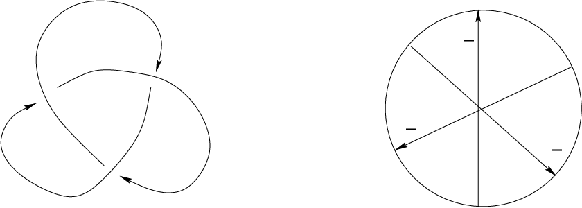
Gauss diagrams that are obtainable as Gauss diagrams of some knot diagrams are said to be realizable. A knot diagram corresponding to a realizable Gauss diagram can be recovered only up to a certain ambiguity. However the isotopy type of the corresponding knot is recoverable in a unique way.

It is well-known that two knots described by their knot diagrams are isotopic if and only if one can change one diagram to another by a sequence of ambient isotopies of the diagram and of Reidemeister moves shown in Figure 2.

The Redemeister moves can be easily encoded [1] in the language of Gauss diagrams, see Figure 3. The equivalence classes of the, not necessarily realizable, Gauss diagrams modulo the resulting moves are called virtual knots.

2. Main results

2.1 Definition (virtual bridge number).

Recall that a bridge in a knot diagram is an arc between two consecutive underpasses that contains nonzero many overpasses. The bridge number $b(K)$ of a knot $K$ , is the minimum number of bridges in a knot diagram realizing $K.$ Given a Gauss diagram constructed from a knot diagram, the number of bridges in it is the number of circle arcs between two consecutive arrow heads that contain nonzero many arrow ends. Note that this number is well defined even for nonrealizable Gauss diagrams, and we call it the number of bridges in a Gauss diagram. The virtual bridge number $\operatorname{vb}(K)$ of a virtual knot $K$ is the minimum number of bridges over all the Gauss diagrams realizing $K.$ If $\operatorname{vb}(K)=0,$ then $K$ is the unknot. Note that if $K$ is isotopic to an ordinary knot then $\operatorname{vb}(K)\leq b(K).$ It is plausible that for many $K$ we should actually have $\operatorname{vb}(K)=b(K),$ but we have not studied this question yet.

2.2 Definition.

An isotopy between two Gauss diagrams is a sequence of the Gauss diagram versions of Reidemeister moves.

2.3 Definition.

A (generic) homotopy between two Gauss diagrams is a sequence of isotopies and “flip moves” that change simultaneously the direction and the sign of an arrow. If a Gauss diagram corresponds to a knot diagram, then the last move reflects the passage of a knot through a singular double point at a crossing identified with the arrow.

Note that any two knots in ${\mathbb{R}}^{3}$ are homotopic as loops. However there are many different homotopy classes of virtual knots. In particular not every virtual knot is homotopic to the unknot.

2.4 Definition.

For an ordinary knot $K$ , its unknotting number $u(K)$ is the minimal number of passages through a double point of two branches of the knot in a generic homotopy of $K$ to the unknot.

For virtual knots, the unknot is the trivial Gauss diagram with no chords. If $K$ is a virtual knot homotopic to the unknot, then we put the virtual unknotting number $\operatorname{vu}(K)$ to be the minimal number of flip moves in a virtual homotopy that changes $K$ to the unknot. Note that if $K$ is nontrivial, then $\operatorname{vu}(K)\geq 1.$

Clearly if $K$ is an ordinary knot, then $\operatorname{vu}(K)\leq u(K).$ For many knots we have $\operatorname{vu}(K)=u(K).$ For example this is always true if $u(K)=1.$

Let $K_{1},K_{2}$ be two different virtual knots that are homotopic to each other. We put the relative unknotting number $\operatorname{rvu}(K_{1},K_{2})$ to be the minimal number of flip moves in a generic homotopy of $K_{1}$ to $K_{2}.$ Clearly if $K_{1},K_{2}$ are homotopic to the unknot, then we have $\operatorname{rvu}(K_{1},K_{2})\leq\operatorname{vu}(K_{1})+\operatorname{vu}(K_{2}).$ Moreover if $K_{2}$ is the unknot, then $\operatorname{rvu}(K_{1},K_{2})=\operatorname{vu}(K_{1}).$

It is well-known that there are no ordinary knots $K$ with $b(K)=1.$ However, as we show, the theory of virtual knots with $\operatorname{vb}(K)=1$ is surprisingly nontrivial.

2.5 Theorem.

For every $i\in{\mathbb{N}}$ there exists a virtual knot $K_{i}$ homotopic to the unknot that has $\operatorname{vb}(K_{i})=1$ and $\operatorname{vu}(K_{i})=i.$

The following Theorem can be thought of a generalization of the above result to the case of virtual knots that are not homotopic to the unknot.

2.6 Theorem.

There are infinitely many virtual knot homotopy classes $H^{p,q}$ enumerated by pairs of distinct positive integers $(p,q)$ such that $H^{p,q}$ contains infinitely many distinct virtual knots $\{K^{p,q}_{j}\}_{j=0}^{\infty}$ with $\operatorname{vb}(K^{p,q}_{j})=1$ and $\operatorname{rvu}(K^{p,q}_{j_{1}},K^{p,q}_{j_{2}})=|j_{1}-j_{2}|$ for all $j_{1},j_{2}.$

Note that for a virtual knot homotopy class not containing the unknot, there is no obvious choice of the most trivial knot in the class. In the examples constructed in the proof of Theorem 2.6 the knots $K^{p,q}_{0}$ are simpler than all $K^{p,q}_{j},j\geq 1.$ So one can think of them as the chosen most trivial knots in the corresponding virtual homotopy classes.

3. Proofs

In the proofs of Theorems 2.5 and 2.6 we use properties of invariants studied by V. Turaev [6, 7] and A. Henrich [4].

3.1. Invariants of V. Turaev and A. Henrich

3.1 Definition (Invariant $P(K)$ of A. Henrich [4]).

Let $D$ be a Gauss diagram realizing a virtual knot $K.$ The end points of a chord $c$ in $D$ separate the circle in $D$ into two arcs. Choose one of the arcs and perform the flip moves on all the other chords so that they point into the chosen arc. Let $i(c)$ to be the sum of the signs $\pm 1$ of the chords pointing into the chosen arc after the flip moves. We put $\operatorname{sign}(c)=\pm 1$ to be the sign of $c.$

Put

(3.1)

P(D)=\sum_{c\text{ such that }i(c)\neq 0}\operatorname{sign}(c)t^{|i(c)|}

to be the polynomial in variable $t$ with integer coefficients. One can show that $P(D)$ does not depend on the choice of the diagram $D$ realizing $K$ . Hence we have a polynomial invariant $P(K)$ of a virtual knot $K.$ It is easy to see that $P$ is a Vassiliev-Goussarov invariant [8], [2], [3] of order one of virtual knots in the sense of Kauffman [5]¹¹ 1 Note that Goussarov, Polyak and Viro [1] used a different notion of finite order invariants of virtual knots and our invariant is not of order one in the sense of their work..

This invariant, in a slightly different form, was introduced by A. Henrich [4]. It is also related to the cobordism invariants of knots in thickened surfaces studied by V. Turaev [7].

3.2 Remark (The $P$ invariant and the virtual unknotting numbers $\operatorname{rvu},\operatorname{vu}$ ).

It is easy to see that a flip move on a chord $c$ with $i(c)\neq 0$ changes one of the coefficients of the polynomial $P$ invariant by $2$ . The flip move on a chord $c$ with $i(c)=0$ does not change the $P$ invariant. Thus, as it was observed by A. Henrich [4], if $K_{1},K_{2}$ are homotopic virtual knots and $P(K_{1})-P(K_{2})=\sum_{j>0}a_{j}t^{j}$ , then every (generic) homotopy between $K_{1}$ and $K_{2}$ involves at least $\frac{\sum_{j>0}|a_{j}|}{2}$ flip moves. Thus $\operatorname{rvu}(K_{1},K_{2})\geq\frac{\sum_{j>0}|a_{j}|}{2}.$

Let $K$ be a virtual knot homotopic to the trivial knot $K_{0}.$ Let $P(K)=\sum_{j>0}b_{j}t^{j}$ . Since $P(K_{0})=0,$ the above relation of the $P$ invariant with the relative unknotting number $\operatorname{rvu}$ implies that the vitual unknotting number $\operatorname{vu}(K)\geq\frac{\sum_{j>0}|b_{j}|}{2}.$

3.3 Definition ( $u$ -invariant of V. Turaev [6]).

Let $D$ be a Gauss diagram realizing a virtual knot $K.$ Let $\overline{D}$ be the Gauss diagram obtained from $D$ by performing the flip moves that convert the signs of all the chords to be $+1.$ The end points of an oriented chord $c$ separate the core circle of $\overline{D}$ into two oriented arcs. The oriented arc that starts at the arrow head of $c$ would be called the preferred arc and denoted by $A^{+}_{c}$ . The other arc is $A^{-}_{c}.$ Put $n_{+}(c)$ to be the number of oriented chords different from $c$ that start in $A^{-}_{c}$ and end in $A^{+}_{c}.$ Put $n_{-}(c)$ to be the number of oriented chords different from $c$ that start in $A^{+}_{c}$ and end in $A^{-}_{c}.$ Put $n(c)=n_{+}(c)-n_{-}(c)$ and put $\operatorname{sign}(n(c))=\pm 1$ to be the sign of $n(c).$

Put

(3.2)

u(D)=\sum_{c\in\overline{D}\text{ such that }n(c)\neq 0}\operatorname{sign}(n(c))t^{|n(c)|}

to be a polynomial in $t$ with integer coefficients. This $u(D)$ in a slightly different form was introduced by V. Turaev [6]. From his work one immediately gets that $u(D)$ depends only on the virtual homotopy class of the virtual knot $K.$ In particular, if for two virtual knots $K_{1},K_{2}$ we have $u(K_{1})\neq u(K_{2})$ , then $K_{1}$ and $K_{2}$ are not virtually homotopic.

3.2. Proof of Theorem 2.5

Consider the virtual knots $\{K_{i}\}_{i=0}^{\infty}$ depicted in Figure 4. All these knots are virtually homotopic. Indeed to get from $K_{i+1}$ to $K_{i}$ perform a flip move on the chord in $K_{i+1}$ with the rightmost arrow head. Then use the Gauss diagram version of the second Reidemeister move, see Figure 3, to cancel the resulting chord and the chord with the left most arrow head in $K_{i+1}$ . Since $K_{0}$ is the trivial knot, we see that $\operatorname{vu}(K_{i})\leq i$ for all $i\in{\mathbb{N}}.$

A straightforward computation shows that $P(K_{i})=2t^{2i-1}+2t^{2i-3}+\dots+2t^{1}.$ As it was discussed in Remark 3.2 this means that $\operatorname{vu}(K_{i})\geq\frac{2i}{2}=i.$ Hence $\operatorname{vu}(K_{i})=i.$

It is easy to see that $\operatorname{vb}(K_{i})\leq 1$ for $i\geq 1.$ Since $P(K_{i})\neq 0$ for $i\geq 1$ , these virtual knots are nontrivial and hence $\operatorname{vb}(K_{i})=1$ for all $i\geq 1.$ ∎

3.3. Proof of Theorem 2.6

For $p,q\in{\mathbb{N}}$ with $p\neq q$ we put $K_{0}^{p,q}$ to be the virtual knot shown in Figure 5 whose Gauss diagram consists of $p$ parallel positive vertical chords oriented upwards and $q$ parallel positive horizontal chords oriented to the right. A straightforward computation shows that $u(K_{0}^{p,q})=-pt^{q}+qt^{p}.$ Since $u$ is invariant under virtual homotopy we see that if $p_{1},q_{1},p_{2},q_{2}\in{\mathbb{N}}$ are such $p_{1}\neq q_{1}$ , $p_{2}\neq q_{2}$ and $(p_{1},q_{1})\neq(p_{2},q_{2})$ , then $K_{0}^{p_{1},q_{1}}$ and $K_{0}^{p_{2},q_{2}}$ are not virtually homotopic.

If we draw the horizontal and vertical arrows of $K_{0}^{p,q}$ to be close to the $x$ - and $y$ -axis, then we have four large arcs of the circle in $K^{p,q}_{0}$ that are free of chord ends. We will refer to these arcs as the arcs located in the corresponding four quadrants. For $n\in{\mathbb{N}}$ put $K_{n}^{p,q}$ to be the virtual knot whose Gauss diagram is obtained from the diagram of $K_{0}^{p,q}$ by adding $2n$ positive chords that pass through the circle center. The first $n$ of the added chords should start in the fourth quadrant arc, end in the second quadrant arc and have almost vertical slope. The other $n$ chords should start in the second quadrant arc, end in the fourth quadrant arc and have almost horizontal slope, see Figure 6.

We claim that for fixed $p,q$ all the knots $K_{n}^{p,q}$ are virtually homotopic. For $n\geq 1$ the homotopy between $K_{n}^{p,q}$ and $K_{n-1}^{p,q}$ is constructed as follows. Take the chord from the group of $n$ chords going from the second to the fourth quadrant arc whose slope is the farthest from the horizontal one and perform the flip move on it. Use the Gauss diagram version of the second Reidemiester move to cancel the resulting chord and the chord in the group of $n$ chords going from the fourth into the second quadrant arc whose slop is the farthest from the vertical, see Figure 7. Since this virtual homotopy between $K_{n}^{p,q}$ and $K_{n-1}^{p,q}$ involves only one flip move, we have $\operatorname{rvu}(K_{n_{1}}^{p,q},K_{n_{2}}^{p,q})\leq|n_{1}-n_{2}|,$ for all $n_{1},n_{2}$ .

A straightforward computation shows that

(3.3)

\begin{split}P(K_{n}^{p,q})=\\ t^{2n+p+q-1}+\dots+t^{2n+p+q-(2n-1)}+qt^{p}+pt^{q}+t^{p+q+1}+\dots t^{p+q+(2n-1)}=\\ qt^{p}+pt^{q}+\sum_{i=1}^{n}2t^{p+q+(2i-1)}.\end{split}

Thus

(3.4)

P(K_{n_{1}}^{p,q})-P(K_{n_{2}}^{p,q})=\sum_{i=\min(n_{1},n_{2})+1}^{i=\max(n_{1},n_{2})}2t^{p+q+2i-1}.

Hence by Remark 3.2, $\operatorname{rvu}(K_{n_{1}}^{p,q},K_{n_{2}}^{p,q})\geq\frac{2|n_{2}-n_{1}|}{2}=|n_{2}-n_{1}|.$ Thus we have $\operatorname{rvu}(K_{n_{1}}^{p,q},K_{n_{2}}^{p,q})=|n_{2}-n_{1}|.$

It is easy to see that $\operatorname{vb}(K^{p,q}_{n})\leq 1.$ Since $P(K^{p,q}_{n})\neq 0$ , these knots are nontrivial and we have $\operatorname{vb}(K^{p,q}_{n})=1.$ ∎.

Acknowledgments. The second author is very thankful to Alina Vdovina for the very useful mathematical discussions during which the notion of the virtual bridge number was introduced.

References

[1] M. Goussarov, M. Polyak and O. Viro: Finite-type invariants of classical and virtual knots, Topology 39 (2000), no. 5, 1045–1068.
[2] M. Goussarov, A talk on 12.1.1987 where the finite order invariants were first defined at the Rokhlin seminar at the Steklov Institute for Mathematics, St Petersburg, Russia.
[3] M. Gouusarov (Gusarov), A new form of the Conway-Jones polynomial of oriented links. (Russian. English summary) Zap. Nauchn. Sem. Leningrad. Otdel. Mat. Inst. Steklov. (LOMI) 193 (1991), Geom. i Topol. 1, 4–9, 161.
[4] A. Henrich, Ph.D. thesis, expected in Spring (2008)
[5] L. H. Kauffman: Virtual Knot Theory, European J. Comb. 20 (1999), 663-690.
[6] V. Turaev, Virtual strings. Ann. Inst. Fourier (Grenoble) 54 (2004), no. 7, 2455–2525 (2005)
[7] V. Turaev, Cobordism of knots on surfaces, preprint arXiv:math/0703055 available at http://www.arXiv.org, 28 pages (2007)
[8] V. Vassiliev, Cohomology of knot spaces, Theory of singularities and its applications, pp. 23–69, Adv. Soviet Math., 1, Amer. Math. Soc., Providence, RI, (1990)