跳到论文正文
W Papers独立论文阅读器 arXiv:0712.2258 论文正文 计算阅读时间 · 0%
引用这篇论文根据当前论文元数据生成,正式投稿前建议核对。


License: Assumed arXiv.org perpetual non-exclusive license
arXiv:0712.2258v1 [math.NA] 13 Dec 2007

Subspace correction methods for total variation and ℓ1−\ell_{1}-minimization

Massimo Fornasier Thanks: Johann Radon Institute for Computational and Applied Mathematics (RICAM), Austrian Academy of Sciences, Altenbergerstrasse 69, A-4040, Linz, Austria Email: massimo.fornasier@oeaw.ac.at    Carola-Bibiane Schönlieb Thanks: Department of Applied Mathematics and Theoretical Physics (DAMTP), Centre for Mathematical Sciences, Wilberforce Road, Cambridge CB3 0WA, United Kingdom.Email: c.b.s.schonlieb@damtp.cam.ac.uk
Abstract

This paper is concerned with the numerical minimization of energy functionals in Hilbert spaces involving convex constraints coinciding with a semi-norm for a subspace. The optimization is realized by alternating minimizations of the functional on a sequence of orthogonal subspaces. On each subspace an iterative proximity-map algorithm is implemented via oblique thresholding, which is the main new tool introduced in this work. We provide convergence conditions for the algorithm in order to compute minimizers of the target energy. Analogous results are derived for a parallel variant of the algorithm. Applications are presented in domain decomposition methods for singular elliptic PDE’s arising in total variation minimization and in accelerated sparse recovery algorithms based on ℓ1\ell_{1}-minimization. We include numerical examples which show efficient solutions to classical problems in signal and image processing.

keywords
Domain decomposition method, subspace corrections, convex optimization, parallel computation, discontinuous solutions, total variation minimization, singular elliptic PDE’s, ℓ1\ell_{1}-minimization, image and signal processing
AMS
65K10, 65N55 65N21, 65Y05 90C25, 52A41, 49M30, 49M27, 68U10

1 Introduction

Let ℋ\mathcal{H} be a real separable Hilbert space. We are interested in the numerical minimization in ℋ\mathcal{H} of the general form of functionals

𝒥⁡(u):=‖T​u−g‖ℋ2+2​α​ψ​(u),\mathcal{J}(u):=\|Tu-g\|_{\mathcal{H}}^{2}+2\alpha\psi(u),

where T∈ℒ⁡(ℋ)T\in\mathcal{L}(\mathcal{H}) is a bounded linear operator, g∈ℋg\in\mathcal{H} is a datum, and α>0\alpha>0 is a fixed constant. The function ψ:ℋ→ℝ+∪{+∞}\psi:\mathcal{H}\to\mathbb{R}_{+}\cup\{+\infty\} is a semi-norm for a suitable subspace ℋψ\mathcal{H}^{\psi} of ℋ\mathcal{H}. In particular, we investigate splittings into arbitrary orthogonal subspaces ℋ=V1⊕V2\mathcal{H}=V_{1}\oplus V_{2} for which we may have

ψ⁡(πV1​(u)+πV2​(v))≠ψ⁡(πV1​(u))+ψ⁡(πV2​(v)),u,v∈ℋ,\psi(\pi_{V_{1}}(u)+\pi_{V_{2}}(v))\neq\psi(\pi_{V_{1}}(u))+\psi(\pi_{V_{2}}(v)),\quad u,v\in\mathcal{H},

where πVi\pi_{V_{i}} is the orthogonal projection onto ViV_{i}. With this splitting we want to minimize 𝒥\mathcal{J} by suitable instances of the following alternating algorithm: Pick an initial V1⊕V2∋u1(0)+u2(0):=u(0)∈ℋΨV_{1}\oplus V_{2}\ni u_{1}^{(0)}+u_{2}^{(0)}:=u^{(0)}\in\mathcal{H}^{\Psi}, for example u(0)=0u^{(0)}=0, and iterate

{u1(n+1)≈\argminv1∈V1​𝒥​(v1+u2(n))u2(n+1)≈\argminv2∈V2​𝒥​(u1(n+1)+v2)u(n+1):=u1(n+1)+u2(n+1).\left\{\begin{array}[]{ll}u_{1}^{(n+1)}\approx\argmin_{v_{1}\in V_{1}}\mathcal{J}(v_{1}+u_{2}^{(n)})&\\ u_{2}^{(n+1)}\approx\argmin_{v_{2}\in V_{2}}\mathcal{J}(u_{1}^{(n+1)}+v_{2})&\\ u^{(n+1)}:=u_{1}^{(n+1)}+u_{2}^{(n+1)}.\end{array}\right.

This algorithm is implemented by solving the subspace minimizations via an oblique thresholding iteration. We provide a detailed analysis of the convergence properties of this sequential algorithm and of its modification for parallel computation. We motivate this rather general approach by two relevant applications in domain decomposition methods for total variation minimization and in accelerated sparse recovery algorithms based on ℓ1\ell_{1}-minimization. Nevertheless, the applicability of our results reaches far beyond these particular examples.

1.1 Domain decomposition methods for singular elliptic PDE’s

Domain decomposition methods were introduced as techniques for solving partial differential equations based on a decomposition of the spatial domain of the problem into several subdomains [33, 7, 47, 15, 36, 48, 32, 6, 34]. The initial equation restricted to the subdomains defines a sequence of new local problems. The main goal is to solve the initial equation via the solution of the local problems. This procedure induces a dimension reduction which is the major responsible of the success of such a method. Indeed, one of the principal motivations is the formulation of solvers which can be easily parallelized.
We apply the theory and the algorithms developed in this paper to adapt domain decompositions to the minimization of functionals with total variation constraints. Differently from situations classically encountered in domain decomposition methods for nonsingular PDE’s, where solutions are usually supposed at least continuous, in our case the interesting solutions may be discontinuous, e.g., along curves in 2D. These discontinuities may cross the interfaces of the domain decomposition patches. Hence, the crucial difficulty is the correct treatment of interfaces, with the preservation of crossing discontinuities and the correct matching where the solution is continuous instead. We consider the minimization of the functional 𝒥\mathcal{J} in the following setting: Let Ω⊂ℝd\Omega\subset\mathbb{R}^{d}, for d=1,2d=1,2, be a bounded open set with Lipschitz boundary. We are interested in the case when ℋ=L2​(Ω)\mathcal{H}=L^{2}(\Omega), ℋψ=B​V​(Ω)\mathcal{H}^{\psi}=BV(\Omega) and ψ⁡(u)=|D​u|(Ω)\psi(u)=|Du|(\Omega), the variation of uu. Then a domain decomposition Ω=Ω1∪Ω2\Omega=\Omega_{1}\cup\Omega_{2} induces the space splitting into Vi:={u∈L2​(Ω):supp​(u)⊂Ωi}V_{i}:=\{u\in L^{2}(\Omega):\textrm{supp}(u)\subset\Omega_{i}\}, i=1,2i=1,2. Hence, by means of the proposed alternating algorithm, we want to minimize the functional

𝒥⁡(u):=‖T​u−g‖L2​(Ω)2+2​α​|D​u|​(Ω).\mathcal{J}(u):=\|Tu-g\|_{L^{2}(\Omega)}^{2}+2\alpha|Du|(\Omega).

The minimization of energies with total variation constraints traces back to the first uses of such a functional model in noise removal in digital images as proposed by Rudin, Osher, and Fatemi [39]. There the operator TT is just the identity. Extensions to more general operators TT and numerical methods for the minimization of the functional appeared later in several important contributions [14, 22, 3, 45, 13]. From these pioneering and very successful results, the scientific output related to total variation minimization and its applications in signal and image processing increased dramatically in the last decade. It is not worth here to mention all the possible directions and contributions. We limit ourself to mention that, to our knowledge, this paper is the first in presenting a successful domain decomposition approach to total variation minimization. The motivation is that several approaches are directed to the solution of the Euler-Lagrange equations associated to the functional 𝒥\mathcal{J}, which determine a singular elliptic PDE involving the 11-Laplace operator. Due to the fact that |D​u|​(Ω)|Du|(\Omega) is not differentiable, one has to discretize its subdifferential, and its characterization is indeed hard to implement numerically in a correct way. The lack of a simple characterization of the subdifferential of the total variation especially raises significant difficulties in dealing with discontinuous interfaces between patches of a domain decomposition. Our approach overcomes these difficulties by minimizing the functional via an iterative proximity-map algorithm, as proposed, e.g., in [13], instead of attempting the direct solution of the Euler-Lagrange equations. It is also worth to mention that, due to the generality of our setting, our approach can be extended to more general subspace decompositions, not only those arising from a domain splitting. This can open room to more sophisticated multiscale algorithms where ViV_{i} are multilevel spaces, e.g., from a wavelet decomposition.

1.2 Accelerated sparse recovery algorithms based on ℓ1\ell_{1}-minimization

In this application, we are concerned with the use of the alternating algorithm to the case where Λ\Lambda is a countable index set, ℋ=ℓ2​(Λ)\mathcal{H}=\ell_{2}(\Lambda), and ψ⁡(u)=‖u‖ℓ1​(Λ):=∑λ∈Λ|uλ|\psi(u)=\|u\|_{\ell_{1}(\Lambda)}:=\sum_{\lambda\in\Lambda}|u_{\lambda}|. The minimization of the functional

𝒥⁡(u):=‖T​u−g‖ℓ2​(Λ)2+2​α​‖u‖ℓ1,\mathcal{J}(u):=\|Tu-g\|_{\ell_{2}(\Lambda)}^{2}+2\alpha\|u\|_{\ell_{1}},

proved to be an extremely efficient alternative to the well-known Tikhonov regularization [27], whenever

T​u=g,Tu=g,

is an ill-posed problem and the solution uu is expected to be a vector with a moderate number of nonzero entries. Indeed, the imposition of the ℓ1\ell_{1}-constraint does promote a sparse solution. The use of the ℓ1\ell_{1} norm as a sparsity-promoting functional can be found first in reflection seismology and in deconvolution of seismic traces [17, 40, 42]. In the last decade more understanding of the deep motivations why ℓ1\ell_{1}-minimization tends to promote sparse recovery was developed. Rigorous results began to appear in the late-1980’s, with Donoho and Stark [25] and Donoho and Logan [24]. Applications for ℓ1\ell_{1} minimization in statistical estimation began in the mid-1990’s with the introduction of the LASSO algorithm [43] (iterative thresholding). In the signal processing community, Basis Pursuit [16] was proposed in compression applications for extracting a sparse signal representation from highly overcomplete dictionaries. From these early steps the applications and understanding of ℓ1\ell_{1} minimization have continued to increase dramatically. It is now hard to trace all the relevant results and applications and it is beyond the scope of this paper. We shall address the interested reader to the review papers [4, 10]11 1 The reader can also find a sufficiently comprehensive collection of the ongoing recent developments at the web-site http://www.dsp.ece.rice.edu/cs/.. We may simply emphasize the importance of the study of ℓ1\ell_{1}-minimization by saying that, due to the surprisingly effectiveness in several applications, it can be considered today as the “modern successor” of least squares. From this lapidary statement it follows the clear need for efficient algorithms for the minimization of 𝒥\mathcal{J}. An iterative thresholding algorithm was proposed for this task [18, 19, 21, 41, 43]. We refer also to the recent developments [30, 31]. Unfortunately, despite its simplicity which makes it very attractive to users, this algorithm does not perform very well. For this reason, together with other acceleration methods, e.g., [20], a “domain decomposition” algorithm was proposed in [29], and we proved its effectiveness in accelerating the convergence and we provided its parallelization. There the domain is the label set Λ\Lambda which is disjointly decomposed Λ=Λ1∪Λ2\Lambda=\Lambda_{1}\cup\Lambda_{2}. This decomposition induces an orthogonal splitting of ℓ2​(Λ)\ell_{2}(\Lambda) into the subspaces Vi=ℓ2Λi​(Λ):={u∈ℓ2​(Λ):supp(u)⊂Λi}V_{i}=\ell_{2}^{\Lambda_{i}}(\Lambda):=\{u\in\ell_{2}(\Lambda):\mathop{\operator@font supp}\nolimits(u)\subset\Lambda_{i}\}, i=1,2i=1,2. In this paper we investigate the application of the alternating algorithm to more general orthogonal subspace decompositions and we discuss how the choice can influence convergence properties and speed-up. Again the generality of our approach allows to experiment several possible decompositions, but we limit ourself to present some key numerical examples in specific cases which help to highlight the properties, i.e., virtues and limitations, of the algorithm.

1.3 Content of the paper

In section 2 we illustrate the general assumptions on the convex constraint function ψ\psi and the subspace decompositions. In section 3 we formulate the minimization problem and motivate the use of the alternating subspace correction algorithm. With section 4 we start the construction of the algorithmic approach to the minimization, introducing the novel concept of oblique thresholding, computed via a generalized Lagrange multiplier. In section 5 we investigate convergence properties of the alternating algorithm, presenting sufficient conditions which allow it to converge to minimizers of the target functional 𝒥\mathcal{J}. The same results are presented in section 6 for a parallel variant of the algorithm. Section 7 is dedicated to applications and numerical experiments in domain decomposition methods for total variation minimization in 1D and 2D problems, and in accelerations of convergence for ℓ1−\ell_{1}-minimization.

2 Preliminary Assumptions

We begin this section with a short description of the generic notations used in this paper.

In the following ℋ\mathcal{H} is a real separable Hilbert space endowed with the norm ∥⋅∥ℋ\|\cdot\|_{\mathcal{H}}. For some countable index set Λ\Lambda we denote by ℓp=ℓp​(Λ)\ell_{p}=\ell_{p}(\Lambda), 1≤p≤∞1\leq p\leq\infty, the space of real sequences u=(uλ)λ∈Λu=(u_{\lambda})_{\lambda\in\Lambda} with norm

‖u‖p=‖u‖ℓp:=(∑λ∈Λ|uλ|p)1/p,1≤p<∞\|u\|_{p}\,=\,\|u\|_{\ell_{p}}\,:=\,\left(\sum_{\lambda\in\Lambda}|u_{\lambda}|^{p}\right)^{1/p},\quad 1\leq p<\infty

and ‖u‖∞:=supλ∈Λ|uλ|\|u\|_{\infty}\,:=\,\sup_{\lambda\in\Lambda}|u_{\lambda}| as usual. If (vλ)(v_{\lambda}) is a sequence of positive weights then we define the weighted spaces ℓp,v=ℓp,v​(Λ)={u,(uλ​vλ)∈ℓp​(Λ)}\ell_{p,v}=\ell_{p,v}(\Lambda)=\{u,(u_{\lambda}v_{\lambda})\in\ell_{p}(\Lambda)\} with norm

OPEN‖u‖p,v=‖u‖ℓp,v=‖(uλ​vλ)‖p=(∑λ∈Λvλp​|uλ|p))1/p\|u\|_{p,v}\,=\,\|u\|_{\ell_{p,v}}\,=\,\|(u_{\lambda}v_{\lambda})\|_{p}\,=\,\left(\sum_{\lambda\in\Lambda}v_{\lambda}^{p}|u_{\lambda}|^{p})\right)^{1/p}

(with the standard modification for p=∞p=\infty). The Euclidean space is denoted by ℝM\mathbb{R}^{M} endowed with the Euclidean norm, but we will also use the MM-dimensional space ℓqM\ell_{q}^{M}, i.e., ℝM\mathbb{R}^{M} endowed with the ℓq\ell_{q}-norm. By ℝ+\mathbb{R}_{+} we denote the non-negative real numbers.

Usually Ω⊂ℝd\Omega\subset\mathbb{R}^{d} will denote an open bounded set with Lipschitz boundary. The symbol Lp​(Ω)L^{p}(\Omega) denotes the usual Lebesgue space of pp-summable functions, Ck​(Ω)C^{k}(\Omega) is the space of functions kk-times continuously differentiable, and B​V​(Ω)BV(\Omega) the space of functions with bounded variation. For a topological vector space VV we denote V′V^{\prime} its topological dual. Depending on the context, the symbol ≃\simeq may define an equivalence of norms or an isomorphism of spaces or sets. The symbol 1Ω1_{\Omega} denotes the characteristic function of the set Ω\Omega.

More specific notations will be defined in the paper, where they turn out to be useful.

2.1 The convex constraint function ψ\psi

We are given a function ψ:ℋ→ℝ+∪{+∞}\psi:\mathcal{H}\to\mathbb{R}_{+}\cup\{+\infty\} with the following properties:

  • (Ψ​1\Psi 1)

    ψ⁡(0)=0\psi(0)=0;

  • (Ψ​2\Psi 2)

    ψ\psi is sublinear, i.e., ψ⁡(u+v)≤ψ⁡(u)+ψ⁡(v)\psi(u+v)\leq\psi(u)+\psi(v) for all u,v∈ℋu,v\in\mathcal{H};

  • (Ψ​3\Psi 3)

    ψ\psi is 1-homogeneous, i.e., ψ⁡(λ​u)=|λ|​ψ​(u)\psi(\lambda u)=|\lambda|\psi(u) for all λ∈ℝ\lambda\in\mathbb{R}.

  • (Ψ​4\Psi 4)

    ψ\psi is lower-semincontinuous in ℋ\mathcal{H}, i.e., for any converging sequence un→uu_{n}\to u in ℋ\mathcal{H}

    ψ⁡(u)≤lim infn∈ℕψ⁡(un).\psi(u)\leq\liminf_{n\in\mathbb{N}}\psi(u_{n}).

Associated with ψ\psi we assume that there exists a dense subspace ℋψ⊂ℋ\mathcal{H}^{\psi}\subset\mathcal{H} for which ψ|ℋψ\psi|_{\mathcal{H}^{\psi}} is a seminorm and ℋψ\mathcal{H}^{\psi} endowed with the norm

‖u‖ℋψ:=‖u‖ℋ+ψ⁡(u),\|u\|_{\mathcal{H}^{\psi}}:=\|u\|_{\mathcal{H}}+\psi(u),

is a Banach space. We do not assume instead that ℋψ\mathcal{H}^{\psi} is reflexive in general; note that due to the dense embedding ℋψ⊂ℋ\mathcal{H}^{\psi}\subset\mathcal{H} we have

ℋψ⊂ℋ≃ℋ′⊂(ℋψ)′,\mathcal{H}^{\psi}\subset\mathcal{H}\simeq\mathcal{H}^{\prime}\subset(\mathcal{H}^{\psi})^{\prime},

and the duality ⟨⋅,⋅⟩(ℋψ)′×ℋψ\langle\cdot,\cdot\rangle_{(\mathcal{H}^{\psi})^{\prime}\times\mathcal{H}^{\psi}} extends the scalar product on ℋ\mathcal{H}. In particular, ℋ\mathcal{H} is weakly-∗*-dense in (ℋψ)′(\mathcal{H}^{\psi})^{\prime}. In the following we require

  • (H​1H1)

    bounded subsets in ℋψ\mathcal{H}^{\psi} are sequentially bounded in another topology τψ\tau^{\psi} of ℋψ\mathcal{H}^{\psi};

  • (H​2H2)

    ψ\psi is lower-semicontinuous with respect to the topology τψ\tau^{\psi};

In practice, we will always require also that

  • (H​3H3)

    ℋψ={u∈ℋ:ψ⁡(u)<∞}\mathcal{H}^{\psi}=\{u\in\mathcal{H}:\psi(u)<\infty\}.

We list in the following the specific examples we consider in this paper.

Examples 1.

1. Let Ω⊂ℝd\Omega\subset\mathbb{R}^{d}, for d=1,2d=1,2 be a bounded open set with Lipschitz boundary, and ℋ=L2​(Ω)\mathcal{H}=L^{2}(\Omega). We recall that for u∈Ll​o​c1​(Ω)u\in L_{loc}^{1}(\Omega)

V(u,Ω):=sup{∫Ωu\dvφdx:φ∈[Cc1(Ω)]d,∥φ∥∞≤1}V(u,\Omega):=\sup\left\{\int_{\Omega}u\dv\varphi~dx:\varphi\in\left[C^{1}_{c}(\Omega)\right]^{d},\|\varphi\|_{\infty}\leq 1\right\}

is the variation of uu and that u∈B​V​(Ω)u\in BV(\Omega) (the space of bounded variation functions, [1, 28]) if and only if V⁡(u,Ω)<∞V(u,\Omega)<\infty, see [1, Proposition 3.6]. In such a case, |D⁡(u)|​(Ω)=V⁡(u,Ω)|D(u)|(\Omega)=V(u,\Omega), where |D​(u)|​(Ω)|D(u)|(\Omega) is the total variation of the finite Radon measure D​uDu, the derivative of uu in the sense of distributions. Thus, we define ψ⁡(u)=V⁡(u,Ω)\psi(u)=V(u,\Omega) and it is immediate to see that ℋψ\mathcal{H}^{\psi} must coincide with B​V​(Ω)BV(\Omega). Due to the embedding L2​(Ω)⊂L1​(Ω)L^{2}(\Omega)\subset L^{1}(\Omega) and the Sobolev embedding [1, Theorem 3.47] we have

‖u‖ℋψ=‖u‖2+V⁡(u,Ω)≃‖u‖1+|D​u|(Ω)=‖u‖B​V.\|u\|_{\mathcal{H}^{\psi}}=\|u\|_{2}+V(u,\Omega)\simeq\|u\|_{1}+|Du|(\Omega)=\|u\|_{BV}.

Hence (ℋψ,∥⋅∥ℋψ)(\mathcal{H}^{\psi},\|\cdot\|_{\mathcal{H}^{\psi}}) is indeed a Banach space. It is known that V⁡(⋅,Ω)V(\cdot,\Omega) is lower-semincontinuous with respect to L2​(Ω)L^{2}(\Omega) [1, Proposition 3.6]. We say that a sequence (un)n(u_{n})_{n} in B​V​(Ω)BV(\Omega) converges to u∈B​V​(Ω)u\in BV(\Omega) with the weak-∗*-topology if (un)n(u_{n})_{n} converges to uu in L1​(Ω)L^{1}(\Omega) and D​unDu_{n} converges to D​uDu with the weak-∗*-topology in the sense of the finite Randon measures. Bounded sets in B​V​(Ω)BV(\Omega) are sequentially weakly-∗*-compact ([1, Proposition 3.13]), and V⁡(⋅,Ω)V(\cdot,\Omega) is lower-semicontinuous with respect to the weak-∗*-topology.

2. Let Λ\Lambda be a countable index set and ℋ=ℓ2​(Λ)\mathcal{H}=\ell_{2}(\Lambda). For a strictly positive sequence w=(wλ)λ∈Λw=(w_{\lambda})_{\lambda\in\Lambda}, i.e., wλ≥w0>0w_{\lambda}\geq w_{0}>0, we define ψ⁡(u)=‖u‖ℓ1,w​(Λ):=∑λ∈Λwλ​|uλ|\psi(u)=\|u\|_{\ell_{1,w}(\Lambda)}:=\sum_{\lambda\in\Lambda}w_{\lambda}|u_{\lambda}|. The space ℋψ\mathcal{H}^{\psi} simply coincides with ℓ1,w​(Λ)\ell_{1,w}(\Lambda). Observe that bounded sets in ℋψ\mathcal{H}^{\psi} are sequentially weakly compact in ℋ\mathcal{H} and that, by Fatou’s lemma, ψ\psi is lower-semicontinuous with respect to both strong and weak topologies of ℋ\mathcal{H}.

3. Let ℋ=ℝN\mathcal{H}=\mathbb{R}^{N} endowed with the Euclidean norm, and Q:ℝN→ℝnQ:\mathbb{R}^{N}\to\mathbb{R}^{n}, for n≤Nn\leq N, is a fixed linear operator. We define ψ⁡(u)=‖Q​u‖ℓ1n\psi(u)=\|Qu\|_{\ell_{1}^{n}}. Clearly ℋψ=ℝN\mathcal{H}^{\psi}=\mathbb{R}^{N} and all the requested properties are trivially fulfilled. One particular example of this finite dimensional situation is associated with the choice of Q:ℝN→ℝN−1Q:\mathbb{R}^{N}\to\mathbb{R}^{N-1} given by Q​(u)i:=N⁡(ui+1−ui)Q(u)_{i}:=N(u_{i+1}-u_{i}), i=0,…,N−2i=0,\dots,N-2. In this case ψ⁡(u)=‖Q​u‖ℓ1N−1\psi(u)=\|Qu\|_{\ell_{1}^{N-1}} is the discrete variation of the vector uu and the model can be seen as a discrete approximation to the situation encountered in the first example, by discrete sampling and finite differences, i.e., setting ui:=u⁡(iN)u_{i}:=u(\frac{i}{N}) and u∈B​V​(0,1)u\in BV(0,1).

2.2 Bounded subspace decompositions

In the following we will consider orthogonal decompositions of ℋ\mathcal{H} into closed subspaces. We will also require that such a splitting is bounded in ℋψ\mathcal{H}^{\psi}.
Assume that V1,V2V_{1},V_{2} are two closed, mutually orthogonal, and complementary subspaces of ℋ\mathcal{H}, i.e., ℋ=V1⊕V2\mathcal{H}=V_{1}\oplus V_{2}, and πVi\pi_{V_{i}} are the corresponding orthogonal projections, for i=1,2i=1,2. Moreover we require the mapping property

πVi|ℋψ:ℋψ→Viψ:=ℋψ∩Vi,i=1,2,\pi_{V_{i}}|_{\mathcal{H}^{\psi}}:\mathcal{H}^{\psi}\to V_{i}^{\psi}:=\mathcal{H}^{\psi}\cap V_{i},\quad i=1,2,

continuously in the norm of ℋψ\mathcal{H}^{\psi}, and Range(πVi|ℋψ)=Viψ\mathop{\operator@font Range}\nolimits(\pi_{V_{i}}|_{\mathcal{H}^{\psi}})=V_{i}^{\psi} is closed. This implies that ℋψ\mathcal{H}^{\psi} splits into the direct sum ℋψ=V1ψ⊕V2ψ\mathcal{H}^{\psi}=V_{1}^{\psi}\oplus V_{2}^{\psi}.

Examples 2.

1. Let Ω1⊂Ω⊂ℝd\Omega_{1}\subset\Omega\subset\mathbb{R}^{d}, for d=1,2d=1,2, be two bounded open sets with Lipschitz boundaries, and Ω2=Ω∖Ω1\Omega_{2}=\Omega\setminus\Omega_{1}. We define

Vi:={u∈L2(Ω):supp(u)⊂Ωi},i=1,2.V_{i}:=\{u\in L^{2}(\Omega):\mathop{\operator@font supp}\nolimits(u)\subset\Omega_{i}\},\quad i=1,2.

Then πVi​(u)=u​1Ωi\pi_{V_{i}}(u)=u1_{\Omega_{i}}. For ψ⁡(u)=V⁡(u,Ω)\psi(u)=V(u,\Omega), by [1, Corollary 3.89], Viψ=B​V​(Ω)∩ViV_{i}^{\psi}=BV(\Omega)\cap V_{i} is a closed subspace of B​V​(Ω)BV(\Omega) and πVi​(u)=u​1Ωi∈Viψ\pi_{V_{i}}(u)=u1_{\Omega_{i}}\in V_{i}^{\psi}, i=1,2i=1,2, for all u∈B​V​(Ω)u\in BV(\Omega).
2. Similar decompositions can be considered for the examples where ℋ=ℓ2​(Λ)\mathcal{H}=\ell_{2}(\Lambda) and ψ⁡(u)=‖u‖ℓ1,w\psi(u)=\|u\|_{\ell_{1,w}}, see, e.g., [29], and ℋ=ℝN\mathcal{H}=\mathbb{R}^{N} and ψ⁡(u)=‖Q​u‖ℓ1n\psi(u)=\|Qu\|_{\ell_{1}^{n}}.

3 A Convex Variational Problem and Subspace Splitting

We are interested in the minimization in ℋ\mathcal{H} (actually in ℋψ\mathcal{H}^{\psi}) of the functional

𝒥⁡(u):=‖T​u−g‖ℋ2+2​α​ψ​(u),\mathcal{J}(u):=\|Tu-g\|_{\mathcal{H}}^{2}+2\alpha\psi(u),

where T∈ℒ⁡(ℋ)T\in\mathcal{L}(\mathcal{H}) is a bounded linear operator, g∈ℋg\in\mathcal{H} is a datum, and α>0\alpha>0 is a fixed constant. In order to guarantee the existence of its minimizers we assume that:

  • (C)

    𝒥\mathcal{J} is coercive in ℋ\mathcal{H}, i.e., {𝒥≤C}:={u∈ℋ:𝒥(u)≤C}\{\mathcal{J}\leq C\}:=\{u\in\mathcal{H}:\mathcal{J}(u)\leq C\} is bounded in ℋ\mathcal{H}.

Examples 3.

1. Assume Ω⊂ℝd\Omega\subset\mathbb{R}^{d}, for d=1,2d=1,2 be a bounded open set with Lipschitz boundary, ℋ=L2​(Ω)\mathcal{H}=L^{2}(\Omega) and ψ⁡(u)=V⁡(u,Ω)\psi(u)=V(u,\Omega) (compare Examples 1.1). In this case we deal with total variation minimization. It is well-known that if T​1Ω≠0T1_{\Omega}\neq 0 then condition (C) is indeed satisfied, see [45, Proposition 3.1] and [14].

2. Let Λ\Lambda be a countable index set and ℋ=ℓ2​(Λ)\mathcal{H}=\ell_{2}(\Lambda). For a strictly positive sequence w=(wλ)λ∈Λw=(w_{\lambda})_{\lambda\in\Lambda}, i.e., wλ≥w0>0w_{\lambda}\geq w_{0}>0, we define ψ⁡(u)=‖u‖ℓ1,w​(Λ):=∑λ∈Λwλ​|uλ|\psi(u)=\|u\|_{\ell_{1,w}(\Lambda)}:=\sum_{\lambda\in\Lambda}w_{\lambda}|u_{\lambda}| (compare with Examples 1.2). In this case condition (C) is trivially satisfied since 𝒥⁡(u)≥2​α​ψ​(u)=2​α​‖u‖ℓ1,w​(Λ)≥γ​‖u‖ℓ2​(Λ)\mathcal{J}(u)\geq 2\alpha\psi(u)=2\alpha\|u\|_{\ell_{1,w}(\Lambda)}\geq\gamma\|u\|_{\ell_{2}(\Lambda)}, for γ=2​α​w0>0\gamma=2\alpha w_{0}>0.

Lemma 4.

Under the assumptions above, 𝒥\mathcal{J} has minimizers in ℋψ\mathcal{H}^{\psi}.

Proof.

The proof is a standard application of the direct method of calculus of variations. Let (un)n⊂ℋ(u_{n})_{n}\subset\mathcal{H}, a minimizing sequence. By assumption (C) we have ‖un‖ℋ+ψ⁡(un)≤C\|u_{n}\|_{\mathcal{H}}+\psi(u_{n})\leq C for all n∈ℕn\in\mathbb{N}. Therefore by (H1) we can extract a subsequence in ℋψ\mathcal{H}^{\psi} converging in the topology τψ\tau^{\psi}. Possibly passing to a further subsequence we can assume that it also converges weakly in ℋ\mathcal{H}. By lower-semicontinuity of ‖T​u−g‖ℋ2\|Tu-g\|_{\mathcal{H}}^{2} with respect to the weak topology of ℋ\mathcal{H} and the lower-semicontinuity of ψ\psi with respect to the topology τψ\tau^{\psi}, ensured by assumption (H2), we have the wanted existence of minimizers. ∎

The minimization of 𝒥\mathcal{J} is a classical problem [26] which was recently re-considered by several authors, [13, 18, 19, 21, 41, 43], with emphasis on the computability of minimizers in particular cases. They studied essentially the same algorithm for the minimization.
For ψ\psi with properties (Ψ​1−Ψ​4)(\Psi 1-\Psi 4), there exists a closed convex set Kψ⊂ℋK_{\psi}\subset\mathcal{H} such that

ψ∗​(u)\displaystyle\psi^{*}(u) =\displaystyle= supv∈ℋ{⟨v,u⟩−ψ⁡(v)}\displaystyle\sup_{v\in\mathcal{H}}\{\langle v,u\rangle-\psi(v)\}
=\displaystyle= χKψ​(u)={0 if ​u∈Kψ+∞ otherwise.\displaystyle\chi_{K_{\psi}}(u)=\left\{\begin{array}[]{ll}0&\mbox{ if }u\in K_{\psi}\\ +\infty&\mbox{ otherwise}.\end{array}\right.

See also Examples 6.2 below. In the following we assume furthermore that Kψ=−KψK_{\psi}=-K_{\psi}. For any closed convex set K⊂ℋK\subset\mathcal{H} we denote PK​(u)=\argminv∈K​‖u−v‖ℋP_{K}(u)=\argmin_{v\in K}\|u-v\|_{\mathcal{H}} the orthogonal projection onto KK. For 𝕊αψ:=I−Pα​Kψ\mathbb{S}_{\alpha}^{\psi}:=I-P_{\alpha K_{\psi}}, called the generalized thresholding map in the signal processing literature, the iteration

u(n+1)=𝕊αψ​(u(n)+T∗​(g−T​u(n)))u^{(n+1)}=\mathbb{S}_{\alpha}^{\psi}(u^{(n)}+T^{*}(g-Tu^{(n)})) (2)

converges weakly to a minimizer u∈ℋψu\in\mathcal{H}^{\psi} of 𝒥\mathcal{J}, for any initial choice u(0)∈ℋψu^{(0)}\in\mathcal{H}^{\psi}, provided TT and gg are suitably rescaled so that ‖T‖<1\|T\|<1. For particular situations, e.g., ℋ=ℓ2​(Λ)\mathcal{H}=\ell_{2}(\Lambda) and ψ⁡(u)=‖u‖ℓ1,w\psi(u)=\|u\|_{\ell_{1,w}}, one can prove the convergence in norm [19, 21].

As it is pointed out, for example in [20, 29], this algorithm converges with a poor rate, unless TT is non-singular or has special additional spectral properties. For this reason accelerations by means of projected steepest descent iterations [20] and domain decomposition methods [29] were proposed.

The particular situation considered in [29] is ℋ=ℓ2​(Λ)\mathcal{H}=\ell_{2}(\Lambda) and ψ⁡(u)=‖u‖ℓ1​(Λ)\psi(u)=\|u\|_{\ell_{1}(\Lambda)}. In this case one takes advantage of the fact that for a disjoint partition of the index set Λ=Λ1∪Λ2\Lambda=\Lambda_{1}\cup\Lambda_{2} we have the splitting ψ⁡(uΛ1+uΛ2)=ψ⁡(uΛ1)+ψ⁡(uΛ2)\psi(u_{\Lambda_{1}}+u_{\Lambda_{2}})=\psi(u_{\Lambda_{1}})+\psi(u_{\Lambda_{2}}) for any vector uΛiu_{\Lambda_{i}} supported on Λi\Lambda_{i}, i=1,2i=1,2. Thus, a decomposition into column subspaces (i.e., componentwise) of the operator TT (if identified with a suitable matrix) is realized, and alternating minimizations on these subspaces are performed by means of iterations of the type (2). This leads, e.g., to the following sequential algorithm: Pick an initial uΛ1(0,L)+uΛ2(0,M):=u(0)∈ℓ1​(Λ)u_{\Lambda_{1}}^{(0,L)}+u_{\Lambda_{2}}^{(0,M)}:=u^{(0)}\in\ell_{1}(\Lambda), for example u(0)=0u^{(0)}=0, and iterate

{{uΛ1(n+1,0)=uΛ1(n,L)uΛ1(n+1,ℓ+1)=𝕊α​(uΛ1(n+1,ℓ)+TΛ1∗​((g−TΛ2​uΛ2(n,M))−TΛ1​uΛ1(n+1,ℓ)))ℓ=0,…,L−1{uΛ2(n+1,0)=uΛ2(n,M)uΛ2(n+1,ℓ+1)=𝕊α​(uΛ2(n+1,ℓ)+TΛ2∗​((g−TΛ1​uΛ1(n+1,L))−TΛ2​uΛ2(n+1,ℓ)))ℓ=0,…,M−1u(n+1):=uΛ1(n+1,L)+uΛ2(n+1,M).\left\{\begin{array}[]{ll}\left\{\begin{array}[]{ll}u_{\Lambda_{1}}^{(n+1,0)}=u_{\Lambda_{1}}^{(n,L)}&\\ u_{\Lambda_{1}}^{(n+1,\ell+1)}=\mathbb{S}_{\alpha}\left(u_{\Lambda_{1}}^{(n+1,\ell)}+T_{\Lambda_{1}}^{*}((g-T_{\Lambda_{2}}u_{\Lambda_{2}}^{(n,M)})-T_{\Lambda_{1}}u_{\Lambda_{1}}^{(n+1,\ell)})\right)&\ell=0,\dots,L-1\\ \end{array}\right.&\\ \left\{\begin{array}[]{ll}u_{\Lambda_{2}}^{(n+1,0)}=u_{\Lambda_{2}}^{(n,M)}&\\ u_{\Lambda_{2}}^{(n+1,\ell+1)}=\mathbb{S}_{\alpha}\left(u_{\Lambda_{2}}^{(n+1,\ell)}+T_{\Lambda_{2}}^{*}((g-T_{\Lambda_{1}}u_{\Lambda_{1}}^{(n+1,L)})-T_{\Lambda_{2}}u_{\Lambda_{2}}^{(n+1,\ell)})\right)&\ell=0,\dots,M-1\\ \end{array}\right.&\\ u^{(n+1)}:=u_{\Lambda_{1}}^{(n+1,L)}+u_{\Lambda_{2}}^{(n+1,M)}.\end{array}\right. (3)

Here the operator 𝕊α\mathbb{S}_{\alpha} is the soft-thresholding operator which acts componentwise 𝕊α​v=(Sα​vλ)λ∈Λ\mathbb{S}_{\alpha}v=(S_{\alpha}v_{\lambda})_{\lambda\in\Lambda} and defined by

Sα​(x)={x−\sgn​(x)​α,|x|>α0, otherwise.S_{\alpha}(x)=\left\{\begin{array}[]{ll}x-\sgn(x)\alpha,&|x|>\alpha\\ 0,&\mbox{ otherwise}.\end{array}\right. (4)

The expected benefit from this approach is twofold:

  • 1.

    Instead of solving one large problem with many iteration steps, we can solve approximatively several smaller subproblems, which might lead to an acceleration of convergence and a reduction of the overall computational effort, due to possible conditioning improvements;

  • 2.

    The subproblems do not need more sophisticated algorithms, simply reproduce at smaller dimension the original problem, and they can be solved in parallel.

The nice splitting of ψ\psi as a sum of evaluations on subspaces does not occur, for instance, when ℋ=L2​(Ω)\mathcal{H}=L^{2}(\Omega), ψ⁡(u)=V⁡(u,Ω)=|D​u|(Ω)\psi(u)=V(u,\Omega)=|Du|(\Omega), and Ω1∪Ω2⊂Ω⊂Ω¯1∪Ω¯2\Omega_{1}\cup\Omega_{2}\subset\Omega\subset\bar{\Omega}_{1}\cup\bar{\Omega}_{2} is a disjoint decomposition of Ω\Omega. Indeed, cf. [1, Theorem 3.84], we have

|D⁡(uΩ1+uΩ2)|​(Ω)=|D​uΩ1|​(Ω1)+|D​uΩ2|(Ω2)+∫∂Ω1∩∂Ω2|uΩ1+​(x)−uΩ2−​(x)|​d​ℋ1​(x)⏟additional interface term.|D(u_{\Omega_{1}}+u_{\Omega_{2}})|(\Omega)=|Du_{\Omega_{1}}|(\Omega_{1})+|Du_{\Omega_{2}}|(\Omega_{2})+\underbrace{\int_{\partial\Omega_{1}\cap\partial\Omega_{2}}|u_{\Omega_{1}}^{+}(x)-u_{\Omega_{2}}^{-}(x)|d\mathcal{H}_{1}(x)}_{\mbox{additional interface term}}. (5)

Here one should not confuse ℋd\mathcal{H}_{d} with any ℋψ\mathcal{H}^{\psi} since the former indicates the Hausdorff measure of dimension dd. The symbols v+v^{+} and v−v^{-} denote the left and right approximated limits at jump points [1, Proposition 3.69]. The presence of the additional boundary interface term ∫∂Ω1∩∂Ω2|uΩ1+​(x)−uΩ2−​(x)|​d​ℋ1​(x)\int_{\partial\Omega_{1}\cap\partial\Omega_{2}}|u_{\Omega_{1}}^{+}(x)-u_{\Omega_{2}}^{-}(x)|d\mathcal{H}_{1}(x) does not allow to use in a straightforward way iterations as in (2) to minimize the local problems on Ωi\Omega_{i}.
Moreover, also in the sequence space setting mentioned above, the hope for a better conditioning by column subspace splitting as in [29] might be ill-posed, no such splitting needs to be well conditioned in general (good cases are provided in [44] instead).

Therefore, one may want to consider arbitrary subspace decompositions and, in order to deal with these more general situations, we investigate splittings into arbitrary orthogonal subspaces ℋ=V1⊕V2\mathcal{H}=V_{1}\oplus V_{2} for which we may have

ψ⁡(πV1​(u)+πV2​(v))≠ψ⁡(πV1​(u))+ψ⁡(πV2​(v)).\psi(\pi_{V_{1}}(u)+\pi_{V_{2}}(v))\neq\psi(\pi_{V_{1}}(u))+\psi(\pi_{V_{2}}(v)).

In principal, in this paper we limit ourself to consider the detailed analysis for two subspaces V1,V2V_{1},V_{2}. Nevertheless, the arguments can be easily generalized to multiple subspaces V1,…,V𝒩V_{1},\dots,V_{\mathcal{N}}, see, e.g., [29], and in the numerical experiments we will also test this more general situation.

With this splitting we want to minimize 𝒥\mathcal{J} by suitable instances of the following alternating algorithm: Pick an initial V1⊕V2∋u1(0)+u2(0):=u(0)∈ℋΨV_{1}\oplus V_{2}\ni u_{1}^{(0)}+u_{2}^{(0)}:=u^{(0)}\in\mathcal{H}^{\Psi}, for example u(0)=0u^{(0)}=0, and iterate

{u1(n+1)≈\argminv1∈V1​𝒥​(v1+u2(n))u2(n+1)≈\argminv2∈V2​𝒥​(u1(n+1)+v2)u(n+1):=u1(n+1)+u2(n+1).\left\{\begin{array}[]{ll}u_{1}^{(n+1)}\approx\argmin_{v_{1}\in V_{1}}\mathcal{J}(v_{1}+u_{2}^{(n)})&\\ u_{2}^{(n+1)}\approx\argmin_{v_{2}\in V_{2}}\mathcal{J}(u_{1}^{(n+1)}+v_{2})&\\ u^{(n+1)}:=u_{1}^{(n+1)}+u_{2}^{(n+1)}.\end{array}\right. (6)

We use “≈\approx” (the approximation symbol) because in practice we never perform the exact minimization, as it occurred in (3). In the following section we discuss how to realize the approximation to the individual subspace minimizations. As pointed out above, this cannot just reduce to a simple iteration of the type (2).

4 Local Minimization by Lagrange Multipliers

Let us consider, for example,

\argminv1∈V1​𝒥​(v1+u2)=\argminv1∈V1​‖T​v1−(g−T​u2)‖ℋ2+2​α​ψ​(v1+u2).\argmin_{v_{1}\in V_{1}}\mathcal{J}(v_{1}+u_{2})=\argmin_{v_{1}\in V_{1}}\|Tv_{1}-(g-Tu_{2})\|^{2}_{\mathcal{H}}+2\alpha\psi(v_{1}+u_{2}). (7)

First of all, observe that {u∈ℋ:πV2u=u2,𝒥(u)≤C}⊂{𝒥≤C}\{u\in\mathcal{H}:\pi_{V_{2}}u=u_{2},\mathcal{J}(u)\leq C\}\subset\{\mathcal{J}\leq C\}, hence the former set is also bounded by assumption (C). By the same argument as in Lemma 4, the minimization (7) has solutions. It is useful to us to introduce an auxiliary functional 𝒥1s\mathcal{J}^{s}_{1}, called the surrogate functional of 𝒥\mathcal{J}: Assume a,u1∈V1a,u_{1}\in V_{1} and u2∈V2u_{2}\in V_{2} and define

𝒥1s​(u1+u2,a):=𝒥⁡(u1+u2)+‖u1−a‖ℋ2−‖T⁡(u1−a)‖ℋ2.\mathcal{J}^{s}_{1}(u_{1}+u_{2},a):=\mathcal{J}(u_{1}+u_{2})+\|u_{1}-a\|_{\mathcal{H}}^{2}-\|T(u_{1}-a)\|_{\mathcal{H}}^{2}. (8)

A straightforward computation shows that

𝒥1s​(u1+u2,a)=‖u1−(a+πV1​T∗​(g−T​u2−T​a))‖ℋ2+2​α​ψ​(u1+u2)+Φ⁡(a,g,u2),\mathcal{J}^{s}_{1}(u_{1}+u_{2},a)=\|u_{1}-(a+\pi_{V_{1}}T^{*}(g-Tu_{2}-Ta))\|_{\mathcal{H}}^{2}+2\alpha\psi(u_{1}+u_{2})+\Phi(a,g,u_{2}),

where Φ\Phi is a function of a,g,u2a,g,u_{2} only. We want to realize an approximate solution to (7) by using the following algorithm: For u1(0)∈V1ψu_{1}^{(0)}\in V_{1}^{\psi},

u1(ℓ+1)=\argminu1∈V1​𝒥1s​(u1+u2,u1(ℓ)),ℓ≥0.u_{1}^{(\ell+1)}=\argmin_{u_{1}\in V_{1}}\mathcal{J}^{s}_{1}(u_{1}+u_{2},u_{1}^{(\ell)}),\quad\ell\geq 0. (9)

Before proving the convergence of this algorithm, we need to investigate first how to compute practically u1(n+1)u_{1}^{(n+1)} for u1(n)u_{1}^{(n)} given. To this end we need to introduce further notions and to recall some useful results.

4.1 Generalized Lagrange multipliers for nonsmooth objective functions

Let us begin this subsection with the notion of a subdifferential.

Definition 5.

For a locally convex space VV and for a convex function F:V→ℝ∪{−∞,+∞}F:V\to\mathbb{R}\cup\{-\infty,+\infty\}, we define the subdifferential of FF at x∈Vx\in V, as ∂F⁡(x)=∅\partial F(x)=\emptyset if F⁡(x)=∞F(x)=\infty, otherwise

∂F(x):=∂FV(x):={x∗∈V′:⟨x∗,y−x⟩+F(x)≤F(y)∀y∈V},\partial F(x):=\partial F_{V}(x):=\{x^{*}\in V^{\prime}:\langle x^{*},y-x\rangle+F(x)\leq F(y)\quad\forall y\in V\},

where V′V^{\prime} denotes the dual space of VV. It is obvious from this definition that 0∈∂F⁡(x)0\in\partial F(x) if and only if xx is a minimizer of FF. Since we deal with several spaces, namely, ℋ,ℋψ,Vi,Viψ\mathcal{H},\mathcal{H}^{\psi},V_{i},V_{i}^{\psi}, it will turn out to be useful to distinguish sometimes in which space (and associated topology) the subdifferential is defined by imposing a subscript ∂VF\partial_{V}F for the subdifferential considered on the space VV.

Examples 6.

1. Let V=ℓ1​(Λ)V=\ell_{1}(\Lambda) and F⁡(x):=‖x‖1F(x):=\|x\|_{1} is the ℓ1−\ell_{1}-norm. We have

∂∥⋅∥1(x)={ξ∈ℓ∞(Λ):ξλ∈∂|⋅|(xλ),λ∈Λ}\partial\|\cdot\|_{1}(x)\,=\,\{\xi\in\ell_{\infty}(\Lambda):~\xi_{\lambda}\in\partial|\cdot|(x_{\lambda}),\lambda\in\Lambda\} (10)

where ∂|⋅|(z)={\sgn​(z)}\partial|\cdot|(z)=\{\sgn(z)\} if z≠0z\neq 0 and ∂|⋅|(0)=[−1,1]\partial|\cdot|(0)=[-1,1].

2. Assume V=ℋV=\mathcal{H} and φ≥0\varphi\geq 0 is a proper lower-semicontinuous convex function. For F⁡(u,z)=‖u−z‖ℋ2+2​φ​(u)F(u;z)=\|u-z\|_{\mathcal{H}}^{2}+2\varphi(u), we define the function

\proxφ​(z):=\argminu∈V​F​(u,z),\prox_{\varphi}(z):=\argmin_{u\in V}F(u;z),

which is called the proximity map in the convex analysis literature, e.g., [26, 18], and generalized thresholding in the signal processing literature, e.g., [19, 20, 21, 29]. Observe that by φ≥0\varphi\geq 0 the function FF is coercive in ℋ\mathcal{H} and by lower-semicontinuity and strict convexity of the term ‖u−z‖ℋ2\|u-z\|_{\mathcal{H}}^{2} this definition is well-posed. In particular, \proxφ​(z)\prox_{\varphi}(z) is the unique solution of the following differential inclusion

0∈(u−z)+∂φ⁡(u).0\in(u-z)+\partial\varphi(u).

It is well-known [26, 37] that the proximity map is nonexpansive, i.e.,

‖\proxφ​(z1)−\proxφ​(z2)‖ℋ≤‖z1−z2‖ℋ.\|\prox_{\varphi}(z_{1})-\prox_{\varphi}(z_{2})\|_{\mathcal{H}}\leq\|z_{1}-z_{2}\|_{\mathcal{H}}.

In particular, if φ\varphi is a 1-homogeneous function then

\proxφ​(z)=(I−PKφ)​(z),\prox_{\varphi}(z)=(I-P_{K_{\varphi}})(z),

where KφK_{\varphi} is a suitable closed convex set associated to φ\varphi, see for instance [18].

Under the notations of Definition 5, we consider the following problem

\argminx∈V​{F⁡(x):G⁡(x)=0},\argmin_{x\in V}\{F(x):G(x)=0\}, (11)

where G:V→ℝG:V\to\mathbb{R} is a bounded linear operator on VV. We have the following useful result.

Theorem 7 (Generalized Lagrange multipliers for nonsmooth objective functions, Theorem 1.8, [5]).

If FF is continuous in a point of ker⁡G\ker G and GG has closed range in VV, then a point x0∈ker⁡Gx_{0}\in\ker G is an optimal solution of (11) if and only if

∂F⁡(x0)∩RangeG∗≠∅.\partial F(x_{0})\cap\mathop{\operator@font Range}\nolimits G^{*}\neq\emptyset.

4.2 Oblique thresholding

We want to exploit Theorem 7 in order to produce an algorithmic solution to each iteration step (9).

Theorem 8 (Oblique thresholding).

For u2∈V2ψu_{2}\in V_{2}^{\psi} and for z∈V1z\in V_{1} the following statements are equivalent:

  • (i)

    u1∗=\argminu∈V1​‖u−z‖ℋ2+2​α​ψ​(u+u2)u_{1}^{*}=\argmin_{u\in V_{1}}\|u-z\|_{\mathcal{H}}^{2}+2\alpha\psi(u+u_{2});

  • (ii)

    there exists η∈Range(πV2|ℋψ)∗≃(V2ψ)′\eta\in\mathop{\operator@font Range}\nolimits(\pi_{V_{2}}|_{\mathcal{H}^{\psi}})^{*}\simeq(V_{2}^{\psi})^{\prime} such that 0∈u1∗−(z−η)+α​∂ℋψψ⁡(u1∗+u2)0\in u^{*}_{1}-(z-\eta)+\alpha\partial_{\mathcal{H}^{\psi}}\psi(u_{1}^{*}+u_{2}).

Moreover, the following statements are equivalent and imply (i) and (ii).

  • (iii)

    there exists η∈V2\eta\in V_{2} such that u1∗=(I−Pα​Kψ)​(z+u2−η)−u2=𝕊αψ​(z+u2−η)−u2∈V1u_{1}^{*}=(I-P_{\alpha K_{\psi}})(z+u_{2}-\eta)-u_{2}=\mathbb{S}_{\alpha}^{\psi}(z+u_{2}-\eta)-u_{2}\in V_{1};

  • (iv)

    there exists η∈V2\eta\in V_{2} such that η=πV2​Pα​Kψ​(η−(z+u2))\eta=\pi_{V_{2}}P_{\alpha K_{\psi}}(\eta-(z+u_{2})).

Proof.

Let us show the equivalence between (i) and (ii). The problem in (i) can be reformulated as

u1∗=\argminu∈ℋψ​{F⁡(u):=‖u−z‖ℋ2+2​α​ψ​(u+u2),πV2​(u)=0}.u_{1}^{*}=\argmin_{u\in\mathcal{H}^{\psi}}\{F(u):=\|u-z\|_{\mathcal{H}}^{2}+2\alpha\psi(u+u_{2}),\pi_{V_{2}}(u)=0\}.

The latter is a special instance of (11). Moreover, FF is continuous on V1ψ⊂V1=ker⁡πV2V_{1}^{\psi}\subset V_{1}=\ker\pi_{V_{2}} in the norm-topology of ℋψ\mathcal{H}^{\psi} (while in general it is not on V1V_{1} with the norm topology of ℋ\mathcal{H}). Recall now that πV2|ℋψ\pi_{V_{2}}|_{\mathcal{H}^{\psi}} is assumed to be a bounded and surjective map with closed range in the norm-topology of ℋψ\mathcal{H}^{\psi} (see Section 2.2). This means that (πV2|ℋψ)∗(\pi_{V_{2}}|_{\mathcal{H}^{\psi}})^{*} is injective and that Range(πV2|ℋψ)∗≃(V2ψ)′\mathop{\operator@font Range}\nolimits(\pi_{V_{2}}|_{\mathcal{H}^{\psi}})^{*}\simeq(V_{2}^{\psi})^{\prime} is closed. Therefore, by an application of Theorem 7 the optimality of u1∗u^{*}_{1} is equivalent to the existence of η∈Range(πV2|ℋψ)∗≃(V2ψ)′\eta\in\mathop{\operator@font Range}\nolimits(\pi_{V_{2}}|_{\mathcal{H}^{\psi}})^{*}\simeq(V_{2}^{\psi})^{\prime} such that

−η∈∂ℋψF⁡(u1∗).-\eta\in\partial_{\mathcal{H}^{\psi}}F(u_{1}^{*}).

Due to the continuity of ‖u−z‖ℋ2\|u-z\|_{\mathcal{H}}^{2} in ℋψ\mathcal{H}^{\psi}, we have, by [26, Proposition 5.6], that

∂ℋψF⁡(u1∗)=2​(u1∗−z)+2​α​∂ℋψψ⁡(u1∗+u2).\partial_{\mathcal{H}^{\psi}}F(u_{1}^{*})=2(u_{1}^{*}-z)+2\alpha\partial_{\mathcal{H}^{\psi}}\psi(u_{1}^{*}+u_{2}).

Thus, the optimality of u1∗u^{*}_{1} is equivalent to

0∈u1∗−(z−η)+α​∂ℋψψ⁡(u1∗+u2).0\in u^{*}_{1}-(z-\eta)+\alpha\partial_{\mathcal{H}^{\psi}}\psi(u_{1}^{*}+u_{2}).

This concludes the equivalence of (i) and (ii). Let us show now that (iii) implies (ii). The condition in (iii) can be rewritten as

ξ=(I−Pα​Kψ)​(z+u2−η),ξ=u1∗+u2.\xi=(I-P_{\alpha K_{\psi}})(z+u_{2}-\eta),\quad\xi=u_{1}^{*}+u_{2}.

Since ψ≥0\psi\geq 0 is 1-homogeneous and lower-semincontinuous, by Examples 6.2, the latter is equivalent to

0∈ξ−(z+u2−η)+α​∂ℋψ⁡(ξ)0\in\xi-(z+u_{2}-\eta)+\alpha\partial_{\mathcal{H}}\psi(\xi)

or, by (H3),

ξ\displaystyle\xi =\displaystyle= \argminu∈ℋ​‖u−(z+u2−η)‖ℋ2+2​α​ψ​(u)\displaystyle\argmin_{u\in\mathcal{H}}\|u-(z+u_{2}-\eta)\|_{\mathcal{H}}^{2}+2\alpha\psi(u)
=\displaystyle= \argminu∈ℋψ​‖u−(z+u2−η)‖ℋ2+2​α​ψ​(u)\displaystyle\argmin_{u\in\mathcal{H}^{\psi}}\|u-(z+u_{2}-\eta)\|_{\mathcal{H}}^{2}+2\alpha\psi(u)

The latter optimal problem is equivalent to

0∈ξ−(z+u2−η)+α​∂ℋψψ⁡(ξ)​ or ​0∈u1∗−(z−η)+α​∂ℋψψ⁡(u1∗+u2).0\in\xi-(z+u_{2}-\eta)+\alpha\partial_{\mathcal{H}^{\psi}}\psi(\xi)\mbox{ or }0\in u^{*}_{1}-(z-\eta)+\alpha\partial_{\mathcal{H}^{\psi}}\psi(u_{1}^{*}+u_{2}).

Since V2⊂(V2ψ)′≃Range(πV2|ℋψ)∗V_{2}\subset(V_{2}^{\psi})^{\prime}\simeq\mathop{\operator@font Range}\nolimits(\pi_{V_{2}}|_{\mathcal{H}^{\psi}})^{*} we obtain that (iii) implies (ii). We prove now the equivalence between (iii) and (iv). We have

u1∗\displaystyle u_{1}^{*} =\displaystyle= (I−Pα​Kψ)​(z+u2−η)−u2∈V1\displaystyle(I-P_{\alpha K_{\psi}})(z+u_{2}-\eta)-u_{2}\in V_{1}
=\displaystyle= z−η−Pα​Kψ​(z+u2−η).\displaystyle z-\eta-P_{\alpha K_{\psi}}(z+u_{2}-\eta).

By applying πV2\pi_{V_{2}} to both sides of the latter equality we get

0=−η−πV2​Pα​Kψ​(z+u2−η).0=-\eta-\pi_{V_{2}}P_{\alpha K_{\psi}}(z+u_{2}-\eta).

By recalling that Kψ=−KψK_{\psi}=-K_{\psi}, we obtain the fixed point equation

η=πV2​Pα​Kψ​(η−(z+u2)).\eta=\pi_{V_{2}}P_{\alpha K_{\psi}}(\eta-(z+u_{2})). (12)

Conversely, assume η=πV2​Pα​Kψ​(η−(z+u2))\eta=\pi_{V_{2}}P_{\alpha K_{\psi}}(\eta-(z+u_{2})) for some η∈V2\eta\in V_{2}. Then

(I−Pα​Kψ)​(z+u2−η)−u2\displaystyle(I-P_{\alpha K_{\psi}})(z+u_{2}-\eta)-u_{2} =\displaystyle= z−η−Pα​Kψ​(z+u2−η)\displaystyle z-\eta-P_{\alpha K_{\psi}}(z+u_{2}-\eta)
=\displaystyle= z−πV2​Pα​Kψ​(η−(z+u2))−Pα​Kψ​(z+u2−η)\displaystyle z-\pi_{V_{2}}P_{\alpha K_{\psi}}(\eta-(z+u_{2}))-P_{\alpha K_{\psi}}(z+u_{2}-\eta)
=\displaystyle= z−(I−πV2)​Pα​Kψ​(z+u2−η)\displaystyle z-(I-\pi_{V_{2}})P_{\alpha K_{\psi}}(z+u_{2}-\eta)
=\displaystyle= z−πV1​Pα​Kψ​(z+u2−η)=u1∗∈V1.\displaystyle z-\pi_{V_{1}}P_{\alpha K_{\psi}}(z+u_{2}-\eta)=u_{1}^{*}\in V_{1}.

∎

Remark 9.

1. Unfortunately in general we have V2⊊(V2ψ)′V_{2}\subsetneq(V_{2}^{\psi})^{\prime} which excludes the complete equivalence of the previous conditions (i)-(iv). For example, in the case ℋ=ℓ2​(Λ)\mathcal{H}=\ell_{2}(\Lambda) and ψ⁡(u)=‖u‖ℓ1\psi(u)=\|u\|_{\ell_{1}}, Λ=Λ1∪Λ2\Lambda=\Lambda_{1}\cup\Lambda_{2}, Vi=ℓ2Λi​(Λ):={u∈ℓ2​(Λ):supp(u)⊂Λi}V_{i}=\ell_{2}^{\Lambda_{i}}(\Lambda):=\{u\in\ell_{2}(\Lambda):\mathop{\operator@font supp}\nolimits(u)\subset\Lambda_{i}\}, i=1,2i=1,2, we have V2ψ=ℓ1Λ2​(Λ)={u∈ℓ1​(Λ):supp(u)⊂Λ2}V_{2}^{\psi}=\ell_{1}^{\Lambda_{2}}(\Lambda)=\{u\in\ell_{1}(\Lambda):\mathop{\operator@font supp}\nolimits(u)\subset\Lambda_{2}\}, hence, V2⊊(V2ψ)′≃ℓ∞Λ2​(Λ)={u∈ℓ∞​(Λ):supp(u)⊂Λi}V_{2}\subsetneq(V_{2}^{\psi})^{\prime}\simeq\ell_{\infty}^{\Lambda_{2}}(\Lambda)=\{u\in\ell_{\infty}(\Lambda):\mathop{\operator@font supp}\nolimits(u)\subset\Lambda_{i}\}. It can well be that η∈ℓ∞Λ2​(Λ)∖ℓ2Λ2​(Λ)\eta\in\ell_{\infty}^{\Lambda_{2}}(\Lambda)\setminus\ell_{2}^{\Lambda_{2}}(\Lambda). However, since ψ⁡(uΛ1+uΛ2)=ψ⁡(uΛ1)+ψ⁡(uΛ2)\psi(u_{\Lambda_{1}}+u_{\Lambda_{2}})=\psi(u_{\Lambda_{1}})+\psi(u_{\Lambda_{2}}) in this case, we have 0∈u1∗−z+α∂∥⋅∥1(u1∗)0\in u_{1}^{*}-z+\alpha\partial\|\cdot\|_{1}(u_{1}^{*}) and therefore we may choose any η\eta in ∂∥⋅∥1(u2)\partial\|\cdot\|_{1}(u_{2}). Following [29], u2u_{2} is assumed to be the result of soft-thresholded iterations, hence u2u_{2} is a finitely supported vector. Therefore, by Examples 6.1, we can choose η\eta to be also a finitely supported vector, hence η∈ℓ2Λ2​(Λ)=V2\eta\in\ell_{2}^{\Lambda_{2}}(\Lambda)=V_{2}. This means that the existence of η∈V2\eta\in V_{2} as in (iii) or (iv) of the previous theorem may occur also in those cases for which V2⊊(V2ψ)′V_{2}\subsetneq(V_{2}^{\psi})^{\prime}. In general, we can only observe that V2V_{2} is weakly-∗*-dense in (V2ψ)′(V_{2}^{\psi})^{\prime}.

2. For ℋ\mathcal{H} with finite dimension – which is the relevant case in numerical applications – all the spaces are independent of the particular attached norm and coincide with their duals, hence all the statements (i)-(iv) of the previous theorem are equivalent in this case.

A simple constructive test for the existence of η∈V2\eta\in V_{2} as in (iii) or (iv) of the previous theorem is provided by the following iterative algorithm:

η(0)∈V2,η(m+1)=πV2​Pα​Kψ​(η(m)−(z+u2)),m≥0.\eta^{(0)}\in V_{2},\quad\eta^{(m+1)}=\pi_{V_{2}}P_{\alpha K_{\psi}}(\eta^{(m)}-(z+u_{2})),\quad m\geq 0. (13)
Proposition 10.

The following statements are equivalent:

  • (i)

    there exists η∈V2\eta\in V_{2} such that η=πV2​Pα​Kψ​(η−(z+u2))\eta=\pi_{V_{2}}P_{\alpha K_{\psi}}(\eta-(z+u_{2})) (which is in turn the condition (iv) of Theorem 8)

  • (ii)

    the iteration (13) converges weakly to any η∈V2\eta\in V_{2} that satisfies (12).

In particular, there are no fixed points of (12) if and only if ‖η(m)‖ℋ→∞\|\eta^{(m)}\|_{\mathcal{H}}\to\infty, for m→∞m\to\infty.

For the proof of this Proposition we need to recall some classical notions and results.

Definition 11.

A nonexpansive map T:ℋ→ℋT:\mathcal{H}\to\mathcal{H} is strongly nonexpansive if for (un−vn)n(u_{n}-v_{n})_{n} bounded and ‖T⁡(un)−T⁡(vn)‖ℋ−‖un−vn‖ℋ→0\|T(u_{n})-T(v_{n})\|_{\mathcal{H}}-\|u_{n}-v_{n}\|_{\mathcal{H}}\to 0 we have

un−vn−T⁡(un)−T⁡(vn)→0,n→∞.u_{n}-v_{n}-T(u_{n})-T(v_{n})\to 0,\quad n\to\infty.
Proposition 12 (Corollaries 1.3, 1.4, and 1.5 [9]).

Let T:ℋ→ℋT:\mathcal{H}\to\mathcal{H} be a strongly nonexpansive map. Then \fix​T={u∈ℋ:T⁡(u)=u}≠∅\fix T=\{u\in\mathcal{H}:T(u)=u\}\neq\emptyset if and only if (Tn​u)n(T^{n}u)_{n} converges weakly to a fixed point u0∈\fix​Tu_{0}\in\fix T for any choice of u∈ℋu\in\mathcal{H}.

Proof.

(Proposition 10) Orthogonal projections onto convex sets are strongly nonexpansive [8, Corollary 4.2.3]. Moreover, composition of strongly nonexpansive maps are strongly nonexpansive [9, Lemma 2.1]. By an application of Proposition 12 we immediately have the result, since any map of the type T⁡(ξ)=Q⁡(ξ)+ξ0T(\xi)=Q(\xi)+\xi_{0} is strongly nonexpansive whenever QQ is (this is a simple observation from the definition of strongly nonexpansive map). Indeed, we are looking for fixed points of η=πV2​Pα​Kψ​(η−(z+u2))\eta=\pi_{V_{2}}P_{\alpha K_{\psi}}(\eta-(z+u_{2})) or, equivalently, of ξ=πV2​Pα​Kψ⏟:=Q(ξ)−(z+u2)⏟:=ξ0\xi=\underbrace{\pi_{V_{2}}P_{\alpha K_{\psi}}}_{:=Q}(\xi)-\underbrace{(z+u_{2})}_{:=\xi_{0}}.

∎

In Examples 6, we have already observed that

u1∗=\proxαψ(⋅+u2)(z).u_{1}^{*}=\prox_{\alpha\psi(\cdot+u_{2})}(z).

For consistency with the terminology of generalized thresholding in signal processing, we may call the map \proxαψ(⋅+u2)\prox_{\alpha\psi(\cdot+u_{2})} an oblique thresholding and we denote it by

𝕊αψ,V1,V2(z;u2):=\proxαψ(⋅+u2)(z).\mathbb{S}_{\alpha}^{\psi,V_{1},V_{2}}(z;u_{2}):=\prox_{\alpha\psi(\cdot+u_{2})}(z).

The attribute “oblique” emphasizes the presence of an additional subspace which acts for the computation of the thresholded solution. By using results in [18, Subsection 2.3] (see also [26, II.2-3]) we can already infer that

‖Sαψ,V1,V2​(z1,u2)−Sαψ,V1,V2​(z2,u2)‖ℋ≤‖z1−z2‖ℋ,for all ​z1,z2∈V1.\|S_{\alpha}^{\psi,V_{1},V_{2}}(z_{1};u_{2})-S_{\alpha}^{\psi,V_{1},V_{2}}(z_{2};u_{2})\|_{\mathcal{H}}\leq\|z_{1}-z_{2}\|_{\mathcal{H}},\quad\mbox{for all }z_{1},z_{2}\in V_{1}.

4.3 Convergence of the subspace minimization

In light of the results of the previous subsection, the iterative algorithm (9) can be equivalently be rewritten as

u1(ℓ+1)=Sαψ,V1,V2​(u1(ℓ)+πV1​T∗​(g−T​u2−T​u1(ℓ)),u2).u_{1}^{(\ell+1)}=S_{\alpha}^{\psi,V_{1},V_{2}}(u_{1}^{(\ell)}+\pi_{V_{1}}T^{*}(g-Tu_{2}-Tu_{1}^{(\ell)});u_{2}). (14)

In certain cases, e.g., in finite dimensions, the iteration can be explicitely computed by

u1(ℓ+1)=Sαψ​(u1(ℓ)+πV1​T∗​(g−T​u2−T​u1(ℓ))+u2−η(ℓ))−u2,u_{1}^{(\ell+1)}=S_{\alpha}^{\psi}(u_{1}^{(\ell)}+\pi_{V_{1}}T^{*}(g-Tu_{2}-Tu_{1}^{(\ell)})+u_{2}-\eta^{(\ell)})-u_{2},

where η(ℓ)∈V2\eta^{(\ell)}\in V_{2} is any solution of the fixed point equation

η=πV2​Pα​Kψ​(η−(u1(ℓ)+πV1​T∗​(g−T​u2−T​u1(ℓ))+u2)).\eta=\pi_{V_{2}}P_{\alpha K_{\psi}}(\eta-(u_{1}^{(\ell)}+\pi_{V_{1}}T^{*}(g-Tu_{2}-Tu_{1}^{(\ell)})+u_{2})).

The computation of η(ℓ)\eta^{(\ell)} can be (approximatively) implemented by the algorithm (13).

Theorem 13.

Assume u2∈V2ψu_{2}\in V_{2}^{\psi} and ‖T‖<1\|T\|<1. Then the iteration (14) converges weakly to a solution u1∗∈V1ψu^{*}_{1}\in V_{1}^{\psi} of (7) for any initial choice of u1(0)∈V1ψu_{1}^{(0)}\in V_{1}^{\psi}.

Proof.

For the sake of completeness, we report the proof of this theorem, which follows the same strategy already proposed in the paper [19], compare also similar results in [18]. In particular we want to apply Opial’s fixed point theorem:

Theorem 14 ([35]).

Let the mapping AA from ℋ\mathcal{H} to ℋ\mathcal{H} satisfy the following conditions:

  • (i)

    AA is nonexpansive: for all z,z′∈ℋz,z^{\prime}\in\mathcal{H}, ‖A​z−A​z′‖ℋ≤‖z−z′‖ℋ\|Az-Az^{\prime}\|_{\mathcal{H}}\leq\|z-z^{\prime}\|_{\mathcal{H}};

  • (ii)

    AA is asymptotically regular: for all z∈ℋz\in\mathcal{H}, ‖An+1​z−An​z‖ℋ→0\|A^{n+1}z-A^{n}z\|_{\mathcal{H}}\rightarrow 0, for n→∞n\rightarrow\infty;

  • (iii)

    the set ℱ=\fix​A\mathcal{F}=\fix A of fixed points of AA in ℋ\mathcal{H} is not empty.

Then for all z∈ℋz\in\mathcal{H}, the sequence (An​z)n∈ℕ(A^{n}z)_{n\in\mathbb{N}} converges weakly to a fixed point in ℱ\mathcal{F}.

We need to prove that A⁡(u1):=Sαψ,V1,V2​(u1+πV1​T∗​(g−T​u2−T​u1),u2)A(u_{1}):=S_{\alpha}^{\psi,V_{1},V_{2}}(u_{1}+\pi_{V_{1}}T^{*}(g-Tu_{2}-Tu_{1});u_{2}) fulfills the assumptions of the Opial’s theorem on V1V_{1}.

Step 1. As stated at the beginning of this section, there exist solutions u1∗∈V1ψu^{*}_{1}\in V_{1}^{\psi} to (7). With a similar argument to the one used to prove the equivalence of (i) and (ii) in Theorem 8, the optimality of u1∗u^{*}_{1} can be readily proved equivalent to

0∈−πV1​T∗​(g−T​u2−T​u1∗)+η+α​∂ℋψψ⁡(u1∗+u2),0\in-\pi_{V_{1}}T^{*}(g-Tu_{2}-Tu_{1}^{*})+\eta+\alpha\partial_{\mathcal{H}^{\psi}}\psi(u^{*}_{1}+u_{2}),

for some η∈(V2ψ)′\eta\in(V_{2}^{\psi})^{\prime}. By adding and subtracting u1∗u^{*}_{1} we obtain

0∈u1∗−((u1∗+πV1​T∗​(g−T​u2−T​u1∗))⏟:=z−η)+α∂ℋψψ(u1∗+u2),0\in u^{*}_{1}-(\underbrace{(u^{*}_{1}+\pi_{V_{1}}T^{*}(g-Tu_{2}-Tu_{1}^{*}))}_{:=z}-\eta)+\alpha\partial_{\mathcal{H}^{\psi}}\psi(u^{*}_{1}+u_{2}),

By applying the equivalence of (i) and (ii) in Theorem 8 we obtain that u1∗u_{1}^{*} is a fixed point of the following equation

u1∗=Sαψ,V1,V2​(u1∗+πV1​T∗​(g−T​u2−T​u1∗),u2),u_{1}^{*}=S_{\alpha}^{\psi,V_{1},V_{2}}(u_{1}^{*}+\pi_{V_{1}}T^{*}(g-Tu_{2}-Tu_{1}^{*});u_{2}),

hence \fix​A≠∅\fix A\neq\emptyset.

Step 2. The algorithm produces iterations which are asymptotically regular, i.e., ‖u1(ℓ+1)−u1(ℓ)‖ℋ→0\|u_{1}^{(\ell+1)}-u_{1}^{(\ell)}\|_{\mathcal{H}}\to 0. Indeed, by using ‖T‖<1\|T\|<1 and C:=1−‖T‖2>0C:=1-\|T\|^{2}>0, we have the following estimates

𝒥⁡(u1(ℓ)+u2)\displaystyle\mathcal{J}(u_{1}^{(\ell)}+u_{2}) =\displaystyle= 𝒥1s​(u1(ℓ)+u2,u1(ℓ))\displaystyle\mathcal{J}^{s}_{1}(u_{1}^{(\ell)}+u_{2},u_{1}^{(\ell)})
≥\displaystyle\geq 𝒥1s​(u1(ℓ+1)+u2,u1(ℓ))\displaystyle\mathcal{J}^{s}_{1}(u_{1}^{(\ell+1)}+u_{2},u_{1}^{(\ell)})
≥\displaystyle\geq 𝒥1s​(u1(ℓ+1)+u2,u1(ℓ+1))=𝒥⁡(u1(ℓ+1)+u2),\displaystyle\mathcal{J}^{s}_{1}(u_{1}^{(\ell+1)}+u_{2},u_{1}^{(\ell+1)})=\mathcal{J}(u_{1}^{(\ell+1)}+u_{2}),

See also (17) and (18) below. Since (𝒥⁡(u1(ℓ)+u2))ℓ(\mathcal{J}(u_{1}^{(\ell)}+u_{2}))_{\ell} is monotonically decreasing and bounded from below by 00, necessarily it is a convergent sequence. Moreover,

𝒥⁡(u1(ℓ)+u2)−𝒥⁡(u1(ℓ+1)+u2)≥C​‖u1(ℓ+1)−u1(ℓ)‖ℋ2,\mathcal{J}(u_{1}^{(\ell)}+u_{2})-\mathcal{J}(u_{1}^{(\ell+1)}+u_{2})\geq C\|u_{1}^{(\ell+1)}-u_{1}^{(\ell)}\|_{\mathcal{H}}^{2},

and the latter convergence implies ‖u1(ℓ+1)−u1(ℓ)‖ℋ→0\|u_{1}^{(\ell+1)}-u_{1}^{(\ell)}\|_{\mathcal{H}}\to 0.

Step 3. We are left with showing the nonexpansiveness of AA. By nonexpansiveness of Sαψ,V1,V2​(⋅,u2)S_{\alpha}^{\psi,V_{1},V_{2}}(\cdot;u_{2}) we obtain

∥Sαψ,V1,V2(u11+πV1T∗(g−Tu2−Tu11;u2)−Sαψ,V1,V2(u12+πV1T∗(g−Tu2−Tu12;u2)∥ℋ\displaystyle\|S_{\alpha}^{\psi,V_{1},V_{2}}(u_{1}^{1}+\pi_{V_{1}}T^{*}(g-Tu_{2}-Tu_{1}^{1};u_{2})-S_{\alpha}^{\psi,V_{1},V_{2}}(u_{1}^{2}+\pi_{V_{1}}T^{*}(g-Tu_{2}-Tu_{1}^{2};u_{2})\|_{\mathcal{H}}
≤\displaystyle\leq ∥u11+πV1T∗(g−Tu2−Tu11)−(u12+πV1T∗(g−Tu2−Tu12)∥ℋ\displaystyle\|u_{1}^{1}+\pi_{V_{1}}T^{*}(g-Tu_{2}-Tu_{1}^{1})-(u_{1}^{2}+\pi_{V_{1}}T^{*}(g-Tu_{2}-Tu_{1}^{2})\|_{\mathcal{H}}
=\displaystyle= ‖(I−πV1​T∗​T​πV1)​(u11−u12)‖ℋ\displaystyle\|(I-\pi_{V_{1}}T^{*}T\pi_{V_{1}})(u_{1}^{1}-u_{1}^{2})\|_{\mathcal{H}}
≤\displaystyle\leq ‖u11−u12‖ℋ\displaystyle\|u_{1}^{1}-u_{1}^{2}\|_{\mathcal{H}}

In the latter inequality we used once more that ‖T‖<1\|T\|<1. ∎

We do not insist on conditions for the strong convergence of the iteration (14), which is not a relevant issue, see, e.g., [18, 21] for a further discussion in this direction. Indeed, the practical realization of (6) will never solve completely the subspace minimizations.

Let us conclude this section mentioning that all the results presented here hold symmetrically for the minimization on V2V_{2}, and that the notations should be just adjusted accordingly.

5 Convergence of the Sequential Alternating Subspace Minimization

We return to the algorithm (6). In the following we denote ui=πVi​uu_{i}=\pi_{V_{i}}u for i=1,2i=1,2. Let us explicitly express the algorithm as follows: Pick an initial V1⊕V2∋u1(0,L)+u2(0,M):=u(0)∈ℋψV_{1}\oplus V_{2}\ni u_{1}^{(0,L)}+u_{2}^{(0,M)}:=u^{(0)}\in\mathcal{H}^{\psi}, for example u(0)=0u^{(0)}=0, and iterate

{{u1(n+1,0)=u1(n,L)u1(n+1,ℓ+1)=\argminu1∈V1​𝒥1s​(u1+u2(n,M),u1(n+1,ℓ))ℓ=0,…,L−1{u2(n+1,0)=u2(n,M)u2(n+1,m+1)=\argminu2∈V2​𝒥2s​(u1(n+1,L)+u2,u2(n+1,m))m=0,…,M−1u(n+1):=u1(n+1,L)+u2(n+1,M).\left\{\begin{array}[]{ll}\left\{\begin{array}[]{ll}u_{1}^{(n+1,0)}=u_{1}^{(n,L)}&\\ u_{1}^{(n+1,\ell+1)}=\argmin_{u_{1}\in V_{1}}\mathcal{J}_{1}^{s}(u_{1}+u_{2}^{(n,M)},u_{1}^{(n+1,\ell)})&\ell=0,\dots,L-1\\ \end{array}\right.&\\ \left\{\begin{array}[]{ll}u_{2}^{(n+1,0)}=u_{2}^{(n,M)}&\\ u_{2}^{(n+1,m+1)}=\argmin_{u_{2}\in V_{2}}\mathcal{J}_{2}^{s}(u_{1}^{(n+1,L)}+u_{2},u_{2}^{(n+1,m)})&m=0,\dots,M-1\\ \end{array}\right.&\\ u^{(n+1)}:=u_{1}^{(n+1,L)}+u_{2}^{(n+1,M)}.\end{array}\right. (15)

Note that we do prescribe a finite number LL and MM of inner iterations for each subspace respectively. In this section we want to prove its convergence for any choice of LL and MM.

Observe that, for a∈Via\in V_{i} and ‖T‖<1\|T\|<1,

‖ui−a‖ℋ2−‖T​ui−T​a‖ℋ2≥C​‖ui−a‖ℋ2,\|u_{i}-a\|_{\mathcal{H}}^{2}-\|Tu_{i}-Ta\|^{2}_{\mathcal{H}}\geq C\|u_{i}-a\|_{\mathcal{H}}^{2}, (16)

for C=(1−‖T‖2)>0C=(1-\|T\|^{2})>0. Hence

𝒥⁡(u)=𝒥iS​(u,ui)≤𝒥iS​(u,a),\mathcal{J}(u)=\mathcal{J}_{i}^{S}(u,u_{i})\leq\mathcal{J}_{i}^{S}(u,a), (17)

and

𝒥iS​(u,a)−𝒥iS​(u,ui)≥C​‖ui−a‖ℋ2.\mathcal{J}_{i}^{S}(u,a)-\mathcal{J}_{i}^{S}(u,u_{i})\geq C\|u_{i}-a\|^{2}_{\mathcal{H}}. (18)
Theorem 15 (Convergence properties).

The algorithm in (15) produces a sequence (u(n))n∈ℕ(u^{(n)})_{n\in\mathbb{N}} in ℋψ\mathcal{H}^{\psi} with the following properties:

  • (i)

    𝒥⁡(u(n))>𝒥⁡(u(n+1))\mathcal{J}(u^{(n)})>\mathcal{J}(u^{(n+1)}) for all n∈ℕn\in\mathbb{N} (unless u(n)=u(n+1)u^{(n)}=u^{(n+1)});

  • (ii)

    limn→∞‖u(n+1)−u(n)‖ℋ=0\lim_{n\to\infty}\|u^{(n+1)}-u^{(n)}\|_{\mathcal{H}}=0;

  • (iii)

    the sequence (u(n))n∈ℕ(u^{(n)})_{n\in\mathbb{N}} has subsequences which converge weakly in ℋ\mathcal{H} and in ℋψ\mathcal{H}^{\psi} endowed with the topology τψ\tau^{\psi};

  • (iv)

    if we additionally assume, for simplicity, that dimℋ<∞\dim\mathcal{H}<\infty, (u(nk))k∈ℕ(u^{(n_{k})})_{k\in\mathbb{N}} is a strongly converging subsequence, and u(∞)u^{(\infty)} is its limit, then u(∞)u^{(\infty)} is a minimizer of 𝒥\mathcal{J} whenever one of the following conditions holds

    • (a)

      ψ⁡(u1(∞)+η2)+ψ⁡(u2(∞)+η1)−ψ⁡(u1(∞)+u2(∞))≤ψ⁡(η1+η2)\psi(u_{1}^{(\infty)}+\eta_{2})+\psi(u_{2}^{(\infty)}+\eta_{1})-\psi(u_{1}^{(\infty)}+u_{2}^{(\infty)})\leq\psi(\eta_{1}+\eta_{2}) for all ηi∈Vi\eta_{i}\in V_{i}, i=1,2i=1,2;

    • (b)

      ψ\psi is differentiable at u(∞)u^{(\infty)} with respect to ViV_{i} for one i∈{1,2}i\in\{1,2\}, i.e., there exists ∂∂Vi​ψ​(u(∞)):=ζi∈(Vi)′\frac{\partial}{\partial V_{i}}\psi(u^{(\infty)}):=\zeta_{i}\in(V_{i})^{\prime} such that

      ⟨ζi,vi⟩=limt→0ψ⁡(u1(∞)+u2(∞)+t​vi)−ψ⁡(u1(∞)+u2(∞))t, for all ​vi∈Vi.\langle\zeta_{i},v_{i}\rangle=\lim_{t\to 0}\frac{\psi(u_{1}^{(\infty)}+u_{2}^{(\infty)}+tv_{i})-\psi(u_{1}^{(\infty)}+u_{2}^{(\infty)})}{t},\mbox{ for all }v_{i}\in V_{i}.
Proof.

Let us first observe that

𝒥⁡(u(n))=𝒥1S​(u1(n)+u2(n),u1(n))\displaystyle\mathcal{J}(u^{(n)})=\mathcal{J}_{1}^{S}(u^{(n)}_{1}+u^{(n)}_{2},u^{(n)}_{1}) =\displaystyle= 𝒥1S​(u1(n,L)+u2(n),u1(n+1,0)).\displaystyle\mathcal{J}^{S}_{1}(u_{1}^{(n,L)}+u_{2}^{(n)},u_{1}^{(n+1,0)}).

By definition of u1(n+1,1)u_{1}^{(n+1,1)} and the minimal properties of u1(n+1,1)u_{1}^{(n+1,1)} in (15) we have

𝒥1S​(u1(n,L)+u2(n),u1(n+1,0))≥𝒥S​(u1(n+1,1)+u2(n),u1(n+1,0)).\mathcal{J}_{1}^{S}(u_{1}^{(n,L)}+u_{2}^{(n)},u_{1}^{(n+1,0)})\geq\mathcal{J}^{S}(u_{1}^{(n+1,1)}+u_{2}^{(n)},u_{1}^{(n+1,0)}).

From (17) we have

𝒥1S​(u1(n+1,1)+u2(n),u1(n+1,0))≥𝒥1S​(u1(n+1,1)+u2(n),u1(n+1,1)).\mathcal{J}^{S}_{1}(u_{1}^{(n+1,1)}+u_{2}^{(n)},u_{1}^{(n+1,0)})\geq\mathcal{J}^{S}_{1}(u_{1}^{(n+1,1)}+u_{2}^{(n)},u_{1}^{(n+1,1)}).

Putting in line these inequalities we obtain

𝒥⁡(u(n))≥𝒥⁡(u1(n+1,1)+u2(n))\mathcal{J}(u^{(n)})\geq\mathcal{J}(u_{1}^{(n+1,1)}+u_{2}^{(n)})

In particular, from (18) we have

𝒥⁡(u(n))−𝒥⁡(u1(n+1,1)+u2(n))≥C​‖u1(n+1,1)−u1(n+1,0)‖ℋ2.\mathcal{J}(u^{(n)})-\mathcal{J}(u_{1}^{(n+1,1)}+u_{2}^{(n)})\geq C\|u_{1}^{(n+1,1)}-u_{1}^{(n+1,0)}\|_{\mathcal{H}}^{2}.

After LL steps we conclude the estimate

𝒥⁡(u(n))\displaystyle\mathcal{J}(u^{(n)}) ≥\displaystyle\geq 𝒥⁡(u1(n+1,L)+u2(n)),\displaystyle\mathcal{J}(u_{1}^{(n+1,L)}+u_{2}^{(n)}),

and

𝒥⁡(u(n))−𝒥⁡(u1(n+1,L)+u2(n))≥C​∑ℓ=0L−1‖u1(n+1,ℓ+1)−u1(n+1,ℓ)‖ℋ2.\mathcal{J}(u^{(n)})-\mathcal{J}(u_{1}^{(n+1,L)}+u_{2}^{(n)})\geq C\sum_{\ell=0}^{L-1}\|u_{1}^{(n+1,\ell+1)}-u_{1}^{(n+1,\ell)}\|_{\mathcal{H}}^{2}.

By definition of u2(n+1,1)u_{2}^{(n+1,1)} and its minimal properties we have

𝒥⁡(u1(n+1,L)+u2(n))≥𝒥2S​(u1(n+1,L)+u2(n+1,1),u2(n+1,0)).\displaystyle\mathcal{J}(u_{1}^{(n+1,L)}+u_{2}^{(n)})\geq\mathcal{J}^{S}_{2}(u_{1}^{(n+1,L)}+u_{2}^{(n+1,1)},u_{2}^{(n+1,0)}).

By similar arguments as above we finally find the decreasing estimate

𝒥⁡(u(n))≥𝒥2S​(u1(n+1,L)+u2(n+1,M))=𝒥⁡(u(n+1)),\mathcal{J}(u^{(n)})\geq\mathcal{J}^{S}_{2}(u_{1}^{(n+1,L)}+u_{2}^{(n+1,M)})=\mathcal{J}(u^{(n+1)}), (19)

and

𝒥⁡(u(n))−𝒥⁡(u(n+1))\mathcal{J}(u^{(n)})-\mathcal{J}(u^{(n+1)})
≥C⁡(∑ℓ=0L−1‖u1(n+1,ℓ+1)−u1(n+1,ℓ)‖ℋ2+∑m=0M−1‖u2(n+1,m+1)−u2(n+1,m)‖ℋ2).\geq C\left(\sum_{\ell=0}^{L-1}\|u_{1}^{(n+1,\ell+1)}-u_{1}^{(n+1,\ell)}\|_{\mathcal{H}}^{2}+\sum_{m=0}^{M-1}\|u_{2}^{(n+1,m+1)}-u_{2}^{(n+1,m)}\|_{\mathcal{H}}^{2}\right). (20)

From (19) we have 𝒥⁡(u(0))≥𝒥⁡(u(n))\mathcal{J}(u^{(0)})\geq\mathcal{J}(u^{(n)}). By the coerciveness condition (C) (u(n))n∈ℕ(u^{(n)})_{n\in\mathbb{N}} is uniformly bounded in ℋψ\mathcal{H}^{\psi}, hence there exists a ℋ\mathcal{H}-weakly- and τψ\tau^{\psi}-convergent subsequence (u(nj))j∈ℕ(u^{(n_{j})})_{j\in\mathbb{N}}. Let us denote u(∞)u^{(\infty)} the weak limit of the subsequence. For simplicity, we rename such a subsequence by (u(n))n∈ℕ(u^{(n)})_{n\in\mathbb{N}}. Moreover, since the sequence (𝒥⁡(u(n)))n∈ℕ(\mathcal{J}(u^{(n)}))_{n\in\mathbb{N}} is monotonically decreasing and bounded from below by 0, it is also convergent. From (20) and the latter convergence we deduce

(∑ℓ=0L−1‖u1(n+1,ℓ+1)−u1(n+1,ℓ)‖ℋ2+∑m=0M−1‖u2(n+1,m+1)−u2(n+1,m)‖ℋ2)→0,n→∞.\left(\sum_{\ell=0}^{L-1}\|u_{1}^{(n+1,\ell+1)}-u_{1}^{(n+1,\ell)}\|_{\mathcal{H}}^{2}+\sum_{m=0}^{M-1}\|u_{2}^{(n+1,m+1)}-u_{2}^{(n+1,m)}\|_{\mathcal{H}}^{2}\right)\rightarrow 0,\quad n\to\infty. (21)

In particular, by the standard inequality (a2+b2)≥12​(a+b)2(a^{2}+b^{2})\geq\frac{1}{2}(a+b)^{2} for a,b>0a,b>0 and the triangle inequality, we have also

‖u(n)−u(n+1)‖ℋ→0,n→∞.\|u^{(n)}-u^{(n+1)}\|_{\mathcal{H}}\rightarrow 0,\quad n\to\infty. (22)

We would like now to show that the following outer lower semicontinuity holds

0∈limn→∞∂𝒥⁡(u(n))⊂∂𝒥⁡(u(∞)).0\in\lim_{n\to\infty}\partial\mathcal{J}(u^{(n)})\subset\partial\mathcal{J}(u^{(\infty)}).

For this we need to assume that ℋ\mathcal{H}-weakly- and τψ−\tau^{\psi}-convergences do imply strong convergence in ℋ\mathcal{H}. This is the case, e.g., when dim(ℋ)<∞\dim(\mathcal{H})<\infty. The optimality condition for u1(n+1,L)u_{1}^{(n+1,L)} is equivalent to

0∈u1(n+1,L)−z1(n+1)+α∂V1ψ(⋅+u2(n,M))(u1(n+1,L)),0\in u_{1}^{(n+1,L)}-z_{1}^{(n+1)}+\alpha\partial_{V_{1}}\psi(\cdot+u_{2}^{(n,M)})(u_{1}^{(n+1,L)}), (23)

where

z1(n+1):=u1(n+1,L−1)+πV1​T∗​(g−T​u2(n,M)−T​u1(n+1,L−1)).z_{1}^{(n+1)}:=u_{1}^{(n+1,L-1)}+\pi_{V_{1}}T^{*}(g-Tu_{2}^{(n,M)}-Tu_{1}^{(n+1,L-1)}).

Analogously we have

0∈u2(n+1,M)−z2(n+1)+α∂V2ψ(⋅+u1(n+1,L))(u2(n+1,M)),0\in u_{2}^{(n+1,M)}-z_{2}^{(n+1)}+\alpha\partial_{V_{2}}\psi(\cdot+u_{1}^{(n+1,L)})(u_{2}^{(n+1,M)}), (24)

where

z2(n+1):=u2(n+1,M−1)+πV2​T∗​(g−T​u1(n+1,L)−T​u2(n+1,M−1)).z_{2}^{(n+1)}:=u_{2}^{(n+1,M-1)}+\pi_{V_{2}}T^{*}(g-Tu_{1}^{(n+1,L)}-Tu_{2}^{(n+1,M-1)}).

Due to the strong convergence of the sequence u(n)u^{(n)} and by (21) we have the following limits for n→∞n\to\infty

ξ1(n+1):=u1(n+1,L)−z1(n+1)→ξ1:=−πV1​T∗​(g−T​u2(∞)−T​u1(∞))∈V1,\xi_{1}^{(n+1)}:=u_{1}^{(n+1,L)}-z_{1}^{(n+1)}\to\xi_{1}:=-\pi_{V_{1}}T^{*}(g-Tu_{2}^{(\infty)}-Tu_{1}^{(\infty)})\in V_{1},
ξ2(n+1):=u2(n+1,M)−z2(n+1)→ξ2:=−πV2​T∗​(g−T​u2(∞)−T​u1(∞))∈V2,\xi_{2}^{(n+1)}:=u_{2}^{(n+1,M)}-z_{2}^{(n+1)}\to\xi_{2}:=-\pi_{V_{2}}T^{*}(g-Tu_{2}^{(\infty)}-Tu_{1}^{(\infty)})\in V_{2},

and

ξ1(n+1)+ξ2(n+1)→ξ:=T∗​(T​u(∞)−g).\xi_{1}^{(n+1)}+\xi_{2}^{(n+1)}\to\xi:=T^{*}(Tu^{(\infty)}-g).

Moreover, we have

−1αξ1(n+1)∈∂V1ψ(⋅+u2(n,M))(u1(n+1,L)),-\frac{1}{\alpha}\xi_{1}^{(n+1)}\in\partial_{V_{1}}\psi(\cdot+u_{2}^{(n,M)})(u_{1}^{(n+1,L)}),

meaning that

⟨−1α​ξ1(n+1),η1−u1(n+1,L)⟩+ψ⁡(u1(n+1,L)+u2(n,M))≤ψ⁡(η1+u2(n,M)),for all ​η1∈V1.\langle-\frac{1}{\alpha}\xi_{1}^{(n+1)},\eta_{1}-u_{1}^{(n+1,L)}\rangle+\psi(u_{1}^{(n+1,L)}+u_{2}^{(n,M)})\leq\psi(\eta_{1}+u_{2}^{(n,M)}),\quad\mbox{for all }\eta_{1}\in V_{1}.

Analogously we have

⟨−1α​ξ2(n+1),η2−u2(n+1,M)⟩+ψ⁡(u1(n+1,L)+u2(n+1,M))≤ψ⁡(η2+u1(n+1,L)),for all ​η2∈V2.\langle-\frac{1}{\alpha}\xi_{2}^{(n+1)},\eta_{2}-u_{2}^{(n+1,M)}\rangle+\psi(u_{1}^{(n+1,L)}+u_{2}^{(n+1,M)})\leq\psi(\eta_{2}+u_{1}^{(n+1,L)}),\quad\mbox{for all }\eta_{2}\in V_{2}.

By taking the limits for n→∞n\to\infty and by (21) we obtain

⟨−1α​ξ1,η1−u1(∞)⟩+ψ⁡(u(∞))≤ψ⁡(η1+u2(∞)),for all ​η1∈V1.\langle-\frac{1}{\alpha}\xi_{1},\eta_{1}-u_{1}^{(\infty)}\rangle+\psi(u^{(\infty)})\leq\psi(\eta_{1}+u_{2}^{(\infty)}),\quad\mbox{for all }\eta_{1}\in V_{1}. (25)
⟨−1α​ξ2,η2−u2(∞)⟩+ψ⁡(u1(∞))≤ψ⁡(η2+u1(∞)),for all ​η2∈V2.\langle-\frac{1}{\alpha}\xi_{2},\eta_{2}-u_{2}^{(\infty)}\rangle+\psi(u_{1}^{(\infty)})\leq\psi(\eta_{2}+u_{1}^{(\infty)}),\quad\mbox{for all }\eta_{2}\in V_{2}. (26)

These latter conditions are rewritten in vector form as

0∈(ξ1ξ2)+α(∂V1ψ(⋅+u2(∞))(u1(∞))×∂V2ψ(⋅+u1(∞))(u2(∞))).0\in\left(\begin{array}[]{l}\xi_{1}\\ \xi_{2}\end{array}\right)+\alpha\left(\partial_{V_{1}}\psi(\cdot+u_{2}^{(\infty)})(u_{1}^{(\infty)})\times\partial_{V_{2}}\psi(\cdot+u_{1}^{(\infty)})(u_{2}^{(\infty)})\right). (27)

Observe now that

2​ξ+2​α​∂ℋψ⁡(u(∞))=2​T∗​(T​u(∞)−g)+2​α​∂ℋψ⁡(u(∞))=∂𝒥⁡(u(∞)).2\xi+2\alpha\partial_{\mathcal{H}}\psi(u^{(\infty)})=2T^{*}(Tu^{(\infty)}-g)+2\alpha\partial_{\mathcal{H}}\psi(u^{(\infty)})=\partial\mathcal{J}(u^{(\infty)}).

If 0∈ξ+α​∂ℋψ⁡(u(∞))0\in\xi+\alpha\partial_{\mathcal{H}}\psi(u^{(\infty)}) then we would have the wanted minimality condition. While the inclusion

∂ℋψ(u(∞))⊂∂V1ψ(⋅+u2(∞))(u1(∞CLOSE)×∂V2ψ(⋅+u1(∞))(u2(∞)),\partial_{\mathcal{H}}\psi(u^{(\infty)})\subset\partial_{V_{1}}\psi(\cdot+u_{2}^{(\infty)})(u_{1}^{(\infty})\times\partial_{V_{2}}\psi(\cdot+u_{1}^{(\infty)})(u_{2}^{(\infty)}),

easily follows from the definition of a subdifferential, the converse inclusion, which would imply from (27) the wished minimality condition, does not hold in general. Thus, we show the converse inclusion under one of the following two conditions:

  • (a)

    ψ⁡(u1(∞)+η2)+ψ⁡(u2(∞)+η1)−ψ⁡(u1(∞)+u2(∞))≤ψ⁡(η1+η2)\psi(u_{1}^{(\infty)}+\eta_{2})+\psi(u_{2}^{(\infty)}+\eta_{1})-\psi(u_{1}^{(\infty)}+u_{2}^{(\infty)})\leq\psi(\eta_{1}+\eta_{2}) for all ηi∈Vi\eta_{i}\in V_{i}, i=1,2i=1,2;

  • (b)

    ψ\psi is differentiable at u(∞)u^{(\infty)} with respect to ViV_{i} for one i∈{1,2}i\in\{1,2\}, i.e., there exists ∂∂Vi​ψ​(u(∞)):=ζi∈(Vi)′\frac{\partial}{\partial V_{i}}\psi(u^{(\infty)}):=\zeta_{i}\in(V_{i})^{\prime} such that

    ⟨ζi,vi⟩=limt→0ψ⁡(u1(∞)+u2(∞)+t​vi)−ψ⁡(u1(∞)+u2(∞))t, for all ​vi∈Vi.\langle\zeta_{i},v_{i}\rangle=\lim_{t\to 0}\frac{\psi(u_{1}^{(\infty)}+u_{2}^{(\infty)}+tv_{i})-\psi(u_{1}^{(\infty)}+u_{2}^{(\infty)})}{t},\mbox{ for all }v_{i}\in V_{i}.

Let us start with condition (a). We want to show that

⟨−1α​ξ,η−u(∞)⟩+ψ⁡(u(∞))≤ψ⁡(η),for all ​η∈ℋ,\langle-\frac{1}{\alpha}\xi,\eta-u^{(\infty)}\rangle+\psi(u^{(\infty)})\leq\psi(\eta),\quad\mbox{for all }\eta\in\mathcal{H},

or, equivalently, that

⟨−1α​ξ1,η1−u1(∞)⟩+⟨−1α​ξ2,η2−u2(∞)⟩+ψ⁡(u1(∞)+u2(∞))≤ψ⁡(η1+η2),for all ​ηi∈Vi,\langle-\frac{1}{\alpha}\xi_{1},\eta_{1}-u_{1}^{(\infty)}\rangle+\langle-\frac{1}{\alpha}\xi_{2},\eta_{2}-u^{(\infty)}_{2}\rangle+\psi(u^{(\infty)}_{1}+u^{(\infty)}_{2})\leq\psi(\eta_{1}+\eta_{2}),\quad\mbox{for all }\eta_{i}\in V_{i},

By the differential inclusions (25) and (26) we have

⟨−1α​ξ1,η1−u1(∞)⟩+⟨−1α​ξ2,η2−u2(∞)⟩+2​ψ​(u1(∞)+u2(∞))≤ψ⁡(u1(∞)+η2)+ψ⁡(u2(∞)+η1),for all ​ηi∈Vi,\langle-\frac{1}{\alpha}\xi_{1},\eta_{1}-u_{1}^{(\infty)}\rangle+\langle-\frac{1}{\alpha}\xi_{2},\eta_{2}-u^{(\infty)}_{2}\rangle+2\psi(u^{(\infty)}_{1}+u^{(\infty)}_{2})\leq\psi(u_{1}^{(\infty)}+\eta_{2})+\psi(u_{2}^{(\infty)}+\eta_{1}),\quad\mbox{for all }\eta_{i}\in V_{i},

hence

⟨−1α​ξ1,η1−u1(∞)⟩+⟨−1α​ξ2,η2−u2(∞)⟩+ψ⁡(u1(∞)+u2(∞))\displaystyle\langle-\frac{1}{\alpha}\xi_{1},\eta_{1}-u_{1}^{(\infty)}\rangle+\langle-\frac{1}{\alpha}\xi_{2},\eta_{2}-u^{(\infty)}_{2}\rangle+\psi(u^{(\infty)}_{1}+u^{(\infty)}_{2})
≤\displaystyle\leq ψ⁡(u1(∞)+η2)+ψ⁡(u2(∞)+η1)−ψ⁡(u1(∞)+u2(∞)),for all ​ηi∈Vi.\displaystyle\psi(u_{1}^{(\infty)}+\eta_{2})+\psi(u_{2}^{(\infty)}+\eta_{1})-\psi(u^{(\infty)}_{1}+u^{(\infty)}_{2}),\quad\mbox{for all }\eta_{i}\in V_{i}.

An application of condition (a) concludes the proof of the wanted differential inclusion.

Let us show the inclusion now under the assumption of condition (b). Without loss of generality, we assume that ψ\psi is differentiable at u(∞)u^{(\infty)} with respect to V2V_{2}. First of all we define ψ~​(u1,u2):=ψ⁡(u1+u2)\tilde{\psi}(u_{1},u_{2}):=\psi(u_{1}+u_{2}). Since ψ\psi is convex, by an application of [37, Corollary 10.11], we have

∂V1ψ(⋅+u2)(u1)≃∂u1ψ~(u1,u2)={ζ1∈V1′:∃ζ2∈V2′:(ζ1,ζ2)T∈∂ψ~(u1,u2)≃∂ℋψ(u1+u2)}.\partial_{V_{1}}\psi(\cdot+u_{2})(u_{1})\simeq\partial_{u_{1}}\tilde{\psi}(u_{1},u_{2})=\{\zeta_{1}\in V_{1}^{\prime}:\exists\zeta_{2}\in V_{2}^{\prime}:(\zeta_{1},\zeta_{2})^{T}\in\partial\tilde{\psi}(u_{1},u_{2})\simeq\partial_{\mathcal{H}}\psi(u_{1}+u_{2})\}.

Since ψ\psi is differentiable at u(∞)u^{(\infty)} with respect to V2V_{2}, for any (ζ1,ζ2)T∈∂ψ~​(u1,u2)≃∂ℋψ⁡(u1+u2)(\zeta_{1},\zeta_{2})^{T}\in\partial\tilde{\psi}(u_{1},u_{2})\simeq\partial_{\mathcal{H}}\psi(u_{1}+u_{2}) we have necessarily ζ2=∂∂V2​ψ​(u(∞))\zeta_{2}=\frac{\partial}{\partial V_{2}}\psi(u^{(\infty)}) as the unique member of ∂V2ψ(⋅+u1(∞))(u2(∞))\partial_{V_{2}}\psi(\cdot+u_{1}^{(\infty)})(u_{2}^{(\infty)}). Hence, the following inclusion must also hold

0\displaystyle 0 ∈\displaystyle\in (ξ1ξ2)+α(∂V1ψ(⋅+u2(∞))(u1(∞CLOSE)×∂V2ψ(⋅+u1(∞))(u2(∞)))\displaystyle\left(\begin{array}[]{l}\xi_{1}\\ \xi_{2}\end{array}\right)+\alpha\left(\partial_{V_{1}}\psi(\cdot+u_{2}^{(\infty)})(u_{1}^{(\infty})\times\partial_{V_{2}}\psi(\cdot+u_{1}^{(\infty)})(u_{2}^{(\infty)})\right)
⊂\displaystyle\subset (ξ1ξ2)+α​∂V1×V2ψ~​(u1,u2)\displaystyle\left(\begin{array}[]{l}\xi_{1}\\ \xi_{2}\end{array}\right)+\alpha\partial_{V_{1}\times V_{2}}\tilde{\psi}(u_{1},u_{2})
≃\displaystyle\simeq ξ+α​∂ℋψ⁡(u(∞)).\displaystyle\xi+\alpha\partial_{\mathcal{H}}\psi(u^{(\infty)}).

∎

Remark 16.

Observe that, by choosing η1=η2=0\eta_{1}=\eta_{2}=0, condition (a) and (Ψ​1)(\Psi 1) imply that

ψ⁡(u1(∞))+ψ⁡(u2(∞))≤ψ⁡(u1(∞)+u2(∞))\psi(u_{1}^{(\infty)})+\psi(u_{2}^{(\infty)})\leq\psi(u_{1}^{(\infty)}+u_{2}^{(\infty)})

The sublinearity (Ψ​2)(\Psi 2) finally implies the splitting

ψ⁡(u1(∞))+ψ⁡(u2(∞))=ψ⁡(u1(∞)+u2(∞))\psi(u_{1}^{(\infty)})+\psi(u_{2}^{(\infty)})=\psi(u_{1}^{(\infty)}+u_{2}^{(\infty)})

Conversely, if ψ⁡(v1)+ψ⁡(v2)=ψ⁡(v1+v2)\psi(v_{1})+\psi(v_{2})=\psi(v_{1}+v_{2}) for all vi∈Viv_{i}\in V_{i}, i=1,2i=1,2, then condition (a) easily follows. As previously discussed, this latter splitting condition holds only in special cases. Also condition (b) is not in practice always verified, as we will illustrate with numerical examples in Section 7.2. Hence, we can affirm that in general we cannot expect convergence of the algorithm to minimizers of 𝒥\mathcal{J}, although it certainly converges to points for which 𝒥\mathcal{J} is smaller than the starting choice 𝒥⁡(u(0))\mathcal{J}(u^{(0)}). However, as we will show in the numerical experiments related to total variation minimization (Section 7.1), the computed limit can be very close to the expected minimizer.

6 A Parallel Alternating Subspace Minimization and its Convergence

The most immediate modification to (15) is provided by substituting u1(n,L)u_{1}^{(n,L)} instead of u1(n+1,L)u_{1}^{(n+1,L)} in the second iteration, producing the following parallel algorithm:

{{u1(n+1,0)=u1(n,L)u1(n+1,ℓ+1)=\argminu1∈V1​𝒥1s​(u1+u2(n,M),u1(n+1,ℓ))ℓ=0,…,L−1{u2(n+1,0)=u2(n,M)u2(n+1,m+1)=\argminu2∈V2​𝒥2s​(u1(n,L)+u2,u2(n+1,m))m=0,…,M−1u(n+1):=u1(n+1,L)+u2(n+1,M).\left\{\begin{array}[]{ll}\left\{\begin{array}[]{ll}u_{1}^{(n+1,0)}=u_{1}^{(n,L)}&\\ u_{1}^{(n+1,\ell+1)}=\argmin_{u_{1}\in V_{1}}\mathcal{J}_{1}^{s}(u_{1}+u_{2}^{(n,M)},u_{1}^{(n+1,\ell)})&\ell=0,\dots,L-1\\ \end{array}\right.&\\ \left\{\begin{array}[]{ll}u_{2}^{(n+1,0)}=u_{2}^{(n,M)}&\\ u_{2}^{(n+1,m+1)}=\argmin_{u_{2}\in V_{2}}\mathcal{J}_{2}^{s}(u_{1}^{(n,L)}+u_{2},u_{2}^{(n+1,m)})&m=0,\dots,M-1\\ \end{array}\right.&\\ u^{(n+1)}:=u_{1}^{(n+1,L)}+u_{2}^{(n+1,M)}.\end{array}\right. (30)

Unfortunately, this modification violates the monotonicity property 𝒥⁡(u(n))≥𝒥⁡(u(n+1))\mathcal{J}(u^{(n)})\geq\mathcal{J}(u^{(n+1)}) and the overall algorithm does not converge in general. In order to preserve the monotonicity of the iteration with respect to 𝒥\mathcal{J} a simple trick can be applied, i.e., modifying u(n+1):=u1(n+1,L)+u2(n+1,M)u^{(n+1)}:=u_{1}^{(n+1,L)}+u_{2}^{(n+1,M)} by the average of the current iteration and the previous one. This leads to the following parallel algorithm:

{{u1(n+1,0)=u1(n,L)u1(n+1,ℓ+1)=\argminu1∈V1​𝒥1s​(u1+u2(n,M),u1(n+1,ℓ))ℓ=0,…,L−1{u2(n+1,0)=u2(n,M)u2(n+1,m+1)=\argminu2∈V2​𝒥2s​(u1(n,L)+u2,u2(n+1,m))m=0,…,M−1u(n+1):=u1(n+1,L)+u2(n+1,M)+u(n)2.\left\{\begin{array}[]{ll}\left\{\begin{array}[]{ll}u_{1}^{(n+1,0)}=u_{1}^{(n,L)}&\\ u_{1}^{(n+1,\ell+1)}=\argmin_{u_{1}\in V_{1}}\mathcal{J}_{1}^{s}(u_{1}+u_{2}^{(n,M)},u_{1}^{(n+1,\ell)})&\ell=0,\dots,L-1\\ \end{array}\right.&\\ \left\{\begin{array}[]{ll}u_{2}^{(n+1,0)}=u_{2}^{(n,M)}&\\ u_{2}^{(n+1,m+1)}=\argmin_{u_{2}\in V_{2}}\mathcal{J}_{2}^{s}(u_{1}^{(n,L)}+u_{2},u_{2}^{(n+1,m)})&m=0,\dots,M-1\\ \end{array}\right.&\\ u^{(n+1)}:=\frac{u_{1}^{(n+1,L)}+u_{2}^{(n+1,M)}+u^{(n)}}{2}.\end{array}\right. (31)

In this section we prove similar convergence properties of this algorithm as for (15).

Theorem 17 (Convergence properties).

The algorithm in (31) produces a sequence (u(n))n∈ℕ(u^{(n)})_{n\in\mathbb{N}} in ℋψ\mathcal{H}^{\psi} with the following properties:

  • (i)

    𝒥⁡(u(n))>𝒥⁡(u(n+1))\mathcal{J}(u^{(n)})>\mathcal{J}(u^{(n+1)}) for all n∈ℕn\in\mathbb{N} (unless u(n)=u(n+1)u^{(n)}=u^{(n+1)});

  • (ii)

    limn→∞‖u(n+1)−u(n)‖ℋ=0\lim_{n\to\infty}\|u^{(n+1)}-u^{(n)}\|_{\mathcal{H}}=0;

  • (iii)

    the sequence (u(n))n∈ℕ(u^{(n)})_{n\in\mathbb{N}} has subsequences which converge weakly in ℋ\mathcal{H} and in ℋψ\mathcal{H}^{\psi} endowed with the topology τψ\tau^{\psi};

  • (iv)

    if we additionally assume that dimℋ<∞\dim\mathcal{H}<\infty, (u(nk))k∈ℕ(u^{(n_{k})})_{k\in\mathbb{N}} is a strongly converging subsequence, and u(∞)u^{(\infty)} is its limit, then u(∞)u^{(\infty)} is a minimizer of 𝒥\mathcal{J} whenever one of the following conditions holds

    • (a)

      ψ⁡(u1(∞)+η2)+ψ⁡(u2(∞)+η1)−ψ⁡(u1(∞)+u2(∞))≤ψ⁡(η1+η2)\psi(u_{1}^{(\infty)}+\eta_{2})+\psi(u_{2}^{(\infty)}+\eta_{1})-\psi(u_{1}^{(\infty)}+u_{2}^{(\infty)})\leq\psi(\eta_{1}+\eta_{2}) for all ηi∈Vi\eta_{i}\in V_{i}, i=1,2i=1,2;

    • (b)

      ψ\psi is differentiable at u(∞)u^{(\infty)} with respect to ViV_{i} for one i∈{1,2}i\in\{1,2\}, i.e., there exists ∂∂Vi​ψ​(u(∞)):=ζi∈(Vi)′\frac{\partial}{\partial V_{i}}\psi(u^{(\infty)}):=\zeta_{i}\in(V_{i})^{\prime} such that

      ⟨ζi,vi⟩=limt→0ψ⁡(u1(∞)+u2(∞)+t​vi)−ψ⁡(u1(∞)+u2(∞))t, for all ​vi∈Vi.\langle\zeta_{i},v_{i}\rangle=\lim_{t\to 0}\frac{\psi(u_{1}^{(\infty)}+u_{2}^{(\infty)}+tv_{i})-\psi(u_{1}^{(\infty)}+u_{2}^{(\infty)})}{t},\mbox{ for all }v_{i}\in V_{i}.
Proof.

With the same argument as in the proof of Theorem 15, we obtain

𝒥⁡(u(n))−𝒥⁡(u1(n+1,L)+u2(n))≥C​∑ℓ=0L−1‖u1(n+1,ℓ+1)−u1(n+1,ℓ)‖ℋ2.\mathcal{J}(u^{(n)})-\mathcal{J}(u_{1}^{(n+1,L)}+u_{2}^{(n)})\geq C\sum_{\ell=0}^{L-1}\|u_{1}^{(n+1,\ell+1)}-u_{1}^{(n+1,\ell)}\|_{\mathcal{H}}^{2}.

and

𝒥⁡(u(n))−𝒥⁡(u1(n)+u2(n+1,M))≥C​∑m=0M−1‖u2(n+1,m+1)−u2(n+1,m)‖ℋ2.\mathcal{J}(u^{(n)})-\mathcal{J}(u_{1}^{(n)}+u_{2}^{(n+1,M)})\geq C\sum_{m=0}^{M-1}\|u_{2}^{(n+1,m+1)}-u_{2}^{(n+1,m)}\|_{\mathcal{H}}^{2}.

Hence, by summing and halving

𝒥⁡(u(n))−12​(𝒥⁡(u1(n+1,L)+u2(n))+𝒥⁡(u1(n)+u2(n+1,M)))\displaystyle\mathcal{J}(u^{(n)})-\frac{1}{2}(\mathcal{J}(u_{1}^{(n+1,L)}+u_{2}^{(n)})+\mathcal{J}(u_{1}^{(n)}+u_{2}^{(n+1,M)}))
≥\displaystyle\geq C2​(∑ℓ=0L−1‖u1(n+1,ℓ+1)−u1(n+1,ℓ)‖ℋ2+∑m=0M−1‖u2(n+1,m+1)−u2(n+1,m)‖ℋ2).\displaystyle\frac{C}{2}\left(\sum_{\ell=0}^{L-1}\|u_{1}^{(n+1,\ell+1)}-u_{1}^{(n+1,\ell)}\|_{\mathcal{H}}^{2}+\sum_{m=0}^{M-1}\|u_{2}^{(n+1,m+1)}-u_{2}^{(n+1,m)}\|_{\mathcal{H}}^{2}\right).

By convexity we have

‖T​u(n+1)−g‖ℋ2\displaystyle\left\|Tu^{(n+1)}-g\right\|^{2}_{\mathcal{H}} =\displaystyle= ‖T⁡((u1(n+1,L)+u2(n+1,M))+u(n)2)−g‖ℋ2\displaystyle\left\|T\left(\frac{(u_{1}^{(n+1,L)}+u_{2}^{(n+1,M)})+u^{(n)}}{2}\right)-g\right\|^{2}_{\mathcal{H}}
≤\displaystyle\leq 12​‖T⁡(u1(n+1,L)+u2(n))−g‖ℋ2+12​‖T⁡(u1(n)+u2(n+1,M))−g‖ℋ2.\displaystyle\frac{1}{2}\|T(u^{(n+1,L)}_{1}+u^{(n)}_{2})-g\|^{2}_{\mathcal{H}}+\frac{1}{2}\|T(u^{(n)}_{1}+u^{(n+1,M)}_{2})-g\|^{2}_{\mathcal{H}}.

Moreover, by sublinearity (Ψ\Psi2) and 1-homogeneity (Ψ\Psi3) we have

ψ⁡(u(n+1))\displaystyle\psi(u^{(n+1)}) ≤\displaystyle\leq 12​(ψ⁡(u1(n+1,L)+u2(n))+ψ⁡(u1(n)+u2(n+1,M)))\displaystyle\frac{1}{2}\left(\psi(u_{1}^{(n+1,L)}+u_{2}^{(n)})+\psi(u^{(n)}_{1}+u_{2}^{(n+1,M)})\right)

By the last two inequalities we immediately show that

𝒥⁡(u(n+1))≤12​(𝒥⁡(u1(n+1,L)+u2(n))+𝒥⁡(u1(n)+u2(n+1,M))),\mathcal{J}(u^{(n+1)})\leq\frac{1}{2}\left(\mathcal{J}(u_{1}^{(n+1,L)}+u_{2}^{(n)})+\mathcal{J}(u^{(n)}_{1}+u_{2}^{(n+1,M)})\right),

hence

𝒥⁡(u(n))−𝒥⁡(u(n+1))\mathcal{J}(u^{(n)})-\mathcal{J}(u^{(n+1)})
≥C2​(∑ℓ=0L−1‖u1(n+1,ℓ+1)−u1(n+1,ℓ)‖ℋ2+∑ℓ=0M−1‖u2(n+1,ℓ+1)−u2(n+1,ℓ)‖ℋ2)≥0.\geq\frac{C}{2}\left(\sum_{\ell=0}^{L-1}\|u_{1}^{(n+1,\ell+1)}-u_{1}^{(n+1,\ell)}\|_{\mathcal{H}}^{2}+\sum_{\ell=0}^{M-1}\|u_{2}^{(n+1,\ell+1)}-u_{2}^{(n+1,\ell)}\|_{\mathcal{H}}^{2}\right)\geq 0. (32)

Since the sequence (𝒥⁡(u(n)))n∈ℕ(\mathcal{J}(u^{(n)}))_{n\in\mathbb{N}} is monotonically decreasing and bounded from below by 0, it is also convergent. From (32) and the latter convergence we deduce

(∑ℓ=0L−1‖u1(n+1,ℓ+1)−u1(n+1,ℓ)‖ℋ2+∑m=0M−1‖u2(n+1,m+1)−u2(n+1,m)‖ℋ2)→0,n→∞.\left(\sum_{\ell=0}^{L-1}\|u_{1}^{(n+1,\ell+1)}-u_{1}^{(n+1,\ell)}\|_{\mathcal{H}}^{2}+\sum_{m=0}^{M-1}\|u_{2}^{(n+1,m+1)}-u_{2}^{(n+1,m)}\|_{\mathcal{H}}^{2}\right)\rightarrow 0,\quad n\to\infty. (33)

In particular, by the standard inequality (a2+b2)≥12​(a+b)2(a^{2}+b^{2})\geq\frac{1}{2}(a+b)^{2} for a,b>0a,b>0 and the triangle inequality, we have also

∑ℓ=0L−1‖u1(n+1,ℓ+1)−u1(n+1,ℓ)‖ℋ2\displaystyle\sum_{\ell=0}^{L-1}\|u_{1}^{(n+1,\ell+1)}-u_{1}^{(n+1,\ell)}\|_{\mathcal{H}}^{2} ≥\displaystyle\geq C′′​(∑ℓ=0L−1‖u1(n+1,ℓ+1)−u1(n+1,ℓ)‖ℋ)2\displaystyle C^{\prime\prime}\left(\sum_{\ell=0}^{L-1}\|u_{1}^{(n+1,\ell+1)}-u_{1}^{(n+1,\ell)}\|_{\mathcal{H}}\right)^{2}
≥\displaystyle\geq C′′​‖u1(n+1,L)−u1(n)‖ℋ2\displaystyle C^{\prime\prime}\|u^{(n+1,L)}_{1}-u^{(n)}_{1}\|^{2}_{\mathcal{H}}
=\displaystyle= C′′​‖u1(n+1,L)+u1(n)−2​u1(n)‖ℋ2.\displaystyle C^{\prime\prime}\|u^{(n+1,L)}_{1}+u^{(n)}_{1}-2u^{(n)}_{1}\|^{2}_{\mathcal{H}}.

Analogously we have

∑ℓ=0M−1‖u2(n+1,ℓ+1)−u2(n+1,ℓ)‖ℋ2\displaystyle\sum_{\ell=0}^{M-1}\|u_{2}^{(n+1,\ell+1)}-u_{2}^{(n+1,\ell)}\|_{\mathcal{H}}^{2} ≥\displaystyle\geq C′′​‖u2(n+1,M)+u2(n)−2​u2(n)‖ℋ2.\displaystyle C^{\prime\prime}\|u_{2}^{(n+1,M)}+u_{2}^{(n)}-2u_{2}^{(n)}\|^{2}_{\mathcal{H}}.

By denoting C′′=12​C′′′C^{\prime\prime}=\frac{1}{2}C^{\prime\prime\prime} we obtain

C2​(∑ℓ=0L−1‖u1(n+1,ℓ+1)−u1(n+1,ℓ)‖ℋ2+∑ℓ=0M−1‖u2(n+1,ℓ+1)−u2(n+1,ℓ)‖ℋ2)\displaystyle\frac{C}{2}\left(\sum_{\ell=0}^{L-1}\|u_{1}^{(n+1,\ell+1)}-u_{1}^{(n+1,\ell)}\|_{\mathcal{H}}^{2}+\sum_{\ell=0}^{M-1}\|u_{2}^{(n+1,\ell+1)}-u_{2}^{(n+1,\ell)}\|_{\mathcal{H}}^{2}\right)
≥\displaystyle\geq C​C′′′4​‖u1(n+1,L)+u2(n+1,M)+u(n)−2​u(n)‖ℋ2\displaystyle\frac{CC^{\prime\prime\prime}}{4}\|u_{1}^{(n+1,L)}+u_{2}^{(n+1,M)}+u^{(n)}-2u^{(n)}\|^{2}_{\mathcal{H}}
≥\displaystyle\geq C​C′′′​‖u(n+1)−u(n)‖ℋ2.\displaystyle CC^{\prime\prime\prime}\|u^{(n+1)}-u^{(n)}\|^{2}_{\mathcal{H}}.

Therefore, we finally have

‖u(n)−u(n+1)‖ℋ→0,n→∞.\|u^{(n)}-u^{(n+1)}\|_{\mathcal{H}}\rightarrow 0,\quad n\to\infty. (34)

The rest of the proof follows analogous arguments as in that of Theorem 15. ∎

7 Applications and Numerics

In this section we present two nontrivial applications of the theory and algorithms illustrated in the previous sections to Examples 1.

7.1 Domain decomposition methods for total variation minimization

In the following we consider the minimization of the functional 𝒥\mathcal{J} in the setting of Examples 1.1. Namely, let Ω⊂ℝd\Omega\subset\mathbb{R}^{d}, for d=1,2d=1,2, be a bounded open set with Lipschitz boundary. We are interested in the case when ℋ=L2​(Ω)\mathcal{H}=L^{2}(\Omega), ℋψ=B​V​(Ω)\mathcal{H}^{\psi}=BV(\Omega) and ψ⁡(u)=V⁡(u,Ω)\psi(u)=V(u,\Omega). Then the domain decomposition Ω=Ω1∪Ω2\Omega=\Omega_{1}\cup\Omega_{2} as described in Examples 2.1 induces the space splitting into Vi:={u∈L2​(Ω):supp​(u)⊂Ωi},V_{i}:=\{u\in L^{2}(\Omega):\textrm{supp}(u)\subset\Omega_{i}\}, and Viψ=BV(Ω)∩Vi,i=1,2V_{i}^{\psi}=BV(\Omega)\cap V_{i},\quad i=1,2. In particular, we can consider multiple subspaces, since the algorithms and their analysis presented in the previous sections can be easily generalized to these cases, see [29, Section 6]. As before uΩi=πVi​(u)=1Ωi​uu_{\Omega_{i}}=\pi_{V_{i}}(u)=1_{\Omega_{i}}u is the orthogonal projection onto ViV_{i}.
To exemplify the kind of difficulties one may encounter in the numerical treatment of the interfaces ∂Ωi∩∂Ωj\partial\Omega_{i}\cap\partial\Omega_{j}, we present first an approach based on the direct discretization of the subdifferential of 𝒥\mathcal{J} in this setting. We show that this method can work properly in many cases, but it fails in others, even in simple 1D examples, due to the raising of exceptions which cannot be captured by this formulation. Instead of insisting on dealing with these exceptions and strengthening the formulation, we show then that the general theory and algorithms previously presented work properly and deal well with interfaces both for d=1,2d=1,2.

7.1.1 The “naive” direct approach

In light of (5), the first subiteration in (6) is given by

u1(n+1)≈argminv1∈V1​‖T⁡(v1+u2(n))−g‖L2​(Ω)2+2​α​(|D⁡(v1)|​(Ω1)+∫∂Ω1∩∂Ω2|v1+−u2(n)−|​d​ℋd−1).u_{1}^{(n+1)}\approx\textrm{argmin}_{v_{1}\in V_{1}}\mathcal{\|}T(v_{1}+u_{2}^{(n)})-g\|_{L^{2}(\Omega)}^{2}+2\alpha\left(|D(v_{1})|(\Omega_{1})+\int_{\partial\Omega_{1}\cap\partial\Omega_{2}}\left|v_{1}^{+}-u_{2}^{(n)-}\right|\;d\mathcal{H}_{d-1}\right).

We would like to dispose of conditions to characterize subdifferentials of functionals of the type

Γ⁡(u)=|D⁡(u)|​(Ω)+∫θ|u+−z|​d​ℋd−1⏟interface condition,\displaystyle{\Gamma}(u)=\left|D(u)\right|(\Omega)+\underbrace{\int_{\theta}\left|u^{+}-z\right|\;d\mathcal{H}_{d-1}}_{\mbox{interface condition}},

where θ⊂∂Ω\theta\subset\partial\Omega, in order to handle the boundary conditions that are imposed at the interface. Since we are interested in emphasizing the difficulties of this approach, we do not insist on the details of the rigorous derivation of these conditions, and we limit ourself to mention the main facts.
It is well known [45, Proposition 4.1] that, if no interface condition is present, ξ∈∂|D⁡(⋅)|​(Ω)​(u)\xi\in\partial|D(\cdot)|(\Omega)(u) implies

{ξ=−∇⋅(∇u|∇u|) in ​Ω∇u|∇u|⋅ν=0 on ​∂Ω.\left\{\begin{array}[]{l l}\xi=-\nabla\cdot(\frac{\nabla u}{|\nabla u|})&\textrm{ in }\Omega\\ \frac{\nabla u}{|\nabla u|}\cdot\nu=0&\textrm{ on }\partial\Omega.\\ \end{array}\right.

The previous conditions do not fully characterize ξ∈∂|D⁡(⋅)|​(Ω)​(u)\xi\in\partial|D(\cdot)|(\Omega)(u), additional conditions would be required [2, 45], but the latter are, unfortunately, hardly numerically implementable. This lacking approach is the source of the failures of this direct method. The presence of the interface further modifies and deteriorates this situation and for ∂Γ⁡(u)≠∅\partial\Gamma(u)\neq\emptyset we need to enforce

∫∂Ω∇u|∇u|⋅ν​w​d​ℋd−1+lims→0(∫θ|(u+w​s)+−z|−|u+−z|s​d​ℋd−1)≥0,∀w∈C∞​(Ω¯).\displaystyle\int_{\partial\Omega}\frac{\nabla u}{|\nabla u|}\cdot\nu w\;d\mathcal{H}_{d-1}+\lim_{s\rightarrow 0}\left(\int_{\theta}\frac{|(u+ws)^{+}-z|-|u^{+}-z|}{s}\;d\mathcal{H}_{d-1}\right)\geq 0,\;\;\forall w\in C^{\infty}(\bar{\Omega}).

The latter condition is implied by the following natural boundary conditions:

{∇u|∇u|⋅ν=0 on ​∂Ω∖θ,−∇u|∇u|⋅ν∈∂|⋅|(u+−z) on ​θ.\left\{\begin{array}[]{l l}\frac{\nabla u}{|\nabla u|}\cdot\nu=0&\textrm{ on }\partial\Omega\setminus\theta,\\ -\frac{\nabla u}{|\nabla u|}\cdot\nu\in\partial|\cdot|(u^{+}-z)&\textrm{ on }\theta.\end{array}\right. (35)

Note that the conditions above are again not sufficient to characterize elements in the subdifferential of Γ\Gamma.

7.1.2 Implementation of the subdifferential approach in T​V−L2TV-L^{2} interpolation

Let D⊂Ω⊂ℝdD\subset\Omega\subset\mathbb{R}^{d} open and bounded domains with Lipschitz boundaries. We assume that a function g∈L2​(Ω)g\in L^{2}(\Omega) is given only on Ω∖D\Omega\setminus D, possibly with noise disturbance. The problem is to reconstruct a function uu in the damaged domain D⊂ΩD\subset\Omega which nearly coincides with gg on Ω∖D\Omega\setminus D. In 1D this is a classical interpolation problem, in 2D has taken the name of “inpainting” due to its applications in image restoration. T​VTV-interpolation/inpainting with L2L^{2} fidelity is solved by minimization of the functional

J⁡(u)=‖1Ω∖D​(u−g)‖L2​(Ω)2+2​α​|D⁡(u)|​(Ω),\displaystyle J(u)=\left\|1_{\Omega\setminus D}(u-g)\right\|^{2}_{L^{2}(\Omega)}+2\alpha|D(u)|(\Omega), (36)

where 1Ω∖D1_{\Omega\setminus D} denotes the characteristic function of Ω∖D\Omega\setminus D. Hence, in this case TT is the multiplier operator T​u=1Ω∖D​uTu=1_{\Omega\setminus D}u. We consider in the following the problem for d=1d=1 so that Ω=(a,b)\Omega=(a,b) is an interval. We may want to minimize (36) iteratively by a subgradient descent method,

u(n+1)−u(n)τ=−∇⋅(∇u(n+1)|∇u(n)|)+2λ(u(n)−g) in ​Ω1|∇u(n)|​∂u(n+1)∂n=0 on ​∂Ω,\displaystyle\begin{array}[]{l l}\frac{u^{(n+1)}-u^{(n)}}{\tau}=-\nabla\cdot(\frac{\nabla u^{(n+1)}}{|\nabla u^{(n)}|})+2\lambda(u^{(n)}-g)&\textrm{ in }\Omega\\ \frac{1}{|\nabla u^{(n)}|}\frac{\partial u^{(n+1)}}{\partial n}=0&\textrm{ on }\partial\Omega,\end{array}

where

λ⁡(x)={λ0=14​αΩ∖D0D.\displaystyle\lambda(x)=\begin{cases}\lambda_{0}=\frac{1}{4\alpha}&\Omega\setminus{D}\\ 0&D.\end{cases}

We can also attempt the minimization by the following domain decomposition algorithm: We split Ω\Omega into two intervals Ω=Ω1∪Ω2\Omega=\Omega_{1}\cup\Omega_{2} and define two alternating minimizations on Ω1\Omega_{1} and Ω2\Omega_{2} with interface θ=∂Ω1∩∂Ω2\theta=\partial\Omega_{1}\cap\partial\Omega_{2}

u1(n+1)−u1(n)τ=−∇⋅(∇u1(n+1)|∇u1(n)|)+2λ1(u1(n)−g) in ​Ω11|∇u1(n)|​∂u1(n+1)∂n=0 on ​∂Ω1∖θ−1|∇u1(n)|∂u1(n+1)∂n∈∂|⋅|(u1(n+1)+−u2(n)−) on ​θ,\begin{array}[]{l l}\frac{u_{1}^{(n+1)}-u_{1}^{(n)}}{\tau}=-\nabla\cdot(\frac{\nabla u_{1}^{(n+1)}}{|\nabla u_{1}^{(n)}|})+2\lambda_{1}(u_{1}^{(n)}-g)&\textrm{ in }\Omega_{1}\\ \frac{1}{|\nabla u_{1}^{(n)}|}\frac{\partial u_{1}^{(n+1)}}{\partial n}=0&\textrm{ on }\partial\Omega_{1}\setminus\theta\\ -\frac{1}{|\nabla u_{1}^{(n)}|}\frac{\partial u_{1}^{(n+1)}}{\partial n}\in\partial\left|\cdot\right|(u_{1}^{(n+1)+}-u_{2}^{(n)-})&\textrm{ on }\theta,\end{array}

and

u2(n+1)−u2(n)τ=−∇⋅(∇u2(n+1)|∇u2(n)|)+2λ2(u2(n)−g) in ​Ω21|∇u2(n)|​∂u2(n+1)∂n=0 on ​∂Ω2∖θ1|∇u2(n)|∂u2(n+1)∂n∈∂|⋅|(u2(n+1)+−u1(n+1)−) on ​θ.\begin{array}[]{l l}\frac{u_{2}^{(n+1)}-u_{2}^{(n)}}{\tau}=-\nabla\cdot(\frac{\nabla u_{2}^{(n+1)}}{|\nabla u_{2}^{(n)}|})+2\lambda_{2}(u_{2}^{(n)}-g)&\textrm{ in }\Omega_{2}\\ \frac{1}{|\nabla u_{2}^{(n)}|}\frac{\partial u_{2}^{(n+1)}}{\partial n}=0&\textrm{ on }\partial\Omega_{2}\setminus\theta\\ \frac{1}{|\nabla u_{2}^{(n)}|}\frac{\partial u_{2}^{(n+1)}}{\partial n}\in\partial\left|\cdot\right|(u_{2}^{(n+1)+}-u_{1}^{(n+1)-})&\textrm{ on }\theta.\end{array}

In this setting uiu_{i} denotes the restriction of u∈B​V​(Ω)u\in BV(\Omega) to Ωi\Omega_{i}. The fitting parameter λ\lambda is also spÃlit accordingly into λ1\lambda_{1} and λ2\lambda_{2} on Ω1\Omega_{1} and Ω2\Omega_{2} respectively. Note that we enforced the interface conditions (35), with the hope to match correctly the solution at the internal boundaries.

The discretization in space is done by finite differences. We only explain the details for the first subproblem on Ω1\Omega_{1} because the procedure is analogous for the second one. Let i=1,…,Ni=1,\dots,N denote the space nodes supported in Ω1\Omega_{1}. We denote h=b−aNh=\frac{b-a}{N} and u⁡(i):=u⁡(i⋅h)u(i):=u(i\cdot h). The gradient and the divergence operator are discretized by backward differences and forward differences respectively,

∇u​(i)=1h​(u⁡(i)−u⁡(i−1))\displaystyle\nabla u(i)=\frac{1}{h}(u(i)-u(i-1))
∇⋅u⁡(i)=1h​(u⁡(i+1)−u⁡(i))\displaystyle\nabla\cdot u(i)=\frac{1}{h}(u(i+1)-u(i))
|∇u|​(i)=ϵ2+1h2​(u⁡(i)−u⁡(i−1))2,\displaystyle|\nabla u|(i)=\sqrt{\epsilon^{2}+\frac{1}{h^{2}}(u(i)-u(i-1))^{2}},

for i=2,…,N−1i=2,\ldots,N-1. The discretized equation on Ω1\Omega_{1} turns out to be

u1(n+1)​(i)\displaystyle u_{1}^{(n+1)}(i) =\displaystyle= u1(n)​(i)+2​τ​λ​(i)​(u1(n)​(i)−g⁡(i))+τh2​(u1(n+1)​(i+1)−u1(n+1)​(i)c1n​(i+1)CLOSE\displaystyle u_{1}^{(n)}(i)+2\tau\lambda(i)(u_{1}^{(n)}(i)-g(i))+\frac{\tau}{h^{2}}\left(\frac{u_{1}^{(n+1)}(i+1)-u_{1}^{(n+1)}(i)}{c_{1}^{n}(i+1)}\right.
OPEN−u1(n+1)​(i)−u1(n+1)​(i−1)c1n​(i)),\displaystyle\left.-\frac{u_{1}^{(n+1)}(i)-u_{1}^{(n+1)}(i-1)}{c_{1}^{n}(i)}\right),

with c1n​(i)=ϵ2+(u1(n)​(i)−u1(n)​(i−1))2/h2c_{1}^{n}(i)=\sqrt{\epsilon^{2}+(u_{1}^{(n)}(i)-u_{1}^{(n)}(i-1))^{2}/h^{2}} and i=2,…,N−1i=2,\ldots,N-1. The Neumann boundary conditions on the external portion of the boundary are enforced by

1c1n​(1)​u1​(1)=1c2n​(2)​u1​(2).\displaystyle\frac{1}{c_{1}^{n}(1)}u_{1}(1)=\frac{1}{c_{2}^{n}(2)}u_{1}(2).

The interface conditions on the internal boundaries are computed by solving the following subdifferential inclusion

−(u1(n+1)(N)−u1(n+1)(N−1))∈c1n(N)h⋅∂|⋅|(u2(n)(N)−u1(n+1)(N)).\displaystyle-(u_{1}^{(n+1)}(N)-u_{1}^{(n+1)}(N-1))\in c_{1}^{n}(N)\;h\cdot\partial|\cdot|(u_{2}^{(n)}(N)-u_{1}^{(n+1)}(N)).

For the solution of this subdifferential inclusion we recall that the soft-thresholded u=Sα​(x)u=S_{\alpha}(x) (4) provides the unique solution of the subdifferential inclusion 0∈(u−x)+α∂|⋅|(u)0\in(u-x)+\alpha\partial|\cdot|(u). We reformulate our subdifferential inclusion as

0∈[v−(u2(n)(N)−u1(n+1)(N−1))]+c1n(N)h⋅∂|⋅|(v),\displaystyle 0\in\left[v-(u_{2}^{(n)}(N)-u_{1}^{(n+1)}(N-1))\right]+c_{1}^{n}(N)h\cdot\partial|\cdot|(v),

with v:=u2(n)​(N)−u1(n+1)​(N)v:=u_{2}^{(n)}(N)-u_{1}^{(n+1)}(N) and get

v=Sc1n​(N)​h​(u2(n)​(N)−u1(n+1)​(N−1)).\displaystyle v=S_{c_{1}^{n}(N)h}(u_{2}^{(n)}(N)-u_{1}^{(n+1)}(N-1)).

Therefore the interface condition on θ\theta reads as u1(n+1)​(N)=u2(n)​(N)−vu_{1}^{(n+1)}(N)=u_{2}^{(n)}(N)-v.

In the left column of Figure 1 three one dimensional signals are considered. The right column shows the result of the application of the domain decomposition method for total variation minimization described above. The support of the signals is split in two intervals. The interface developed by the two intervals is marked by a red dot. In all three examples we fixed λ0=1\lambda_{0}=1 and τ=1/2\tau=1/2. The first example 1-1 shows a step function which has its step directly at the interface of the two intervals. The total variation minimization (7.1.2) is applied with D=∅D=\emptyset. This example confirms that jumps are preserved at the interface of the two domains. The second and third example 1-1 present the behaviour of the algorithm when interpolation across the interface is performed, i.e., D≠∅D\neq\emptyset. In the example 1-1 the computation at the interface is correctly performed. But the computation at the interface clearly fails in the last example 1-1, compare the following remark.

Refer to caption
Refer to caption
Refer to caption
Refer to caption
Refer to caption
Refer to caption
Fig. 1: Examples of T​V−L2TV-L^{2} inpainting in 1D where the domain was split in two. (a)-(f): λ=1\lambda=1 and τ=1/2\tau=1/2
Remark 18.

Evaluating the soft thresholding operator at u2(n)​(N)−u1(n+1)​(N−1)u_{2}^{(n)}(N)-u_{1}^{(n+1)}(N-1) implies that we are treating implicitly the computation of u1(n+1)u_{1}^{(n+1)} at the interface. Namely the interface condition can be read as

u1(n+1)​(N)=\displaystyle u_{1}^{(n+1)}(N)= u2(n)(N)−Θ(n+1)⋅[u2(n)(N)−u1(n+1)(N−1)\displaystyle u_{2}^{(n)}(N)-\Theta^{(n+1)}\cdot[u_{2}^{(n)}(N)-u_{1}^{(n+1)}(N-1)
−\sgn(u2(n)(N)−u1(n+1)(N−1))⋅c1(n)(N)h],\displaystyle-\sgn(u_{2}^{(n)}(N)-u_{1}^{(n+1)}(N-1))\cdot c_{1}^{(n)}(N)h],

where

Θ(n+1)={1,|u2(n)​(N)−u1(n+1)​(N−1)|−c1(n)​(N)​h>00, otherwise .\Theta^{(n+1)}=\left\{\begin{array}[]{ll}1,&|u_{2}^{(n)}(N)-u_{1}^{(n+1)}(N-1)|-c_{1}^{(n)}(N)h>0\\ 0,&\mbox{ otherwise }.\end{array}\right.

The solution of the implicit problem is not immediate and one may prefer to modify the situation in order to obtain an explicit formulation by computing Sc1n​(N)​h​(u2(n)​(N)−u1(n)​(N−1))S_{c_{1}^{n}(N)h}(u_{2}^{(n)}(N)-u_{1}^{(n)}(N-1)) instead of Sc1n​(N)​h​(u2(n)​(N)−u1(n+1)​(N−1))S_{c_{1}^{n}(N)h}(u_{2}^{(n)}(N)-u_{1}^{(n+1)}(N-1)). The problem here is that, with this discretization, we cannot capture differences in the steepness of u1u_{1} and u2u_{2} at the interface because u1(n)​(N)=u2(n)​(N)u_{1}^{(n)}(N)=u_{2}^{(n)}(N) for all n. Indeed the condition |u2(n)​(N)−u1(n)​(N−1)|−c1(n)​(N)​h>0|u_{2}^{(n)}(N)-u_{1}^{(n)}(N-1)|-c_{1}^{(n)}(N)h>0 is never satisfied and the interface becomes always a Dirichlet boundary condition. Even if we change the computation of c1(n)​(N)c_{1}^{(n)}(N) from ϵ2+(u1(n)​(N)−u1(n)​(N−1))2/h2\sqrt{\epsilon^{2}+(u_{1}^{(n)}(N)-u_{1}^{(n)}(N-1))^{2}/h^{2}} to a forward difference ϵ2+(u1(n)​(N+1)−u1(n)​(N))2/h2\sqrt{\epsilon^{2}+(u_{1}^{(n)}(N+1)-u_{1}^{(n)}(N))^{2}/h^{2}} (as it is indeed done in the numerical examples presented in Figure (1)) the method fails when the gradients are equal in absolute value on the left and the right side of the interface.

We do not insist on trying to capture heuristically all the possible exceptions. We can expect that this approach to the problem may become even more deficient and more complicated to handle in 2D. Instead, we want to apply the theory of the previous sections which allows to deal with the problem in a transparent way.

7.1.3 The novel approach based on subspace corrections and oblique thresholding

We want to implement the algorithm (15) for the minimization of 𝒥\mathcal{J}. To solve its subiterations we compute the minimizer by means of oblique thresholding. Denote u2=u2(n,M)u_{2}=u_{2}^{(n,M)}, u1=u1(n+1,ℓ+1)u_{1}=u_{1}^{(n+1,\ell+1)}, and z=u1(n+1,ℓ)+πV1​T∗​(g−T​u2−T​u1(n+1,ℓ))z=u_{1}^{(n+1,\ell)}+\pi_{V_{1}}T^{*}(g-Tu_{2}-Tu_{1}^{(n+1,\ell)}). We would like to compute the minimizer

u1=argminu∈V1​‖u−z‖L2​(Ω)2+2​α​|D⁡(u+u2)|​(Ω)u_{1}=\textrm{argmin}_{u\in V_{1}}\|u-z\|_{L^{2}(\Omega)}^{2}+2\alpha|D(u+u_{2})|(\Omega)

by

u1=(I−Pα​K|D​(⋅)|​(Ω))​(z+u2−η)−u2=𝕊α|D​(⋅)|​(Ω)​(z+u2−η)−u2,u_{1}=(I-P_{\alpha K_{|D(\cdot)|(\Omega)}})(z+u_{2}-\eta)-u_{2}=\mathbb{S}_{\alpha}^{|D(\cdot)|(\Omega)}(z+u_{2}-\eta)-u_{2},

for any η∈V2\eta\in V_{2}. It is known [13] that K|D​(⋅)|​(Ω)K_{|D(\cdot)|(\Omega)} is the closure of the set

{div ξ:ξ∈[Cc1(Ω)]d,|ξ(x)|≤1∀x∈Ω}.\left\{\textrm{div }\xi:\xi\in\left[C_{c}^{1}(\Omega)\right]^{d},\left|\xi(x)\right|\leq 1\quad\forall x\in\Omega\right\}.

The element η∈V2\eta\in V_{2} is a limit of the corresponding fixed point iteration (13).

In order to guarantee the concrete computability and the correctness of this procedure, we need to discretize the problem and approximate it in finite dimensions, compare Examples 1.3 and Remark 9.2.

In contrast to the approach of the previous section, where we used the discretization of the subdifferential to solve the subiterations, in the following we directly work with discrete approximations of the functional 𝒥\mathcal{J}. In dimension d=1d=1 we consider vectors u∈ℋ:=ℝNu\in\mathcal{H}:=\mathbb{R}^{N}, u=(u1,u2,…,uN)u=(u_{1},u_{2},\ldots,u_{N}) with gradient ux∈ℝNu_{x}\in\mathbb{R}^{N} given by

(ux)i={ui+1−ui if ​i<N0 if ​i=N,(u_{x})_{i}=\begin{cases}u_{i+1}-u_{i}&\textrm{ if }i<N\\ 0&\textrm{ if }i=N,\end{cases}

for i=1,…,Ni=1,\ldots,N. In this setting, instead of minimizing

𝒥⁡(u):=‖T​u−g‖L2​Ω2+2​α​|D⁡(u)|​(Ω),\mathcal{J}(u):=\|Tu-g\|_{L^{2}{\Omega}}^{2}+2\alpha|D(u)|(\Omega),

we consider the discretized functional

𝒥δ​(u):=∑1≤i≤N(((T​u)i−gi)2+2​α​|(ux)i|).\mathcal{J}^{\delta}(u):=\sum_{1\leq i\leq N}\left(((Tu)_{i}-g_{i})^{2}+2\alpha|(u_{x})_{i}|\right).

To give a meaning to (T​u)i(Tu)_{i} we assume that TT is applied on the piecewise linear interpolant u^\hat{u} of the vector (ui)i=1N(u_{i})_{i=1}^{N} (we will assume similarly for d=2d=2).

In dimension d=2d=2, the continuous image domain Ω=[a,b]×[c,d]⊂ℝ2\Omega=[a,b]\times[c,d]\subset\mathbb{R}^{2} is approximated by a finite grid {a=x1<…<xN=b}×{c=y1<…<xM=d}\left\{a=x_{1}<\ldots<x_{N}=b\right\}\times\left\{c=y_{1}<\ldots<x_{M}=d\right\} with equidistant step-size h=xi+1−xi=b−aN=d−cM=yj+1−yjh=x_{i+1}-x_{i}=\frac{b-a}{N}=\frac{d-c}{M}=y_{j+1}-y_{j} equal to 11 (one pixel). The digital image uu is an element in ℋ:=ℝN×M\mathcal{H}:=\mathbb{R}^{N\times M}. We denote u⁡(xi,yj)=ui,ju(x_{i},y_{j})=u_{i,j} for i=1,…,Ni=1,\ldots,N and j=1,…,Mj=1,\ldots,M. The gradient ∇u\nabla u is a vector in ℋ×ℋ\mathcal{H}\times\mathcal{H} given by forward differences

(∇u)i,j=((∇xu)i,j,(∇yu)i,j),\displaystyle(\nabla u)_{i,j}=((\nabla_{x}u)_{i,j},(\nabla_{y}u)_{i,j}),

with

(∇xu)i,j={ui+1,j−ui,j if ​i<N0 if ​i=N,\displaystyle(\nabla_{x}u)_{i,j}=\begin{cases}u_{i+1,j}-u_{i,j}&\textrm{ if }i<N\\ 0&\textrm{ if }i=N,\end{cases}
(∇yu)i,j={ui,j+1−ui,j if ​j<M0 if ​j=M,\displaystyle(\nabla_{y}u)_{i,j}=\begin{cases}u_{i,j+1}-u_{i,j}&\textrm{ if }j<M\\ 0&\textrm{ if }j=M,\end{cases}

for i=1,…,Ni=1,\ldots,N, j=1,…,Mj=1,\ldots,M. The discretized functional in two dimensions is given by

𝒥δ​(u):=∑1≤i,j≤N(((T​u)i,j−gi,j)2+2​α​|(∇u)i,j|),\mathcal{J}^{\delta}(u):=\sum_{1\leq i,j\leq N}\left(((Tu)_{i,j}-g_{i,j})^{2}+2\alpha|(\nabla u)_{i,j}|\right),

with |y|=y12+y22\left|y\right|=\sqrt{y_{1}^{2}+y_{2}^{2}} for every y=(y1,y2)∈ℝ2y=(y_{1},y_{2})\in\mathbb{R}^{2}.

For the definition of the set K|D​(⋅)|​(Ω)K_{|D(\cdot)|(\Omega)} in finite dimensions we further introduce a discrete divergence in one dimension ∇⋅:ℋ→ℋ\nabla\cdot:\mathcal{H}\rightarrow\mathcal{H} (resp. ∇⋅:ℋ×ℋ→ℋ\nabla\cdot:\mathcal{H}\times\mathcal{H}\rightarrow\mathcal{H} in two dimensions) defined, by analogy with the continuous setting, by ∇⋅=−∇∗\nabla\cdot=-\nabla^{*} (∇∗\nabla^{*} is the adjoint of the gradient ∇\nabla). That is, the discrete divergence operator is given by backward differences, in one dimension by

(∇⋅p)i={pi−pi−1 if ​1<i<Npi if ​i=1−pi−1 if ​i=N,(\nabla\cdot p)_{i}=\begin{cases}p_{i}-p_{i-1}&\textrm{ if }1<i<N\\ p_{i}&\textrm{ if }i=1\\ -p_{i-1}&\textrm{ if }i=N,\end{cases}

and, respectively, in two dimensions by

(∇⋅p)i​j\displaystyle(\nabla\cdot p)_{ij} =\displaystyle= {(px)i,j−(px)i−1,j if ​1<i<N(px)i,j if ​i=1−(px)i−1,j if ​i=N\displaystyle\begin{cases}(p^{x})_{i,j}-(p^{x})_{i-1,j}&\textrm{ if }1<i<N\\ (p^{x})_{i,j}&\textrm{ if }i=1\\ -(p^{x})_{i-1,j}&\textrm{ if }i=N\end{cases}
+{(py)i,j−(py)i,j−1 if ​1<j<M(py)i,j if ​j=1−(py)i,j−1 if ​j=M,\displaystyle+\begin{cases}(p^{y})_{i,j}-(p^{y})_{i,j-1}&\textrm{ if }1<j<M\\ (p^{y})_{i,j}&\textrm{ if }j=1\\ -(p^{y})_{i,j-1}&\textrm{ if }j=M,\end{cases}

for every p=(px,py)∈ℋ×ℋp=(p^{x},p^{y})\in\mathcal{H}\times\mathcal{H}.

With these definitions the set K‖(⋅)x‖ℓ1NK_{\|(\cdot)_{x}\|_{\ell_{1}^{N}}} in one dimension is given by

{∇⋅p:p∈ℋ,|pi|≤1∀i=1,…,N}.\displaystyle\left\{\nabla\cdot p:p\in\mathcal{H},\left|p_{i}\right|\leq 1\;\forall i=1,\ldots,N\right\}.

and in two dimensions K‖∇(⋅)‖ℓ1N×MK_{\|\nabla(\cdot)\|_{\ell_{1}^{N\times M}}} is given by

{∇⋅p:p∈ℋ×ℋ,|pi,j|≤1∀i=1,…,N and j=1,…,M}.\displaystyle\left\{\nabla\cdot p:p\in\mathcal{H}\times\mathcal{H},\left|p_{i,j}\right|\leq 1\;\forall i=1,\ldots,N\textrm{ and }j=1,\ldots,M\right\}.

To highlight the relationship between the continuous and discrete setting we introduce a step-size h∼1/Nh\sim 1/N in 1D (h∼min⁡{1/N,1/M}h\sim\min\{1/N,1/M\} in 2D respectively) in the discrete definition of 𝒥\mathcal{J} by defining a new functional 𝒥hδ\mathcal{J}_{h}^{\delta} equal to hh times the expression 𝒥δ\mathcal{J}^{\delta} above. One can show that as h→0h\rightarrow 0, 𝒥hδ\mathcal{J}_{h}^{\delta} Γ−\Gamma- converges to the continuous functional 𝒥\mathcal{J}, see [13]. In particular, piecewise linear interpolants u^h\hat{u}_{h} of the minimizers of the discrete functional 𝒥hδ\mathcal{J}_{h}^{\delta} do converge to minimizers of 𝒥\mathcal{J}. This observation clearly justifies our discretization approach.

For the computation of the projection in the oblique thresholding we can use an algorithm proposed by Chambolle in [13]. In two dimensions the following semi-implicit gradient descent algorithm is given to approximate Pα​K|∇(⋅)|​(Ω)​(g)P_{\alpha K_{|\nabla(\cdot)|(\Omega)}}(g):

Choose τ>0\tau>0, let p(0)=0p^{(0)}=0 and, for any n≥0n\geq 0, iterate

pi,j(n+1)=pi,j(n)+τ⁡((∇(∇⋅p(n)−g/α))i,j−|(∇(∇⋅p(n)−g/α))i,j|​pi,j(n+1)),\displaystyle p_{i,j}^{(n+1)}=p_{i,j}^{(n)}+\tau\left((\nabla(\nabla\cdot p^{(n)}-g/\alpha))_{i,j}-\left|(\nabla(\nabla\cdot p^{(n)}-g/\alpha))_{i,j}\right|p_{i,j}^{(n+1)}\right),

so that

pi,j(n+1)=pi,j(n)+τ​(∇(∇⋅p(n)−g/α))i,j1+τ​|(∇(∇⋅p(n)−g/α))i,j|.\displaystyle p_{i,j}^{(n+1)}=\frac{p_{i,j}^{(n)}+\tau(\nabla(\nabla\cdot p^{(n)}-g/\alpha))_{i,j}}{1+\tau\left|(\nabla(\nabla\cdot p^{(n)}-g/\alpha))_{i,j}\right|}. (40)

For τ≤1/8\tau\leq 1/8 the iteration α∇⋅p(n)\alpha\nabla\cdot p^{(n)} converges to Pα​K|∇(⋅)|​(Ω)​(g)P_{\alpha K_{|\nabla(\cdot)|(\Omega)}}(g) as n→∞n\rightarrow\infty (compare [13, Theorem 3.1]).

For d=1d=1 a similar algorithm is given:

We choose τ>0\tau>0, let p(0)=0p^{(0)}=0 and for any n≥0n\geq 0,

pi(n+1)=pi(n)+τ​((∇⋅p(n)−g/α)x)i1+τ​|((∇⋅p(n)−g/α)x)i|.\displaystyle p_{i}^{(n+1)}=\frac{p_{i}^{(n)}+\tau((\nabla\cdot p^{(n)}-g/\alpha)_{x})_{i}}{1+\tau\left|((\nabla\cdot p^{(n)}-g/\alpha)_{x})_{i}\right|}. (41)

In this case the convergence of α∇⋅p(n)\alpha\nabla\cdot p^{(n)} to the corresponding projection as n→∞n\rightarrow\infty is guaranteed for τ≤1/4\tau\leq 1/4.

7.1.4 Domain decompositions

In one dimension the domain Ω=[a,b]\Omega=[a,b] is split into two intervals Ω1=[a,⌈N2⌉]\Omega_{1}=[a,\left\lceil\frac{N}{2}\right\rceil] and Ω2=[⌈N2⌉+1,b]\Omega_{2}=[\left\lceil\frac{N}{2}\right\rceil+1,b]. The interface ∂Ω1∩∂Ω2\partial\Omega_{1}\cap\partial\Omega_{2} is located between i=⌈N/2⌉i=\left\lceil N/2\right\rceil in Ω1\Omega_{1} and i=⌈N/2⌉+1i=\left\lceil N/2\right\rceil+1 in Ω2\Omega_{2}. In two dimensions the domain Ω=[a,b]×[c,d]\Omega=[a,b]\times[c,d] is split in an analogous way with respect to its rows. In particular we have Ω1=[a,⌈N2⌉]×[c,d]\Omega_{1}=[a,\left\lceil\frac{N}{2}\right\rceil]\times[c,d] and Ω2=[⌈N2⌉+1,b]×[c,d]\Omega_{2}=[\left\lceil\frac{N}{2}\right\rceil+1,b]\times[c,d], compare Figure 2. The splitting in more than two domains is done similarly:

Set Ω=Ω1∪…∪Ω𝒩\Omega=\Omega_{1}\cup\ldots\cup\Omega_{\mathcal{N}}, the domain Ω\Omega decomposed into 𝒩\mathcal{N} disjoint domains Ωi\Omega_{i}, i=1,…,𝒩i=1,\ldots,\mathcal{N}. Set s=⌈N/𝒩⌉s=\left\lceil N/\mathcal{N}\right\rceil. Then

Ω1=[1,s]×[c,d]\displaystyle\Omega_{1}=[1,s]\times[c,d]
for ​i=2:𝒩−1\displaystyle\textrm{for }i=2:\mathcal{N}-1
Ωi=[(i−1)​s+1,i​s]×[c,d]\displaystyle\quad\Omega_{i}=[(i-1)s+1,is]\times[c,d]
end
Ω𝒩=[(𝒩−1)​s+1,N]×[c,d].\displaystyle\Omega_{\mathcal{N}}=[(\mathcal{N}-1)s+1,N]\times[c,d].
a=x1a=x_{1}
Ω1\Omega_{1}
x⌈N/2⌉x_{\left\lceil N/2\right\rceil}
——- ——- ∂Ω1∩∂Ω2\partial\Omega_{1}\cap\partial\Omega_{2} ——- ——-
x⌈N/2⌉+1x_{\left\lceil N/2\right\rceil+1}
Ω2\Omega_{2}
b=xNb=x_{N}
Fig. 2: Decomposition of the discrete image in two domains Ω1\Omega_{1} and Ω2\Omega_{2} with interface ∂Ω1∩∂Ω2\partial\Omega_{1}\cap\partial\Omega_{2}

To compute the fixed point η\eta of (12) in an efficient way we make the following considerations, which allow to restrict the computation to a relatively small stripe around the interface. For u2∈V2ψu_{2}\in V_{2}^{\psi} and z∈V1z\in V_{1} a minimizer u1u_{1} is given by

u1=argminu∈V1​‖u−z‖L2​(Ω)2+2​α​|D⁡(u+u2)|​(Ω).u_{1}=\textrm{argmin}_{u\in V_{1}}\|u-z\|_{L^{2}(\Omega)}^{2}+2\alpha|D(u+u_{2})|(\Omega).

We further decompose Ω2=Ω^2∪(Ω2∖Ω^2)\Omega_{2}=\hat{\Omega}_{2}\cup(\Omega_{2}\setminus\hat{\Omega}_{2}) with ∂Ω^2∩∂Ω1=∂Ω2∩∂Ω1\partial\hat{\Omega}_{2}\cap\partial\Omega_{1}=\partial\Omega_{2}\cap\partial\Omega_{1}, where Ω^2⊂Ω2\hat{\Omega}_{2}\subset\Omega_{2} is a neighborhood stripe around the interface ∂Ω2∩∂Ω1\partial{\Omega}_{2}\cap\partial\Omega_{1}, as illustrated in Figure 3. By using the splitting of the total variation (5) we can restrict the problem to an equivalent minimization where the total variation is only computed in Ω1∪Ω^2\Omega_{1}\cup\hat{\Omega}_{2}. Namely, we have

u1=argminu∈V1​‖u−z‖L2​(Ω)2+2​α​|D⁡(u+u2)|​(Ω1∪Ω^2).u_{1}=\textrm{argmin}_{u\in V_{1}}\|u-z\|_{L^{2}(\Omega)}^{2}+2\alpha|D(u+u_{2})|(\Omega_{1}\cup\hat{\Omega}_{2}).
Ω1∖Ω^1\Omega_{1}\setminus\hat{\Omega}_{1}
Ω^1\hat{\Omega}_{1}
——- ——- ——- ∂Ω1∩∂Ω2\partial\Omega_{1}\cap\partial\Omega_{2} ——- ——- ——-
Ω^2\hat{\Omega}_{2}
Ω2∖Ω^2\Omega_{2}\setminus\hat{\Omega}_{2}
Fig. 3: Computation of η\eta only in the stripe Ω^1∪Ω^2\hat{\Omega}_{1}\cup\hat{\Omega}_{2}.

Hence, for the computation of the fixed point η∈V2\eta\in V_{2}, we need to carry out the iteration η(m+1)=πV2​Pα​K|D​(⋅)|​(Ω)​(η(m)−z+u2)\eta^{(m+1)}=\pi_{V_{2}}P_{\alpha K_{|D(\cdot)|(\Omega)}}(\eta^{(m)}-z+u_{2}) only in Ω1∪Ω^2\Omega_{1}\cup\hat{\Omega}_{2}. By further observing that η\eta will be supported only in Ω2\Omega_{2}, i.e. η⁡(x)=0\eta(x)=0 in Ω1\Omega_{1}, we may additionally restrict the fixed point iteration on the relatively small stripe Ω^1∪Ω^2\hat{\Omega}_{1}\cup\hat{\Omega}_{2}, where Ω^1⊂Ω1\hat{\Omega}_{1}\subset\Omega_{1} is an neighborhood around the interface from the side of Ω1\Omega_{1}. Although the computation of η\eta restricted to Ω^1∪Ω^2\hat{\Omega}_{1}\cup\hat{\Omega}_{2} is not equivalent to the computation of η\eta on whole Ω1∪Ω^2\Omega_{1}\cup\hat{\Omega}_{2}, the produced errors are in practice negligible, because of the Neumann boundary conditions involved in the computation of Pα​K|∇(⋅)|​(Ω1∪Ω^2)P_{\alpha K_{|\nabla(\cdot)|(\Omega_{1}\cup\hat{\Omega}_{2})}}. Symmetrically, one operates on the minimizations on Ω2\Omega_{2}.

Refer to caption
Refer to caption
Refer to caption
Refer to caption
Refer to caption
Refer to caption
Fig. 4: (a)-(f): Examples of the domain decomposition method for T​V−L2TV-L^{2} denoising/inpainting in 1D where the domain was split in two domains with α=1\alpha=1 and τ=1/4\tau=1/4

7.1.5 Numerical experiments in one and two dimensions

We shall present numerical results in one and two dimensions for the algorithm in (15), and discuss them with respect to the choice of parameters.

In one dimension we consider the same three signals already discussed for the “naive” approach in Figure 1. In the left column of Figure 4 we report again the one dimensional signals. The right column shows the result of the application of the domain decomposition method (15) for total variation minimization. The support of the signals is split in two intervals. The interface developed by the two intervals is marked by a red dot. In all three examples we fixed α=1\alpha=1 and τ=1/4\tau=1/4. The first example 7-9 shows a step function, which has its step directly at the interface of the two intervals. The total variation minimization (15) is applied with T=IT=I. This example confirms that jumps are preserved at the interface of the two domains. The second and third example 4-4 present the behaviour of the algorithm when interpolation across the interface is performed. In this case the operator TT is given by the multiplier T=1Ω∖DT=1_{\Omega\setminus D}, where DD is an interval containing the interface point. In contrast to the performance of the interpolation of the “naive” approach for the third example, Figure 1-1), the new approach solves the interpolation across the interface correctly, see Figure 4-4.

Refer to caption
Refer to caption
Fig. 5: An example of T​V−L2TV-L^{2} inpainting in where the domain was split in two with α=10−2\alpha=10^{-2} and τ=1/4\tau=1/4
Refer to caption
Refer to caption
Fig. 6: An example of T​V−L2TV-L^{2} inpainting in where the domain was splitted in five with α=10−2\alpha=10^{-2} and τ=1/4\tau=1/4

Inpainting results for the two dimensional case are shown in Figures 5-6. The interface is here marked by a red line in the given image. In the first example in Figure 5 the domain is split in two subdomains, in the second example in Figure 6 the domain is split in five subdomains. The Lagrange multiplier α>0\alpha>0 is chosen 10−210^{-2}. The time-step for the computation of Pα​K|∇(⋅)|​(Ω)P_{\alpha K_{|\nabla(\cdot)|(\Omega)}} is chosen τ=1/4\tau=1/4. The examples confirm the correct reconstruction of the image at the interface, preserving both continuities and discontinuities as wanted. Despite the fact that Theorem 15 does not guarantee that the algorithm in (15) can converge to a minimizer of 𝒥\mathcal{J} (unless one of the conditions in (iv) holds), it seems that for total variation minimization the result is always rather close to the expected minimizer.

Let us now discuss the choice of the different parameters. As a crucial issue in order to compute the solution at the interface ∂Ω1∩∂Ω2\partial\Omega_{1}\cap\partial\Omega_{2} correctly, one has to pay attention to the accuracy up to which the projection Pα​K|∇(⋅)|​(Ω)P_{\alpha K_{|\nabla(\cdot)|(\Omega)}} is approximated and to the width of the stripe Ω^1∪Ω^2\hat{\Omega}_{1}\cup\hat{\Omega}_{2} for the computation of η\eta. The alternating iterations (15) in practice are carried out with L=M=5L=M=5 inner iterations. The outer iterations are carried out until the error |J⁡(u(n+1))−J⁡(u(n))|\left|J(u^{(n+1)})-J(u^{(n)})\right| is of order 𝒪⁡(10−10)\mathcal{O}(10^{-10}). The fixed point η\eta is computed by iteration (13) in maximal 1010 iterations with initialization ηn(0)=0\eta^{(0)}_{n}=0 when n=1n=1 and ηn+1(0)=ηn\eta^{(0)}_{n+1}=\eta_{n}, the η\eta computed in the previous iteration, for n>1n>1. For the computation of the projection Pα​K|∇(⋅)|​(Ω)P_{\alpha K_{|\nabla(\cdot)|(\Omega)}} by Chambolle’s algorithm (40) we choose τ=1/4\tau=1/4. Indeed Chambolle points out in [13] that, in practice, the optimal constant for the stability and convergence of the algorithm is not 1/81/8 but 1/41/4. Further if the derivative along the interface is high, i.e., if there is a step along the interface, one has to be careful concerning the accuracy of the computation for the projection. The stopping criterion for the iteration (40) consists in checking that the maximum variation between pi,jnp_{i,j}^{n} and pi,jn+1p_{i,j}^{n+1} is less than 10−310^{-3}. With less accuracy, artifacts on the interface can appear. This error tolerance may need to be further decreased for α>0\alpha>0 very large. Furthermore, the size of the stripe varies between 66 and 2020 pixels also depending on the size of α>0\alpha>0, and if either inpainting is carried out via the interface or not (e.g., the second and third example in Figure 4 failed in reproducing the interface correctly with a stripe of size 66 but computed it correctly with a stripe of size 2020).

7.2 Accelerated sparse recovery algorithms based on ℓ1\ell_{1}-minimization

In this section we are concerned with applications of the algorithms described in the previous sections to the case where Λ\Lambda is a countable index set, ℋ=ℓ2​(Λ)\mathcal{H}=\ell_{2}(\Lambda), and ψ⁡(u)=‖u‖ℓ1​(Λ):=∑λ∈Λ|uλ|\psi(u)=\|u\|_{\ell_{1}(\Lambda)}:=\sum_{\lambda\in\Lambda}|u_{\lambda}|, compare Examples 1.2. In this case we are interested to the minimization of the functional

𝒥⁡(u):=‖T​u−g‖ℓ2​(Λ)2+2​α​‖u‖ℓ1.\mathcal{J}(u):=\|Tu-g\|_{\ell_{2}(\Lambda)}^{2}+2\alpha\|u\|_{\ell_{1}}. (42)

As already mentioned, iterative algorithms of the type (2) can make the job, where 𝕊α∥⋅∥ℓ1=𝕊α\mathbb{S}_{\alpha}^{\|\cdot\|_{\ell_{1}}}=\mathbb{S}_{\alpha} is the soft-thresholding. Unfortunately, despite its simplicity which makes it very attractive to users, this algorithm does not perform very well. For this reason the “domain decomposition” algorithm (3) was proposed in [29], and there we proved its effectiveness in accelerating the convergence and we provided its parallelization. Here the domain is the label set Λ\Lambda which is disjointly decomposed into Λ=Λ1∪Λ2\Lambda=\Lambda_{1}\cup\Lambda_{2}. This decomposition produces an orthogonal splitting of ℓ2​(Λ)\ell_{2}(\Lambda) into the subspaces Vi=ℓ2Λi​(Λ):={u∈ℓ2​(Λ):supp(u)⊂Λi}V_{i}=\ell_{2}^{\Lambda_{i}}(\Lambda):=\{u\in\ell_{2}(\Lambda):\mathop{\operator@font supp}\nolimits(u)\subset\Lambda_{i}\}, i=1,2i=1,2. We want to generalize this particular situation to an arbitrary orthogonal decomposition:
Let QQ be an orthogonal operator on ℓ2​(Λ)\ell_{2}(\Lambda). With this operator we denote QΛi:=Q​πℓ2Λi​(Λ)Q_{\Lambda_{i}}:=Q\pi_{\ell_{2}^{\Lambda_{i}}(\Lambda)}. Finally we can define Vi:=QΛi​ℓ2​(Λ)V_{i}:=Q_{\Lambda_{i}}\ell_{2}(\Lambda) for i=1,…,𝒩i=1,\dots,\mathcal{N}. In particular, we can consider multiple subspaces, i.e., 𝒩≥2\mathcal{N}\geq 2, since the algorithms and their analysis presented in the previous sections can be easily generalized to these cases, see [29, Section 6]. For simplicity we assume that the subspaces have equal dimensions when dimℋ<∞\dim\mathcal{H}<\infty. Clearly the orthogonal projection onto ViV_{i} is given by πVi=QΛi​QΛi∗\pi_{V_{i}}=Q_{\Lambda_{i}}Q^{*}_{\Lambda_{i}}. Differently from the domain decomposition situation for which Q=IQ=I and

‖∑i=1𝒩πVi​u‖ℓ1=∑i=1𝒩‖πVi​u‖ℓ1,\|\sum_{i=1}^{\mathcal{N}}\pi_{V_{i}}u\|_{\ell_{1}}=\sum_{i=1}^{\mathcal{N}}\|\pi_{V_{i}}u\|_{\ell_{1}}, (43)

for an arbitrary splitting, i.e., for Q≠IQ\neq I, (43) is not guaranteed to hold. Hence, an algorithm as in (3) cannot anymore be applied and one has to use (15) or (31) instead. In finite dimensions there are several ways to compute suitable operators QQ. The constructions we consider in our numerical examples are given by QQ as the orthogonalization of a random matrix Q~\tilde{Q}, e.g., via Gram-Schmidt, or the orthogonal matrix Q=VQ=V provided by the singular value decomposition of T=U​D​V∗T=UDV^{*}. Of course, for very large matrices TT, the computation of the SVD is very expensive. In these cases, one may want to use the more efficient strategy proposed in [38], where QQ is constructed by computing the SVD of a relatively small submatrix of TT generated by random sampling.

The numerical examples presented in the following, refer to applications of the algorithms for the minimization of 𝒥\mathcal{J} where the operator TT is a random matrix 200×40200\times 40 with Gaussian entries.

7.2.1 Discussion on the convergence properties of the algorithm

It is stated in the Theorems 15 and 17 that the algorithms (15) or (31) may not converge to a minimizer of 𝒥\mathcal{J} for an arbitrary orthogonal operator QQ, while, in reason of (43) and condition (a) in Theorem 15 (iv), such convergence is guaranteed for Q=IQ=I.

Refer to caption

Fig. 7: We show the application of the algorithms (1), (15), and (3), for the minimization of 𝒥\mathcal{J} where TT is a random matrix 200×40200\times 40 with Gaussian entries. We considered in this example 𝒩=5\mathcal{N}=5 subspaces ViV_{i}, α=0.005\alpha=0.005, 3030 external iterations and 3030 internal iterations for the minimization on each ViV_{i}, i=1,…,5i=1,\dots,5. We fixed a maximal number of 2020 iterations in the approximate computation of the auxiliary η\eta’s in (13). While (3) converges to a minimizer of 𝒥\mathcal{J}, this is not the case for (15).

Refer to caption

Fig. 8: We show the application of the algorithms (1), (15), and (3), for the minimization of 𝒥\mathcal{J} where TT is a random matrix 200×40200\times 40 with Gaussian entries. We considered in this example 𝒩=5\mathcal{N}=5 subspaces ViV_{i}, α=0.005\alpha=0.005, 3030 external iterations and 3030 internal iterations for the minimization on each ViV_{i}, i=1,…,5i=1,\dots,5. We fixed a maximal number of 2020 iterations in the approximate computation of the auxiliary η\eta’s in (13). In the first few iterations (15) converges faster than (3).

In Figure 7 we can illustrate the different convergence behavior for Q≠IQ\neq I and for Q=IQ=I, by a comparison with the standard iterative thresholding algorithm (2). Nevertheless, in several situations the computed solution due to (15) or (31) for Q≠IQ\neq I is very close to the wanted minimizer, especially for α>0\alpha>0 relatively small. Moreover, it is important to observe that the choice of a suitable QQ, for example the one provided by the singular value decomposition of TT, does accelerate the convergence in the very first iterations, as we illustrate in Figure 8. In particular, within the first few iterations, most of the important information on the support of the minimal solution uu is recovered. This explains the rather significant acceleration of the convergence shown in Figure 9 obtained by combining few initial iterations of the algorithm (15) for the choice of Q=VQ=V with successive iterations where the choice is switched to Q=IQ=I in order to ensure convergence to minimizers of 𝒥\mathcal{J}. This combined strategy proved to be extremely efficient and it is the one we consider in the rest of our discussion.
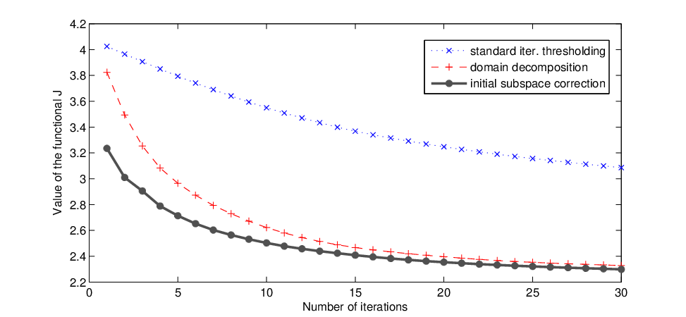
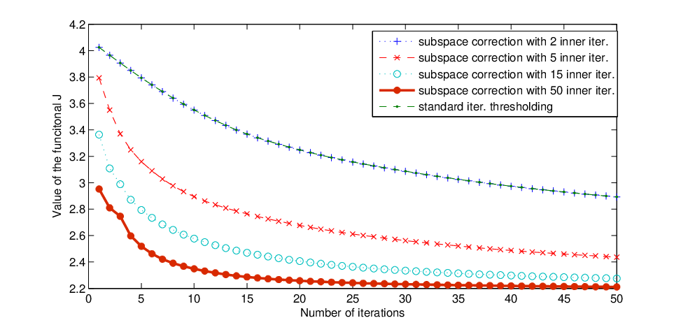
Refer to caption

Fig. 9: We show the application of the algorithms (1), (3), and (15) where the first 4 external iterations are performed with Q=VQ=V, followed by iterations where Q=IQ=I. Again the minimization of 𝒥\mathcal{J} is performed assuming that TT is a random matrix 200×40200\times 40 with Gaussian entries and the same parameters as in the previous figures. The starting acceleration due to the initial choice of Q=VQ=V allows to recover sufficient information on the support of the sparse minimal solution, so that the following iterations for Q=IQ=I do already perform significantly better than (3).

Refer to caption

Fig. 10: We show the application of the algorithms (1) and (15) (with the switching from Q=VQ=V to Q=IQ=I as in the previous figure) for the minimization of 𝒥\mathcal{J} where TT is a random matrix 200×40200\times 40 with Gaussian entries. We considered in this application of (15) 𝒩=10\mathcal{N}=10 subspaces ViV_{i}, α=0.005\alpha=0.005, 5050 external iterations and an increasing number of inner iterations for the minimization on each ViV_{i}, i=1,…,5i=1,\dots,5. We fixed a maximal number of 2020 iterations in the approximate computation of the auxiliary η\eta’s in (13). We can observe that by increasing the number of inner iterations we can significantly improve the rate of convergence with respect to the external iterations.

We developed further experiments for the evaluation of the behavior of the algorithm (15) with respect to other parameters, in particular the number of inner iterations for the minimization on each ViV_{i}, i=1,…,𝒩i=1,\dots,\mathcal{N}, and the number 𝒩\mathcal{N} of subspaces. In Figure 10 we show that by increasing the number of inner iterations we improve significantly the convergence with respect to the outer iterations. Of course, the improvement due to an increased number of inner iterations corresponds also to an increased computational effort. In order to counter-balance this additional cost one may consider a larger number of subspaces, that in turns implies a smaller dimension of each subspace. Indeed, note that inner iterations on subspaces with smaller dimension require a much less number of algebraic operations. In Figure 11 we show that by increasing the number of subspaces and, correspondingly, the number of inner iterations we do keep improving the convergence significantly. Hence, the parallel algorithm (31) adapted to a large number of subspaces performs very fast as soon as the inner iterations are also increased correspondingly.
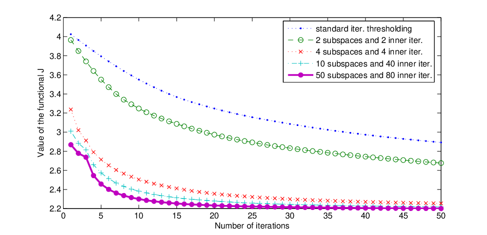
Refer to caption

Fig. 11: We show the application of the algorithms (1) and (15) (with the switching from Q=VQ=V to Q=IQ=I after 44 external iterations) for the minimization of 𝒥\mathcal{J} where TT is a random matrix 200×40200\times 40 with Gaussian entries. We considered in this application of (15) an increasing number 𝒩=2,4,10,50\mathcal{N}=2,4,10,50 of subspaces ViV_{i} and correspondingly an increasing number, 2,4,40,802,4,40,80, of inner iterations. Again we fixed α=0.005\alpha=0.005, 5050 external iterations, and a maximal number of 2020 iterations in the approximate computation of the auxiliary η\eta’s in (13). We can observe that by increasing the number of subspaces and inner iterations we can significantly improve the rate of convergence with respect to the external iterations.

8 Conclusion

Optimization of functionals promoting sparse recovery, e.g., ℓ1\ell_{1}-minimization and total variation minimization (where the sparsity is at the level of derivatives), were proposed in order to extract few significant features of the solution originally defined in very high dimensions. As a matter of fact, these minimizations cannot be performed by ordinary methods when the dimension scale is extremely large, for speed, resources, and memory restrictions. Hence, domain decomposition or subspace correction methods have to be invoked in these cases. Our work contributes to remedy the lack of such methods for these specific problems. We introduced parallel and alternating optimization algorithms on sequences of orthogonal subspaces of a Hilbert space, for the minimization of energy functionals involving convex constraints coinciding with semi-norms for a subspace. We provided an efficient numerical method for the implementation of the algorithm via oblique thresholding, defined by suitable Lagrange multipliers. It is important to notice that, on the one hand, these algorithms are realized by re-utilizing the basic building blocks of standard proximity-map iterations, e.g., projections onto convex sets, no significant complications in the implementations occur. On the other hand, several tricks can be applied in order to limit the computational load produced by the multiple iterations occurring on several subspaces (compare subsection 7.1.4). We investigated the convergence properties of the algorithms, providing sufficient conditions for ensuring the convergence to minimizers. We showed the applicability of these algorithms in delicate situations, like in domain decomposition methods for singular elliptic PDE’s with discontinuous solutions in 1D and 2D, and in accelerations of ℓ1\ell_{1}-minimizations. The numerical experiments nicely confirm the results predicted by the theory.

Acknowledgments

The authors thank Peter A. Markowich and the Applied Partial Differential Equations Research Group of the Department of Applied Mathematics and Theoretical Physics, Cambridge University, for the hospitality and the fruitful discussions during the late preparation of this work. M. Fornasier thanks Ingrid Daubechies for the intensive discussions on sparse recovery and the Program in Applied and Computational Mathematics, Princeton University, for the hospitality, during the early preparation of this work. M. Fornasier acknowledges the financial support provided by the European Union’s Human Potential Programme under contract MOIF-CT-2006-039438. C.-B. Schönlieb acknowledges the financial support provided by the Wissenschaftskolleg (Graduiertenkolleg, Ph.D. program) of the Faculty for Mathematics at the University of Vienna, supported by the Austrian Science Fund. The results of the paper also contribute to the project WWTF Five senses-Call 2006, Mathematical Methods for Image Analysis and Processing in the Visual Arts.

References

  • [1] L. Ambrosio, N. Fusco, and D. Pallara, Functions of bounded variation and free discontinuity problems., Oxford Mathematical Monographs. Oxford: Clarendon Press. xviii, 2000.
  • [2] G. Aubert and P. Kornprobst, Mathematical Problems in Image Processing. Partial Differential Equations and the Calculus of Variation, Springer, 2002.
  • [3] G. Aubert and L. Vese, A variational method in image recovery., SIAM J. Numer. Anal. 34 (1997), no. 5, 1948–1979.
  • [4] R. Baraniuk, Compressive sensing, Lecture Notes in IEEE Signal Processing Magazine, Vol. 24, July 2007.
  • [5] V. Barbu and T. Precupanu, Convexity and Optimization in Banach Spaces, 1996.
  • [6] H. H. Bauschke, F. Deutsch, H. Hundal, and S-H. Park, Accelerating the convergence of the method of alternating projections, Trans. Americ. Math. Soc. 355 (2003), no. 9, 3433–3461.
  • [7] J. H. Bramble, J. E. Pasciak, J. Wang, and J. Xu, Convergence estimates for product iterative methods with applications to domain decomposition, Math. Comp. 57 (1991), no. 195, 1–21.
  • [8] H. H. Bauschke, J. M Borwein, and A. S. Lewis, The method of cyclic projections for closed convex sets in Hilbert space. Recent developments in optimization theory and nonlinear analysis, (Jerusalem, 1995), 1–38, Contemp. Math., 204, Amer. Math. Soc., Providence, RI, 1997
  • [9] R. E. Bruck and S. Reich, Nonexpansive projections and resolvents of accretive operators in Banach spaces. Houston J. Math. 3 (1977), no. 4, 459–470
  • [10] E. J. Candès, Compressive sampling, Int. Congress of Mathematics, 3, pp. 1433-1452, Madrid, Spain, 2006
  • [11] E. J. Candès, J. Romberg, and T. Tao, Exact signal reconstruction from highly incomplete frequency information, IEEE Trans. Inf. Theory 52 (2006), no. 2, 489–509.
  • [12] E. J. Candès and T. Tao, Near Optimal Signal Recovery From Random Projections: Universal Encoding Strategies?, IEEE Trans. Inf. Theory 52 (2006), no. 12, 5406–5425.
  • [13] A. Chambolle, An algorithm for total variation minimization and applications. J. Math. Imaging Vision 20 (2004), no. 1-2, 89–97.
  • [14] A. Chambolle and P.-L. Lions, Image recovery via total variation minimization and related problems., Numer. Math. 76 (1997), no. 2, 167–188.
  • [15] T. F. Chan and T. P. Mathew, Domain decomposition algorithms, Acta Numerica (1994), 61–143.
  • [16] S. S. Chen, D. L. Donoho, M. A. Saunders, Atomic decomposition by basis pursuit. Reprinted from SIAM J. Sci. Comput. 20 (1998), no. 1, 33–61.
  • [17] J. F. Claerbout and F. Muir, Robust modeling with erratic data, Geophysics, vol. 38, no. 5, pp. 826–844, Oct. 1973.
  • [18] P. L. Combettes and V. R. Wajs, Signal recovery by proximal forward-backward splitting, Multiscale Model. Simul., 4 (2005), no. 4, 1168–1200.
  • [19] I. Daubechies, M. Defrise, and C. DeMol, An iterative thresholding algorithm for linear inverse problems, Comm. Pure Appl. Math. 57 (2004), no. 11, 1413–1457.
  • [20] I. Daubechies, M. Fornasier, and I. Loris, Acceleration of the projected gradient method for linear inverse problems with sparsity constraints, to appear in J. Fourier Anal. Appl., (2007).
  • [21] I. Daubechies, G. Teschke, and L. Vese, Iteratively solving linear inverse problems under general convex constraints, Inverse Probl. Imaging 1 (2007), no. 1, 29–46.
  • [22] D. C. Dobson and C. R. Vogel, Convergence of an iterative method for total variation denoising, SIAM J. Numer. Anal. 34 (1997), no. 5, 1779–1791.
  • [23] D. L. Donoho, Compressed sensing, IEEE Trans. Inf. Theory 52 (2006), no. 4, 1289–1306.
  • [24] D. L. Donoho and B. F. Logan, Signal recovery and the large sieve, SIAM J. Appl. Math. 52 (1992), no. 2, 577–591.
  • [25] D. L. Donoho and P. B. Stark, Uncertainty principles and signal recovery, SIAM J. Appl. Math. 49 (1989), no. 3, 906–931.
  • [26] I. Ekeland and R. Temam, Convex analysis and variational problems. Translated by Minerva Translations, Ltd., London., Studies in Mathematics and its Applications. Vol. 1. Amsterdam - Oxford: North-Holland Publishing Company; New York: American Elsevier Publishing Company, Inc., 1976.
  • [27] H.W. Engl, M. Hanke, and A. Neubauer, Regularization of inverse problems., Mathematics and its Applications (Dordrecht). 375. Dordrecht: Kluwer Academic Publishers., 1996.
  • [28] L. C. Evans and R. F. Gariepy, Measure Theory and Fine Properties of Functions., CRC Press, 1992.
  • [29] M. Fornasier, Domain decomposition methods for linear inverse problems with sparsity constraints, Inverse Problems 23 (2007), 2505–2526.
  • [30] M. Fornasier and H. Rauhut, Recovery algorithms for vector valued data with joint sparsity constraints, SIAM J. Numer. Anal. (2007), to appear.
  • [31] M. Fornasier and H. Rauhut, Iterative thresholding algorithms, Appl. Comput. Harmonic Anal. (2007), doi:10.1016/j.acha.2007.10.005, to appear.
  • [32] Y-J. Lee, J. Xu, and L. Zikatanov, Successive subspace correction method for singular system of equations, Fourteenth International Conference on Domain Decomposition Methods (I. Herrera, D. E. Keyes, O. B. Widlund, and R. Yates, eds.), UNAM, 2003, pp. 315–321.
  • [33] P. L. Lions, On the Schwarz alternating method, Proc. First Internat. Sympos. on Domain Decomposition Methods for Partial Differential Equations (R. Glowinski, G. H. Golub, G. A. Meurant, and J. Périaux, eds.), SIAM, Philadelphia, PA, 1988.
  • [34] R. Nabben and D.B. Szyld, Schwarz iterations for symmetric positive semidefinite problems, Research Report 05-11-03, Department of Mathematics, Temple University, 2005.
  • [35] Z. Opial, Weak convergence of the sequence of successive approximations for nonexpansive mappings, Bull. Amer. Math. Soc. 73 (1967), 591–597.
  • [36] A. Quarteroni and A. Valli, Domain decomposition methods for partial differential equations, Numerical Mathematics and Scientific Computation, The Clarendon Press Oxford University Press, New York, 1999, Oxford Science Publications.
  • [37] R.T. Rockafellar and R.J.B. Wets, Variational analysis, Grundlehren der Mathematischen Wissenschaften, vol. 317, Springer-Verlag, Berlin, 1998.
  • [38] M. Rudelson, R. Vershynin, Sampling from large matrices: an approach through geometric functional analysis, Journal of the ACM, to appear.
  • [39] L. I. Rudin, S. Osher, and E. Fatemi, Nonlinear total variation based noise removal algorithms., Physica D 60 (1992), no. 1-4, 259–268.
  • [40] F. Santosa and W. W. Symes, Linear inversion of band-limited reflection seismograms, SIAM J. Sci. Stat. Comput., vol. 7, no. 4, pp. 1307–1330, 1986.
  • [41] J.-L. Starck, E. J. Candès, D. L. Donoho, The curvelet transform for image denoising, IEEE Trans. Image Process. 11 (2002), no. 6, 670–684.
  • [42] H. L. Taylor, S. C. Banks, and J. F. McCoy, Deconvolution with the ℓ1\ell_{1} norm, Geophysics, vol. 44, no. 1, pp. 39–52, Jan. 1979.
  • [43] R. Tibshirani, Regression shrinkage and selection via the lasso, J. Roy. Statist. Soc. Ser. B 58 (1996), no. 1, 267–288.
  • [44] J. A. Tropp, On the conditioning of random subdictionaries, to appear in Appl. Comput. Harmonic Anal., (2007).
  • [45] L. Vese, A study in the BV space of a denoising-deblurring variational problem., Appl. Math. Optim. 44 (2001), 131–161.
  • [46] C. R. Vogel and M. E. Oman, Iterative methods for total variation denoising, SIAM J. Sci. Comput. 17 (1996), no. 1, 227–238, Special issue on iterative methods in numerical linear algebra (Breckenridge, CO, 1994).
  • [47] J. Xu, Iterative methods by space decomposition and subspace correction, SIAM Rev. 34 (1992), no. 4, 581–613.
  • [48] J. Xu and L. Zikatanov, The method of alternating projections and the method of subspsce corrections in Hilbert space, Report AM223, Department of Mathematics, Pann State University, 2000.