Next-to-MLLA corrections to single inclusive ${k_{{}_{\perp}}}$-distributions and 2-particle correlations in a jetLaboratoire de Physique Théorique d’Annecy-le-Vieux, UMR 5108LPTHE, UMR 7589 du CNRS associée à l’Université P. et M. Curie - Paris 6

As a consequence of the probabilistic shower picture, the notion of Generating Functional (GF) was proved suitable to understand and include higher order corrections to DLA asymptotics (see Basics and references therein).

The single inclusive spectrum and the $n$-particle momentum correlations can be derived from the MLLA Master Equation for the GF $Z=Z(u)$ Basics after successively differentiating with respect to a certain probing function $u=u(k)$; $k$ denotes the quadri-momentum of one parton inside the shower and the solution of the equations are written as a perturbative expansion in $\alpha_{s}$. At high energies this expansion can be resummed and the leading contribution be represented as an exponential of the anomalous dimension $\gamma(\alpha_{s})$; since further details to this logic can be found in Basics; RPR2, we only give the symbolic structure of the equation for the GF and its solution as

where $\gamma(\alpha_{s})$ can be written as an expansion in powers of $\sqrt{\alpha}_{s}$

The equation in (1) applies to each vertex of the cascade and its solution represents the fact that successive and independent partonic splittings inside the shower, such as the one displayed in Fig. 1, exponentiate with respect to the evolution-time parameter $dy=d\Theta/\Theta$; $\Theta\ll 1$ is the angle between outgoing couples of partons. The choice of $y$ follows from Angular Ordering (AO) in intrajet cascades; it is indeed the suited variable for describing time-like evolution in jets. Thus, Eq. (1) incorporates the Markov chains of sequential angular ordered partonic decays which are singular in $\Theta$ and $\gamma(\alpha_{s})$ determines the rate of inclusive quantities growth with energy.

While DLA treats the emission of both particles as independent by keeping track of the first term $\sim\sqrt{\alpha}_{s}$ in (2) without constraint, the exact solution of the MLLA evolution equation (partially) fulfills the energy conservation in each individual splitting process ($z+(1-z)=1$) by incorporating higher order ($\alpha_{s}^{n/2},n>1$) terms to the anomalous dimension. Symbolically; the first two analytical steps towards a better account of these corrections in the MLLA, NMLLA evolution, which we further discuss in II.3, can be represented in the form

where $\ell=\ln(1/x)\sim\alpha_{s}^{-1/2}$ with $x\ll 1$ (fraction of the jet energy taken away by one hadron), $z\sim 1$ for hard partons splittings such as $g\to q\bar{q}$…(this is in fact the region where the two partons are strongly correlated).

Energy conservation is particularly important for energetic particles as the remaining phase space is then very limited. On the other hand, a soft particle can be emitted with little impact on energy conservation. Some consequences of this behavior have also been noted in KLO:

• $(i)$

  the soft particles follow the features expected from DLA;

• $(ii)$

  there is no energy dependence of the soft spectrum;

• $(iii)$

  the ratio of soft particles $r=N_{g}/N_{q}$ in gluon and quark jets is consistent with the DLA prediction $N_{c}/C_{F}=9/4$ (see the measurement by DELPHI lepdelphi).

This is quite different from the ratio of global multiplicities which acquires large corrections beyond DLA (see, for example Fig.18 in the second reference given in Dremin2). For this quantity the HERWIG parton shower model corresponding to MLLA and exact energy conservation (same Fig. 18) and the full summation of the perturbative series of MLLA evolution equation (see also LO) come close to the data at $r=N_{g}/N_{q}\approx 1.5$ at LEP energies. As an intermediate example, we can mention the successful description of the semi-soft particle $\ln(1/x)$ distribution (“hump-backed plateau”) where the first correction (MLLA), despite the large value of the expansion parameter $\sqrt{\alpha}_{s}\approx 0.35$, already gives a good description of the data at the $Z^{0}$ peak ($Q=91.2$ GeV) of the $e^{+}e^{-}$ annihilation into a $q\bar{q}$ pair OPALZ0.

We study the formation of hadrons inside a jet produced in high-energy scattering processes, such as $e^{+}e^{-}$ annihilation or $pp$ and $p\bar{p}$ collisions. A jet of total opening angle $\Theta_{0}$ is initiated by a parton A (either a quark, $Q$, or a gluon, $G$) with energy $E$; A then splits into partons B and C, with energy fractions $z$ and $(1-z)$ respectively, forming a relative angle $\Theta$ (see Fig. 1). At the end of the cascading process, the parton B fragments into a hadron $h$ with energy $xE$, with the fragmentation function

which describes the distribution of the hadron $h$ inside the sub-jet B with an energy-fraction $x/z$.

As a consequence of AO in parton cascades, the functions $Q(z)$ and $G(z)$ satisfy the system of two-coupled integro-differential evolution equations RPR2:

with $\alpha_{s}$, the running coupling constant of QCD, given by

and where we define

following the notations of Ref. Basics; the MLLA equations above follow from the GF logic commented in the introductory paragraph. The scale $Q_{0}$ appearing in (7) is the collinear cut-off parameter, $\Lambda_{{}_{{}_{\rm QCD}}}$ is the non-perturbative scale of QCD which we set to 250 MeV in this work ¹¹ 1 NMLLA corrections arising from varying $\Lambda_{{}_{{}_{\rm QCD}}}$ are studied in detail in subsection III.5. , and

is the first term in the perturbative expansion of the $\beta$-function ($N_{c}$ is the number of colors, $T_{R}=n_{f}/2$ where $n_{f}=3$ is the number of light quark flavors). We only consider in this work the 1-loop expression for the running coupling constant, assuming that the role of the conservation of energy is much more important than the effects of 2-loop corrections to $\alpha_{s}$, as seen for instance in the case of multiplicity distributions Dremin2; we shall discuss this further in Section VI.1. The coupling constant $\alpha_{s}$ is also linked to the DLA anomalous dimension $\gamma_{0}$ of twist-2 operators by

In Eqs. (4) and (5), $\Phi_{\tt A}^{\tt B}(z)$ represent the one-loop DGLAP splitting functions Basics and we note:

In the small $x\ll z$ limit which we consider here, the fragmentation functions behave as

where $\rho_{\tt B}^{h}$ is a slowly varying function of the two logarithmic variables $\ln(z/x)$ and $y$ HBP that describes the hump-backed plateau.

The resummation scheme at MLLA is discussed in RPR2, in which $G(z)$ and $G(1-z)$ were replaced by $G(1)$ in the non-singular part of the integrands in Eqs. (4) and (5). In the present work, we calculate next-to-MLLA (NMLLA) corrections from the Taylor expansion of $\rho_{\tt B}^{h}$ in the variables $\ln z$ and $\ln(1-z)$ in the domain:

corresponding to hard parton splittings. To first order,

or, equivalently, for the function $B(z)$:

The derivative with respect to $\ln z$ or $\ln(1-z)$ has been replaced by the one with respect to $\ell$ because of (10) and the property that, at low $x$, $B$ is a function of $(\ln z+\ell)$ or $(\ln(1-z)+\ell)$. Since $\ell={{\cal{O}}}\left(1/\sqrt{\alpha_{s}}\right)$ (see Basics) the above expansion can be written symbolically

The terms proportional to $B_{\ell}$ thus provide NMLLA corrections to the solutions of the MLLA evolution equations (4) and (5).

The double differential distribution ${\rm d}^{2}N/({\rm d}x\,{\rm d}\ln\theta)$ for the production of a single hadron $h$ at angle $\Theta$ in a high energy jet of total energy $E$ and opening angle $\Theta_{0}\geq\Theta$, carrying the energy fraction $x$, is obtained by integrating the inclusive double differential 2-particle cross section (see PerezMachet) ⁵⁵ 5 The basic process under consideration is accordingly the emission of two hadrons, $h_{1}$ and $h_{2}$, inside a jet produced in a high-energy collision. Since the notations and kinematics are identical to the ones used in PerezMachet, the reader is referred to this work for a more detailed description.. Then, the single-inclusive $k_{\perp}$-distribution of hadrons inside a jet is obtained by integrating ${\rm d}^{2}N/({\rm d}{x}\,{\rm d}\!\ln\theta)$ over all energy-fractions $x$:

As in PerezMachet, a lower bound of integration, $\ell_{\rm min}$, is introduced since the present calculation is only valid in the small-$x$ region, and therefore cannot be trusted when $\ell\equiv\ln(1/x)$ becomes “too” small. We shall discuss this in more detail in Section III.3 and Appendix G.

According to PerezMachet, $\frac{{\rm d}^{2}N}{{\rm d}x\,{\rm d}\ln{\Theta}}$ can be expressed as

where $F_{{\tt A_{0}}}^{h}$, which represents the inclusive production of $h$ in the sub-jet of opening angle $\Theta$ inside the jet $A_{0}$ of opening angle $\Theta_{0}$, is given by a convolution product of two fragmentation functions PerezMachet:

The convolution expresses the correlation between the energy flux of the jet and one particle within it. Eq. (30) is schematically depicted in Fig. 2: $u$ is the energy-fraction of the intermediate parton ${\tt A}$, $D_{{\tt A_{0}}}^{\tt A}$ describes the probability to emit A with energy $uE$ off the parton $\tt{{\tt A_{0}}}$ (which initiates the jet) taking into account the evolution of the jet between $\Theta_{0}$ and $\Theta$, and $D_{\tt A}^{h}$ describes the probability to produce the hadron $h$ off A with energy fraction $x/u$ and transverse momentum $k_{\perp}\approx uE\Theta\geq Q_{0}$; $k_{\perp}$ is defined with respect to the jet axis which is, in this context, identified with the direction of the energy flux.

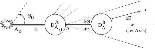
As discussed in PerezMachet, the convolution (30) is dominated by $u={{\cal{O}}}\left(1\right)$. Therefore, $D_{{\tt A_{0}}}^{\tt A}\left(u,E\Theta_{0},uE\Theta\right)$ is given by DGLAP evolution equations. On the contrary, since $x\ll{u}={{\cal{O}}}\left(1\right)$ in the small-$x$ limit where MLLA evolution equations are valid, $D_{\tt A}^{h}$ behaves as (see (10))

Since $Y_{\Theta}+\ln u=\ell+\ln u+y$, the hump-backed plateau $\rho_{\tt A}^{h}$ depends on the two variables $\ell+\ln u$ and $y$, and we conveniently define $\tilde{D}$ as:

The Taylor expansion of $\rho_{\tt A}^{h}$ to the second order in $\ln u$ for $u\sim 1\Leftrightarrow|\ln u|\ll 1$, that is, one step further than in PerezMachet, leads to

where

is the MLLA distribution calculated in PerezMachet. In (34) we have introduced first logarithmic derivatives of $\tilde{D}_{\tt A}^{h}$

Thus, as in PerezMachet, in the soft limit the correlation disappears and the convolution (30) is reduced to the factorized expression in (33).

The second term in the r.h.s. of (33) is the new NMLLA correction calculated in this paper. Since $x/u$ is small, the inclusive spectrum $\tilde{D}_{\tt A}^{h}(\ell,y)$ occurring in (33) should be taken as the next-to-MLLA solution of the evolution equations (23) and (24). However, as already mentioned and shown in Appendix B, the MLLA inclusive spectrum for a gluon jet can be used as a good approximation for (24) (with $a_{1}\neq 0,a_{2}=0$) such that, in (34), it is enough to use this level of approximation. So, we shall therefore use Eqs. (26) and (II.4.3) in the following.

The NMLLA correction in (33) globally decreases $|xF_{{\tt A_{0}}}^{h}|$ in the perturbative region ($y\geq 1.5$). Indeed, while the MLLA part proportional to $\ln u$ in (34) is negative PerezMachet, it is instead, there, positive because of the positivity of $u$ and $\ln^{2}u$ and $\frac{{\rm d}^{2}\tilde{D}_{\tt A}^{h}}{{\rm d}\ell^{2}}\simeq\frac{{\rm d}^{2}G}{{\rm d}\ell^{2}}$ (see Fig. 18 in Appendix C). The NMLLA contribution therefore tempers somehow the size of the MLLA corrections when $y$ is large enough.

The function $F_{{\tt A_{0}}}^{h}$ is related to the inclusive gluon distribution via the color currents defined as Basics; PerezMachet

The color current can be seen as the average color charge carried by the parton A due to the DGLAP evolution from ${\tt A_{0}}$ to A. Introducing the first and second logarithmic derivatives of $\tilde{D}_{\tt A}^{h}$,

which are MLLA and NMLLA corrections, respectively, Eq. (33) can now be written

where

Unlike in PerezMachet at MLLA, using the approximation $u={{\cal{O}}}\left(1\right)$ to replace in (38) $uE\Theta$ by $E\Theta$ requires here some care, since the resulting scaling violation of the DGLAP fragmentation functions also provides ${\cal O}(\alpha_{s})$ corrections to $\langle u\rangle$. Explicit calculations (see Appendix D) show that they never exceed $5\%$ of the leading term. Accordingly, we neglect them in the following and replace (38) by

The total average color current $\langle C\rangle_{{\tt A_{0}}}$ of partons caught by the calorimeter decomposes accordingly into three terms which can be written:

The leading order (LO) ${{\cal{O}}}\left(1\right)$ and MLLA ${{\cal{O}}}\left(\sqrt{\alpha_{s}}\right)$ contributions to the color currents have been determined in PerezMachet. The new NMLLA ${{\cal{O}}}\left(\alpha_{s}\right)$ correction evaluated in this paper reads

assuming $Q=C_{F}/N_{c}\ G$. We checked that using instead the NMLLA exact formula (27) for the quark inclusive spectrum $Q$ actually leads to negligible corrections to the color currents (see Appendix E). Eq. (41) can be obtained from the Mellin-transformed DGLAP fragmentation functions

through the formula

Given the rather lengthy expressions, the complete analytic results for $\langle C\rangle^{\rm NMLLA-MLLA}_{{\tt A_{0}}}$ for quark and gluon jets are given in Appendix F.

For illustrative purposes, the color currents are plotted in Fig. 3 in the limiting spectrum approximation ($\lambda=0$). The LO (solid line), MLLA (dash-dotted) and NMLLA (dashed) currents are computed for a quark (left) and for a gluon jet (right) with energy $Y_{\Theta_{0}}=6.4$ – corresponding to Tevatron energies – and at fixed $\ell=2$. As can be seen in Fig. 3, NMLLA ${{\cal{O}}}\left(\alpha_{s}\right)$ corrections to the MLLA color currents are clearly not negligible, yet of course somewhat smaller than the MLLA ${{\cal{O}}}\left(\sqrt{\alpha_{s}}\right)$ corrections to the LO result. In the perturbative region ($y>1.5$), these corrections are positive and consequently decrease the difference with the LO estimate. On the contrary, at small $y\leq 1.5$, the corrections are rather large and negative coming from the negative sign of $G_{\ell\ell}(\ell,y)$ (see Fig. 18 in Appendix C). However, it should be kept in mind that as $y$ goes to $0$, ${k_{{}_{\perp}}}$ gets closer to $\Lambda_{{}_{{}_{\rm QCD}}}$ (remind that $Q_{0}=\Lambda_{{}_{{}_{\rm QCD}}}$ in the limiting spectrum approximation) and, thus, the present perturbative predictions may not be reliable in this domain.

Note also that both the MLLA and NMLLA corrections vanish at $y=0$ (since $G_{\ell}=G_{\ell\ell}=0$) and when $\Theta=\Theta_{0}$. Another interesting property to mention is the decrease of MLLA and NMLLA corrections as $\ell$ increases, that is, when partons get softer and recoil effects more negligible.

References

- (1)
Yu.L. Dokshitzer, V.S. Fadin, V.A. Khoze, Coherent effects in the
perturbative QCD parton jets, Phys. Lett. B 115 (1982) 242;
Ya.I. Azimov, Yu.L. Dokshitzer, V.A. Khoze, S.I. Troian, Humpbacked QCD Plateau in Hadron Spectra, Z. Phys. C 31 (1986) 213;
C.P. Fong, B.R. Webber, Higher order QCD corrections to hadron energy distribution in jets, Phys. Lett. B 229 (1989) 289. - (2) V.A. Khoze, W. Ochs, Perturbative QCD approach to multiparticle production, Int. J. Mod. Phys. A 12 (1997) 2949.
- (3)
Ya.I. Azimov, Yu.L. Dokshitzer, V.A. Khoze, S.I. Troian,
Similarity of Parton and Hadron Spectra in QCD Jets,
Z. Phys C 27 (1985) 65;
Yu.L. Dokshitzer, V.A. Khoze, S.I. Troian, On the concept of local parton hadron duality, J. Phys. G 17 (1991) 1585. - (4) R. Pérez Ramos, B. Machet, MLLA inclusive hadronic distributions inside one jet at high energy colliders, [hep-ph/0512236], JHEP 04 (2006) 043.
- (5) R. Pérez Ramos, Two particle correlations inside one jet at Modified Leading Logarithmic Approximation of Quantum Chromodynamics; I: Exact solution of the evolution equations at small , [hep-ph/0605083], JHEP 06 (2006) 019 and references therein.
- (6) R. Pérez Ramos, Single inclusive distribution and two-particle correlations inside one jet at modified leading logarithmic approximation of quantum chromodynamics: II. Steepest descent evaluation at small , [hep-ph/0607223], JHEP 09 (2006) 014.
- (7) CDF collaboration, S. Jindariani, A. Korytov, A. Pronko, Distributions of Particles in Jets at CDF, CDF report CDF/ANAL/JET/PUBLIC/8406 (March 2007), www-cdf.fnal.gov/physics/new/qcd/ktdistributions_06/cdf8406_Kt _jets_public.ps.
- (8) Yu.L. Dokshitzer, V.A. Khoze, A.H. Mueller, S.I. Troyan, Basics of Perturbative QCD, (Editions Frontières, Gif-sur-Yvette, 1991).
- (9) F. Cuypers, K. Tesima, Recoil effect on multiplicity correlation, Z. Phys. C 54 (1992) 87.
- (10) Yu.L. Dokshitzer, Improved QCD treatment of the KNO phenomenon, Phys. Lett. B 305 (1993) 295.
- (11) F. Arleo, R. Pérez-Ramos, B. Machet: “Hadronic single inclusive distributions inside one jet beyond MLLA”, arXiv:07072391 [hep-ph], Phys. Rev. Lett. 100 (2008) 052002
- (12) V.A. Khoze, S. Lupia, W. Ochs, Perturbative description of particle spectra at LEP-1.5, Phys. Lett. B 386 (1996) 451.
- (13) DELPHI Collaboration: J. Abdallah et al., Coherent soft particle production in decay into three jets, [hep-ex/0410075], Phys. Lett. B 605 (2005) 37.
- (14)
I.M. Dremin, Quantum chromodynamics and multiplicity distributions,
[hep-ph/9406231], Phys. Usp. 37 (1994) 715;
ibid., Usp. Fiz. Nauk 164 (1994) 785;
I.M. Dremin, J.W. Gary, Hadron multiplicities, Phys. Rep. 349 (2001) 301. - (15) S. Lupia, W. Ochs, Unified QCD description of hadron and jet multiplicities, [hep-ph/9707393], Phys. Lett. B 418 (1998) 214.
- (16) OPAL Collaboration, M.Z. Akrawy et al., A study of coherence of soft gluons in hadron jets, Phys. Lett. B 247 (1990) 617.
- (17)
F.E. Low, Bremsstrahlung of Very Low-Energy
Quanta in Elementary Particle Collisions, Phys. Rev. 110 (1958) 974;
T.H. Burnett and N.M. Kroll, Extension of the Low soft photon theorem, Phys. Rev. Lett. 20 (1968) 86. - (18) I.M. Dremin, V.A. Nechitailo, Average multiplicities in gluon and quark jets in higher order perturbative QCD, [hep-ex/9406002], Mod. Phys. Lett. A9 (1994) 1471.
- (19) Yu.L. Dokshitzer, V.S. Fadin, V.A. Khoze, On the sensitivity of the inclusive distributions in parton jets to the coherence effects of QCD gluon cascades, Z. Phys C 18 (1983) 37.
- (20)
Yu.L. Dokshitzer, V.A. Khoze, S.I. Troian, Phenomenology of the
particle spectra in QCD jets in a modified leading logarithmic
approximation, Z. Phys. C 55 (1992) 107;
Yu.L. Dokshitzer, V.A. Khoze, S.I. Troian, Inclusive particle spectra from QCD cascades, Int. J. Mod. Phys. A 7 (1992) 1875;
V.A. Khoze, W. Ochs, J. Wosieck, Analytical QCD and multiparticle production, [hep-ph/0009298], and references therein. - (21) ALICE collaboration, ALICE physics performance report, volume II, B. Alessandro et al., J. Phys. G32 (2006) 1295.
- (22) CMS collaboration, CMS physics technical design report: Addendum on high density QCD with heavy ions, D. d’Enterria (Ed.) et al., J. Phys. G34 (2007) 2307.
- (23) K. Konishi, A. Ukawa and G. Veneziano, Jet Calculus: A Simple Algorithm for Resolving QCD Jets, Nucl.Phys. B 157 (1979) 45.
- (24)
C.P. Fong, B.R. Webber, One and two particle distributions
at small in QCD jets, Nucl. Phys. B 355 (1991) 54;
ibid., Two particle correlations at small in QCD jets, Phys. Lett. B 241 (1990) 255. - (25) I.M. Dremin, Cumulant and factorial moments in perturbative gluodynamics, Phys. Lett. B 313 (1993) 209.
- (26) I.M. Dremin, Jet calculus problems of the perturbative quantum chromodynamics, [hep-ph/0309193], Acta Phys. Polon. B 35 (2004) 417.
- (27) OPAL collaboration, P. D. Acton et al., A Study of two particle momentum correlations in hadronic decays, Phys. Lett. B 287 (1992) 401.
- (28) CDF collaboration, T. Aaltonen et al., Two-particle momentum correlations in jets produced in collisions at TeV, arXiv:0802.3182 [hep-ex].
- (29) S. Albino, B.A. Kniehl, G. Kramer, W. Ochs, Resummation of Soft Gluon Logarithms in the DGLAP Evolution of Fragmentation Functions, [hep-ph/0510319], Phys. Rev. D 73 (2006) 054020.
- (30) Yu.L. Dokshitzer, G. Marchesini, G.P. Salam, Revisiting parton evolution and the large- limit, [hep-ph/0511302], Phys. Lett. B 634 (2006) 504.
- (31) R.K. Ellis, W.J. Stirling, B.R. Webber, QCD and Collider Physics, Cambridge Monographs in Particle Physics, Nuclear Physics and Cosmology 8 (1996); see in particular Eqs. (4.122) and (6.22).