1150\Yearpublication2007 \Yearsubmission2007 \Month9\Volume328\Issue10\DOI10.1002/asna.200710859
2007 Dec 15
Stability of toroidal magnetic fields in the solar tachocline and beneath
Abstract
Stability of toroidal magnetic field in a stellar radiation zone is considered for the cases of uniform and differential rotation. In the rigidly rotating radiative core shortly below the tachocline, the critical magnetic field for instability is about 600 G. The unstable disturbances for slightly supercritical fields have short radial scales 1 Mm. Radial mixing produced by the instability is estimated to conclude that the internal field of the sun can exceed the critical value of 600 G only marginally. Otherwise, the mixing is too strong and not compatible with the observed lithium abundance. Analysis of joint instability of differential rotation and toroidal field leads to the conclusion that axisymmetric models of the laminar solar tachocline are stable to nonaxisymmetric disturbances. The question of whether sun-like stars can posses tachoclines is addressed with positive answer for stars with rotation periods shorter than about two months.
keywords
instabilities – magnetohydrodynamics (MHD) – stars: interiors – stars: magnetic fields – Sun: magnetic fields1 Introduction
The problem of stability of toroidal magnetic fields in stellar interiors first addressed by Tayler ([1973]) is highly relevant for the dynamics of stellar radiation zones. The stability controls which primordial fields can survive inside the stars on evolutionary time scales. Magnetic instabilities are important for transport of angular momentum and chemical species in the radiation zones (Barnes, Charbonneau & MacGregor [1999]). The stability problem is also relevant to the origin of the solar tachocline (Gilman [2005]).
This paper concerns the stability of toroidal magnetic fields in rotating radiation zones. The analysis is global in horizontal dimensions but the radial scales of unstable disturbances are assumed as short. The smallness of the radial scales is a consequence of the stable stratification. Our mathematical formulation is close to the thin layer approximation of Cally ([2003]) and Miesch & Gilman ([2004]). Our aims, however, are quite different. We do not address the growth rates of highly supercritical disturbances but focus on the marginal stability. We also include finite diffusion that is necessary when stability of rigidly rotating region beneath the tachocline is concerned. When diffusion is neglected, the most rapidly growing disturbances have indefinitely short radial scales and the instability can be excited by indefinitely small magnetic field. The unphysical zero wave lengths and field amplitudes are prevented by finite diffusion. The marginal field strength for the rigidly rotating region just beneath the tachocline is about 600 G. Estimation of the radial mixing produced by the instability suggests that the marginal value is close to the upper bound for the internal field. The mixing is too strong and is not compatible with the observed lithium abundance if the marginal value is considerably exceeded.
Differential rotation can drive its own instability even without magnetic fields (Watson [1981]; Dziembowski & Kosovichev [1987]). The instability has been extensively studied in 2D approximation of strictly horizontal disturbances. An account for radial displacements in our 3D formulation reduces the magnitude of differential rotation required for the hydrodynamic instability.
We find that axisymmetric models of a laminar solar tachocline do not suffer from nonaxisymmetric magnetic instabilities. The question arises whether stars other than the Sun can possess tachoclines. Evidences on stellar differential rotation used in combination with laminar tachocline theory provide a positive answer for all solar-like stars whose rotation is not too slow.
2 The model
The background state of our model includes differential rotation and toroidal magnetic field. The angular velocity distribution is parameterized as
| (1) |
where is the equatorial value of and is colatitude. The toroidal field is expressed in terms of the Alfvén angular frequency , i.e.
| (2) |
where is the azimuthal unit vector. The field is assumed to consist of two broad belts antisymmetric about the solar equator:
| (3) |
is the normalized field strength, means approximate equipartition of rotational and magnetic energies.
The equations for linear perturbations written in the Appendix were derived in Kitchatinov & Rüdiger ([2007]). The equations apply to the disturbances that are global in horizontal dimensions but short-scaled in radius. The reason why the radial scales are short is the stable (subadiabatic) stratification. The buoyancy frequency, ,
| (4) |
enters the normalized equations via the parameter
| (5) |
where is the gravity, is the heat capacity at constant pressure, is the specific entropy, is the (heliocentric) radius and is the radial wave number of the disturbances. The ratio in stellar radiation zones is a large quantity (Fig. 1). After Eq. (5), disturbances can avoid the stabilizing effect of stratification by decreasing their radial scales. Our results shall confirm this short-wave approximation with .

The equations for small disturbances listed in the Appendix allow two types of equatorial symmetry. We use the standard notations Sm and Am for symmetric and antisymmetric modes, is the azimuthal wave number. Sm modes have mirror-symmetry (about the equatorial plane) disturbances of the magnetic field (symmetric , and antisymmetric ), mirror-antisymmetric velocity (symmetric and antisymmetric and ) and antisymmetric perturbations of entropy . The symmetries reverse for Am modes. These symmetry conventions are the same as in Gilman, Dikpati & Miesch ([2007]).
3 Results and discussion
3.1 Beneath the tachocline ( = 0)
Helioseismology shows that the rotation below the tachocline is almost rigid (Schou et al. [1998]). The uniform rotation has minimum kinetic energy for given angular momentum. Rotational energy cannot, therefore, feed any instability so that magnetic instabilities can only be considered.
3.1.1 Ideal fluids
Microscopic diffusion in radiative cores is small and often neglected. We start with the case of ideal fluids with diffusion parameters equal zero. The stability map for this case is shown in Fig. 2.

Only the kink-type () disturbances are found unstable. The instability remains active for indefinitely small field amplitude though the range of radial scales of unstable excitations reduces with decreasing . Therefore, rotation does here not suppress the Tayler instability. The character of rotational influence crucially depends on the toroidal field profile. Pitts & Tayler ([1985]) found strong rotational suppression but suggested that it might be restricted to the case in which the ratio of rotational to Alfvén velocities is uniform. The results of Fig. 2 confirm the expectation. The results were found with same numerical code as formerly reported strong rotational quenching for uniform (Kitchatinov & Rüdiger [2007]).
The ideal instability for very weak fields is, however, of mainly academic interest because the unstable disturbances have indefinitely small radial scales. Finite diffusion must, therefore, be included.
3.1.2 Finite diffusion
From now on the finite values
| (6) |
that are characteristic of the upper part of the solar radiative core are used for the diffusion parameters (Eq. 14). The relation of Eq. (6) is typical of stellar radiation zones.
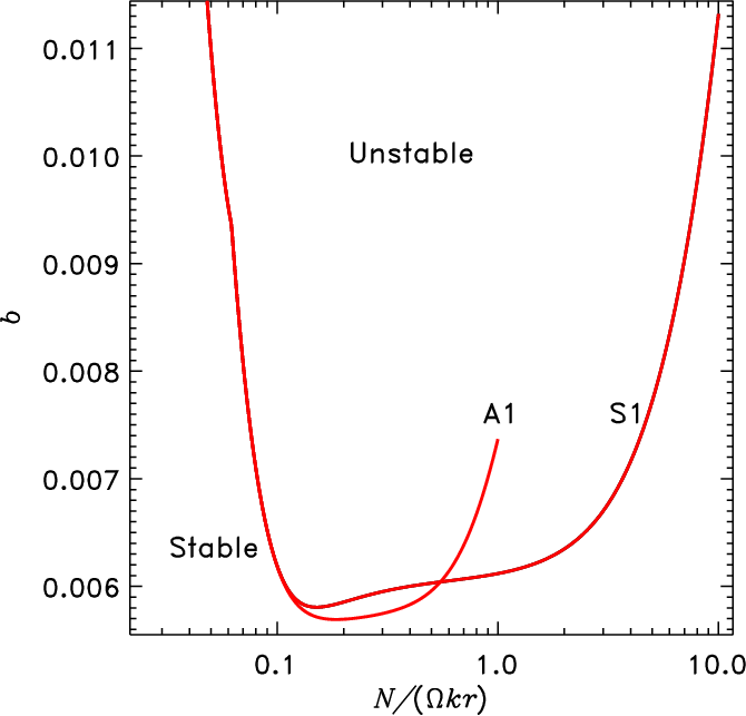
The stability map computed with finite diffusion is shown in Fig. 3. Small radial scales are now stable due to finite magnetic diffusivity.
For the upper radiation zone of the Sun with g/cm3 it follows
| (7) |
After Fig. 3, the critical magnetic field for the onset of the instability is thus about 600 G. The modes that first become unstable when this field strength is exceeded have vertical wavelengths between 1 and 2 Mm. For larger field strengths, there is a range of unstable wavelengths. The maximum growth rates remain, however, at the wavelengths Mm (Fig. 4). The growth rates are rather small.


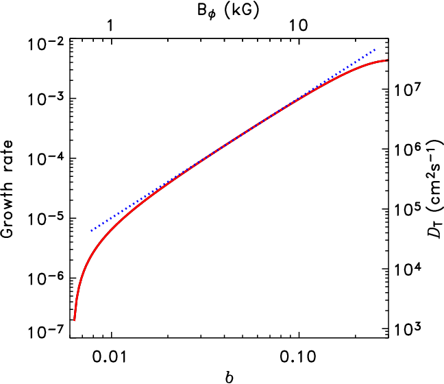
The instability radially mixes chemicals. It can thus be relevant for the radial transport of light elements (Barnes et al. [1999]). The effective diffusivity, can be estimated from our linear computations. With Eq. (7) this yields
| (8) |
where is the normalized growth rate given in Fig. 5. Diffusivities in excess of cm2s-1 in the upper radiative core are not compatible with the observed solar lithium abundance. Hence, the toroidal field amplitude can only slightly exceed the marginal value of about 600 G.
3.2 Inside the tachocline ( 0)
The helioseismology detections of the tachocline central radius and (equatorial) thickness (Charbonneau et al. [1999b]) place the tachocline mainly if not entirely beneath the base of convection zone at (Basu & Antia [1997]; Christensen-Dalsgaard, Gough & Thompson [1991]). The stability analysis of toroidal fields of radiative core can thus be applied to the tachocline. The differential rotation with in Eq. (1) must also be included.
3.2.1 Hydrodynamic stability
Differential rotation can be unstable even without magnetic fields. The hydrodynamic stability of the tachocline has been studied in 2D approximation of strictly horizontal displacements (Charbonneau, Dikpati & Gilman [1999a]; Garaud [2001]). Here we extend the treatment to 3D.

The resulting stability map is shown in Fig. 6. A1 and S2 modes can be unstable for positive . The marginal values of approach constants for large . The large- limit reproduces the results of the 2D theory as it should (Kitchatinov & Rüdiger [2007]). The minimum -value for the instability corresponds, however, to finite vertical scales of about 6 Mm.
3.2.2 Joint instabilities
Growth rates of joint instabilities for have been discussed by Cally ([2003]) and Gilman et al. ([2007]). Now we concern the marginal stability that is important in relation to the models of laminar tachocline formed by a weak internal magnetic field (Rüdiger & Kitchatinov [2007]).


Isolines of the very small growth rates for A1 and S1 modes for the and parameters of differential rotation and magnetic field are shown in Figs. 7 and 8. The growth rates are optimized in , i.e. has been varied to find the maximum growth rates for given and . From Sect. 3.2.1 we know that differential rotation is stable to S1 disturbances. For sufficiently large , the S1 modes become unstable for very small magnetic field (Fig. 8). The characteristic growth rates of this mode are nevertheless large compared to S2 disturbances.
The models for the laminar solar tachocline are valid for microscopic diffusivities or sufficiently low turbulent diffusivities up to about cm2/s (Kitchatinov & Rüdiger [2006]). According to Eq. (8), this means growth rates up to . The laminar tachocline models have toroidal field amplitudes of about 200 G or . The maximum field in the models is attained at those depths where latitudinal differential rotation is reduced to about 10%. Figures 7 and 8 show that the axisymmetric models for the laminar solar tachocline are stable to nonaxisymmetric disturbances.
3.2.3 Do stars other than the Sun possess tachoclines?
Observations of Barnes et al. ([2005]) and theoretical models of Kitchatinov & Rüdiger ([1999]) and Küker & Stix (2001) suggest that the absolute value of differential rotation is almost independent of the rotation rate for stars of given mass (but increases with mass). Figure 9 reformulates the stability map for the (most easily excited) A1 modes in terms of the magnetic field strength and angular velocity of a star of solar mass assuming and using Eqs. (2) and (3) to recover .

The toroidal field amplitude in the laminar tachocline models is controlled by and fluid density only. Therefore, the limit G of the solar tachocline model does also apply to the stars of same mass but different rotation rates. The star moves down on Fig. 9 along a vertical line of G as the star spins down with age. The toroidal field can be only mildly unstable () for the laminar tachocline model to apply. All solar mass stars with rotation periods shorter than about two months should thus possess tachoclines after Fig. 9.
Acknowledgements.
This work was supported by the Deutsche Forschungsgemeinschaft and by the Russian Foundation for Basic Research (project 05-02-16326).References
- [1999] Barnes, G., Charbonneau, P., MacGregor, K.B.: 1999, ApJ 511, 466
- [2005] Barnes, J.R., Cameron, A.C., Donati, J.-F., James, D.J., Marsden, S.C., Petit, P.: 2005, MNRAS 357, L1
- [1997] Basu, S., Antia, H.M.: 1997, MNRAS 287, 189
- [2003] Cally, P.S.: 2003, MNRAS 339, 957
- [1999a] Charbonneau, P., Dikpati, M., Gilman, P.A.: 1999a: ApJ 526, 523
- [1999b] Charbonneau, P., Christensen-Dalsgaard, J., Henning, R., Larsen, R.M., Schou, J., Thompson, M.J., Tomczyk, S.: 1999b, ApJ 527, 445
- [1991] Christensen-Dalsgaard, J., Gough, D.O., Thompson, M.J.: 1991, ApJ 378, 413
- [1987] Dziembowski, W., Kosovichev, A.G.: 1987, AcA 37, 341
- [2001] Garaud, P.: 2001, MNRAS 324, 68
- [2005] Gilman, P.A.: 2005, AN 326, 208
- [2007] Gilman, P.A., Dikpati, M., Miesch, M.S.: 2007, ApJS 170, 203
- [1999] Kitchatinov, L.L., Rüdiger, G.: 1999, A&A 344, 911
- [2006] Kitchatinov, L.L., Rüdiger, G.: 2006, A&A 453, 329
- [2007] Kitchatinov, L.L., Rüdiger, G.: 2007, astro-ph/0701847
- [2001] Küker, M., Stix, M.: 2001, A&A 366, 668
- [2004] Miesch, M.S., Gilman, P.A.: 2004, SoPh 220, 287
- [1985] Pitts, E., Tayler, R.J.: 1985, MNRAS 216, 139
- [1997] Rüdiger, G., Kitchatinov, L.L.: 1997, AN 318, 273
- [2007] Rüdiger, G., Kitchatinov, L.L.: 2007, NJPh 9, 302
- [1998] Schou, J., Antia, H.M., Basu, S., et al.: 1998, ApJ 505, 390
- [2002] Spruit, H. C.: 2002, A&A 381, 923
- [1990] Stix, M., Skaley, D.: 1990, A&A 232, 234
- [1973] Tayler, R.J.: 1973, MNRAS 161, 365
- [1981] Watson, M.: 1981, GApFD 16, 285
- [2007] Zahn, J.-P., Brun, A.S., Mathis, S.: 2007, A&A 474, 145
Appendix A Linear stability equations
The equations used in our stability analysis represent the eigenvalue problem resulting from the exponential time dependence of the disturbances. The dependencies on azimuth and radius are taken as Fourier modes . The equations are formulated in terms of scalar potentials for the vector magnetic and velocity fields (Kitchatinov & Rüdiger [2007]).
The equation for the potential of the poloidal flow reads
| (9) | |||||
where is the normalized radial wave length (5). The dimensionless eigenvalue , the angular velocity and the Alfvén angular frequency are all normalized to , , and
The complete system of five equations also includes the equation for the potential of toroidal flow
| (10) | |||||
the equation for the potential of toroidal magnetic disturbances
| (11) | |||||
the equation for the poloidal magnetic disturbances
| (12) |
and the equation for the entropy perturbations
| (13) |
The equations include finite diffusion via the parameters
| (14) |
where , , and are the viscosity, the magnetic diffusivity and the heat conductivity, respectively.
The disturbances in physical units can be recovered with
| (15) | |||||
and the vector magnetic and velocity fields can then be restored with
| (16) | |||||
where , and are unit vectors in radial, meridional and azimuthal directions, respectively.