Analytic models of ultra-cold atomic collisions at negative energies for application to confinement-induced resonances
Abstract
We construct simple analytic models of the -matrix, accounting for both scattering resonances and smooth background contributions for collisions that occur below the s-wave threshold. Such models are important for studying confinement-induced resonances such as those occurring in cold collisions of 133Cs atoms in separated sites of a polarization-gradient optical lattice. Because these resonances occur at negative energy with respect to the -wave threshold, they cannot be studied easily using direct numerical solutions of the Schrödinger equation. Using our analytic model, we extend previous studies of negative-energy scattering to the multichannel case, accounting for the interplay of Feshbach resonances, large background scattering lengths, and inelastic processes.
pacs
11.55.Bq,37.10.Jk,34.50.-s,02.30.Mv,I Introduction
The ability to control ultra-cold atom-atom interactions has opened the door to a wide variety of fundamental and applied studies, including the production of ultra-cold molecules jin1; ketterle1; grimm1; hulet1, simulations of condensed matter phenomena condmatsim; quantumhall, and quantum information processing uwe. The tools that have been central to this development include designer atom traps, for example, optical lattices opticallattice, and controllable scattering resonances such as a magnetic Feshbach resonance feshbach. Both of these can be used to manipulate the two-body scattering process, thus affecting the strength of the interaction, the nature of the resulting two-body states, and more general many-body phenomena. Examples include confinement-induced resonances cir, bound-states with repulsive interactions boundneg, and Feshbach resonances in band structures feshbachlattice.
A particular example that we have explored previously is a trap-induced resonance (TIR) that occurs as a result of interaction between atoms that are confined to spatially separated harmonic traps stockprl; tir. This happens as a consequence of a molecular bound state that becomes resonant with the vibrational state of the separated atoms due to a quadratic rise in the light shift when the two atoms approach one another, as shown schematically in Fig. 1. A strong resonance can occur when the confinement of the wave packet in the trap is on the order of (or smaller than) the free-space scattering length. This -wave resonance is analogous to a higher-partial wave shape resonance occurring in free space, but here the tunneling barrier arises from the trap rather than from an angular momentum centrifugal barrier. Because of this tunneling, the interaction occurs at “negative energy” values with respect to the free-particle -wave scattering threshold.

In previous work on the TIR in cesium tir, whose large scattering length gives rise to a strong resonance, Stock et al. extracted the scattering length at negative energy for the single channel case by an explicit integration of the radial Schrödinger equation at negative energies using the Numerov method. Such a procedure has limited utility; the solutions are unstable since the wave function blows up in the tunneling barrier. The situation gets very complicated as soon as there is more than one channel. A proper numerical technique must ensure that open channels are propagated along with the exponentially decaying closed channels while maintaining accuracy to relevant digits. Most coupled channel codes that incorporate such situations (i.e. propagating closed and open channels), eventually drop the closed channels beyond certain radius since they are only interested in open channels. On the other hand, the problem of TIR considered in this paper requires us to integrate to large enough radius for determining a good asymptotic log derivative (for both open and closed channels). We emphasize that we are not allowed to drop any channels, since in the end, we are required to extract the asymptotic log derivatives for both open as well as closed channels.
To remedy this, we consider here analytic models of the multichannel -matrix. Simplified analytic models have been employed in previous studies of ultra-cold collisions and scattering resonances. Julienne and Gao have predicted the properties of Feshbach resonances based on the analytic properties of the van der Waals long range potential julienneandgao. Marcelis et al. have used analytic models to describe the interplay of open and closed channels in the context of Feshbach resonances associated with a large background scattering length marcelis. These analytic models, while simple in nature, are able to encapsulate the necessary physics in just a few parameters. These parameters can then be incorporated into building model many-body Hamiltonians, an example being the two-channel model used for describing resonance superfluidity in a two component Fermi gas kokkelmansandholland.
Our goal in this article is to develop an analytic model that can be used to study the TIR for Cs atoms trapped in an optical lattice. In Sec. II we review the basic physics that gives rise to the TIR, its application in Cs, and show the limitations of direct numerical solutions, even for single channel scattering. Section III contains the heart of our new results. We review the basic resonant scattering phenomena and how they are modeled analytically in the -matrix. We then apply this to determine expressions for the negative-energy scattering length in a nontrivial multichannel scattering process, relevant to an experimental observation of the TIR. We summarize our results in Sec. IV.

II Scattering resonances in 133Cs
We consider the scattering of two 133Cs atoms in their 6S1/2 electronic ground state, trapped in an optical lattice. The Zeeman hyperfine structure of this manifold is shown in the Fig. 2 with magnetic sub-levels labeled as for convenience. Henceforth, all two-atom scattering channels will be denoted by the relevant pair of these sub-levels. To begin with, we consider the scattering in the channel. This is motivated by studies of controlled collisions via spin-dependent transport in polarization gradient lattices polgradcollisions. In these spin states, two atoms that are separated by in a lin-perp-lin optical lattice can be transported into the same well in a lin-parallel-lin optical lattice via a rotation of the laser polarization. By angular momentum conservation, because these are “stretched states”, and ignoring small spin-dipolar and second-order spin-orbit coupling leoandwilliams, the dominant -wave collision does not couple this channel to any other channel. The result is an elastic phase shift that can be used to implement an entangling two-qubit logic gate. In addition, as the wells approach one another, there will be a TIR that can strongly affect the two-atom interaction stockprl.
The properties of the TIR follows from a simple model of the two-atom system. We express the Hamiltonian for the atoms in the scattering channel in center-of-mass coordinates, , and relative coordinates, , as
| (1) | |||||
| (2) |
where is the reduced mass, is the separation of the traps, and is the inter-atomic potential. In principle, the TIR can be seen by diagonalizing the above Schrödinger equation using the precise Cs2 molecular potential projected on for . This is a non-trivial task, however, since there is a huge separation of length scales between the molecular potential and the external trapping potential, and the displacement of the trap from the zero of the relative-coordinate makes the system anisotropic. Instead, we treat the molecular potential through a contact pseudo-potential bolda,
| (3) |
Here is the energy-dependent -wave scattering length, determined by direct numerical integration of the Schrödinger equation based on the -wave scattering phase shift of the known Cs2 molecular potential in the absence of the trap, according to . The energy is then chosen self-consistently to solve the Schrödinger equation, including both the boundary conditions at short-range due to the atomic interaction and at long-range due to the trap stockprl. For sufficient separation between the traps, the lowest energy eigenstates drops below the threshold of the molecular potential. Thus the “negative energy” scattering states that are inaccessible in free space, become opened by the trapping potential.
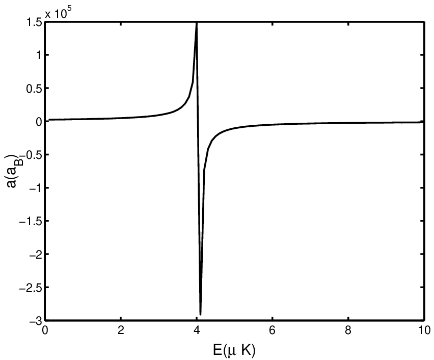
The scattering length at positive energies for the channel, calculated using a numerical solution to the radial Schrödinger equation based on the well-established 133Cs dimer potential, is shown in Fig. 3. A resonance exists at K (here and throughout, energy is measured in temperature units) due to a bound state very close to zero energy. Finding the scattering length at negative energies via equivalent numerical integration is highly unstable, as the wave function blows up in the classically forbidden region. Even if one manages to do it, it is necessary that the integration be sufficiently stable for large , well into the asymptotic region of the potential, in order to extract a meaningful scattering length tir. In addition, because we are in the neighborhood of a scattering resonance near zero energy, the strong variation of the scattering length with energy makes the requirement for a robust numerical solution even more demanding. To address these problems, we develop analytic models that will allow us to calculate the scattering matrix below threshold. In doing so, we will extend the method to a more complicated process that occurs for the multichannel scattering case.
III Analytic model
Near-threshold scattering is dominated by resonant phenomena. Such resonances can arise from a variety of different physical mechanisms, and thereby affect the form of the analytic model. We identify the nature of the resonance based on our understanding of the physical processes and the location of the poles in the -matrix. Away from resonance, the scattering properties are smooth functions and therefore can be modeled by a few free parameters. The total -matrix thus factors into resonant and background contributions,
| (4) |


For the scattering on the single channel , the resonant behaviour can arise only from a bound state or a virtual-bound state near threshold; any other type of resonance such as a Feshbach will require the inclusion of other channels. A direct numerical integration gives a bound state with a binding energy . Thus, the resonant part of the single channel -matrix can be written as jochain,
| (5) |
where , representing a pole of the -matrix in the -plane on the positive imaginary axis. There is no need to single out the other bound states, as they are energetically too far away, and their effect is absorbed in the background part. This remaining part can be written in the low energy limit as,
| (6) |
where is the background scattering length that encapsulates the effect of all other non-resonant processes, including other deeply bound states. Now we can write the complete -matrix element analytically with just one free parameter, , the value of which can be determined by fitting one positive low energy point to the equation
| (7) |
In Fig. 4 we plot the scattering phase shift as a function of the scattering energy, obtained via the full coupled channels calculation and compare it with the one obtained from Eq. (7). We see good agreement at low energy but for energies beyond 10 K a slight difference is noticed. This is expected since the linear form of the background phase shift is only valid at low energies. To remedy this problem, we use a higher order expansion for the background part given by
| (8) |
where we have added an additional free parameter, , the effective range. As before, we determine both the parameters by fitting two low energy data points. The inset of Fig. 4 shows excellent agreement of this improved model with the numerical solution.
Given the form of the S-matrix, we can predict the scattering properties in the channel at negative energy values by performing an analytic continuation of the -matrix to the imaginary -axis. From this one can consistently define the scattering length at negative energies by
| (9) |
In Fig. 5 we plot the scattering lengths obtained from the analytic procedure discussed above. These agree with the direct numerical integration just below threshold tir.
We now turn to a more complex situation: collisions between and or the channel. This is motivated by the following experimental considerations. Controlled collisions via spin-dependent transport in polarization gradient optical lattices polgradcollisions is hampered by inhomogeneous broadening arising from unwanted real or fictitious magnetic fields (due to elliptically polarized light at the atomic position) deutschandjessen. This is a particularly deleterious effect for the states that see a strongly varying difference in their optical potentials along the transport. In a lin-angle-lin optical lattice at very large detunings, atoms in the and states experience almost the same shift due to the fictitious magnetic field. Any residual broadening is due to the finite detuning effects (giving a differential scalar light shift) and the true magnetic field inhomogeneity. Controlled collisions in the channel thus offer the advantage of higher degrees of coherence, with potential applications to quantum information processing.
To treat scattering with the incoming channel, we must account for the exchange interaction, which leads to spin-changing collisions that preserve the total projection of angular momentum along a quantization axis. In this case, the -wave collisions couple the channel to the , , , and channels. At low energies, small compared to the hyperfine splitting, and are energetically closed. Moreover, in the presence of any positive magnetic field , the channel shifts to a higher energy compared to the channel, as depicted in Fig. 6. For energies that are smaller than this shift, channel is also closed. The movement of this channel from below to above the threshold can lead to a Feshbach resonance that strongly affects the scattering process, as discussed below.

The scattering phase shift for the channel is calculated by a full coupled-channels calculation. In Fig. 7 we plot as a function of scattering energy and the external magnetic field in the range of a few hundred mG. As is seen in this figure, there is a scattering resonance along the dashed line where . Also, since the resonance moves monotonically upwards in energy as a function of the field, it is clear that this resonance is a Feshbach resonance. We confirm this by calculating the bound state energy and find that it changes sign at approximately mG as shown in Fig. 8. There also exists a threshold corresponding to the opening of the channel (shown by the white solid line in Fig. 7). Across this threshold the number of open channels changes by one, as reflected in the abrupt change in the dependence of the scattering properties. This is indicated in Fig. 9 where we plot the scattering phase shift as a function of energy for various values of the field.


Based on the above understanding of the mechanisms that lead to scattering resonances, our goal is to build an analytic model that will allow us to predict the scattering lengths at negative energies where the TIR is predicted to occur. To begin with, we will again assume that the diagonal element of the matrix can be modeled as
| (10) |
where is a smooth function describing the background contribution and is the contribution arising from the Feshbach resonance. As before, the resonance leads to a pole in the -matrix. In fact it can be shown that every element of the multichannel -matrix has a pole corresponding to this resonance taylor. Also, since the location of the resonance moves upwards in energy almost linearly as a function of the field, it is fair to assume that the bound state solely resides on the channel and is shifted by an amount due to coupling to the channel. Therefore without considering the off-diagonal elements of the -matrix, the resonant part can be modeled by a pure Breit-Wigner pole,
| (11) |
so that that Feshbach contribution to the phase shift is
| (12) |
Here is the location of the bare bound state of the channel, is the width of the Feshbach resonance and represents the location of the pole of along the imaginary axis in the complex plane. This model is restricted to energies below the threshold for a finite magnetic field, . The discontinuity in the scattering phase shift seen in Fig. 9 shows that a different model is required as additional scattering channels are opened. We leave that problem for future study.


To specify our model, we need to find the parameters that characterize the Feshbach resonance, and . This is most easily done by fitting the data to the derivative of the phase shift with respect to , as determined by Eq. (12),
| (13) |
The resonance width and the location of the dressed bound state can be obtained by fitting a Lorentzian to the numerically calculated values as a function of . In Fig. 10 we plot the values obtained from this procedure. The fit to the data agrees well with the expected Wigner threshold law, , where we find . We neglect the small value of the zero intercept, typically associated with the presence of the inelastic component.
Finally, from Fig. 10 we see that for K, the level shift acquires a constant value of K. Thus, we model the scattering phase shift by
| (14) |
A more complete model at higher energies requires a determination of the threshold law for . Marcelis et al. marcelis have shown for a one channel model or more (if losses are neglected) that this law can be obtained from the below-threshold behaviour of the Feshbach bound state as a function of the field. While this is true, a direct application of their model is not possible here since we are dealing with a situation where one of the closed channel gets opened. As we are mainly interested in near-threshold behaviour in order to extract information below threshold, we will neglect the functional behaviour of at higher energies.


As in the case of channel, the background scattering length acts as a free parameter that is determined by fitting the above model to one low-energy data point. In Fig. 11 we plot the scattering phase shift for three different values of the magnetic field . The plots show a very good agreement of the analytical model to the numerical multichannel data.
Given our model, it is simple to obtain the scattering properties such as the -wave scattering length at negative energy (below threshold), by analytically continuing the above formula to the positive imaginary axis in the complex -plane. Figure 12 shows excellent agreement of the scattering lengths obtained using our model with the numerical data for positive energies. The predicted values at negative energies are also shown which agree well with the numerical value obtained just above threshold.

Critical to the use of the TIR for quantum coherent coupling between atoms is a favorable ratio of elastic to inelastic scattering processes. Near threshold scattering at energies can couple the channel to one other open channel, . Such transitions will lead to loss of the atomic pair, as the hyperfine energy will be converted to kinetic energies that are much larger than the depth of the trap. By unitarity of the -matrix, such inelastic processes imply , which can be modeled by an imaginary part of the scattering phase shift. Formal theory of multichannel threshold scattering allows us to model the energy dependence of this imaginary phase shift wigner; ross; jochain. Nesbet has shown how to separate the threshold behaviour arising from smooth background and singularities of poles such as those resulting from virtual bound states and Feshbach resonances below threshold nesbet. For a general multichannel situation consisting of open and closed channels below and above a certain threshold, the off-diagonal elements of the -matrix near threshold can be written as
| (15) |
where is some matrix, , , and is the location of the pole on the imaginary axis. In our case, for , near the channel threshold, this corresponds to one open channel and one closed channel , the relevant S-matrix element has the form
| (16) |
where is some proportionality constant that can be treated as a parameter. The imaginary part of the background phase shift is given by the Wigner threshold law where is the imaginary part of the background scattering length.
The values of the parameters of the model are typically obtained by fitting Eq. (16) to the numerical coupled channels data once the position of the pole, , is known. Marcelis et al. marcelis showed that the existence of a virtual bound state leads to a rapid change in the shift in the energy of a Feshbach resonance, in Eq. (13), and derived a simple formula that connects the pole location to the shift. From inset of Fig. 8, the rapid change in near threshold strongly indicates the existence of a such a virtual pole. We cannot, however, apply the formula in marcelis, since that analysis was limited to a two-channel model. Here, we have a more complicated interplay of three channels, (, , ), since the Feshbach resonance arises from the bound state in the channel. A more detailed analysis is required to determine the location of from first principles. Instead, since sufficient data points are available from the coupled channels numerical solution, we treat as an additional fitting parameter.

Figure 13 shows excellent fit of the above model to the numerical data. Analytic continuation of this model will give a precise determination of the off-diagonal elements of the -matrix at negative energies. This is shown in Fig. 14 for the magnetic field value G. Since the above model for the inelastic component of the -matrix is known to be valid only in a small energy region close to threshold, we have limited ourselves to the energy range to for purpose of illustration.
As a measure of the ratio of inelastic to elastic processes, we define a general energy-dependent complex scattering length,
| (17) |
which can be analytically continued to negative energies. In Fig. 14. we plot . We see that inelastic processes should not dominate, even at negative energies sufficiently far from the Feshbach resonance.
IV Summary and Conclusion
In this paper we have discussed the need for an analytic model of the -matrix in order to extract scattering properties at negative energies where numerical methods fail. Such negative energy solutions are essential for understanding trap-induced resonances that involve atoms tunneling into regions of the molecular potential that are below the threshold. Beyond improved numerical solutions, these models give us physical intuition with regards to the scattering resonances that are critical to developing many-body model Hamiltonians that can help to explain ultra-cold atomic phenomena kokkelmansandholland; servaas.
We applied this method to study the collision of two 133Cs atoms in separate harmonic traps, a situation similar to that of atoms in separate sites of a polarization gradient optical lattice. Colliding atoms in spin states that are chosen so that they are robust with respect to trapping inhomogeneities are not necessarily optimal when considering the scattering process; they can undergo multichannel scattering processes, including inelastic loss. We studied a specific example of such scattering – collisions between and . A Feshbach resonance occurs at very small magnetic fields ( 30 mG) due to coupling to a bound state in the channel. To treat this, we modeled the -matrix element via a smooth background component with an imaginary part in its scattering length and elastic single-resonance Feshbach model. The resulting total scattering length agrees well with direct numerical multichannel scattering solution at small positive energies and extends analytically to negative energies well beyond the validity of numerical solutions.
We have also discussed a model consisting of a few parameters in order to describe the off-diagonal element of -matrix that corresponds to inelastic processes. The model agrees extremely well with the coupled channels calculation at positive energies above threshold. Analytic continuation allows us to calculate the scattering length at negative energies below threshold. We note that, whereas for free space scattering the reaction rates for elastic and inelastic processes just above threshold are simply related to the complex scattering length BohnJulienne, in the negative energy case one must account for the tunneling rate from trap to the molecular potential. We will treat this in detail in a future publication.
Within the framework described in this paper, it is also possible to study the threshold behaviour arising due to the opening/closing of the channel. This particular threshold is interesting because the channel closing can be controlled by use of a very small magnetic field. Also since is the same channel that has the Feshbach bound state, opening of this channel leads to the disappearance of this Feshbach resonance. While Feshbach resonances in ultra-cold atomic gases have been thoroughly studied in recent years, our study opens up the prospect of studying Feshbach resonances in the vicinity of such tunable thresholds and their implications to the many-body properties of trapped ultra-cold gases.
We are extremely grateful to Paul Julienne for his hospitality during our visit to NIST in relation to this project and for his direction in the operation of the Mies-Julienne-Sando NIST close-coupling codes, used to perform the multichannel scattering calculations presented here. We also thank Rene Stock for helpful discussions on the trap-induced resonances. SB and IHD acknowledge financial support from the ONR, Grant No. N00014-03-1-0508, and DTO Grant No. DAAD19-13-R-0011. SB also acknowledges financial support from the W. M. Keck Program in Quantum Materials at Rice University. SK acknowledges financial support from the NWO.
References
- (1) C. A. Regal, C. Ticknor, J. L. Bohn, and D. S. Jin, Nature 424, 47 (2003); M. Greiner, C. A. Regal, and D. S. Jin, Nature 426, 537 (2003).
- (2) M. W. Zwierlein, C. A. Stan, C. H. Schunck, S. M. F. Raupach, S. Gupta, Z. Hadzibabic, and W. Ketterle, Phys. Rev. Lett. 91, 250401 (2003); K. Xu, T. Mukaiyama, J. R. Abo-Shaeer, J. K. Chin, D. Miller, and W. Ketterle, Phys. Rev. Lett. 91, 210402 (2003).
- (3) S. Jochim, M. Bartenstein, A. Altmeyer, G. Hendl, S. Riedl, C. Chin, J. Hecker Denschlag, and R. Grimm, Science 302, 2101 (2003); S. Jochim, M. Bartenstein, A. Altmeyer, G. Hendl, C. Chin, J. H. Denschlag, and R. Grimm, Phys. Rev. Lett. 91, 240402 (2003).
- (4) K. E. Strecker, G. B. Partridge and R. G. Hulet, Phys. Rev. Lett., 91, 080406 (2003).
- (5) D. Jaksch and P. Zoller, Ann. Phys. 315, 52 (2005); Immanuel Bloch J. Phys. B: At. Mol. Opt. Phys. 38 S629 (2005); M. Lewenstein em et al., Advances in Physics, 56, 243 (2007), and references therein.
- (6) S. G. Bhongale, M. R. Goosen, S. J. J. M. F. Kokkelmans, arXiv:0710.5288; S. G. Bhongale, J. N. Milstein, M. J. Holland, Phys. Rev. A 69, 053603 (2004).
- (7) U. Dorner, T. Calarco, P. Zoller, A. Browaeys, and P. Grangier, J. Opt. B 7, S341 (2005).
- (8) P. S. Jessen and I. H. Deutsch, Adv. At. Mol. Opt. Phys. 36, 91 (1996); and references therein.
- (9) C. Chin et al, Science, 305, 1128 (2004); C. A. Regal, M. Greiner, and D. S. Jin, Phys. Rev. Lett. 92, 040403 (2004); M. W. Zwierlein et al., cond-mat/0403049 (2004); T. Bourdel et al, Phys. Rev. Lett. 93, 050401 (2004); K.M. O’ Hara et al, Science 298, 2179 (2002); R. Hulet, presentation in the Quantum Gas Conference at the Kavli Institute for Theoretical Physics, Santa Barbara, CA, May 10-14 (2004).
- (10) T. Bergeman, M. G. Moore, and M. Olshanii, Phys. Rev. Lett. 91, 163201 (2003).
- (11) Moritz et al. Phy. Rev. Lett. 94, 210401 (2005). K. Winkler et al., Nature 441, 853 (2006).
- (12) D. B. M. Dickerscheid em et al. Phys. Rev. A 71, 043604 (2005). M Grupp et al. J. Phys. B: At. Mol. Opt. Phys. 40 2703 (2007). N. Nygaard, R. Piil, and K. Moelmer, unpublished, e-print arXiv:0708:2329.
- (13) R. Stock, I. H. Deutsch, and E. Bolda, Phys. Rev. Lett. 91, 183201 (2003)
- (14) R. Stock and I. H. Deutsch, Phys. Rev. A 73, 032701 (2006).
- (15) P. S. Julienne and Bo Gao, Atomic Physics 20, Proceedings of the 20th ICAP, Innsbruck, Austria (2006), e-print arXiv:physics/0609013v1.
- (16) B. Marcelis, E. G. M. van Kempen, B. J. verhaar, and S. J. J. M. F. Kokkelmans, Phys. Rev. A 70, 012701 (2004).
- (17) M. L. Chiofalo, S. J. Kokkelmans, J. N. Milstein, and M. J. Holland, Phys. Rev. Lett. 88, 090402 (2002).
- (18) Brennen et al. Phys. Rev. Lett. 82, 1060 (1999). Jaksch et al. Phys. Rev. Lett. 82, 1975 (1999). M. Greiner et al. Nature 425, 937 (2003).
- (19) P. J. Leo, C. J. Willaims, and P. S. Julienne, Phys. Rev. Lett. 85, 2721 (2000).
- (20) E. Tiesinga, E. L. Bolda, and P. S. Julienne, Phys. Rev. A 66, 013403 (2002).
- (21) C. J. Joachain in Quantum Collision Theory, North Holland, Third Edition(1983).
- (22) I. H. Deutsch and P. S. Jessen, Phys. Rev. A 57, 1972 (1998).
- (23) J. R. Taylor in Scattering Theory: The Quantum Theory of Nonrealtivistic Collisions, John Wiley and Sons, New York.
- (24) E. P. Wigner, Phys. Rev. 73, 1002 (1948).
- (25) M. H. Ross and G. L. Shaw, ann. Phys. 13, 147 (1961).
- (26) R. K. Nesbet, J. Phys. B 13, L 193 (1980).
- (27) S. J. J. M. F. Kokkelmans, J. N. Milstein, M. L. Chiofalo, R. Walser, and M. J. Holland, Phys. Rev. A 65, 053617 (2002).
- (28) John L. Bohn and P. S. Julienne, Phys. Rev. A 56 1486 (1997).