An anisotropic turbulent model for solar coronal heating

We consider a set of magnetic loops – an arcade – anchored in the photosphere and subjected to the erratic motion of convective cells. For simplicity, this arcade has a rectangular cross surface which defines the perpendicular directions and it is elongated along the longitudinal magnetic field $\mathbf{B_{0}}=B_{0}\mathbf{e_{z}}$ that defines the parallel direction as shown in Figure 3. This magnetic structure is filled by a plasma which will be modeled as an incompressible MHD fluid. In the first part of this paper, we are concerned with magnetic loops; later on we will extend our results to open magnetic field lines for which the boundary conditions will be modified. For a magnetic arcade, the boundary limits are made of two planes at altitudes $z=-\ell$ and $z=+\ell$ which are connected by the uniform magnetic field $\mathbf{B_{0}}$. Thus, the length of the loop in the longitudinal direction is $2\ell$. The cross surface is delimited as $-h<x<+h$ and $-\infty<y<+\infty$. In other words, we assume an arcade characterized by a thickness of $2h$, where $h$ is the coherence length of the magnetic field at the base of the corona, and with a large depth compare to the other length scales, with a translational invariance assumed in the $y$-direction. Note that we do

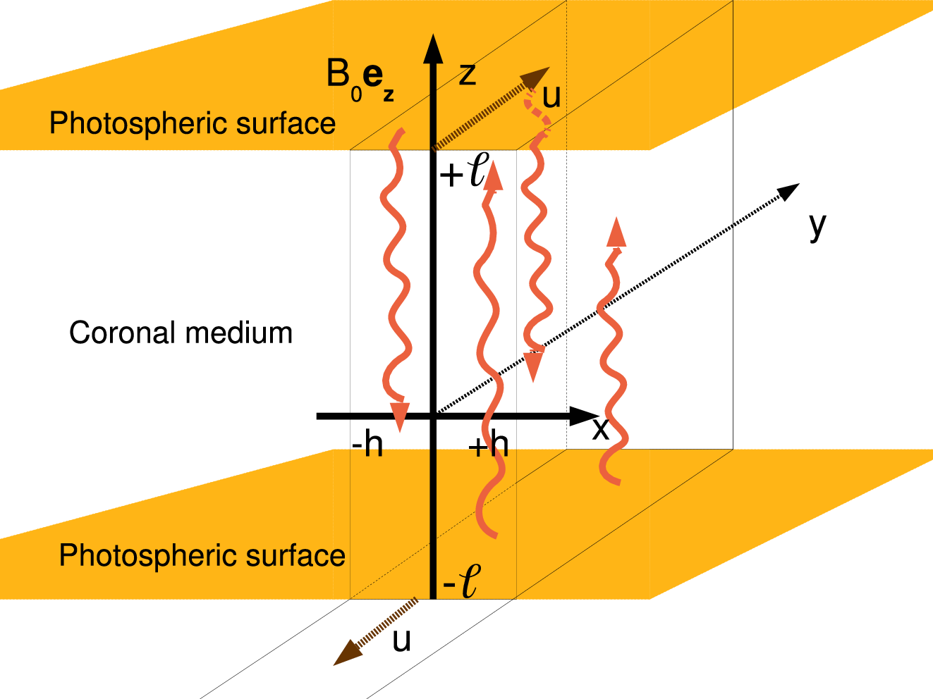
not treat the expansion of the magnetic field at the footpoint loops where $B_{0}$ has to be seen as an average value of the field at the base of the corona rather than in the photosphere itself.

The energy reservoir for the solar corona resides in the sub-photospheric convective layer. Indeed, the high-$\beta$ plasma in the photosphere constrains the magnetic field lines to be convected by the plasma flow. These motions eventually induce a shearing and a torsion of coronal magnetic field lines. The boundary motions at footpoint loops are assumed to be perpendicular and independent of the coronal plasma. More precisely, we assume for the boundary velocity field parallel to the y-axis:

This input of energy is then propagated through the coronal medium where the low-$\beta$ confines the plasma into the magnetic arcade. These boundary motions are then able to produce and maintain a state of full turbulence in the corona. Note finally the absence of mass flow through the boundaries.

The standard incompressible MHD equations are used as a first approximation to model the solar plasma, namely:

where $\mathbf{u}$ is the velocity, $\mathbf{B}$ the magnetic field (such as $\mathbf{B}=\mathbf{B_{0}}+\mathbf{b}$), $\mathbf{j}=\mathbf{\nabla}\times\mathbf{b}/\mu_{0}$ the current density (where $\mu_{0}$ is the permeability of vacuum), $\mathbf{E}$ the electric field, $\bar{\bar{\sigma}}$ the viscous stress tensor (with $\sigma_{ij}=\rho_{0}\nu(\partial u_{i}/\partial r_{j}+\partial u_{j}/\partial r_{i}))$, $\nu$ the kinematic viscosity, $\eta$ the magnetic diffusivity and $\rho_{0}$ the uniform mass density, and $P$ is the gas pressure. In the energy equation (6), the right hand side term $\mathcal{S}$ is the large-scale energy input created by the photospheric motion and $\mathcal{D}$ is the dissipation which mainly happens at the smallest scales because of, e.g., viscous and resistive effects. The left hand side term, $\mathbf{\nabla}\cdot\mathbf{\mathcal{F}}$, denotes the nonlinear transfer of total (kinetic plus magnetic) energy. (Note that all terms in equation (6) are expressed in unit volume.) Equation (7) describes how the total energy is nonlinearly transferred at different scales by velocity transport, by work due to the gas pressure, the viscous stress or the electromagnetic work due to the Poynting vector ($\mathbf{E}\times\mathbf{B}/\mu_{0}$). Other (higher order) processes like thermal conductivity which happens at microscopic scales are not considered here. Finally, equation (8) is the standard Ohm’s law which allows us to close the system.

The basic idea of this coronal model is the separation of the non-resolved inertial small-scale dynamics (see Figure 1 and 2) from the large-scale dynamics detected with current instruments. In practice, we assume that the previous MHD equations describe the large-scale behavior of the plasma; the nonlinear small-scale processes (ie. the effects of the inertial small-scales on the large-scale dynamics) will be modeled through effective dissipations, also called turbulent viscosity and resistivity. In other words, the usual molecular viscosity and magnetic resistivity are replaced by turbulent coefficients which are several orders of magnitude larger. The expression of these turbulent viscosities (hereafter denoted $\nu_{t}$ and $\eta_{t}$) will be derived in Section 3 and the MHD equations in the next Section.

An important assumption to derive this heating model is that the slow boundary motions are able to sustain a fully turbulent state in the corona, with a typical photospheric time longer than the coronal time scales. Basically, this statement means that the characteristic time of the photosphere has to be longer than the time needed for a perturbation to cross the coronal loops. For a typical longitudinal direction $\ell$ of $10^{7}$m and an Alfvén speed of several $10^{6}$m/s, one finds a crossing time of the order of 1s. For a photospheric granule with a size $\lambda=10^{6}$m and a velocity $\bar{u}=10^{3}$m/s, one finds a lifetime of about $10^{3}$s. In this case, the time scale separation is thus well satisfied. However, a validity condition may arise if the turbulent nature of the photospheric motion is taken into account since their velocities seem to follow a Kolmogorov spectrum (Roudier et al. 1987; Chou et al. 1991; Espagnet et al. 1993). Then the photospheric velocity at a given scale $\lambda$ should scale as $\lambda^{1/3}$ and the typical photospheric nonlinear time as $\lambda^{2/3}$, which decreases with the size of the granules. The associated condition is discussed and used in Section 2.8.

The nonlinear solutions of the previous MHD equations are non trivial and require direct numerical simulations on super-computers. However, we are here mainly interested in the large-scale behavior of the coronal flow which allows us to make some simplifications. We will seek solutions of the form

independent of $y$ and $t$, which satisfy, in particular, the divergence free conditions (3) and (5). These solutions do not depend on time since we assume magnetic loops maintained in a stationary regime of turbulence. We also observe that the fluctuating velocity and magnetic fields are taken perpendicular to the uniform magnetic field $\mathbf{B_{0}}$. This assumption is compatible with the fact that, in strongly magnetized media, pseudo-Alfvén waves are mainly along the uniform magnetic field whereas the nonlinear dynamics is dominated by shear-Alfvén waves in the transverse planes. We recall that shear-Alfvén and pseudo-Alfvén waves are the two kinds of linear perturbations about the equilibrium, the latter being the incompressible limit of slow magnetosonic waves. Replacing the previous solution types into the MHD equations (2) and (4) leads to

These equations describe the large-scale evolution of the plasma once the turbulent regime is established. In particular, they allow us to calculate the pressure field when the magnetic field is known. The linear form of equations (13) and (14) may be misleading since the small-scale nonlinearities are concentrated in the turbulent coefficient transports, namely the turbulent eddy viscosity $\nu_{t}$ and magnetic diffusivity $\eta_{t}$. This assumption can be justified when looking at the nonlinear evolution equations for the energy spectra, as used in Section 3. Indeed, in Fourier space, a nonlocal analysis leads to diffusive effects due to the small-scale dynamics over the large scale motions, actually stemming from absorption terms involved in the modeled energy transfers between small and large scales.

The photospheric forcing introduced in equation (1) mimics the large-scale motion of magnetic footpoints imposed by the convective cells. Following Heyvaerts & Priest 1992, we assume that the frozen-in law is satisfied in the dense photosphere which leads, when coupled with the Ohm’s law (8), to the boundary relation for the electric field:

In the close neighborhood of the photosphere, this relation is modified to take into account the magnetic diffusivity. This gives for the x-component:

The continuity of the tangential component of the electric field implies that

These photospheric conditions are of course compatible with equations (13) and (14) when $z=\pm\ell$.

The aim of this section is to express the energy flux released by photospheric motion along coronal loops. We are thus interested in the z-component of the flux (7) at the boundaries $z=\pm\ell$, namely:

The velocity boundary conditions (1) do not involve (convective) mass flows through the photospheric planes since $u_{z}(z=\pm l)=0$. Therefore, the two first terms in expression (18) do not contribute, and the input flux reduces to

with

i.e. only the viscous stress tensor and the Poynting vector contribute to the energy flux transfer to the corona. One of the main goal of this paper is to evaluate this energy flux by first solving equations (13) and (14), which depend on the turbulent viscosity and resistivity, and second, by calculating these turbulent coefficients from Alfvén wave kinetic equations.

In this section, we solve equations (13) and (14) to find the large-scale plasma behavior. We develop the x-dependence of the velocity and magnetic fields in Fourier series (since $h$ is assumed to be the coherence length of the magnetic and velocity fields in the x-direction)

where $\xi$ is either $u$ or $b$. Note that other solutions are possible with, eg. a twisted flux tube (Inverarity and Priest 1995), which do not drastically change the coronal heating predictions. Substitution of (21) into (13) and (14) gives

where $(i)$ stands for indices $(1)$ or $(2)$, and finally

Note that the magnetic field satisfies the same equation, only the boundary conditions make the distinction between the two fields. Using the following notation:

equation (24) rewrites

whose solutions may be expressed in terms of exponentials. The photospheric boundary conditions (1) and (17) combined with equation (22) gives the relations

which lead eventually to the solutions

where

The substitution of (28) into (22) and (23) gives, after some manipulations, the following expression for the magnetic field Fourier coefficients

From the solutions (28) and (30) it is now possible to calculate the energy flux (19) at footpoint levels $z=\pm\ell$. The contribution of the Poynting vector to the flux is

and the contribution of the viscous stress tensor is

The input flux coming from the photospheric boundaries ($z=\pm\ell$) is calculated by averaging over the x-periodicity of the velocity and magnetic fields (21):

After some manipulations, we obtain the total flux (from the two footpoint levels):

with $U_{n}^{2}={U^{(1)}}^{2}_{n}+{U^{(2)}}^{2}_{n}$. Note the appearance of a turbulent magnetic Prandtl number ($\nu_{t}/\eta_{t}$) whose origin is directly linked to the action of nonlinear small-scale processes on large-scales. We will later show that this number may be taken equal to unity in the Alfvén wave turbulence regime. Also note that the turbulent viscosities enter in expression (34) through the coefficients $\alpha$ and $\lambda_{n}$. The origin of the presence of $\nu_{t}$ and $\eta_{t}$ is thus due, on the one hand, to the large-scale MHD equations (13)–(14) and, on the other hand, to the Poynting vector (31) and the viscous stress tensor (32) which also include the small-scale nonlinear retroaction. The energy injected from the magnetic footpoints is propagated through the corona by Alfvén waves. Then, the collisions between ”upward” and ”downward” wave packets lead to nonlinear dynamics which is characterized by a turbulent cascade that transfers energy from the energy injection scales down to the smallest dissipative scales where energy is destroyed, and the corona heated. The coronal loops reach a stationary state of fully developed turbulence when the dissipation equals the electromagnetic and viscous stress.

The coronal heating flux is now evaluated from (34). The turbulent viscosities entering into this flux expression will be computed in the next Section. Therefore, the last unknown is the magnitude of the velocity at the photospheric boundaries (namely $U_{n}$). The goal of this section is to evaluate the scale dependence of photospheric velocities.

As reported by different measurements (Roudier et al. 1987; Chou et al. 1991; Espagnet et al. 1993), the photospheric velocities are assumed to follow a Kolmogorov isotropic spectrum

with

where $\bar{u}$ is the photospheric rms velocity, $U_{n}^{2}$ is the power spectrum of the boundary velocity fluctuations, and $k_{inj}$ is the largest scale at which energy is injected into the system; it corresponds to the size of the largest granular cells, i.e. about $1000$km. In other words, it is the integral scale of the turbulent photospheric flow from which the inertial range starts. The wave number $k_{inj}$ may be directly connected to the thickness of the arcade, such that $k_{inj}=\pi/h$. More generally, the wave number $k$ and the harmonic number $n$ may be connected through the relation $k=n\pi/h$. Converting the sum in equation (36) into an integral gives the relation

The basic idea of the model is that Alfvén wave packets interact nonlinearly along coronal magnetic structures in which the plasma is assumed to be maintained in a fully turbulent state because of the slow photospheric motion. We have seen in Section 2.2 that a condition may arise on time-scales since the photosphere is also turbulent and its typical nonlinear time, $\tau^{ph}_{nl}$, may be very short for small granules. In order to satisfy this condition, we impose that $\tau^{ph}_{nl}(\lambda)>\tau_{cross}$, where $\tau_{cross}$ is the time needed for a perturbation to cross half of the loops of length $2\ell$ at speed $B_{0}/\sqrt{\rho_{0}\mu_{0}}$, namely

and $\tau^{ph}_{nl}(\lambda)$ is the eddy turnover (nonlinear) time of granular structures at a typical scale $\lambda$ and velocity $u(\lambda)$;

This time-scale separation induces for the wave number $k=2\pi/\lambda$, the inequality $k<k_{cross}$, where

Hence, the upper limit of the summation on harmonic numbers in (34) is given by $N_{cross}$ which is a large number since the Alfvén velocity is much larger than the photospheric rms velocity. For that reason, the expression (34) may also be written as an integral with

The energy injection produced by the photospheric motion is finally rewritten as follows:

with

Under the time-scale condition discussed above, the coronal structure is submitted to slow external forcing. Note that other time scales are present in our problem; namely, the nonlinear coronal time, $\tau_{nl}$, and the Alfvén time, $\tau_{A}$, which has nothing to do with the crossing time $\tau_{cross}$ introduced above. It may be interpreted as the time of interaction between two counter-propagating Alfvén wave packets. Both times will be used in Section 3 where the nonlinear small-scale dynamics will be analyzed. The main assumption made in such wave turbulence dynamics is that the Alfvén time is smaller than the nonlinear coronal time. Note that in MHD the transfer time-scale is built on $\tau_{nl}$ and $\tau_{A}$ which makes a great difference in Navier-Stokes fluids for which the transfer time is the nonlinear time. This point will be further discussed in the next section. Then the following hierarchy of times may be estimated

As seen in Section 2.2, the nonlinear photospheric time can be as large as $10^{3}$s and the crossing time is about $1$s. For the two other characteristic time scales, no observational constraints can be used. However, recent direct numerical simulations (Bigot et al. 2008b) show clearly that a turbulent MHD flow evolving in a strong uniform magnetic field ($B_{0}>b$) exhibits a time ratio $\tau_{A}/\tau_{nl}<1$, which decreases as the strength of the uniform field increases.

The first description of incompressible MHD turbulence proposed by Iroshnikov and Kraichnan (IK) in the 1960s (Iroshnikov 1964; Kraichnan 1965) is based on a modified version of the Kolmogorov dimensional analysis where the large-scale magnetic effects are taken into account although the fluid is supposed to be globally isotropic. The IK’s heuristic model includes Alfvén waves which approximate the magnetic field at the largest scales as a uniform magnetic field. Then, it is the sporadic and successive collisions between counterpropagating Alfvén waves that produce the turbulent cascade. At leading order, the nonlinear dynamics is driven by three wave interactions, and the transfer time through the scales is estimated by $\tau_{tr}\sim\tau_{nl}^{2}/\tau_{A}$, where $\tau_{nl}\sim\lambda/u_{\lambda}$ is the nonlinear turnover time whereas $\tau_{A}\sim\lambda/{\tilde{B}_{0}}$ is the Alfvén wave period (where $\tilde{B}_{0}$ stands for the Alfvén speed, taken as the rms magnetic field fluctuation). Hence, the energy spectrum is $k^{-3/2}$.

The weakness of the IK phenomenology is the apparent contradiction between the presence of Alfvén waves and the absence of a strong uniform magnetic field. This point and the role of a strong external magnetic field $\mathbf{B_{0}}$ have been widely discussed in the literature, in particular during the last two decades (Strauss 1976, Montgomery & Turner 1981; Shebalin et al. 1983; Oughton et al. 1994; Goldreich & Sridhar 1995; Ng & Bhattacharjee 1996; Matthaeus et al. 1998; Galtier et al. 2000; Nazarenko et al., 2001; Milano et al. 2001; Chandran 2005; Bigot et al. 2008a). One of the most clearly established results is the bi-dimensionalization of a turbulent flow with a strong reduction of the nonlinear transfers along the $\mathbf{B_{0}}$ ambiant field.

In the case of coronal structures, like magnetic arcades or open magnetic fields in coronal holes, a strong magnetic field at large-scale is clearly present. This field is often modeled as a uniform field through, for example, the approximation of reduced MHD (see, e.g., Dmitruk & Matthaeus 2003; Buchlin et al. 2007). It was thought until recently (see eg. Oughton et al. 2004) that the reduced MHD approximation was only able to describe the regime of strong turbulence but a recent work (Nazarenko 2007) has extended its domain of application to the wave turbulence regime as well. This point is particularly important for our model which is based on the latter regime. In our model, the magnetic arcade is composed of a network of parallel strands that are maintained in a fully developed turbulent regime. Contrary to the isotropy hypothesis originally assumed by Heyvaerts & Priest 1992, we include anisotropic effects through turbulent viscosities. In this approach, it is thus necessary to distinguish between the perpendicular ($\perp$) and parallel ($\parallel$) directions to the uniform $\mathbf{B_{0}}$ field.

An important anisotropic property discussed in the literature (Higdon 1984; Goldreich & Sridhar 1995; Galtier et al. 2005; Boldyrev 2006) is the interdependence of perpendicular and parallel scales. According to direct numerical simulations (see, e.g., Cho & Vishniac 2000; Maron & Goldreich 2001; Shaikh & Zank 2007; Bigot et al. 2008b), one of the most fundamental results seems to be the (critical) balance between the nonlinear and Alfvén times which leads to the scaling relation $k_{\parallel}\sim k^{2/3}_{\perp}$. In other words, a turbulent MHD flow evolving in a strongly magnetized medium seems to be characterized by an approximately constant ratio (generally smaller than one) between the Alfvén and the nonlinear times. This result (generally) implies a dynamics mainly driven by Alfvén wave interactions.

The incompressible MHD equations (2)–(5) may be reformulated in terms of the Elsässer fluctuations

with magnetic fields written in velocity units ($\mathbf{\tilde{b}}=\mathbf{b}/\sqrt{\mu_{0}\rho_{0}}$), and in the inviscid case (ie. in the absence of the dissipative terms proportional to the kinematic viscosity and the magnetic diffusivity),

Here, $s=\pm$, stands for the directional polarity, indicating the propagating direction of waves along $\mathbf{\tilde{B}_{0}}=\mathbf{B_{0}}/\sqrt{\mu_{0}\rho_{0}}$; $P_{*}$ is the total (kinetic plus magnetic) pressure. Note that the present analysis is focused on the nonlinear plasma dynamics from which the turbulent transport coefficients will be derived. In the presence of a strong uniform magnetic field, MHD turbulence may be dominated by wave dynamics for which the nonlinearities are weak, and thus $\tau_{A}\ll\tau_{nl}$. In this limit, a small formal parameter $\epsilon$ can be introduced to measure the strength of the nonlinearities to give, for the jth-component

(with Einstein’s notation used for indices). Note that the parallel direction ($\parallel$) corresponds to the z-direction.

We will Fourier transform such equations, with the following definitions for the Fourier transform of the Elsässer field components $z^{s}_{j}(\mathbf{x},t)$:

where $\omega_{k}={\tilde{B}_{0}}k_{\parallel}$ is the Alfvén frequency. The quantity $a^{s}_{j}(\mathbf{k},t)$ is the wave amplitude in the interaction representation, hence the factor $e^{is\omega_{k}t}$. The Fourier transform of equation (48) thus is

Here, $P_{jn}$ is the projector on solenoidal vectors such that $P_{jn}(\textbf{k})=\delta_{jn}-k_{j}k_{n}/k^{2}$; $\delta_{\mathbf{k},\mathbf{\kappa}\mathbf{L}}=\delta(\mathbf{k}-\mathchoice{\kern-0.2pt\hbox{$\displaystyle\kappa$}\kern-5.76158pt\kern 0.4pt\hbox{$\displaystyle\kappa$}\kern-5.76158pt\kern-0.2pt\raise 0.3pt\hbox{$\displaystyle\kappa$}}{\kern-0.2pt\hbox{$\textstyle\kappa$}\kern-5.76158pt\kern 0.4pt\hbox{$\textstyle\kappa$}\kern-5.76158pt\kern-0.2pt\raise 0.3pt\hbox{$\textstyle\kappa$}}{\kern-0.2pt\hbox{$\scriptstyle\kappa$}\kern-4.68175pt\kern 0.4pt\hbox{$\scriptstyle\kappa$}\kern-4.68175pt\kern-0.2pt\raise 0.3pt\hbox{$\scriptstyle\kappa$}}{\kern-0.2pt\hbox{$\scriptscriptstyle\kappa$}\kern-4.13779pt\kern 0.4pt\hbox{$\scriptscriptstyle\kappa$}\kern-4.13779pt\kern-0.2pt\raise 0.3pt\hbox{$\scriptscriptstyle\kappa$}}-\mathbf{L})$ reflects the triadic interaction, and $\Delta\omega=\omega_{L}-\omega_{k}-\omega_{\kappa}$ is the frequency mixing. The appearance of an integration over wave vectors $\textstyle\kappa$$\textstyle\kappa$$\textstyle\kappa$ and $\mathbf{L}$ is directly linked to the quadratic nonlinearity of equation (48) (as a result of the Fourier transform of a correlation product).

Equation (50) is the compact expression of the incompressible MHD equations when a strong uniform magnetic is present. It is the point of departure of the wave turbulence formalism which consists of writing equations for the long time behavior of second order moments. In such an asymptotic and statistical development, the time-scale separation, $\tau_{A}/\tau_{nl}\ll 1$, leads to the destruction of some nonlinear terms, including the fourth order cumulants, and only the resonance terms survive (Galtier et al. 2000; Galtier et al. 2002). It allows one to obtain a natural asymptotic closure for the moment equations. In such a statistical development, the following general definition for the total (shear- plus pseudo-Alfvén wave) energy spectrum is used;

where $\langle\rangle$ stands for ensemble average and $k_{\perp}=|\mathbf{k_{\perp}}|$. In absence of helicities and in the case of an axially symmetric turbulence, the asymptotic equations simplify. For the shear-Alfvén waves, the energy spectrum is given by

where $f(k_{\parallel})$ is a function fixed by the initial conditions (ie. there is no energy transfer along the parallel direction). The transverse part obeys the following nonlinear equation (the small parameter $\epsilon$ is now included in the time variable)

where $\phi$ is the angle between $\mathbf{k_{\perp}}$ and $\mathbf{L_{\perp}}$, and $\theta$ is the angle between $\mathbf{k_{\perp}}$ and $\mathchoice{\kern-0.2pt\hbox{$\displaystyle\kappa$}\kern-5.76158pt\kern 0.4pt\hbox{$\displaystyle\kappa$}\kern-5.76158pt\kern-0.2pt\raise 0.3pt\hbox{$\displaystyle\kappa$}}{\kern-0.2pt\hbox{$\textstyle\kappa$}\kern-5.76158pt\kern 0.4pt\hbox{$\textstyle\kappa$}\kern-5.76158pt\kern-0.2pt\raise 0.3pt\hbox{$\textstyle\kappa$}}{\kern-0.2pt\hbox{$\scriptstyle\kappa$}\kern-4.68175pt\kern 0.4pt\hbox{$\scriptstyle\kappa$}\kern-4.68175pt\kern-0.2pt\raise 0.3pt\hbox{$\scriptstyle\kappa$}}{\kern-0.2pt\hbox{$\scriptscriptstyle\kappa$}\kern-4.13779pt\kern 0.4pt\hbox{$\scriptscriptstyle\kappa$}\kern-4.13779pt\kern-0.2pt\raise 0.3pt\hbox{$\scriptscriptstyle\kappa$}}_{\perp}$ with the perpendicular wave vectors satisfying the triangular relation $\mathbf{k_{\perp}}=\mathbf{L_{\perp}}+\mathchoice{\kern-0.2pt\hbox{$\displaystyle\kappa$}\kern-5.76158pt\kern 0.4pt\hbox{$\displaystyle\kappa$}\kern-5.76158pt\kern-0.2pt\raise 0.3pt\hbox{$\displaystyle\kappa$}}{\kern-0.2pt\hbox{$\textstyle\kappa$}\kern-5.76158pt\kern 0.4pt\hbox{$\textstyle\kappa$}\kern-5.76158pt\kern-0.2pt\raise 0.3pt\hbox{$\textstyle\kappa$}}{\kern-0.2pt\hbox{$\scriptstyle\kappa$}\kern-4.68175pt\kern 0.4pt\hbox{$\scriptstyle\kappa$}\kern-4.68175pt\kern-0.2pt\raise 0.3pt\hbox{$\scriptstyle\kappa$}}{\kern-0.2pt\hbox{$\scriptscriptstyle\kappa$}\kern-4.13779pt\kern 0.4pt\hbox{$\scriptscriptstyle\kappa$}\kern-4.13779pt\kern-0.2pt\raise 0.3pt\hbox{$\scriptscriptstyle\kappa$}}_{\perp}$ (see Figure 4). Note that from the axisymmetric assumption, the azimuthal angle integration has already been performed, and we are only left with an integration over the absolute values of the two wave numbers, $\kappa_{\perp}=|\mathchoice{\kern-0.2pt\hbox{$\displaystyle\kappa$}\kern-5.76158pt\kern 0.4pt\hbox{$\displaystyle\kappa$}\kern-5.76158pt\kern-0.2pt\raise 0.3pt\hbox{$\displaystyle\kappa$}}{\kern-0.2pt\hbox{$\textstyle\kappa$}\kern-5.76158pt\kern 0.4pt\hbox{$\textstyle\kappa$}\kern-5.76158pt\kern-0.2pt\raise 0.3pt\hbox{$\textstyle\kappa$}}{\kern-0.2pt\hbox{$\scriptstyle\kappa$}\kern-4.68175pt\kern 0.4pt\hbox{$\scriptstyle\kappa$}\kern-4.68175pt\kern-0.2pt\raise 0.3pt\hbox{$\scriptstyle\kappa$}}{\kern-0.2pt\hbox{$\scriptscriptstyle\kappa$}\kern-4.13779pt\kern 0.4pt\hbox{$\scriptscriptstyle\kappa$}\kern-4.13779pt\kern-0.2pt\raise 0.3pt\hbox{$\scriptscriptstyle\kappa$}}_{\perp}|$ and $L_{\perp}=|\mathbf{L_{\perp}}|$. In the same way, equations can be written for pseudo-Alfvén waves which are passively advected by shear-Alfvén waves, namely

with by definition

where ${\tilde{f}}(k_{\parallel})$ is a function fixed by the initial condition. Equations (53) and (54) – called wave kinetic equations – only involve perpendicular nonlinear dynamics (with a dependence only on the perpendicular components of the wave vectors), a situation expected from previous works (Strauss 1976, Montgomery & Turner 1981; Shebalin et al. 1983; Oughton et al. 1994; Goldreich & Sridhar 1995; Ng & Bhattacharjee 1996; Matthaeus et al. 1998) that showed the decrease of the parallel nonlinear transfers with the increasing strength of the external magnetic field $\mathbf{\tilde{B}_{0}}$.

The main goal of this Section is the derivation of turbulent viscosities in the context of strongly anisotropic MHD turbulence. We have seen that wave turbulence leads to the inhibition of nonlinear transfers in the $\mathbf{\tilde{B}_{0}}$ direction, and to the bidimensional reduction of the dynamics. This result makes a strong difference to purely isotropic MHD turbulence from which the turbulent viscosities were derived in the original model (Heyvaerts & Priest 1992). We believe that taking into account the flow anisotropy is an important improvement in the description of the coronal heating problem.

The wave kinetic equations are assumed to describe the nonlinear dynamics at small inertial scales. These scales correspond to the scales unresolved by the current spacecrafts which are reported in Figure 1. The turbulent viscosities represent the average effect of nonlinearities at these small scales, and they appear in the large-scale equations (13)–(14). In practice, we make a Taylor expansion of the wave kinetic equations for nonlocal triadic interactions (Pouquet et al. 1976) that satisfy the relation

which leads to

for triadic interactions $\mathbf{k}_{\perp}=\mathchoice{\kern-0.2pt\hbox{$\displaystyle\kappa$}\kern-5.76158pt\kern 0.4pt\hbox{$\displaystyle\kappa$}\kern-5.76158pt\kern-0.2pt\raise 0.3pt\hbox{$\displaystyle\kappa$}}{\kern-0.2pt\hbox{$\textstyle\kappa$}\kern-5.76158pt\kern 0.4pt\hbox{$\textstyle\kappa$}\kern-5.76158pt\kern-0.2pt\raise 0.3pt\hbox{$\textstyle\kappa$}}{\kern-0.2pt\hbox{$\scriptstyle\kappa$}\kern-4.68175pt\kern 0.4pt\hbox{$\scriptstyle\kappa$}\kern-4.68175pt\kern-0.2pt\raise 0.3pt\hbox{$\scriptstyle\kappa$}}{\kern-0.2pt\hbox{$\scriptscriptstyle\kappa$}\kern-4.13779pt\kern 0.4pt\hbox{$\scriptscriptstyle\kappa$}\kern-4.13779pt\kern-0.2pt\raise 0.3pt\hbox{$\scriptscriptstyle\kappa$}}_{\perp}+\mathbf{L}_{\perp}$ (see Figure 4). Then, relation (57) is substituted into the kinetic equations (53)-(54) for, respectively, the shear-Alfvén waves

and the pseudo-Alfvén waves

Finally, we obtain:

where $\nu_{\perp}^{s}$ and $\nu_{\parallel}^{s}$ are the so-called turbulent viscosities, corresponding respectively to shear- and pseudo-Alfvén waves, defined as

The turbulent viscosities are thus directly obtained after integration over the $\theta$ angle. Note that, similarly to the original paper (Heyvaerts & Priest 1992), the integration is made from the beginning of the inertial range (at $\kappa_{inj}$) where the injection of energy is made; this choice contrasts with some models where a wavenumber cut-off is chosen inside the inertial range which gives a k-dependence of the turbulence viscosity (see eg. Bærenzung et al. 2008). An evaluation of the turbulent viscosities is now possible by the use of the exact power law solutions of the integro-differential equations (53) and (54). This is first made in the context of a magnetic arcade for which the inward and outward Alfvén waves are exactly balanced (balanced case). This approach is then generalized to open magnetic fields for which outward Alfvén waves are dominant (unbalanced case).

For balanced turbulence, as said before, it is not necessary to distinguish outward from inward Alfvén waves. We thus drop the directional polarity $s$, and we obtain

In this case, the exact power law solution of equation (53) is (Galtier et al. 2000)

where $C_{K}$ is the Kolmogorov constant whose value is about $0.585$, and $P_{\perp}$ is the constant energy flux of shear-Alfvén waves whose definition is

It is important to note that it is the condition of constant energy flux that allows to find (by the Zakharov transformation) the exact power law solution of the nonlinear wave turbulence equation. The introduction of (66) into (64) and (65) gives

Note the relation $\nu_{\parallel}=4\nu_{\perp}$ between the turbulent coefficients corresponding to pseudo- and shear-Alfvén waves. In particular, this means that the pseudo-Alfvén wave energy is susceptible to decay faster than the shear-Alfvén one. Actually, this property has been detected recently in numerical simulations of freely decaying MHD turbulence (Bigot et al. 2008a). Finally note that in this wave turbulence regime, there is an automatic equipartition state between the kinetic and magnetic energies. Therefore, no distinction will be made between the average nonlinear effects acting on the velocity and on the magnetic field. A unit turbulent magnetic Prandtl number will then be taken (ie. $\nu_{t}/\eta_{t}=1$).

The magnetic arcade being supposed in a fully turbulent state, the energy transfer rate is then assumed to be constant at each scales in the inertial range, from the largest photospheric scales at which energy is injected, down to the small dissipative scale fom which heating starts to occur. This fundamental remark allows us to link the first estimate of the energy flux (42), based on the photospheric motions, to the flux through the anisotropic arcade scales, estimated from the turbulent eddy viscosity and magnetic diffusivity.

According to relations (52) and (67) the energy flux $P_{\perp}$, introduced above, satisfies the general relation

We remind that $f$ is an arbitrary dimensionless function which reflects the absence of nonlinear transfers along the $\mathbf{\tilde{B}_{0}}$ direction. The coronal heating in a fraction of the arcade, say $Q$, can thus be estimated from the small-scale dynamics by

where $L$ delimits a fraction of the arcade thickness in the y-direction and $Q$ is measured in Js^-1 (Note the presence of the constant mass density). In the same manner, we may evaluate the coronal heating from the large-scale energy flux ${|\mathcal{F}_{z}|}$. It gives for the same coronal volume:

Hence, the relation between both photospheric and turbulent fluxes:

The small-scale analysis gives two turbulent viscosities coming from, respectively, the shear- and pseudo-Alfvén wave energy. To be consistent with our model, we will only consider the former one since, in the strongly anisotropic limit of wave turbulence, the pseudo-Alfvén waves fluctuate only in the parallel direction to the ambiant magnetic field. However, we note that the inclusion of the pseudo waves effect modifies only slightly the form of the turbulent viscosity (by a factor $5$). Then, relation (73) gives (with $\nu_{t}\equiv\nu_{\perp}$)

Together with the injection wave number $\kappa_{inj}=\pi/h$, related to the arcade thickness, we obtain

The substitution of (42) into (75) leads to the relation

where a unit turbulent magnetic Prandtl number is taken ($\nu_{t}=\eta_{t}$). The above expression also gives

where

In the next section, we use the following approximation:

According to the specific value of the $k$ wave number, different estimates may be made for the function $\Psi(k)$ that enters in the expression (42) of the energy injection by photospheric velocities, namely

We recall that $\alpha=B_{0}/\sqrt{\mu_{0}\rho_{0}\nu_{t}\eta_{t}}={\tilde{B}_{0}}/\nu_{t}$; it is therefore a way to measure, for example, the relative importance of the diffusive terms in equations (13) and (14) which can be rewritten as