A New Outer Bound and the Noisy-Interference Sum-Rate Capacity for Gaussian Interference Channels

The following is a new outer bound on the capacity region of Gaussian ICs.

Remark 1: The bounds (1)-(3) are obtained by providing different genie-aided signals to the receivers. There is overlap of the range of $\mu$, $\eta_{1}$, and $\eta_{2}$, and none of the bounds uniformly dominates the other two bounds. Which one of them is active depends on the channel conditions and the rate pair.

Remark 2: Equations (2) and (3) are outer bounds for the capacity region of a Z-IC, and a Z-IC is equivalent to a degraded IC [5]. For such channels, it can be shown that (2) and (3) are the same as the outer bounds in [14]. For $0\leq\eta_{1}\leq\frac{1+bP_{1}}{b+bP_{1}}$ and $\eta_{2}\geq\frac{a+aP_{2}}{1+aP_{2}}$, the bounds in (2) and (3) are tight for a Z-IC (or degraded IC) because there is no power sharing between the transmitters. Consequently, $\frac{1+bP_{1}}{b+bP_{1}}$ and $\frac{a+aP_{2}}{1+aP_{2}}$ are the negative slopes of the tangent lines for the capacity region at the corner points.

Remark 3: The bounds in (2)-(3) turn out to be the same as the bounds in [10, Theorem 2]. We show this by proving that (3) is equivalent to [10, page 584, (37)-(38)] but with equalities rather than inequalities. Consider the rates

	$\displaystyle R_{1}$	$\displaystyle=$	$\displaystyle\frac{1}{2}\log\left(1+\frac{P_{1}^{\prime}}{P_{2}^{\prime}+1/a}\right)$		(17)
	$\displaystyle R_{2}$	$\displaystyle=$	$\displaystyle\frac{1}{2}\log\left(1+P_{2}^{\prime}\right)$		(18)
	$\displaystyle P_{1}^{\prime}+P_{2}^{\prime}$	$\displaystyle=$	$\displaystyle\frac{P_{1}}{a}+P_{2}$		(19)

for $0\leq P_{1}^{\prime}\leq P_{1}$. We rewrite (17) and (18) in the form of the weighted sum

$\displaystyle R_{1}+\alpha R_{2}=\frac{1}{2}\log\left(1+\frac{P_{1}^{\prime}}{P_{2}^{\prime}+1/a}\right)+\frac{\alpha}{2}\log\left(1+P_{2}^{\prime}\right).$

(20)

Observe that (20) represents a line with slope $\alpha$ where

	$\displaystyle\alpha$	$\displaystyle=$	$\displaystyle-\frac{\partial R_{1}}{\partial R_{2}}$		(21)
		$\displaystyle=$	$\displaystyle-\frac{\partial R_{1}}{\partial P_{2}^{\prime}}\left/\frac{\partial R_{2}}{\partial P_{2}^{\prime}}\right.$
		$\displaystyle=$	$\displaystyle-\frac{\partial\log\left(1+\frac{P_{1}/a+P_{2}-P_{2}^{\prime}}{P_{2}^{\prime}+1/a}\right)}{\partial P_{2}^{\prime}}\left/\frac{\partial\log\left(1+P_{2}^{\prime}\right)}{\partial P_{2}^{\prime}}\right.$
		$\displaystyle=$	$\displaystyle\frac{a+aP_{2}^{\prime}}{1+aP_{2}^{\prime}}.$

We thus obtain

$\displaystyle P_{2}^{\prime}=\frac{a-\alpha}{a\alpha-a}.$

(22)

Substituting (22) into (20), we have

$\displaystyle R_{1}+\alpha R_{2}=\frac{1}{2}\log\left(1+P_{1}+aP_{2}\right)-\frac{1}{2}\log\left(1+\frac{a-\alpha}{\alpha-1}\right)+\frac{\alpha}{2}\log\left(1+\frac{a-\alpha}{a\alpha-a}\right),$

which is the same as (3). The relation $a\leq\alpha\leq\frac{a+aP_{2}}{1+aP_{2}}$ follows from (21) and $0\leq P_{2}^{\prime}\leq P_{2}$.

Remark 4: The bounds in [10, Theorem 2] are obtained by getting rid of one of the interference links to reduce the IC into a Z interference channel (or Z-IC, see [5]). Next, the proof in [10] allowed the transmitters to share their power, which further reduces the Z-IC into a degraded broadcast channel. Then the capacity region of this degraded broadcast channel is an outer bound for the capacity region of the original IC. The bounds in (2) and (3) are also obtained by reducing the IC to a Z-IC. Although we do not explicitly allow the transmitters to share their power, it is interesting that these bounds are equivalent to the bounds in [10, Theorem 2] with power sharing. In fact, a careful examination of our new derivation reveals that power sharing is implicitly assumed. For example, for the term $h\left(X_{1}^{n}+Z_{1}^{n}\right)-\eta_{1}h\left(\sqrt{b}X_{1}^{n}+Z_{2}^{n}\right)$ of (57) below, user $1$ uses power $P_{1}^{*}=\frac{b\eta_{1}-1}{b-b\eta_{1}}\leq P_{1}$ , while for the term $\eta_{1}h\left(Y_{2}^{n}\right)$ user $1$ uses all the power $P_{1}$. This is equivalent to letting user $1$ use the power $P_{1}^{*}$ for both terms, and letting user $2$ use a power that exceeds $P_{2}$. To see this, consider (57) below and write

	$\displaystyle n(R_{1}+\eta_{1}R_{2})$	$\displaystyle\leq$	$\displaystyle\frac{n}{2}\log\left(P_{1}^{*}+1\right)-\frac{n\eta_{1}}{2}\log\left(bP_{1}^{*}+1\right)+\frac{n\eta_{1}}{2}\log\left(1+bP_{1}+P_{2}\right)+n\epsilon$
		$\displaystyle=$	$\displaystyle\frac{n}{2}\log\left(P_{1}^{*}+1\right)-\frac{n\eta_{1}}{2}\log\left(bP_{1}^{*}+1\right)+\frac{n\eta_{1}}{2}\log\left(1+bP_{1}^{*}+P_{2}+b(P_{1}-P_{1}^{*})\right)+n\epsilon$
		$\displaystyle=$	$\displaystyle\frac{n}{2}\log\left(P_{1}^{\prime}+1\right)-\frac{n\eta_{1}}{2}\log\left(bP_{1}^{\prime}+1\right)+\frac{n\eta_{1}}{2}\log\left(1+bP_{1}^{\prime}+P_{2}^{\prime}\right)+n\epsilon,$

where $P_{1}^{\prime}\triangleq P_{1}^{*}$, and $P_{2}^{\prime}\triangleq P_{2}+b(P_{1}-P_{1}^{*})$. Therefore, one can assume that user $2$ uses extra power provided by user $1$.

Remark 5: Theorem 1 improves [11, Theorem 3]. Specifically, for the three sum-rate bounds of [11, Theorem 3], the first bound can be obtained from (57) with $P_{1}^{*}=P_{1}$ in (III-A). Therefore, the bound in (2) is tighter than the first sum-rate bound of [11, Theorem 3]. Similarly, the bound in (3) is tighter than the second sum-rate bound of [11, Theorem 3]. The third sum-rate bound in [11, Theorem 3] is a special case of (1) with $\sigma_{1}^{2}=\frac{1}{b},\sigma_{2}^{2}=\frac{1}{a},\rho_{1}=\rho_{2}=0$.

Remark 6: Our outer bound is not always tighter than that of [11] for all rate points. The reason is that in [11, last two equations of (39)], different genie-aided signals are provided to the same receiver. Our outer bound can also be improved in a similar and more general way by providing different genie-aided signals to the receivers. Specifically the starting point of the bound is

$\displaystyle n\left(R_{1}+\mu R_{2}\right)\leq\sum_{i=1}^{k}\lambda_{i}I\left(X_{1}^{n};Y_{1}^{n},U_{i}\right)+\sum_{j=1}^{m}\mu_{i}I\left(X_{2}^{n};Y_{2}^{n},W_{j}\right)+n\epsilon,$

(23)

where $\sum_{i=1}^{k}\lambda_{i}=1,\sum_{j=1}^{m}\mu_{j}=\mu,\lambda_{i}>0,\mu_{j}>0$.

The outer bound in Theorem 1 is in the form of an optimization problem. Four parameters $\rho_{1},\rho_{2},\sigma_{1}^{2},\sigma_{2}^{2}$ need to be optimized for different choices of the weights $\mu,\eta_{1},\eta_{2}$. When $\mu=1$, Theorem 1 leads directly to the following sum-rate capacity result.

Remark 7: The sum-rate capacity for a Z-IC with $a=0$, $0<b<1$ is a special case of Theorem 2 since (24) is satisfied. The sum capacity is therefore given by (25).

Theorem 2 follows directly from Theorem 1 with $\mu=1$. It is remarkable that a genie-aided bound is tight if (24) is satisfied since the genie provides extra signals to the receivers without increasing the rates. This situation is reminiscent of the recent capacity results for vector Gaussian broadcast channels (see [15]). Furthermore, the sum-rate capacity (25) is achieved by treating the interference as noise. We therefore refer to channels satisfying (24) as ICs with noisy interference. Note that (24) involves both channel gains $a,b$ and both powers $P_{1}$ and $P_{2}$. The constraint (24) implies that

$\displaystyle\sqrt{a}+\sqrt{b}\leq 1.$

(26)

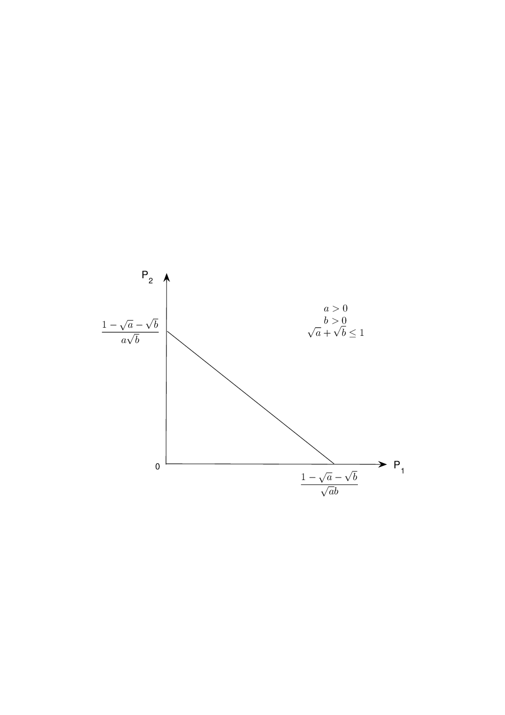
Moreover, as shown in Fig. 1, the powers $P_{1}$ and $P_{2}$ must be inside the triangle defined by:

	$\displaystyle P_{1}$	$\displaystyle\geq$	$\displaystyle 0,$
	$\displaystyle P_{2}$	$\displaystyle\geq$	$\displaystyle 0,$
	$\displaystyle b\sqrt{a}P_{1}+a\sqrt{b}P_{2}$	$\displaystyle\leq$	$\displaystyle 1-\sqrt{a}-\sqrt{b}.$		(27)

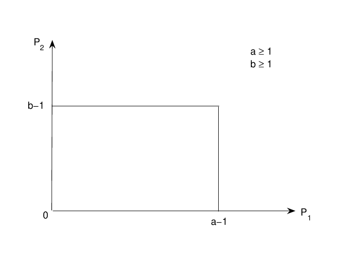
These constraints can be considered as a counterpart of the IC with very strong interference [2] whose powers should be inside the rectangle defined in Fig. 2:

	$\displaystyle a>1,b>1,$
	$\displaystyle 0\leq P_{1}\leq a-1,$
	$\displaystyle 0\leq P_{2}\leq b-1.$

The ICs with noisy interference and ICs with very strong interference are two extreme cases in terms of the decoding strategy to achieve the sum-rate capacity. In the former case, the sum-rate capacity is achieved by treating interference as noise, while in the latter case, the interference is decoded before, or together with, the intended messages.

For symmetric Gaussian ICs with $a=b$ and $P_{1}=P_{2}$, the conditions in (26) and (27) become

	$\displaystyle a=b$	$\displaystyle\leq$	$\displaystyle\frac{1}{4},$		(28)
	$\displaystyle P_{1}=P_{2}=P$	$\displaystyle\leq$	$\displaystyle\frac{\sqrt{a}-2a}{2a^{2}}.$		(29)

“Noisy interference” is therefore “weaker” than “weak interference” as defined in [5] and [16], namely $a\leq\frac{\sqrt{1+2P}-1}{2P}$ or

$\displaystyle P\leq\frac{1-2a}{a^{2}}.$

(30)

Recall that [16] showed that for “weak interference” satisfying (30), treating interference as noise achieves larger sum rate than time-or frequency-division multiplexing (TDM/FDM), and [5] claimed that in “weak interference” the largest known achievable sum rate is achieved by treating the interference as noise.

Under the constraint (32), we have the following inequality:

$\displaystyle\frac{1}{2}\log\left(1+\frac{P_{2}}{1+bP_{1}}\right)\leq\frac{1}{2}\log\left(1+\frac{aP_{2}}{1+P_{1}}\right).$

(33)

Therefore, the sum-rate capacity is achieved by a simple scheme: user $1$ transmits at the maximum rate and user $2$ transmits at the rate that both receivers can decode its message with single-user detection. Observe further that this rate pair permits $R_{2}=\frac{1}{2}\log\left(1+\frac{aP_{2}}{1+P_{1}}\right)$ when $R_{1}$ reaches its maximum. Such a rate constraint was considered in [5, Theorem 1] which established a corner point of the capacity region. However it was pointed out in [16] that the proof in [5] was flawed. Theorem 3 shows that the rate pair of [16] is in fact a corner point of the capacity region when $a>1,0<b<1$ and (32) is satisfied, and this rate pair achieves the sum-rate capacity.

The sum-rate capacity of the degraded IC $(ab=1,0<b<1)$ is a special case of Theorem 3. Besides this example, there are two other kinds of ICs to which Theorem 3 applies. The first case is $ab>1$. In this case, $P_{1}$ can be any positive value. The second case is $ab<1$ and $P_{1}\leq\frac{a-1}{1-ab}$. For both cases, the signals from user $2$ can be decoded first at both receivers.

We reiterate that both Theorems 2 and 3 are direct results of Theorem 1, and Theorem 1 is derived by having a genie provide extra information to the receivers. We summarize the sum-rate capacity for Gaussian ICs from Theorems 2 and 3 and previous results in [2, 4, 3]. In Fig. 3, four curves $ab=1$, $a=1$, $b=1$, and $\sqrt{a}+\sqrt{b}\leq 1$ divide channel gain plane into $7$ regimes. The sum-rate capacity for each regime under certain power constraints is shown in Tab. I.

Let $N_{1}$ and $N_{2}$ be two zero-mean Gaussian variables with variances $\sigma_{1}^{2}$ and $\sigma_{2}^{2}$ respectively, and set $\mathcal{E}(N_{1}Z_{1})=\rho_{1}\sigma_{1}$ and $\mathcal{E}(N_{2}Z_{2})=\rho_{2}\sigma_{2}$. We further define $N_{1}^{n}$ and $N_{2}^{n}$ to be Gaussian vectors with $n$ independent and identically distributed (i.i.d.) elements distributed as $N_{1}$ and $N_{2}$, respectively.

Starting from Fano’s inequality, we have that reliable communication requires

	$\displaystyle n(R_{1}+\mu R_{2})$
	$\displaystyle\leq I\left(X_{1}^{n};Y_{1}^{n}\right)+\mu I\left(X_{2}^{n};Y_{2}^{n}\right)+n\epsilon$
	$\displaystyle\leq I\left(X_{1}^{n};Y_{1}^{n},X_{1}^{n}+N_{1}^{n}\right)+\mu I\left(X_{2}^{n};Y_{2}^{n},X_{2}^{n}+N_{2}^{n}\right)+n\epsilon$
	$\displaystyle=I\left(X_{1}^{n};X_{1}^{n}+N_{1}^{n}\right)+I\left(X_{1}^{n};Y_{1}^{n}|X_{1}^{n}+N_{1}^{n}\right)+\mu I\left(X_{2}^{n};X_{2}^{n}+N_{2}^{n}\right)+\mu I\left(X_{2}^{n};Y_{2}^{n}|X_{2}^{n}+N_{2}^{n}\right)+n\epsilon$
	$\displaystyle=h\left(X_{1}^{n}+N_{1}^{n}\right)-h\left(N_{1}^{n}\right)+h\left(Y_{1}^{n}|X_{1}^{n}+N_{1}^{n}\right)-h\left(\sqrt{a}X_{2}^{n}+Z_{1}^{n}|N_{1}^{n}\right)+\mu h\left(X_{2}^{n}+Z_{2}^{n}\right)-\mu h\left(N_{2}^{n}\right)$
	$\displaystyle\hskip 7.22743pt+\mu h\left(Y_{2}^{n}|X_{2}^{n}+N_{2}^{n}\right)-\mu h\left(\sqrt{b}X_{1}^{n}+Z_{2}^{n}|N_{2}^{n}\right)+n\epsilon$		(45)

where $\epsilon\rightarrow 0$ as $n\rightarrow\infty$. For $h\left(Y_{1}^{n}|X_{1}^{n}+N_{1}^{n}\right)$, zero-mean Gaussian $X_{1}^{n}$ and $X_{2}^{n}$ are optimal, and we have

	$\displaystyle\frac{1}{n}h\left(Y_{1}^{n}|X_{1}^{n}+N_{1}^{n}\right)$	$\displaystyle\leq$	$\displaystyle\frac{1}{n}\sum_{i=1}^{n}h\left(Y_{1i}|X_{1i}+N_{1}\right)$		(46)
		$\displaystyle=$	$\displaystyle\frac{1}{n}\sum_{i=1}^{n}\left(h\left(X_{1i}+\sqrt{a}X_{2i}+Z_{1},X_{1i}+N_{1}\right)-h\left(X_{1i}+N_{1}\right)\right)$
		$\displaystyle=$	$\displaystyle\frac{1}{2n}\sum_{i=1}^{n}\log\left[2\pi e\left(1+aP_{2i}+P_{1i}-\frac{\left(P_{1i}+\rho_{1}\sigma_{1}\right)^{2}}{P_{1i}+\sigma_{1}^{2}}\right)\right]$

where $P_{1i}=\mathcal{E}(X_{1i}^{2})$ and $P_{2i}=\mathcal{E}(X_{2i}^{2})$. Consider the function

$\displaystyle f(p_{1},p_{2})=1+ap_{2}+p_{1}-\frac{(p_{1}+\rho_{1}\sigma_{1})^{2}}{p_{1}+\sigma_{1}^{2}}$

(47)

for which we compute

	$\displaystyle\frac{\partial f}{\partial p_{1}}=\frac{\sigma_{1}^{2}(\sigma_{1}-\rho_{1})^{2}}{(p_{1}+\sigma_{1}^{2})^{2}}\geq 0$		(48)
	$\displaystyle\frac{\partial f}{\partial p_{2}}=1$		(49)
	$\displaystyle\frac{\partial^{2}f}{\partial p_{1}^{2}}=-\frac{2\sigma_{1}^{2}(\sigma_{1}-\rho_{1})^{2}}{(p_{1}+\sigma_{1}^{2})^{3}}\leq 0$		(50)
	$\displaystyle\frac{\partial^{2}f}{\partial p_{2}^{2}}=0$		(51)
	$\displaystyle\frac{\partial^{2}f}{\partial p_{1}\partial p_{1}}=0.$		(52)

Since $\log(x)$ is concave in $x$ we have that the logarithm in (46) is concave in $(P_{1i},P_{2i})$. We thus have

	$\displaystyle\frac{1}{n}h\left(Y_{1}^{n}|X_{1}^{n}+N_{1}^{n}\right)$	$\displaystyle\leq$	$\displaystyle\frac{1}{2}\log\left[2\pi e\left(1+\frac{a}{n}\sum_{i=1}^{n}P_{2i}+\frac{1}{n}\sum_{i=1}^{n}P_{1i}-\frac{\left(\frac{1}{n}\sum_{i=1}^{n}P_{1i}+\rho_{1}\sigma_{1}\right)^{2}}{\frac{1}{n}\sum_{i=1}^{n}P_{1i}+\sigma_{1}^{2}}\right)\right]$		(53)
		$\displaystyle\leq$	$\displaystyle\frac{1}{2}\log\left[2\pi e\left(1+aP_{2}+P_{1}-\frac{\left(P_{1}+\rho_{1}\sigma_{1}\right)^{2}}{P_{1}+\sigma_{1}^{2}}\right)\right]$

where the first inequality follows from Jensen’s inequality, and the second inequality follows from the block power constraints $\frac{1}{n}\sum_{j=1}^{n}P_{ij}\leq P_{i}$, $i=1,2$, and (48).

References

• [1] A.B. Carleial, “Interference Channels,” IEEE Trans. Inform. Theory, vol. 24, pp. 60–70, Jan. 1978.
• [2] A.B. Carleial, “A case where interference does not reduce capacity,” IEEE Trans. Inform. Theory, vol. 21, pp. 569–570, Sep. 1975.
• [3] H. Sato, “The capacity of the Gaussian interference channel under strong interference,” IEEE Trans. Inform. Theory, vol. 27, pp. 786–788, Nov. 1981.
• [4] T.S. Han and K. Kobayashi, “A new achievable rate region for the interference channel,” IEEE Trans. Inform. Theory, vol. 27, pp. 49–60, Jan. 1981.
• [5] M.H.M. Costa, “On the Gaussian interference channel,” IEEE Trans. Inform. Theory, vol. 31, pp. 607–615, Sept. 1985.
• [6] H.F. Chong, M. Motani, H.K. Garg, and H.E. Gamal, “On the Han-Kobayashi Region for the interference channel,” submitted to the IEEE Trans. Inform. Theory, 2006.
• [7] G. Kramer, “Review of rate regions for interference channels,” in International Zurich Seminar, Feb. 2006.
• [8] H. Sato, “Two-user communication channels,” IEEE Trans. Inform. Theory, vol. 23, pp. 295–304, May 1977.
• [9] A.B. Carleial, “Outer bounds on the capacity of interference channels,” IEEE Trans. Inform. Theory, vol. 29, pp. 602–606, July 1983.
• [10] G. Kramer, “Outer bounds on the capacity of Gaussian interference channels,” IEEE Trans. on Inform. Theory, vol. 50, pp. 581–586, Mar. 2004.
• [11] R. H. Etkin, D. N. C. Tse, and H. Wang, “Gaussian Interference Channel Capacity to Within One Bit,” submitted to the IEEE Trans. Inform. Theory, 2007.
• [12] E. Telatar and D. Tse, “Bounds on the capacity region of a class of interference channels,” in Proc. IEEE International Symposium on Information Theory 2007, Nice, France, Jun. 2007.
• [13] T. Liu and P. Viswanath, “An extremal inequality motivated by multiterminal information-theoretic problems,” IEEE Trans. Inform. Theory, vol. 53, no. 5, pp. 1839–1851, May 2006.
• [14] H. Sato, “On degraded Gaussian two-user channels,” IEEE Trans. Inform. Theory, vol. 24, pp. 634–640, Sept. 1978.
• [15] H. Weingarten, Y. Steinberg, and S. Shamai (Shitz), “The Capacity Region of the Gaussian Multiple-Input Multiple-Output Broadcast Channel,” IEEE Trans. Inform. Theory, vol. 52, no. 9, pp. 3936–3964, Sep. 2006.
• [16] I. Sason, “On achievable rate regions for the Gaussian interference channels,” IEEE Trans. Inform. Theory, vol. 50, pp. 1345–1356, June 2004.