Diffusion at the liquid-vapor interface
Abstract
Recently, the intrinsic sampling method has been developed in order to obtain, from molecular simulations, the intrinsic structure of the liquid-vapor interface that is presupposed in the classical capillary wave theory. Our purpose here is to study dynamical processes at the liquid-vapor interface, since this method allows tracking down and analyzing the movement of surface molecules, thus providing, with great accuracy, dynamical information on molecules that are “at” the interface. We present results for the coefficients for diffusion parallel and perpendicular to the liquid-vapor interface of the Lennard-Jones fluid, as well as other time and length parameters that characterize the diffusion process in this system. We also obtain statistics of permanence and residence time. The generality of our results is tested by varying the system size and the temperature; for the later case, an existing model for alkali metals is also considered. Our main conclusion is that, even if diffusion coefficients can still be computed, the turnover processes, by which molecules enter and leave the intrinsic surface, are as important as diffusion. For example, the typical time required for a molecule to traverse a molecular diameter is very similar to its residence time at the surface.
I Introduction
Inhomogeneous systems present a number of features that make them intrinsically more complicated than bulk systems. The fact that the equilibrium state of the system depends on the position causes a number of physical quantities to be likewise dependent on the position (such as the molecular number density), or even ill-defined (such as the pressure tensor). This also applies to dynamical properties — the most important one of these, (self-)diffusion, is complicated by the fact that tracer molecules cannot be followed at will for any given length of time, since they will enter and abandon zones that have different dynamical properties.
It is therefore not possible in general to obtain a value for the diffusion coefficient by the well known Einstein relation for the mean standard deviation (MSD) of the displacements
| (1) |
The direct application of such a formalism to an inhomogeneous fluid would result in an average result containing contributions from the bulk phases and the interfaces. Indeed, can be expected to have different values at different parts of the system. (The same problem would arise of course in the other main approach to : by means of the Green-Kubo formula involving the velocity autocorrelation function.)
This is true in particular for the best-known inhomogeneous fluid system: the liquid-vapor interface. In this case, a liquid phase and its vapor are separated by an interfacial region which, on average, is flat. The spacial dependence is therefore limited in this case to one Cartesian coordinate, which we will take as . For example, the mean density profile, , is obtained from simulation by defining slab in the direction (“binning”), and collecting occupation statistics for each of the slabs. This way, a profile is obtained that shows two plateaus at constant values corresponding to the liquid and vapor densities, and a typically monotonic interfacial variation between them. Theoretical approaches, from the pioneering van der Waals theory to the most recent density functional approximations, may be used to directly obtain , which depends only on the temperature, , and on the molecular interactions. The density profiles may be much more structured in other, apparently more complex, systems like a dense fluid against a planar wall potential, but the apparent simplicity of the liquid-vapor interface hides a much deeper difficulty.Buff et al. 1965; Evans 1979 The fluctuations of a free liquid surface have capillary wave (CW) modes with very low frequencies, and hence low excitation energies for long wavelengths. In the absence of any external potential, the thermodynamic limit of a macroscopic free liquid surface becomes undetermined, and the interface would be fully delocalized by the long wavelength CWs. The Earth gravity field, which would be fully irrelevant for the thermodynamic properties of one-phase systems up to the scale of meters, becomes crucial to stabilize the liquid surface, damping the CW fluctuations for wavelengths larger than millimeters, and amplitudes larger than about one molecular diameter. Still, the mean density profile under Earth gravity conditions would be smoother than the one observed with typical computer simulations, which employ transverse box sizes in the range of molecular diameters (the interfacial width can be estimated to be about twice as large in the first caseRowlinson and Widom 2002). Within that limited range for the transverse size the inclusion of the Earth gravity would be irrelevant, but it is already possible to observe the dependence of with the transverse size of the simulation box.Toxvaerd and Stecki 1995; Sides et al. 1999
The CW fluctuations are a severe nuisance for the study of the molecular diffusion at the liquid surface, since the molecular kinetics, relevant for any physicochemical process at the surface, is mixed with large collective fluctuations for the instantaneous position of the surface, which give a smooth and size dependent . The simplest estimations of surface diffusion properties consider the molecules within thin slabs placed in the region with inhomogeneous values of ,Townsend and Rice 1991; Senapati 2002 in some cases separating diffusion in parallel and perpendicular components: Refs. Meyer et al. 1988; Benjamin 1992; Michael and Benjamin 1998; Buhn et al. 2004 that deal with liquid-liquid interfaces, Refs. Liu et al. 2004; Chanda et al. 2005; Chanda and Bandyopadhyay 2005; Chanda and Bandyopadhyay 2006; Paul and Chandra 2005a; Paul and Chandra 2005b; Paul and Chandra 2005c; Liu et al. 2005; Liu et al. 2005; González and González 2006; Clavero et al. 2007 on liquid-vapor interfaces, and Refs. Lee and Rossky 1994; Lee and Rossky 1994; Martins et al. 2004; Bhide and Berkowitz 2005; Sega et al. 2005; Pal et al. 2005; Marti et al. 2006; van Hijkoop et al. 2007; Thomas and McGaughey 2007 on liquids (typically, water) adsorbed on, or confined in, different substrates. Another approach is to consider some operational definition of the outmost liquid molecules and track their dynamics for a limited time.Taylor et al. 1996; Taylor and Shields 2003 Such procedures can only yield a coarse distinction between bulk and surface properties, given the obvious arbitrariness in the choice of parameters such as the surface slab width, the definition of outmost molecules, the complications associated with the diffusing molecules leaving and entering the different domains, and the blurring effect of the area-dependent CW fluctuations.
Classical capillary wave theory (CWT)Buff et al. 1965 gives a framework to interprete the effects of the CW fluctuations, and provides an accurate extrapolation of the profile obtained in typical computer simulations to larger sampling sizes, including the effects of weak gravity fields. However, only over the last decade has CWT become a practical tool to extract the intrinsic molecular properties of a liquid surface, from the broad distributions produced by the CW fluctuations. The theory assumes that an intrinsic surface (IS) may be defined, to describe the instantaneous boundary between the two coexisting phases, so that the molecular distribution referred to that surface would give an intrinsic density profile sharper that and, more importantly, independent of the transverse sampling size. Over the last decade, the increasing resolution in X-ray reflectivity data allowed the deconvolution of the Gaussian CW distribution out of the surface structure factor, and hence to obtain experimental results for the intrinsic profile in cold liquid metal surfaces, with a clear atomic layering structure.Pershan 2000 Similar results were obtained in computer simulations of simple fluid models,Chacón et al. 2001; Velasco et al. 2002 whenever the frustration of the freezing allowed to explore low temperatures, , relative to the critical one. As in experiments, the deconvolution is possible because even presents some layering at these low temperatures. These results indicate that the typical smooth shape of in a LV interface results from the convolution of the Gaussian CW fluctuations with a strongly layered intrinsic profile, such that it should be possible to identify, with reasonable confidence, the outmost molecular layer of the liquid phase. More recently, that concept led to the development of intrinsic sampling method in computer simulations,Chacón and Tarazona 2003; Tarazona and Chacon 2004; Chacón and Tarazona 2005 based on the operational definition of the CWT intrinsic surface as a geometrical locus for that first molecular layer, so that the intrinsic profile, and other molecular intrinsic properties of the liquid surface,Chacon et al. 2006a; Chacon et al. 2006b may be extracted with accuracy and high resolution, without the CW blurring observed in . The intrinsic profile calculated with such methods represent a direct, quantitative link between the generic framework of the CWT and the computer simulations of liquid surfaces. The result is a deeper structural understanding of the surface: the capillary wave fluctuations, which cause an area-dependent broadening of the mean profile , are absent in the intrinsic one. These two profiles are, in general, remarkably different: between the plateaus corresponding to the liquid and vapor densities the intrinsic one is far from monotonic, showing a marked layering. In fact, it much more resembles the pair correlation function or the density profiles close to a hard wall.
The aim of our work here is to explore the application of the intrinsic sampling method to the analysis of the molecular diffusion at liquid surfaces. We may track down and analyze the movements of the surface molecules, i.e. those that define the IS. Thus we may obtain, with great accuracy, dynamical information on molecules that are “at” the interface, without the arbitrarity in the choice of a surface slab, and making it possible to separate the molecular diffusion on the surface from the fluctuations on the local position of the surface. The reader is referred to the previous references for a complete description of the method, its variations, and their results. The only relevant aspect here is that for each instantaneous configuration of the system, this method selects a set of surface molecules, i.e. those identified as belonging to the outmost liquid layer, and called the IS pivots in the above references. Within the intrinsic disorder of a liquid surface we cannot expect that such molecular layer would have a sharp definition — it should indeed be regarded as a soft but robust concept: changes in the set of parameters used for the operational IS definition would produce small changes in the set of molecules which are identifyed as belonging to the surface, but (at least for ) there is a clear optimal choice within rather narrow windows for all parameters that must be fine tuned, as commented at the end of the next section. In particular, the two-dimensional density of the first liquid layer, i.e. the number of surface molecules per unit area, is fairly well defined and provides useful information on the molecular structure of a liquid surface, which is blurred in the usual description in terms of . Chacón et al.
We begin with a section on methodology, Section II, on both the simulation details and the way the IS is calculated. We then consider diffusion in Section III, divided in three subsections that go from the best known case, bulk diffusion, through diffusion parallel to the interface, to the more involved case of diffusion perpendicular to it. We further analyze our results in Section IV, where we consider systems at other temperatures and other transverse areas. We conclude with some remarks in V.
II methodology
We consider the standard Lennard-Jones fluid, in which molecules interact through a pairwise potential of the form
| (2) |
with interactions truncated at a cutoff radius of .
In order to obtain dynamical information, molecular dynamics (MD) simulations are performed, using the software package dl_poly.Smith 2006 The systems consists of a thick slab of liquid surrounded by vapor. We therefore obtain two LV interfaces. Since the two are independent (if the liquid is thick enough), the properties measured in both should be averaged in order to improve the accuracy, but for the sake of clarity we will just present results obtained in one of the LV interfaces.
Our systems consist of molecules, generally (unless otherwise indicated) at a temperature of , which is our estimate for the triple point temperature of the LJ fluid (at this cutoff, see Ref. Mastny and de Pablo 2007 for a discussion of the effect of truncation on this temperature). The simulation cell is a square box of dimensions , with (unless otherwise indicated) and . Periodic boundary conditions are employed in all three directions. The time step is set at a reduced value of . The systems starts from either a crystalline configuration or a system at other temperature and are equilibrated for time steps in the ensemble (with a Nose-Hoover thermostat with a time constant ).
After this period, configurations are obtained in the ensemble, in order to eliminate any possible spurious effects of the thermostat on the dynamics (in any case, we have checked these effects are typically negligible). For the results presented here, configurations are analyzed. We have found that only one configuration out of ten needs to be analyzed, since the dynamics is still slow for a time step of . The analysis of the MSD is carried out in the standard way; more sophisticated treatments aimed at reducing computer storageFrenkel and Smit 2002 are not needed in this case.
For each of these configurations, an IS analysis is carried out, as described in Ref. Chacón and Tarazona 2005, requiring two operational parameters. One of them, , has a very clear physical significance: the two-dimensional density of the IS, i.e. the number of surface molecules to be selected per unit area. Here we set , with a twofold motivation; on one hand, this value had already been identified as the most physical one from close inspection of the intrinsic profile for the LJ fluid.Chacón and Tarazona 2005 On the other, the same set of simulations described here can be used to independently obtain a value for this parameter, confirming this value as the best one from a kinetic analysis (see Ref. Chacón et al. for details on this procedure). The other parameter, , fixes the maximum wave number to be used in the Fourier representation of the IS. This mathematical surface associated to each molecular configuration within the intrinsic sampling method will not appear explicitly this article, but still it is essential for the self-consistent procedure used to select the IS molecules. We have combined here a basis of planar waves for each and direction, which with the transverse box size means a value of , within the optimal range of choices as explained in the above references.
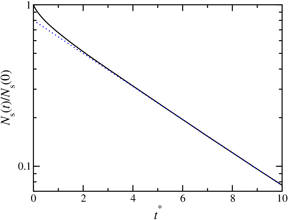
In each analyzed configuration we select a number of surface molecules, (typically is our optimal choice here) which self-consistently define the IS. The averages of the surface self-diffusion properties require us to follow the individual history of each of these molecules, i.e. to identify their permanence, exit, and possible reentrance in the IS list. All the reported surface diffusion properties are associated to the movement of molecules that stay continuously in the list of IS molecules, and this requirement sets a clear limitation on the avaliable sampling times. In Figure 1, represents the mean number of molecules which remain at the IS for, at least, a time ; the exponential decay , with a typical decay time, or residence time of (at ), which we also list in Table 1. This treatment mirrors the classical definition of the bulk residence time as the exponential decay time for the process by which neighboring molecules drift apart.Impey et al. 1983 It is also useful to keep in mind that for the case of Argon with the usual LJ parameters and nm one unit of reduced time corresponds to picoseconds. Thus, the decay time would be approximately ps for Argon.
This short value for the residence time implies that the sampling size would rapidly decrease (and the statistical noise increase) for large . The extrapolation to of this exponential decay at longer times indicates that about of the molecules at the IS will leave it at the constant rate of , associated to the long time exponential decay, while the remaining of the molecules get out of the IS much faster, sometimes to undergo a rapid reentrance. These molecules may be regarded as those which are only marginally associated to the outmost liquid layer, e.g. those which may be interpreted either as a local intrusion of the IS towards the bulk liquid, or alternatively as a local extrusion of the next-outmost layer towards the surface. The disordered structure of the liquid makes the existence of such ambiguities unavoidable, and different recipes to identify the IS from the molecular positions could make different assignments to those molecules to be in, or out of, the list of surface molecules. That is what makes the concept of the outmost liquid layer a soft one, but at the same time a rather robust one, since any reasonable choice of the tunable parameters would agree in the selection of the large majority of the surface molecules. For the diffusion properties analyzed here there is a further advantage, since the relevant information to get the effective surface diffusion coefficients comes from the sampling of molecular displacements at the longest possible times, which automatically selects the properties of those molecules with long permanence at the surface, representing the outmost liquid layer with any sensible choice for the parameters in the IS definition. The only practical inconvenience of the rapid turnover of some surface molecules is that the time interval between analyzed configurations, , has to be short enough to make sure that the estimation of is not affected by further reduction — in practice that is achieved, at , with , when only about two and a half surface molecules are changed on average between consecutive configurations.Chacón et al.

The mean profile of the whole system, , and that restricted to the surface molecules, , are presented in Figure 2, the later having a typical Gaussian shape which represents the fluctuations of the IS, and which becomes wider with increasing temperature and transverse sizes of the simulation box. Notice that despite the mean profile character of , all the selected surface molecules lie exactly on the instantaneous IS, we may therefore use them to follow exactly the self-diffusion of the molecules at the outmost liquid layer, without the coarsening effect of the CW fluctuations if we were selecting the molecules within a fixed surface slab. Moreover, we may keep track of the mean profiles for surface molecules which have continuous permanence in the IS list for more than a time , thus defining a distribution , whose integral over is directly linked to the number of surface molecules older than ,
| (3) |
We may expect that any diffusion property sampled for relatively large times would correspond to molecules distributed as
| (4) |
where the time dependences factorizes into the same exponential decay as , and we define a -distribution of old surface molecules, , which is normalized to unity. The prefactor has been discussed above to be , i.e. representing about of the surface molecules. This is indeed the case, and in Figure 2 we compare the mean profile of the whole set of surface molecules, , and the distribution of old surface molecules normalized to , i.e., . The distribution of old surface molecules is narrower, and asymmetric with respect to the whole one, and that may be interpreted in terms of the rate at with molecules are incorporated to, or deleted from, the list of surface molecules, as a function of their position .
Since we select a fixed number of surface molecules in each configuration, the loss of molecules from the IS layer, either towards the liquid or the vapor sides, is always compensated by the incorporation of new ones, and the time reversal symmetry of the MD guarantees that the inflow and outflow of surface molecules at a given value of are identical. We denote by that input/output rate per molecule, which may be directly sampled along our simulations and are presented in Figure 3, together with , for ease of comparison. The results are fairly well compatible with rates being independent of the previous permanence time of the molecule at the IS, so that
| (5) |
which for large implies
| (6) |

The shape of is clearly composed of two contributions: a large peak corresponding to the exit/entrance of surface molecules to/from the bulk liquid, an a much smaller one corresponding to the exit/entrance of surface molecules to/from the bulk vapor. In the following section we show how to extract the surface diffusion coefficients from the information from the observed displacements of the surface molecules, and the information on their turnover distributions contained in and .
III Diffusion in the bulk, and at the intrinsic surface
We discuss diffusion for the particular choice of temperature , in three different cases: bulk diffusion, diffusion parallel to the interface, and diffusion perpendicular to it.
III.1 Diffusion in the bulk
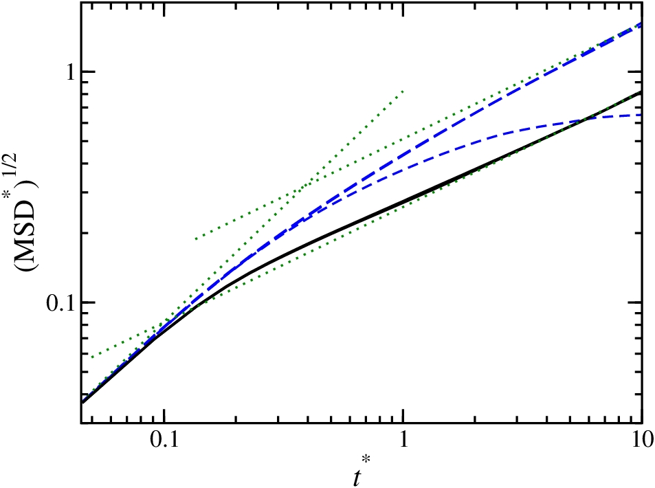
In Figure 4 we plot the square root of the MSD for the , , and components of the displacement versus time for the bulk liquid phase. At short times all curves tend to the same line, with a slope of . This is the ballistic regime: times so short that collisions can be neglected. In this case the Maxwellian distribution for velocities directly provides a value for the MSD
| (7) |
which is the dotted line in the graph.
At longer times a diffusive regime is reached, with the Einstein relation for each of the three Cartesian coordinates because of isotropy:
| (8) |
We indeed find no difference between the three components of the bulk. From linear interpolation of this line in the - graph one reads , in good agreement with previous data,Meier et al. 2004; Liu et al. 2004 see Table 1.
The time for the crossover between the ballistic and the diffusive regimes can be estimated from the crossing of the two linear regression lines. In this case this is . The corresponding mean displacement in each direction would be if read from the intercept of the lines, or from the MSD curves at . We also list these numbers in Table 2, where we will also include results for other temperatures that will be discussed in the next Section. Since the density is , assuming a local coordination close to the FCC packing, the typical intermolecular distance would be , and collisions would take place with typical displacements around , where is the minimum of the LJ potential, . This prediction yields , consistent with the values found.
| model | source | ||||||
|---|---|---|---|---|---|---|---|
| SA | this work | ||||||
| this work | |||||||
| LJ | Liu et al.Liu et al. 2004 | ||||||
| Meier et al.Meier et al. 2004 | |||||||
| LJ | this work | ||||||
| Meier et al.Meier et al. 2004 |
III.2 Diffusion parallel to the interface
Turning to the molecules at the interface, i.e. those selected as surface molecules by the intrinsic sampling method, their MDS, along the three Cartesian coordinates also plotted in Figure 4. The ballistic regime at short times is the same for all three components, and the same as for the bulk; but at longer times the curves are very different from the bulk, the and , parallel, components remaining indistinguishable, the component differing. We focus on the parallel diffusion in this section, for which we could expect the first two relations of Eq. (8) to hold, but with a different value of the diffusion coefficient:
| (9) |
At long times, the MSD for the parallel components of our surface molecules show this expected linear growth with limit, and we find , Therefore, the parallel diffusion coefficient is almost four times larger than the bulk one. This remarkable difference, with similar factors, had already been reported in works on water,Townsend and Rice 1991; Taylor et al. 1996; Liu et al. 2004 ethanol,Taylor and Shields 2003 dimethyl sulfoxide,Senapati 2002 and liquid-liquid interfaces in LJ mixturesMeyer et al. 1988; Buhn et al. 2004 (although not all of these works discriminate different components of the diffusion coefficient) — we should remark that, on the other hand, very little change has been obtained for liquid-liquid interfaces in mixtures of water and other polar liquids.Benjamin 1992; Michael and Benjamin 1998 Two works consider the liquid-vapor interface of the LJ fluid: a value of , at a similar temperature of , is reported in Ref. Liu et al. 2004 (also included in Table 1 ), in good agreement with our result. On the other hand, Ref. González and González 2006 find only a twofold increase over the bulk diffusion coefficient, even if their choice of temperature is again very close, .
The time for the crossover between the ballistic and the diffusive regimes is . The corresponding mean displacement in each is either (from the intercept of the lines), or (from the MSD curves). This means that the same approximate increase with respect to the bulk by a factor of about three applies to the characteristic time between collisions, the characteristic length between collisions, and the diffusion coefficient (this is of course consistent with ).
As shown in Figure 4, the crossover from the ballistic to the diffusive behavior is quite different for the bulk and the surface molecules. The MSD in the bulk converges to the diffusive regime from above, i.e. after leaving the rapid ballistic regime, there is a time interval in which the relative growth of the MSD is slower than in the asymptotic diffusive regime. On the contrary, the parallel diffusion of the surface molecules shows a much smoother interpolation between the two limiting regimes, which may be interpreted as a signature of the stronger disorder in the correlation structure at the surface, causing a wider time distribution for molecular rearrangement leading to the diffusive regime. The MSD is always below the asymptotic diffusion, and with very little difference between the normal (), and transverse () directions up to , and displacements , which are approximately half way between the ballistic prediction and the observed results for bulk for the same . These values are also listed in Table 2, under the heading of “split.”
The surface molecules reach the diffusive regime only for typical displacements larger than one molecular diameter , which require a time similar to the residence time. If we compute the time needed to diffuse to a displacement of we find , a value very close to that of ( in reduced units). This means that only about one third of the molecules at the surface () remain in it before diffusing a transverse distance similar to their diameter. We have to bear in mind the exponential decay for the number of molecules which remain at the surface after a time — e.g. a molecule would likely move a distance on the surface in a time , while in the bulk it would need typical times times larger to diffuse the same distance. However, less than two percent of the surface molecules () would remain as such for and longer times, so that the large value of has limited relevance for the actual surface kinetics. The turnover process of molecules from the surface to the bulk phases, and its reverse, would be at least as relevant as the diffusion on the surface. Therefore, it is most important to analyze that turnover process, beyond its simple description in terms of the typical time . In the next subsection we show how the intrinsic sampling method may also give an effective diffusion coefficient for the movement of the surface molecules in the direction, in their wandering which will eventually take them out of the surface.
III.3 Diffusion perpendicular to the surface
The naive relation
| (10) |
is bound to fail if we restrict the averaging to the molecules at the surface — these are limited in space to the region about which the IS fluctuates (both in position and in time). The MSD for the coordinate will therefore tend to a constant value equal to the squared width of the surface molecules density profile. An intermediate diffusive regime between ballistic behavior and this final plateau may appear sometimes, but there is no reason to expect this in general. Indeed, this is not the case in the situation considered here, as is obvious from the dashed line in Figure 4.
We show how to go beyond this naive prediction in a series of steps. First, Einstein’s equation is more general than Eq. (10): this would be the second moment of a probability distribution:
| (11) |
This, of course, is the solution to the diffusion equation
| (12) |
with an initial Dirac delta function distribution: , and vanishing values of and its flux for large . In our MD simulations that would correspond to selecting molecules which at the time were within a very thin slab in the direction, and which in terms of their displacement , would diffuse to have a probability distribution after a time .
The same experiment could be done selecting the molecules on the intrinsic surface at time , and following their displacement with , but that would soon mix the surface and bulk diffusion as commented in the introduction. Alternatively, we may represent in only the position of those molecules which have been continuously at the IS from . That probability distribution would not expand indefinitely, as required by the constant value of the MSD for the component at long times in Figure 4. That effect can be ascribed to an external potential that constrains surface molecules to a particular location in space. Indeed, this potential should be identified with a potential of mean force (PMF): the mean-field description of the action of all other molecules on the one diffusing on the surface. Our diffusion equation would now be a Smoluchowski equation:
| (13) |
(application of Smoluchowski equations to diffusion in non homogeneous media can also be found in Refs. van Hijkoop et al. 2007; Liu et al. 2004). The solution to this equation in the steady state would be an equilibrium distribution
| (14) |
A final ingredient comes from the fact that molecules are continously leaving the IS, a fact which may be incorporated through a loss term in the Smoluchowski equation:
| (15) |
where we have to plug the input/output frequency at each position, , discussed above and shown in Figure 3. The function solving this equation would not keep its normalization, since its integral will decay with time, as the probability that an initially selected surface molecule would remain at the surface at time .
For very long times we expect that, independently of the way we initially select them, the remaining surface molecules will factorize as in Equation (4): , in terms of the probability distribution for the coordinates of old surface molecules, in Figure 2, and decaying with the typical time , so that (15) becomes
| (16) |
which, for a given could be used to get the effective potential of mean force which is compatible with forms of and obtained from our MD simulations, and related to the turnover time through (6). The potential of mean force could be easily obtained by integration of Equation (16):
| (17) |
Thus, the only unknown in Equation (15) is the parameter , which is required both to get and to set the scale in the time variation of . If we integrate that equation from the equilibrium probability distribution for all the surface molecules, it would evolve in time towards the exponentially decaying distribution of old surface molecules, and we could get through the comparison of the actual evolution of with the solution of the generalized Smoluchowski equation. A better estimation of may be obtained if we start with a narrower probability distribution , representing the surface molecules which are initially within a thin slab around a given . The evolution of this probability distribution shows a first stage of broadening, dominated by the diffusion so that . In the later stage, the confining effects of , and the losses regulated by will saturate the MDS and lead to the mature distribution , with a prefactor which would depend on the value of . The description of both the early and late stages with the same effective diffusion coefficient, which should also be fairly independent of the initial position of the chosen surface molecules, is a strong requirement to confirm the validity of the whole scheme, and hence the relevance of the best fitting value of as a true normal surface diffusion coefficient.
In Figure 5 we show results for the time evolution of a peak initially at from the maximum of (its negative sign meaning toward the vapor side), with an initial width of . The whole evolution of the can be traced, but we will just focus on its main features: its mean position, its MSD, and its decay (normalization). We try to fit these three curves with the numerical solution of Eq. (15), and we obtain a very good agreement fitting a perpendicular diffusion coefficient that is comparable to, but smaller than the parallel one. Of course, the exponential decay of reproduces the previous value of (see dotted line in Fig. 5). We have checked that our results are largely independent of the initial position , except for peaks very close to the liquid phase. Indeed, the procedure seems to fail somewhat on this side, presumably due to the more involved nature of the process close to the liquid, with “interstitial” molecules, fluctuating rapidly (ballistically) from being considered as belonging or not to the IS. Those are again the expected limitations of any attempt to locate the outmost liquid layer, and we should be ready to accept some degree of “softness” in that concept. Nevertheless, the whole procedure provides a fairly well defined value of the normal surface diffusion, with a value between those of the bulk and the tangential surface diffusion, and close to the later.
Remarkably, there is only one work, to our knowledge, that discusses normal diffusion in a liquid-vapor interface, Ref. Liu et al. 2004. They report a value (also included in Table 1 ) that is lower than ours, and closer to the bulk value. This is presumably due to their use of slabs, by which some of slower bulk diffusion is mixed with the normal diffusion. The remaining works all discuss liquid-liquid interfaces, providing very similar values for both diffusion coefficients at the interface,Meyer et al. 1988; Buhn et al. 2004 or lower values for the normal coefficientBenjamin 1992; Michael and Benjamin 1998 (even lower, in fact, than the bulk values). It is our feeling that this discrepancy stems mainly from the saturation of the curve corresponding to normal diffusion that has been discussed (short dashed curve in Figure 4): if a diffusion is computed for times shorter than the split time, a similar value for both coefficients will be found; but for longer times, an (effective) lower normal coefficient will be obtained.

| bulk | IS | split | |||||||||
|---|---|---|---|---|---|---|---|---|---|---|---|
| model | |||||||||||
| SA | |||||||||||
| LJ | |||||||||||
| LJ | |||||||||||
IV Discussion
In order to support our main claims, we have performed simulations at other temperatures. We would like to consider temperatures higher and lower than the one considered. Hence, we have collected results for the LJ liquid-vapor interface at a temperature higher, . It is not possible in principle to lower the temperature below the triple point of LJ — hence, in order to observe the influence of a sizable drop in temperature, we have considered the soft alkali (SA) potential of Ref. Chacón and Tarazona 2003. The parameters in this model have a similar meaning to the ones in the LJ: is the distance at which the potential vanishes and is related to the volume integral of the intermolecular potential function. Thus, the estimated critical temperature for this model is , similar to the one of the LJ fluid (). This is a potential engineered to result in a very low triple point temperature of . We have considered a temperature of . The lateral size is , and the number of components employed in the IS Fourier analysis is . In addition, the optimum value of the surface density is, for this model . The curves showing the square root of the MSD as a function of time, for the two temperatures, are given in Figure 6.
The results for the residence time and for the diffusion coefficients are included in Table 1. We see that with increasing temperature decay diffusion becomes faster and residence times shorter, as is to be expected. The ratio is about for the higher temperature (LJ fluid), since the increase in is less drastic than that in . For the lower temperature (SA fluid) this ratio is about : in this case the reduction in turns out to be more drastic than that in . This is probably due to the fluid phase being already very dense, while the molecules at the surface still have the option of hopping along it — surface diffusion is therefore reduced due to the prevalence of energetic attraction (exerted mainly from the bulk liquid) over entropy at lower temperatures.

We have also repeated the analysis of typical times and lengths for the curves in Figure 6, and collected this information in Table 2. The most obvious correlation is between the time needed to diffuse a length of , and the residence time. In all three cases, these two quantities are nearly equal. This corresponds to a natural assumption of a certain isotropy in the diffusion process: by the time a molecule at the IS has displaced a length of one molecular diameter, it is likely that the molecule has also left the IS (which is of course consistent with the IS being of molecular width). In other words, the product of and should be nearly constant, which indeed is true, providing a typical length of in all three cases.
There seems to be some agreement in the split length, the approximate displacement beyond which the parallel and perpendicular diffusion curves split, with a value around in all cases. Other correlations are seen to be model-dependent. For example, the trend for typical bulk crossover times and lengths differs in the SA model due to its shallower potential well. Indeed, the argument given above in terms of a local coordination close to the FCC packing is still valid for the higher temperature, yielding a value of (to compare against ), but fails for the SA model, with a value of that is below the appropriate .
In addition to varying the temperature, it is natural to explore the dependence of diffusion with the interfacial area. On one hand, the CW framework leads us to think that there could be a change of with the area. On the other hand, if this quantity is a true intrinsic property of the surface, it should be area-independent. In order to explore this possibility, we have scaled the lateral length of our simulation box, , by factors of , , , and (i.e., the area going from to times the original). For the last two cases, we have increased the number of molecules to and , respectively (otherwise, the liquid film would have been too thin); we have also enlarged the cell in the direction, with for the smallest area in order to accommodate a thicker liquid slab. In order to keep the same resolution in the IS Fourier treatment, the functions for the original area will now be , , , and , respectively.
As shown in Figure 7, functions and contract for smaller areas and stretch for larger ones, as is to be expected from the general broadening due to CWs. (In order to obtain these curves, it is important that the various properties of the IS should be computed by subtracting the value of the (constant) mode — otherwise, bulk density fluctuations produce a spurious broadening of the distributions at smaller areas,Chacón and Tarazona 2003 contrary to the contraction that is found). Nevertheless, the repetition of the analysis by means of the Smoluchowski Equation (15), shows no measurable dependence of with the area within our error bar. This supports the identification of as a true intrinsic property of the surface, and confirms the methods described. Indeed, simpler methods based on dividing the system in slabs,Buhn et al. 2004; Liu et al. 2004 or selected “outmost” moleculesTaylor et al. 1996; Taylor and Shields 2003 would have resulted in a clear dependence of with the area.

V Conclusions and future work
We have described an application of the intrinsic sampling method to the analysis of dynamical processes at the liquid-vapor interface. The main conclusion is that a liquid surface is a region of enhanced molecular mobility, with respect to that in the bulk liquid, but without strong anisotropy. The characterization of the normal diffusion constant for the molecules at the outmost liquid layer requires a much more elaborated method that for the transverse component, but at the end of the day we get similar values for and , both at high and low temperatures for the simple liquid models studies in this article. This fact is consistent with our results for the residence time, which governs turnover rate, i.e., the rate at which molecules enter and leave the intrinsic surface — a time that turns out to be comparable to the typical times for the threshold of diffusion. Thus, the typical time required for a molecule to travel a distance on the order of a molecular diameter is very similar to its residence time as a surface molecule. Therefore, even if diffusion coefficients can still be computed for molecules that stay at the surface for times long enough, the turnover processes are equally important when discussing the dynamical properties of the interface. We have discussed two main features of these processes: the overall residence time, and the input/output rate per molecule, , the spacial distribution function of the turnover rate.
The particular details of interfacial dynamics will be, of course, model-dependent. We next provide some relevant cases on which the method describe here could be applied. References will be given to previous works on these systems, but we would like to emphasize that these works have employed the usual approach (by means of slabs), therefore the present approach (by means of the IS) could shed new light on the structure and dynamics of systems of considerable applied interest.
The most important applications of this technique would now be realistic models of complex fluids, such as the liquid-vapor interface of waterLiu et al. 2005; Liu et al. 2004 In this case, the more orderly nature of liquid phase, and the high surface tension, are likely to provide additional stability for the molecules at the interface, thereby leading to longer residence times and more surface molecules reaching the diffusion regime. We have already started an effort to study this system from the point of view presented in this article — in particular, the discrepancy in our value of the normal diffusion coefficient for the LJ fluid with results of Ref. Liu et al. 2004 suggest that the corresponding values for water will likewise differ. We also intend to employ this approach to clarify the controversy surrounding normal diffusion in liquid-liquid interfaces.Meyer et al. 1988; Benjamin 1992; Michael and Benjamin 1998; Buhn et al. 2004
Similar systems of interest include aqueous solutionsPaul and Chandra 2005a; Paul and Chandra 2005b; Paul and Chandra 2005c; Chang and Dang 2006 (the later is a useful review on ion solvation at liquid surfaces) and surfactants at interfaces.Chanda et al. 2005; Chanda and Bandyopadhyay 2005; Chanda and Bandyopadhyay 2006; Clavero et al. 2007 Surfactants will be usually located at the surface, and most will reach the diffusive regime. The relationship between structure and dynamics is specially interesting in systems with strong profiling, such as liquid metals,González and González 2006 confined water,Martins et al. 2004; Sega et al. 2005; Marti et al. 2006; van Hijkoop et al. 2007; Lee and Rossky 1994 and liquid-solid interfaces.Thomas and McGaughey 2007 Similarly, diffusion in amphiphilic bilayer structures, Bhide and Berkowitz 2005; Sega et al. 2005 micelles,Pal et al. 2005 and microemulsions can be described in a manner similar to the one presented here.
VI Acknowledgments
Financial support for this work has been provided by the Dirección General de Investigación, Ministerio de Ciencia y Tecnología of Spain, under grants FIS2004-05035-C03, FIS2007-65869-C03, and CTQ2005-00296/PPQ and Comunidad Autónoma de Madrid under program MOSSNOHO-CM (S-0505/Esp-0299).
References
- Buff et al. (1965) F. P. Buff, R. A. Lovett, and F. H. Stillinger, Phys. Rev. Lett. 15, 621 (1965).
- Evans (1979) R. Evans, Adv. Phys. 28, 143 (1979).
- Rowlinson and Widom (2002) J. Rowlinson and B. Widom, Molecular Theory of Capillarity (Dover, 2002).
- Toxvaerd and Stecki (1995) S. Toxvaerd and J. Stecki, J. Chem. Phys. 102, 7163 (1995).
- Sides et al. (1999) S. W. Sides, G. S. Grest, and M.-D. Lacasse, Phys. Rev. E 60, 6708 (1999).
- Townsend and Rice (1991) R. M. Townsend and S. A. Rice, J. Chem. Phys. 94, 2207 (1991).
- Senapati (2002) S. Senapati, J. Chem. Phys. 117, 1812 (2002).
- Meyer et al. (1988) M. Meyer, M. Mareschal, and M. Hayoun, J. Chem. Phys. 89, 1067 (1988).
- Benjamin (1992) I. Benjamin, J. Chem. Phys. 97, 1432 (1992).
- Michael and Benjamin (1998) D. Michael and I. Benjamin, J. Electroanal. Chem. 450, 335 (1998).
- Buhn et al. (2004) J. B. Buhn, P. A. Bopp, and M. J. Hampe, Fluid Phase Equil. 224, 221 (2004).
- Liu et al. (2004) P. Liu, E. Harder, and B. Berne, J. Phys. Chem. B 108, 6595 (2004).
- Chanda et al. (2005) J. Chanda, S. Chakraborty, and S. Bandyopadhyay, J. Phys. Chem. B 109, 471 (2005).
- Chanda and Bandyopadhyay (2005) J. Chanda and S. Bandyopadhyay, J. Chem. Theory Comput. 1, 963 (2005).
- Chanda and Bandyopadhyay (2006) J. Chanda and S. Bandyopadhyay, J. Phys. Chem. B 110, 23482 (2006).
- Paul and Chandra (2005a) S. Paul and A. Chandra, J. Chem. Phys. 123, 184706 (2005a).
- Paul and Chandra (2005b) S. Paul and A. Chandra, J. Chem. Phys. 123, 174712 (2005b).
- Paul and Chandra (2005c) S. Paul and A. Chandra, J. Chem. Theory Comput. 1, 1221 (2005c).
- Liu et al. (2005) P. Liu, E. Harder, and B. Berne, J. Phys. Chem. B 109, 2949 (2005).
- González and González (2006) L. E. González and D. J. González, J. Phys.: Cond. Matt. 18, 11021 (2006).
- Clavero et al. (2007) E. Clavero, J. Rodriguez, and D. Laria, J. Chem. Phys. 127, 124704 (2007).
- Lee and Rossky (1994) S. H. Lee and P. J. Rossky, J. Chem. Phys. 100, 3334 (1994).
- Martins et al. (2004) L. Martins, M. Skaf, and B. Ladanyi, J. Phys. Chem. B 108, 19687 (2004).
- Bhide and Berkowitz (2005) S. Y. Bhide and M. L. Berkowitz, J. Chem. Phys. 123, 224702 (2005).
- Sega et al. (2005) M. Sega, R. Vallauri, and S. Melchionna, Phys. Rev. E 72, 041201 (2005).
- Pal et al. (2005) S. Pal, B. Bagchi, and S. Balasubramanian, J. Phys. Chem. B 109, 12879 (2005).
- Marti et al. (2006) J. Marti, G. Nagy, E. Guardia, and M. Gordillo, J. Phys. Chem. B 110, 23987 (2006).
- van Hijkoop et al. (2007) V. J. van Hijkoop, A. J. Dammers, K. Malek, and M.-O. Coppens, J. Chem. Phys. 127, 085101 (2007).
- Thomas and McGaughey (2007) J. A. Thomas and A. J. H. McGaughey, J. Chem. Phys. 126, 034707 (2007).
- Taylor et al. (1996) R. Taylor, L. Dang, and B. Garrett, J. Phys. Chem. 100, 11720 (1996).
- Taylor and Shields (2003) R. S. Taylor and R. L. Shields, J. Chem. Phys. 119, 12569 (2003).
- Pershan (2000) P. S. Pershan, Colloids and Surf. A 171, 149 (2000).
- Chacón et al. (2001) E. Chacón, M. Reinaldo-Falagán, E. Velasco, and P. Tarazona, Phys. Rev. Lett. 87, 166101 (2001).
- Velasco et al. (2002) E. Velasco, P. Tarazona, M. Reinaldo-Falagan, and E. Chacon, J. Chem. Phys. 117, 10777 (2002).
- Chacón and Tarazona (2003) E. Chacón and P. Tarazona, Phys. Rev. Lett. 91, 166103 (2003).
- Tarazona and Chacon (2004) P. Tarazona and E. Chacon, Phys. Rev. E 70, 235407 (2004).
- Chacón and Tarazona (2005) E. Chacón and P. Tarazona, J. Phys.: Cond. Matter 17, S3493 (2005).
- Chacon et al. (2006a) E. Chacon, P. Tarazona, and L. E. Gonzalez, Phys. Rev. E 74, 224201 (2006a).
- Chacon et al. (2006b) E. Chacon, P. Tarazona, and J. Alejandre, J. Chem. Phys. 125, 014709 (2006b).
- (40) E. Chacón, D. Duque, and P. Tarazona, to be published.
- Smith (2006) W. Smith, Mol. Sim. 32, 933 (2006).
- Mastny and de Pablo (2007) E. A. Mastny and J. J. de Pablo, J. Chem. Phys. 127, 104504 (2007).
- Frenkel and Smit (2002) D. Frenkel and B. Smit, Understanding Molecular Simulation (Academic Press, 2002), 2nd ed.
- Impey et al. (1983) R. W. Impey, P. A. Madden, and I. R. McDonald, J. Phys. Chem. 87, 5071 (1983).
- Meier et al. (2004) K. Meier, A. Laesecke, and S. Kabelac, J. Chem. Phys. 121, 9526 (2004).
- Chang and Dang (2006) T.-M. Chang and L. Dang, Chem. Rev. 106, 1305 (2006).