Radiatively Induced Spontaneous Symmetry Breaking by Wilson Line in a Warped Extra Dimension
Abstract
We investigate the dynamical gauge-Higgs unification in the Randall-Sundrum (RS) space-time. We study the dynamical gauge-Higgs unification in the gauge theory with a bulk fermion in the RS space-time. We evaluate the contribution from fermion loop to the one-loop effective potential with respect to the Wilson-line phase, and study the dynamical gauge symmetry breaking. We also apply this mechanism of the gauge symmetry breaking to the electroweak gauge-Higgs unification in the RS space-time. Especially we numerically studied a gauge model as a toy model of electroweak gauge-Higgs unification in the RS space-time. We introduce an adjoint fermion into the model to break the gauge symmetry and to obtain the electromagnetic symmetry. We found that in this model the ratio of -boson mass to -boson varies with respect to the Wilson-line phase even at the tree level. We also propose a dynamical mechanism of tuning the ratio to the experimental value by introducing bulk scalars or bulk fermions with twisted boundary conditions. In these models the Higgs can vary in mass between zero and .
I Introduction
The standard model has been in good agreement with current experimental data. The origin of the electroweak symmetry breaking, however, has not yet confirmed. As an alternative to the Higgs mechanism, the electroweak gauge-Higgs unification (EWGHU) has been considered for many years (for early works, see Fairlie; Manton; Krasnikov). In the EWGHU, the Higgs field is regarded as an extra-dimensional component of the gauge field in higher-dimensional space-time. If the gauge group is non-Abelian and the spatial extra dimension is multiply-connected, then the gauge symmetry can be broken by the non-Abelian Wilson line phase in the extra dimension (i.e., broken through the Hosotani mechanism) Hosotanimechanism; Witten85. Furthermore, such Wilson line phases can be dynamically induced Hosotanimechanism; Hosotani89; Hosotani02. One can define the effective potential with respect to the Wilson-line phases. The Wilson-line phases are dynamically selected as the phases that minimize the effective potential. This dynamical mechanism of the gauge-symmetry breaking by Wilson-line phases is referred as the dynamical gauge-Higgs unification. In the dynamical gauge-Higgs unification, both of the size of the mass and the magnitudes of the effective potential are almost of the order of size of the extra dimensions. Therefore, since possibilities of the TeV-scale extra dimensions are pointed out Antoniadis90; LED, the EWGHU scenario has been extensively studied in the context of the dynamical gauge-Higgs unification HIL; Nomura; Antoniadis_Benakli; Choi; Panico; Antoniadis-Benakli-Quiros; Lim-Kubo-Yamashita; Hosotani04; bulkmass; Murayama; Wudka06; finiteness; Haba-Takenaga-Yamashita; Sakamoto06; Cacciapaglia; GHU-Yukawa; EWGHU_others; adjoint-fermion.
However, in the construction of a realistic model of the EWGHU in the flat extra dimension, we encounter several obstacles. To see this, let us consider the models with “flat extra dimensions”. Here models with flat extra dimensions are models such that (i) Extra dimensional space has vanishing curvature (e.g., a circle or -torus ). (ii) The metric of the spacetime is assumed to be “factorizable”, in other words, the metric of the four-dimensional space-time can be independent of coordinates of extra dimensions. The obstacles we will see in these models are as follows.
- (a)
In models of the EWGHU with dynamical gauge-Higgs unification in a flat extra dimension, we obtain too small Higgs mass. In Hosotani04 the Higgs mass is estimated to be , where with the four-dimensional (4D) weak coupling . With and , we obtain , which contradicts the observation.11 1 Ways of pushing up the Higgs mass by fine-tuning of the Wilson-line phase are studied in Haba-Takenaga-Yamashita.
- (b)
In models of the EWGHU in the flat extra dimension, the mass of the quarks and leptons tend to be universal and the mixing matrix of quarks to be diagonal, because the gauge coupling constant yields the ‘‘Yukawa couplings’’ of fermions to the Higgs in the gauge-Higgs unification. Therefore, it needs some other mechanisms to induce large mass hierarchy and mixings among fermions.22 2 Some ways to obtain the Yukawa hierarchy in the gauge-Higgs unification are discussed in Murayama; GHU-Yukawa.
- (c)
In the models in the flat extra dimension, one of the simplest way to give different masses to fermions is to assign the different bulk mass term to each fermion. Then, in the EWGHU the mass of the lowest Kaluza-Klein (KK) mode of such a bulk fermion is estimated to be , with the Wilson line phase , compactification radius and bulk mass of the fermion . Thus, a fermion with larger (smaller) bulk mass can be heavier (lighter) in the four dimensional effective theory. Since the effective potential decrease in size with increasing the bulk mass of the fermion HIL, it lead us to an odd conclusion: a light fermion (e.g., up-,down-quark or electron) has large contribution to the effective potential of the Higgs. The low energy dynamics of the EWGHU in the flat extra dimension looks very different from 4D models of the electroweak symmetry breaking by the Coleman-Weinberg (CW) mechanism CW.
In recent years, models of electroweak gauge-Higgs unification in the Randall-Sundrum (RS) space-time RS have been extensively studied Toms; Oda; Medina; Hosotani05; Hosotani06; Sakamura06; Contino03; AdS-deconstruct. We first summarize the merits of the dynamical gauge-Higgs unification in the RS space-time. They are
- (A)
The hierarchy between electroweak and a larger scale (e.g., the Planck scale) are explained by the nature of the RS space-time RS33 3 Attempts to obtain the large hierarchy within the framework of the flat extra dimension are seen in Haba-Takenaga-Yamashita; Sakamoto06., whereas the quadratic divergence of the Higgs mass is absent due to the higher-dimensional gauge symmetry Hosotanimechanism; HIL; finiteness.
- (B)
The extra dimension of the RS has the orbifold topology . On such space-time, we can naturally obtain the chiral structure of fermions by boundary conditions at the fixed points. projection also yields the Higgs field in the fundamental representation of from the gauge field in the adjoint representation of a gauge group which includes the .
- (C)
In the RS space-time, we can obtain large mass differences among fermions by tuning bulk mass parameters of fermions of order of unity Neubert. In the same way we can obtain large mass hierarchy among fermions in the EWGHU in the RS space-time Hosotani06.
- (D)
The mass of the Higgs will be lifted up to a few hundred GeV when we consider the dynamical gauge-Higgs unification in the RS space-time Hosotani05.
- (E)
When we implement the standard model in the RS space-time, the Higgs field (i.e., the 5th-dimensional component of the gauge field) is naturally localized on the TeV brane. We note that such a localization of the Higgs on the TeV brane is usually required in the context of the 5D extension of the standard model in the RS space-time GP; RSbulk; Higgs-Localization.
The dynamical gauge-Higgs unification in the Randall-Sundrum space-time is first considered in Toms and effective potential by fermion without bulk mass is evaluated in it. An appropriate form of the background gauge in the RS space-time and the calculation of the effective potential from gauge-ghost loop is studied in Oda. The phenomenological studies of the EWGHU in the RS space-time are seen in Hosotani05; Hosotani06; Sakamura06; Medina. We note that there are series of works Contino03, based on the AdS/CFT dual or “holographic” picture AdSCFT. The Wilson-line dynamics in the warped extra dimension has also been studied in AdS-deconstruct by means of the dimensional deconstruction deconstruction.
In the present paper we investigate the dynamical gauge-Higgs unification in the Randall-Sundrum space-time. The aim of the present paper is the following threefold. First, we evaluate the effective potential of Wilson line and discuss the gauge symmetry breaking by the dynamical gauge-Higgs unification and to evaluate the mass of the Higgs field. Especially we are interested in the one-loop effective potential for the loop of fermion with a bulk mass term. Second, we make clear the relation between the fermion mass spectrum and the effective potential in this model. In the case of warped extra dimension, the lowest KK mass of the fermion decreases in size with increasing absolute value of the bulk mass. Therefore we expect that in the RS space-time, a heavy fermion in the 4D effective theory will have large contribution to the effective potential and a light one has small contribution, as we have seen in the CW mechanism. We will demonstrate it is true. Third, we use the dynamical gauge-Higgs unification in the RS space-time to construct a model of the EWGHU with realistic mass spectrum of fermions and a Higgs potential.
The present paper is organized as follows. In Section II, we study the gauge model in the RS space-time and evaluate the one-loop effective potentials from the fermion loop and see how the effective potential and the gauge symmetry depends on the bulk muss term of the fermion. In Section III, as an application of the dynamical gauge-Higgs unification in the RS space-time, we reconsider the gauge model as a toy model of EWGHU in the warped extra dimension. Section IV is devoted to the summary and comments. In Appendix A Approximation formulas of low-energy mass spectrum of fermions are collected.
II Dynamical Gauge-Higgs Unification in the RS Space-Time
We consider the gauge theory in the the RS two-brane model RS. The RS space-time is a slice of five-dimensional anti-de Sitter space-time , and the metric of the RS space-time can be written as
| (1) |
where the five-dimensional coordinates are ( and ). is the 4-dimensional metric and . We assume that the function has the periodicity and the reflection symmetry at () with and , where is the compactification radius. In the present paper we assume that is already fixed by some mechanisms (e.g. Goldberger-Wise mechanism GW). For , we write , where is referred as the curvature of the . Two boundaries and are referred as “Planck brane” and “TeV brane”, respectively.
We consider a gauge theory in this space-time. We also include a Dirac fermion in the fundamental representation, or in the adjoint representation. The action of the gauge field and the fermion in the bulk space-time can be given by , where and , () are given by
| (2) | |||||
| (3) |
where is the field strength : and is the gauge field. and are the gauge-fixing and the Faddeev-Popov Lagrangian, respectively. The five dimensional -matrices are defined by (Small Latin indices represent Lorentz indices and ), and . is an inverse of the fünfbein. and are absolute values of determinants of the metric tensor and the fünfbein, respectively and is satisfied. and are dimensionless bulk mass parameters for and , respectively. is the sign function: for (). We decompose a field in the adjoint representation and in the fundamental representation into and ( is the Pauli matrices), respectively.
As a gauge fixing, we choose the background gauge. We separate the gauge field into background and quantum fluctuation : . In the background gauge we write covariant derivatives of the gauge field, fermions in the fundamental and adjoint representation as
| (4) | |||||
| (5) | |||||
| (6) |
where is the spin connection and (), and other components vanish. We expect only -component of the gauge field can have non-vanishing vacuum expectation value(VEV), i.e., . By choosing appropriate gauge fixing term Oda and corresponding ghost term in the action, we obtain the quadratic action of and the ghost field :
| (7) |
where () and , respectively. For later use, we introduce a new coordinate , which is defined by (). With this coordinate, equations of motion for gauge fields , () and fermionic fields are given by
| (8) | |||||
| (9) | |||||
| (10) |
where . Gauge fields and fundamental (adjoint) fermions () are decomposed into their Kaluza-Klein modes:
| (11) | |||||
| (12) |
Here the left-(right-)handed fermions are defined by . When vanishes, or when an adjoint field commute with the VEV of gauge field: , we can simplify Eqs. (8), (9), (10), and we obtain wave equations for KK-mode functions as
| (13) | |||||
| (14) | |||||
| (15) | |||||
| (16) |
For a field we obtain non-zero mode () solutions for (13), (14), (15), (16) into the form of
| (17) |
with , , and , for .
At the two boundaries (), we define the boundary conditions, namely, the odd boundary condition: and the even boundary condition: , when is the gauge boson or the ghost. For fermions , we should write boundary conditions as
| (18) |
where . For the KK mode functions , the odd boundary conditions can be written as
| (19) |
whereas even boundary conditions take the form of GP; Contino03:
| (20) |
where , and for , and , respectively. It would be convenient Hosotani06 to rescale the KK mode functions (17) and to define
| (21) |
where for , respectively.44 4 We choose for . With (21), we can rewrite even boundary conditions (20) into the form of .
In this model, the extra-dimensional components of the gauge field can develop a non-zero vacuum expectation value (VEV) . Furthermore, since the non-simply connected topology of the extra dimension of the RS space-time, we cannot gauge away the Wilson-line phase : . This phase can change the boundary condition and therefore can change mass spectrum of fields due to Aharonov-Bohm effect Aharonov-Bohm. To see this, in the following we will consider one of the simplest but non-trivial case. In the beginning, we turned off gauge VEV and impose a boundary condition on the theory. It is
| (22) |
here . This boundary conditions (22) arrows for and to have zero modes. Therefore this boundary condition break the gauge symmetry to with massless gauge boson . Due to the non-simply connected nature of topology of the extra dimension of the RS space-time, can develop a VEV. Without loss of generality, we can set in the direction of . As a zero-mode solution of (14), we set gauge VEV as
| (23) |
where is a constant parameter. The gauge symmetry can be broken, if and if the Wilson line phase does not commute with the generator of the : . In the following we refer the gauge which is represented by non-zero VEV (23) and boundary condition (22), as the “Aharonov-Bohm gauge” or the AB-gauge.
By using a gauge transformation
| (24) | |||||
| (25) |
we move to an another gauge . The boundary condition of the gauge fields are also changed to :
| (26) |
by the gauge transformation: . In Eq.(26), are given by
| (27) |
Thus we find that in this gauge the gauge field obey the twisted boundary condition (26) at , whereas the Wilson-line phase becomes trivial . We refer the gauge with vanishing gauge VEV and with the boundary condition (26) as the (twisted) boundary condition gauge or the BC-gauge.
In the analogous way, we can set boundary conditions and perform gauge transformations of fermions. We can write the boundary conditions of and in the AB-gauge as55 5 For simplicity, we assume that all boundary conditions take same form as gauge field, nevertheless the boundary conditions of all fermions are not necessarily the same as the gauge fields.
| (28) |
with . For simplicity, hereafter we set .
In the BC gauge, since the gauge VEV vanishes, we can solve the wave equations (13)(14)(15)(16) for , and . As an example, we consider the right-handed fundamental fermion with bulk mass . In the BC gauge, wave functions take the form of
| (29) |
where and are constant, and we set . By solving twisted boundary condition in BC gauge (or by going back to AB gauge by gauge transformation , with and considering the even (odd) boundary condition of () at ), we obtain conditions:
In the same way we can write the boundary condition of , and . These boundary condition can be written in the form of
| (34) |
where for , and for . The matrix is defined by
| (35) |
where for , , (), respectively. and are defined by
| (36) |
where for , and for . The factor depends on ’s representation of the gauge group. In case, when is in fundamental (adjoint) representation. The -th Kaluza-Klein state of the field has a mass , where the are defined as a -th smallest solution of the equation: . Defining
| (37) | |||||
(where ), we rewrite the condition as
| (38) |
where and are given by
Let be the -th smallest non-negative zeros of . Thus, the -th Kaluza-Klein mass of the field : is given by
| (46) |
In FIG. 1 we plot () which are first three smallest zeros of with .


We see that the mass spectrum largely depends on when is small, whereas the dependence on become smaller for larger (here we note that has a symmetry , as shown in Appendix B of Hosotani06).66 6 FIG. 1 of the present paper and FIG. 1 in Hosotani06 are similar to each other, although in each figure different parameters are changed ( in the former and in the latter.) From the dependence of as we have seen above, we can expect that the the effective potential, which is obtained by summing up all of the Kaluza-Klein mode, has large (small) dependence on when is small (large).
We evaluate the 1-loop effective potential in a similar way as CW. As an example we calculate the one-loop contribution of a fundamental fermion . This is given by
| (47) |
where defined as , is the renormalization scale, and is the -th positive-real solution of . The coefficient reflects the four degrees of freedom of a Dirac fermion and the minus sign for the fermion loop. After performing the dimensional regularization, we can write as
| (48) |
Here the summation can be rewritten as a contour integral:
| (49) |
where the path is a set of all circles surrounding each zeros of on the positive real axis. The contour integral in (49) can be calculated in a similar way to Toms; Oda; RSquantum. We find that -dependent part of is finite.
| (50) |
where is defined by
| (51) | |||||
with . This function has a symmetry , and a periodicity . The function (51) with becomes the same form as the integral in Eq. (18) of Oda. Furthermore, when we can rewrite as
| (52) | |||||
where is the polylogarithm and is the Riemann zeta function. can be expanded as , or expanded as . The expression (52) coincides with the result obtained in Sec. IV of Ref. Toms. The shapes of with respect to with different are similar with each other (FIG. 2).

We show dependence of amplitude on in FIG. 3.

In the case of flat extra dimension it is known HIL; bulkmass that the contribution to one-loop effective potential from a field dumps when the bulk mass of the field is much larger compared to (the inverse of) the size of the extra dimension. It is also true for the models in the RS space-time. However, in the RS space-time the relation between the effective potential and the 4-dimensional mass of the field is different from the case of flat extra dimension. Therefore a fermion with the large lowest KK mass can have a large contribution to the effective potential. To see this, let us see the relation between the magnitude of the effective potential and the mass of the fermion at the lowest KK level. The lowest KK mass of a fundamental fermion with bulk mass is given by And we define the magnitude of the one-loop effective potential from the fermion as . In FIG. 4, we show the relation between and the square of .

From FIG. 4, it can be safely said that the magnitude of the one-loop contribution to the effective potential is proportional to the square of the lowest KK mass of the fermion when the absolute value of bulk mass of the fermion is sufficiently large. This means that when the fermion’s lowest-KK mass is small (large) the contribution of the fermion to the effective potential is small (large).
Now we are ready to discuss the gauge symmetry breaking by Wilson line phase. The effective potential of the model consists of gauge and ghost loop contribution , contribution from the fundamental fermion and/or in adjoint fermion : . They are given by (-independent part is omitted.),
where . In the AB gauge, the gauge symmetry is at first broken by the boundary conditions . The generator commutes with both of the boundary conditions and becomes the generator of the gauge symmetry. When the Wilson-line phase becomes non-trivial and does not commutes with , the remaining gauge symmetry could be broken. The Wilson-line phase is determined dynamically as a configuration which minimize the effective potential. As a first example, we consider the model in which the gauge field and a fundamental fermion is included. The effective potential in this case can be written as . This potential has a global minimum at () for any value of . When , the gauge symmetry remains unbroken because the Wilson-line phase can commute with the generator . As a next example, we consider the model in which the gauge field and an adjoint fermion with bulk mass are included. We can write the effective potential as . This has global minima at () for , and has a global minimum at for . In the latter case the the non-trivial Wilson line cannot commute with . Thus the gauge symmetry can be broken by the Wilson line, as seen in the case of flat-extra dimension adjoint-fermion; Hosotani89. And the pattern of the symmetry-breaking depends on the bulk mass of the fermion, as seen in bulkmass in the case of the flat extra dimension.
III SU(3) models
In this section we consider models with the gauge symmetry in the RS as an extension of electroweak theory.
III.1 model
In this model, the electroweak gauge symmetry is enlarged to the gauge symmetry. We define generators of as (), where are the Gell-Mann matrices. We also define and ( and ) as generators of and gauge symmetries, respectively. Following the way in Antoniadis-Benakli-Quiros; Lim-Kubo-Yamashita; Hosotani04; Hosotani06, we introduce -triplet fermions, namely “quarks” , and “leptons” :
| (57) |
where the superscript denotes the -charge. For simplicity, we introduce the bulk mass terms of fields in the diagonal form, i.e., the mass terms for fermions in the action is given by
| (58) |
in gauge basis. is the bulk mass parameter of the fermion . If the mass matrix is not diagonal, various phenomena of the flavor-mixing will be observed flavor_on_RS.
In order to break the to the “electroweak” symmetry, and to obtain chiral fermion zero modes, we chose the orbifold boundary condition in the AB-gauge as
| (59) |
When we turn off the gauge VEV , the symmetry is broken to only by the boundary condition (59), where the unbroken generators of and are and , respectively. Gauge fields and have massless modes. Zero modes of the fermions and are given by77 7 We choose .
| (60) |
where the superscript denotes the charge conjugation (here we omitted indices for the color charge). The zero modes of can develop a VEV. Here we assume that develops a VEV in the direction of . In the AB-gauge, we set
| (61) |
where is the Wilson-line phase parameter which will be determined dynamically. Once the gauge VEV is turned on : , the symmetry is broken, and “up type quarks” and “charged leptons” get each mass terms through the gauge coupling, i.e., . We can move to the BC-gauge by the singular gauge transformation with . This gauge transformation reads
| (62) | |||||
| (63) | |||||
| (64) |
Thus under the gauge transformation , , and transform like a fundamental field respectively, whereas transforms like adjoint field in the previous section. Each pair of the gauge field zero modes () and fermion zero modes can obtain mass terms through the gauge coupling. We define these massive field as , , and , respectively. Zero modes of , and remain massless. Especially, and are identified with the gauge field (“photon”) and one of the -doublet “Higgs”, respectively. These fields are massless at tree level.
The -th KK masses of a field are given by , where and for a field are summarized in (III.1).
|
|
Now we discuss about the fermion masses in the 4-dimensional effective theory. We define the function of the lowest KK mass of a field as
| (72) |
As pointed out in Hosotani06, it is useful to write the mass of the fields in unit of the W-boson mass . We rewrite as
| (73) |
here we have used . With these quantity we can write the lowest KK-mass of fields. For example, masses of “quark” and “lepton” can be written as .
If the mass of a field is sufficiently smaller than , we can utilize approximation formulas in Appendix A. For , . In the region , is a monotonically decreasing function of , and we find the lower bound :
| (74) |
Since quark and lepton masses are all sufficiently smaller than ’s lower bound (74), we can use approximation formulas in Appendix A to rewrite the mass of a fundamental fermion with bulk mass . It is written in the form of
| (75) |
We see from (75) that masses of “quarks” and “leptons” are almost independent of . Therefore we can find values of bulk mass for each “quarks” and “leptons” from its 4D mass irrespective of the value of which is obtained by solving the Wilson-line dynamics. Thus, from the formula (75), we obtain bulk masses of “top quark” and other “quarks” and “leptons” Hosotani06. We obtain and , respectively. In the way similar to Antoniadis-Benakli-Quiros; Lim-Kubo-Yamashita; Hosotani04 but extended for the warped space-time, we obtain the effective potential:
| (76) | |||||
| (77) | |||||
| (78) |
where we have neglected contributions from other quarks and leptons, because they have small contributions to the effective potential with their large bulk masses. The factor in reflects the degrees of freedom of -color charge. The effective potential has the global minimum at . The Wilson-line phase with (in AB-gauge) is
| (79) |
and it can commute with both of boundary condition and with both of two generators and simultaneously. Hence the symmetry is broken to . Besides the “electro-magnetic” , one extra symmetry remains unbroken.
When the effective potential has the global minimum at , the one-loop Higgs mass is written in terms of as
| (80) |
where is 4D fine-structure constant of before the symmetry breaking88 8 The 4-dimensional coupling is given by ., and . By substituting , , and into (80), we obtain . This value is slightly larger than the lower-bound from the LEP experiment Barate:2003sz.
III.2 model with an adjoint fermion
In this subsection, we add an adjoint fermion into the model to break unwanted symmetry.99 9 One of another way to break the symmetry is to assign quarks and leptons into larger representations of , as discussed in Cacciapaglia. When we turn off the gauge VEV in the AB-gauge, the boundary conditions with defined in (59). This boundary condition projects out the half of the zero mode of , and leaves the four left- and four right-handed massless fermions. Once we turn on the gauge VEV in the direction of , pairs of left-handed and right-handed fermions , , , and pairs with opposite chiralities (e.g. ) yields massive fermions: , and , respectively. The -th KK mass the field is given by , where and are
with being the bulk mass parameter of the adjoint fermion . With these values we obtain the contribution to the effective potential from the adjoint fermion, which is given by
| (86) |
Hence the total effective potential is given by
| (87) |
In FIG. 5, shapes of for various are shown.

When , the effective potential has a minimum at where . The Wilson-line phase cannot commute with if . Therefore the gauge symmetry is broken and we obtain the breaking : . When the bulk mass of the adjoint fermion becomes large: , the contribution from adjoint fermion becomes negligible. Thus the effective potential has the global minimum at and the remains unbroken, as we have seen in the previous subsection.
When is broken, the massive “-boson” should be identified with lowest KK mode of . The -boson mass is given by
| (88) |
The ratio depends on the Wilson-line phase and, is a monotonically-decreasing function of for , and vanishes when . The massless gauge boson which appears when is the gauge boson of symmetry. At the limit , and satisfy a relation . This relation can be seen in the case of flat extra dimension Manton; Murayama; Wudka06. In the case of the warped extra dimension with , () dependence on is (), whereas in flat dimension and . When , the small correction to the approximation in Eq. (88) becomes no longer negligible. Thus we can expect that in the small limit the ratio approaches to one in the case of flat extra dimension. We should note that the change of occurs at tree level by varying , unlike the radiative correction to the -parameter.
Now we estimate the lowest KK-masses of fermions , : . Recalling Eqs. (97) and (98), we obtain and . We should note that a relation holds as long as all are sufficiently smaller than . Two massless fermions with opposite chirality: and remain at tree level. As an another physical quantity we can obtain the -th Kaluza-Klein photon mass which is given by , where is the -th smallest positive solution of and .
In this model, by fixing values of unknown parameters and , the global minimum of the effective potential is determined and we can obtain the value of at which the effective potential has the global minimum. From and (and effective potential (87)), we can calculate 1-loop Higgs mass and tree level masses of vector bosons , and of adjoint fermions , 1st KK-photon mass , and the KK scale . In TABLE. 1, we have summarized these masses for specific values of .
| [ rad.] | ||||||
|---|---|---|---|---|---|---|
| [GeV] | ||||||
| [GeV] | ||||||
| [GeV] | ||||||
| [GeV] | ||||||
| [GeV] | ||||||
| [GeV] |
In FIG. 6, we have shown the masses , , , and for with , and GeV.
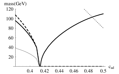
In the region , all of these masses are monotonically decreasing function of . When , we obtain . Thus and vanish in this region. The mass of the Higgs also decreases with increasing for larger as long as . For , however, the mass of Higgs increases and closes to , because the contribution from the top quark becomes dominant in this region.
So that GeV and GeV satisfy the relation (88), is required. This value of is, however, smaller than the lower bound which is obtained by solving Wilson-line dynamics. Furthermore, it seems unlikely to push up (down) the () just by introducing more adjoint fermions, because the minimum of the locates at and we cannot make smaller than only by introducing more adjoint fermion into the model. In the following subsections we try to push up (down) (), by adding some scalar fields or twisted fermions.
III.3 Adding Scalar Fields
The action of a bulk scalar field can be written as GP
| (89) |
where and are the bulk and boundary mass of the scalar field , respectively.1010 10 For simplicity, we do not include scalar quartic terms. Therefore, we do not consider the case in which the scalar fields develop VEVs and cause Higgs mechanism here. The cases in which the Higgs mechanism and the dynamical gauge-Higgs unification coexist are discussed in Sakamoto_gauge-higgs. When and satisfy the relation:
| (90) |
the KK-mass spectrum of such scalar becomes identical to a fermion field with the bulk mass , and the contribution to the effective potential par degrees of freedom turns out to be just same magnitude but with opposite sign as the one from the fermion in the same representation of . Hereafter we consider the case where boundary- and bulk-masses of scalar fields satisfy the condition (90).
Now we propose a way to lift up (put down) the -boson mass () by introducing scalar fields into the model. We add one or more scalar fields (, ), which are in the fundamental representation of , into the model. The contribution to the effective potential from such scalar fields is given as
| (91) |
where () are mass parameters of the scalar and related with the boundary and bulk mass parameters , by and . The total effective potential is given by . For simplicity, we use an approximation of Eq. (91), which is given by
| (92) |
where we have introduced a dimensionless parameter , . Since has the global minimum at , we can shift the location of the minimum of to by increasing the value of . Thus in this model we can change the ratio by tuning adjoint fermion mass and the scalar field contribution parameterized by . In FIG. 7(a) and (b), we have shown how depends on .


FIG. 7 tells that can be achieved by tuning for any value of . Thus for a given value of , we can define such that has the global minimum at with . In TABLE. 2, we summarized the value of for each value of . And we re-calculate masses , with and .
| [GeV] | ||||||
|---|---|---|---|---|---|---|
| [GeV] | ||||||
| [GeV] |
The KK-scale and the first KK-photon mass at are GeV and GeV, respectively.
One may wonder why the Higgs mass becomes larger nevertheless scalar field may cancel the fermion’s contribution. The reason can be explained as follows. First, we remember that and have similar shape to and , respectively. Then the contribution of the adjoint fermion to the Higgs mass (i.e. the curvature of ) has the maximum around at , whereas one of fundamental scalars vanishes at . Thus the Higgs mass becomes small when the closes to .
III.4 Twisted Fermion
An alternative way to shift the Z-boson mass in the model is to introduce one or more “twisted fermions” , which boundary condition is twisted even in AB-gauge. As an example, we consider the case where is in the fundamental representation of . As a possible boundary condition of in the AB-gauge, we define
| (93) | |||
| (94) |
where is defined in (59) and . When we introduce copies of such twisted-fermions () with into the model, the contribution to the one-loop effective potential induced from such fermions is given by
| (95) |
where is the bulk mass parameter of . Since , we can make use of the result of Sec. III.3 by replacing in (92) with and with .
IV Summary and Comments
In the present paper, we investigated the dynamical gauge-Higgs unification in the RS space-time. In Sec. II we consider the SU(2) gauge theory in the RS space-time. We calculate one-loop effective potential with respect to the Wilson-line phase. Especially we clarified the contribution from a fermion with the bulk mass parameter . The obtained effective potential properly inter/extrapolates the results which are known for . We see that the gauge symmetry can be broken by dynamically-induced Wilson line when we introduce an adjoint fermion into the model and that the breaking pattern of the gauge symmetry depends on the bulk mass of the adjoint fermion.
In Sec.III we consider gauge models in the RS as toy models of 5D extensions of the electroweak theory. We found that it is possible to break to by introducing an adjoint fermion. The large mass hierarchy among quarks and leptons are naturally obtained by adjusting their bulk mass parameters of the order of unity. We calculate one-loop Higgs mass numerically. In the model the Higgs mass can be changed from zero to with . We have also estimated mass spectrum of this model for various value of mass of the adjoint fermion, which are determined by the RS parameter and bulk mass parameter of the adjoint fermion. Interestingly, these predicted masses of Higgs and new fermions are in the range where LHC experiment can explore. In this model, we see that the ratio of -boson mass to the -boson mass varies with respect to the Wilson-line phase. This occurs at tree level. We find the way to tune the ratio to satisfy the realistic one , by introducing fundamental scalar fields with the bulk and boundary mass terms which satisfy the relation (90), or fermions with twisted boundary condition. Unfortunately, the model still has some problems, e.g., varying may occur due to the lack of custodial symmetry in this model, some SM and non-SM fermions remain massless, and quarks and leptons cannot have correct isospin and hypercharge simultaneously. To obtain a more realistic model of the EWGHU in the RS space-time, the choice of the enhanced electroweak symmetry and the assignment of matter contents should be reconsidered.
We have seen that in the model a quark with small bulk masses has a heavy lowest KK state1111 11 It is not true in the case of flat extra dimension, where a fermion with large bulk mass tends to have large lowest KK mass., and that such heavy fermions have large contribution to the effective potential of Higgs because of the smallness of bulk masses. The converse is also true; fermions with large bulk mass term have light lowest KK masses and have small contributions to the effective potential. It remind us the qualitative similarity with the CW mechanism; In CW mechanism the contribution to the Higgs potential from a heavy quark loop is large because a heavy fermion has large Yukawa coupling to the Higgs field. However, we have to note that in the dynamical gauge-Higgs unification the quadratic divergence of Higgs mass is absent, thanks to the gauge symmetry in the higher-dimensional space-time.
Acknowledgements.
Author will thank Darwin Chang for fruitful discussion. This work was initiated during author’s stay at National Tsing-Hua University. Author also thanks National Center for Theoretical Science in Hsinchu for warm hospitality. This work is partly supported by National Science Council of R.O.C. under Grant No. 93-2112-M-007-015.Appendix A Approximation Formulas
When the 4D (or lowest KK mode) mass of a field is sufficiently smaller than , i.e., , we can use an approximation formula for , as discussed in Hosotani06. The mass is approximated by
| (96) |
where is defined by
| (97) |
The mass of the weak boson is give by , and can be approximated by1212 12 Here we have taken the limit: .
| (98) |
From Eqs. (97),(98), the lowest KK mass is also approximated (in terms of ) by
| (99) |
where is defined by
| (100) | |||||
Here we should note that is independent of the .
As for , by using -mass formula (98) inversely we obtain
| (101) |
We should also note that Eq. (97) is an approximation of and valid valid only when . When close to , the difference between and becomes large (see FIG. 8).

References
- (1) N. S. Manton, Nucl. Phys. B 158, 141 (1979).
- (2) D. B. Fairlie, Phys. Lett. B 82, 97 (1979).
- (3) N. V. Krasnikov, Phys. Lett. B 273, 246 (1991).
- (4) Y. Hosotani, Phys. Lett. B 126, 309 (1983); Y. Hosotani, Phys. Lett. B 129, 193 (1983).
- (5) E. Witten, Nucl. Phys. B 258, 75 (1985).
- (6) Y. Hosotani, Annals Phys. 190, 233 (1989).
- (7) N. Haba, M. Harada, Y. Hosotani and Y. Kawamura, Nucl. Phys. B 657, 169 (2003) [Erratum-ibid. B 669, 381 (2003)] [arXiv:hep-ph/0212035]; N. Haba, Y. Hosotani and Y. Kawamura, Prog. Theor. Phys. 111, 265 (2004) [arXiv:hep-ph/0309088]; N. Haba and T. Yamashita, JHEP 0402, 059 (2004) [arXiv:hep-ph/0401185]; N. Haba, Y. Hosotani, Y. Kawamura and T. Yamashita, Phys. Rev. D 70, 015010 (2004) [arXiv:hep-ph/0401183]. N. Haba and T. Yamashita, JHEP 0402, 059 (2004) [arXiv:hep-ph/0401185]; JHEP 0404, 016 (2004) [arXiv:hep-ph/0402157].
- (8) I. Antoniadis, Phys. Lett. B 246, 377 (1990).
- (9) N. Arkani-Hamed, S. Dimopoulos and G. R. Dvali, Phys. Lett. B 429, 263 (1998) [arXiv:hep-ph/9803315].
- (10) H. Hatanaka, T. Inami and C. S. Lim, Mod. Phys. Lett. A 13, 2601 (1998) [arXiv:hep-th/9805067].
- (11) L. J. Hall, Y. Nomura and D. R. Smith, Nucl. Phys. B 639, 307 (2002) [arXiv:hep-ph/0107331].
- (12) I. Antoniadis, K. Benakli, Act. Phys. Polon. B 33, 2477 (2002)
- (13) K. w. M. Choi, N. y. M. Haba, K. S. M. Jeong, K. i. M. Okumura, Y. Shimizu and M. Yamaguchi, JHEP 0402, 037 (2004) [arXiv:hep-ph/0312178].
- (14) C. A. Scrucca, M. Serone, L. Silvestrini and A. Wulzer, JHEP 0402, 049 (2004) [arXiv:hep-th/0312267]; G. Panico and M. Serone, JHEP 0505, 024 (2005) [arXiv:hep-ph/0502255]. G. Panico, M. Serone and A. Wulzer, Nucl. Phys. B 739, 186 (2006) [arXiv:hep-ph/0510373]; G. Panico, arXiv:hep-ph/0610366.
- (15) I. Antoniadis, K. Benakli and M. Quiros, New J. Phys. 3, 20 (2001) [arXiv:hep-th/0108005].
- (16) M. Kubo, C. S. Lim and H. Yamashita, Mod. Phys. Lett. A 17, 2249 (2002) [arXiv:hep-ph/0111327].
- (17) Y. Hosotani, S. Noda and K. Takenaga, Phys. Lett. B 607, 276 (2005) [arXiv:hep-ph/0410193].
- (18) N. Maru and K. Takenaga, Phys. Lett. B 637, 287 (2006) [arXiv:hep-ph/0602149]; Phys. Rev. D 74, 015017 (2006) [arXiv:hep-ph/0606139].
- (19) C. Csaki, C. Grojean and H. Murayama, Phys. Rev. D 67, 085012 (2003) [arXiv:hep-ph/0210133].
- (20) B. Grzadkowski and J. Wudka, Phys. Rev. Lett. 97, 211602 (2006) [arXiv:hep-ph/0604225].
- (21) N. Maru and T. Yamashita, Nucl. Phys. B 754, 127 (2006) [arXiv:hep-ph/0603237]; Y. Hosotani, N. Maru, K. Takenaga and T. Yamashita, arXiv:0709.2844 [hep-ph]; Y. Hosotani, arXiv:hep-ph/0607064.
- (22) N. Haba, K. Takenaga and T. Yamashita, Phys. Lett. B 615, 247 (2005) [arXiv:hep-ph/0411250].
- (23) M. Sakamoto and K. Takenaga, Phys. Rev. D 75, 045015 (2007) [arXiv:hep-th/0609067].
- (24) G. Cacciapaglia, C. Csaki and S. C. Park, JHEP 0603, 099 (2006) [arXiv:hep-ph/0510366].
- (25) H. Hatanaka, Prog. Theor. Phys. 102, 407 (1999) [arXiv:hep-th/9905100]; N. Haba, K. Takenaga and T. Yamashita, Phys. Lett. B 605, 355 (2005) [arXiv:hep-th/0410244]; N. Maru and K. Takenaga, Phys. Rev. D 72, 046003 (2005) [arXiv:hep-th/0505066]; M. Serone, G. Panico, arXiv:hep-ph/0511348; M. Salvatori, arXiv:hep-ph/0611309; C. S. Lim, N. Maru and K. Hasegawa, arXiv:hep-th/0605180; N. Irges et al. Nucl. Phys. B 775, 283 (2007) [arXiv:hep-lat/0609045]; JHEP 0708, 028 (2007) [arXiv:0706.3806 [hep-ph]], arXiv:0709.4549 [hep-lat]; C. T. Hill and R. J. Hill, arXiv:hep-ph/0701044; C. S. Lim and N. Maru, Phys. Rev. D 75, 115011 (2007) [arXiv:hep-ph/0703017], Phys. Lett. B 653, 320 (2007) [arXiv:0706.1397 [hep-ph]]; Y. Adachi, C. S. Lim and N. Maru, Phys. Rev. D 76, 075009 (2007) [arXiv:0707.1735 [hep-ph]]; N. Maru and N. Okada, arXiv:0711.2589 [hep-ph]; N. Cosme et al. Phys. Rev. D 68, 096001 (2003) [arXiv:hep-ph/0207024]; Phys. Rev. D 69, 036003 (2004) [arXiv:hep-ph/0303037]; B. Grzadkowski and J. Wudka, Phys. Rev. Lett. 93, 211603 (2004) [arXiv:hep-ph/0401232]; Phys. Rev. D 72, 125012 (2005) [arXiv:hep-ph/0501238]; D. Chang, C. S. Chen, C. H. Chou and H. Hatanaka, Phys. Rev. D 70, 096010 (2004) [arXiv:hep-ph/0406059]; N. Haba, S. Matsumoto, N. Okada and T. Yamashita, JHEP 0602, 073 (2006) [arXiv:hep-ph/0511046]; l. Gogoladze, N. Okada and Q. Shafi, arXiv:0705.3035 [hep-ph], arXiv:0708.2503 [hep-ph]. S. Randjbar-Daemi and V. Rubakov, arXiv:0709.1202 [hep-ph].
- (26) M. R. Carter, Phys. Rev. D 36, 412 (1987); G. Burdman and Y. Nomura, Nucl. Phys. B 656, 3 (2003) [arXiv:hep-ph/0210257]; N. Haba and Y. Shimizu, Phys. Rev. D 67, 095001 (2003) [Erratum-ibid. D 69, 059902 (2004)] [arXiv:hep-ph/0212166]; I. Gogoladze et al. Phys. Lett. B 560, 204 (2003) [arXiv:hep-ph/0301014], Phys. Lett. B 649, 212 (2007) [arXiv:hep-ph/0703107].
- (27) A. Higuchi and L. Parker, Phys. Rev. D 37, 2853 (1988); A. T. Davies and A. McLachlan, Phys. Lett. B 200, 305 (1988).
- (28) S. R. Coleman and E. Weinberg, Phys. Rev. D 7, 1888 (1973).
- (29) L. Randall and R. Sundrum, Phys. Rev. Lett. 83, 3370 (1999) [arXiv:hep-ph/9905221].
- (30) A. Flachi, I. G. Moss and D. J. Toms, Phys. Rev. D 64, 105029 (2001) [arXiv:hep-th/0106076].
- (31) K. y. Oda and A. Weiler, Phys. Lett. B 606, 408 (2005) [arXiv:hep-ph/0410061].
- (32) A. D. Medina, N. R. Shah and C. E. M. Wagner, arXiv:0706.1281 [hep-ph].
- (33) Y. Hosotani and M. Mabe, Phys. Lett. B 615, 257 (2005) [arXiv:hep-ph/0503020].
- (34) Y. Hosotani, S. Noda, Y. Sakamura and S. Shimasaki, Phys. Rev. D 73, 096006 (2006) [arXiv:hep-ph/0601241].
- (35) Y. Hosotani and Y. Sakamura, Phys. Lett. B 645, 442 (2007) [arXiv:hep-ph/0607236]; Y. Hosotani and Y. Sakamura, arXiv:hep-ph/0703212; Y. Sakamura, Phys. Rev. D 76, 065002 (2007) [arXiv:0705.1334 [hep-ph]];
- (36) R. Contino, Y. Nomura and A. Pomarol, Nucl. Phys. B 671, 148 (2003) [arXiv:hep-ph/0306259]; K. Agashe, R. Contino and A. Pomarol, Nucl. Phys. B 719, 165 (2005) [arXiv:hep-ph/0412089]; K. Agashe and R. Contino, Nucl. Phys. B 742, 59 (2006) [arXiv:hep-ph/0510164]; A. Falkowski, Phys. Rev. D 75, 025017 (2007) [arXiv:hep-ph/0610336], arXiv:0710.4050 [hep-ph]; M. S. Carena, E. Ponton, J. Santiago and C. E. M. Wagner, Phys. Rev. D 76, 035006 (2007) [arXiv:hep-ph/0701055]; G. Panico and A. Wulzer, JHEP 0705, 060 (2007) [arXiv:hep-th/0703287]; . D. Green, A. Lawrence, J. McGreevy, D. R. Morrison and E. Silverstein, Phys. Rev. D 76, 066004 (2007) [arXiv:0705.0550 [hep-th]].
- (37) H. C. Cheng, C. T. Hill and J. Wang, Phys. Rev. D 64, 095003 (2001) [arXiv:hep-ph/0105323]; T. Kobayashi, N. Maru and K. Yoshioka, Eur. Phys. J. C 29, 277 (2003) [arXiv:hep-ph/0110117]; A. Falkowski and H. D. Kim, JHEP 0208, 052 (2002) [arXiv:hep-ph/0208058]; L. Randall, Y. Shadmi and N. Weiner, JHEP 0301, 055 (2003) [arXiv:hep-th/0208120]; J. de Blas, A. Falkowski, M. Perez-Victoria and S. Pokorski, JHEP 0608, 061 (2006) [arXiv:hep-th/0605150]; H. C. Cheng, J. Thaler and L. T. Wang, JHEP 0609, 003 (2006) [arXiv:hep-ph/0607205].
- (38) Y. Grossman and M. Neubert, Phys. Lett. B 474, 361 (2000) [arXiv:hep-ph/9912408].
- (39) H. Davoudiasl, J. L. Hewett and T. G. Rizzo, Phys. Rev. D 63, 075004 (2001) [arXiv:hep-ph/0006041]; H. Davoudiasl, J. L. Hewett and T. G. Rizzo, Phys. Lett. B 473, 43 (2000) [arXiv:hep-ph/9911262]; S. J. Huber and Q. Shafi, Phys. Rev. D 63, 045010 (2001) [arXiv:hep-ph/0005286]; B. Batell and T. Gherghetta, Phys. Rev. D 75, 025022 (2007) [arXiv:hep-th/0611305].
- (40) T. Gherghetta and A. Pomarol, Nucl. Phys. B 586, 141 (2000) [arXiv:hep-ph/0003129].
- (41) S. Chang, J. Hisano, H. Nakano, N. Okada and M. Yamaguchi, Phys. Rev. D 62, 084025 (2000) [arXiv:hep-ph/9912498]; S. Chang, S. C. Park and J. Song, Phys. Rev. D 71, 106004 (2005) [arXiv:hep-ph/0502029].
- (42) J. M. Maldacena, Adv. Theor. Math. Phys. 2, 231 (1998) [Int. J. Theor. Phys. 38, 1113 (1999)] [arXiv:hep-th/9711200].
- (43) N. Arkani-Hamed, A. G. Cohen and H. Georgi, Phys. Rev. Lett. 86, 4757 (2001) [arXiv:hep-th/0104005]; Phys. Lett. B 513, 232 (2001) [arXiv:hep-ph/0105239]; H. C. Cheng, C. T. Hill, S. Pokorski and J. Wang, Phys. Rev. D 64, 065007 (2001) [arXiv:hep-th/0104179].
- (44) W. D. Goldberger and M. B. Wise, Phys. Rev. Lett. 83, 4922 (1999) [arXiv:hep-ph/9907447].
- (45) S. J. Huber, Nucl. Phys. B 666, 269 (2003) [arXiv:hep-ph/0303183]; K. Agashe, G. Perez and A. Soni, Phys. Rev. D 71, 016002 (2005) [arXiv:hep-ph/0408134]; B. Lillie, L. Randall and L. T. Wang, JHEP 0709, 074 (2007) [arXiv:hep-ph/0701166]; H. Davoudiasl and A. Soni, arXiv:0705.0151 [hep-ph].
- (46) J. Garriga, O. Pujolas and T. Tanaka, Nucl. Phys. B605 192(2001); W. D. Goldberger and I. Z. Rothstein, Phys. Lett. B491 339(2000).
- (47) Y. Aharonov and D. Bohm, Phys. Rev. 115, 485 (1959).
- (48) R. Barate et al. [LEP Working Group for Higgs boson searches], Phys. Lett. B 565, 61 (2003) [arXiv:hep-ex/0306033].
- (49) H. Hatanaka, K. Ohnishi, M. Sakamoto and K. Takenaga, Prog. Theor. Phys. 107, 1191 (2002) [arXiv:hep-th/0111183]; Prog. Theor. Phys. 110, 791 (2003) [arXiv:hep-th/0305213].