Spectrum of the non-abelian phase in Kitaev’s honeycomb lattice model
Abstract
The spectral properties of Kitaev’s honeycomb lattice model are investigated both analytically and numerically with the focus on the non-abelian phase of the model. After summarizing the fermionization technique which maps spins into free Majorana fermions, we evaluate the spectrum of sparse vortex configurations and derive the interaction between two vortices as a function of their separation. We consider the effect vortices can have on the fermionic spectrum as well as on the phase transition between the abelian and non-abelian phases. We explicitly demonstrate the -fold ground state degeneracy in the presence of well separated vortices and the lifting of the degeneracy due to their short-range interactions. The calculations are performed on an infinite lattice. In addition to the analytic treatment, a numerical study of finite size systems is performed which is in exact agreement with the theoretical considerations. The general spectral properties of the non-abelian phase are considered for various finite toroidal systems.
Keywords:
Topological models, Non-abelian vortices, Kitaev’s modelPACS
05.30.Pr, 75.10.Jm1 , 2, 3, 4, 2 and 1
1 Introduction
Topological quantum computation [1, 2, 3, 4] is certainly among the most exotic proposals for performing fault-tolerant quantum information processing. This approach has attracted considerable interest, since it is closely related to the problem of classifying topologically ordered phases in various condensed matter systems. The connection is provided by anyonic quasiparticles, which appear as states of topologically ordered systems with non-trivial statistical properties. Some of these anyon models can support universal quantum computation. Up to now, no complete classification of topological phases exists in terms of their physical properties or their computational power. This is due to the small number of analytically treatable models that exhibit topological behavior. The most studied arena is the celebrated fractional Quantum Hall effect [5, 6] appearing in a two dimensional electron gas when it is subject to a perpendicular magnetic field.
Recently various two dimensional lattice models exhibiting topological behavior have been proposed [7, 8, 9, 10, 11, 12, 13] that enjoy analytic tractability. One such lattice proposal is the honeycomb model introduced by Alexei Kitaev [10]. It consists of a two dimensional honeycomb lattice with spins at its vertices subject to highly anisotropic spin-spin interactions. This model has several remarkable features. It is exactly solvable and can thus be studied analytically. For particular values of the couplings, the model can be mapped to gauge theory on a square lattice (the toric code), which supports abelian anyons. This anyon model has been employed for performing various quantum information tasks [2]. When one adds an external magnetic field, the model supports non-abelian Ising anyons. Even though neither model supports universal quantum computation, particular variations of the latter have been considered for this purpose [14, 15]. One expects that when the couplings of the honeycomb lattice model are varied, the system will undergo a phase transition between the abelian and non-abelian phases. The existence of the different phases is only argued in the original work [10] based on mathematical considerations and no rigorous presentation of the transition is provided.
So far, the studies on Kitaev’s honeycomb lattice model have concentrated on the abelian phase [16, 17, 18]. Here we present an extensive study of its spectral properties in the presence of an external magnetic field. Solving the model for various sparse vortex configurations gives us qualitative and quantitative results for the behavior of the spectrum in the non-abelian phase. The study includes the explicit demonstration of zero modes in the presence of well separated vortices and the lifting of the degeneracy due to their short-range interaction. These properties are subsequently connected to the properties of the Ising anyon model giving direct evidence that the low energy behavior of the non-abelian phase is indeed captured by this model. In addition, we consider the stability of the different phases, which is of importance when one is interested in physically realizing the model [19]. The analytic calculations are supported by exact numeric diagonalizations of finite size systems. The exact agreement between the analytic and numeric solutions for these finite size systems is demonstrated and the effect of an external effective magnetic field on finite size systems is discussed. Our work generalizes the analysis in [17] performed by one of the authors, where only the abelian phases in the limiting vortex-free and full-vortex cases were considered.
The paper is organized as follows. In Section 2 we give an overview of the honeycomb lattice model. There we outline the analytic approach for solving the model for various vortex configurations by employing Majorana fermionization. Section 3 provides explicitly the analytic solution for the limiting cases of vortex-free and full-vortex configurations. These calculations are subsequently generalized to sparse vortex configurations. Section 4 forms the main body of our work. There we analyze in detail the behavior of the spectrum in different parts of the phase space and study how it is modified due to the presence of vortices. A connection to the Ising anyon model is provided. In Section 5 we study exact numerical diagonalization of various finite size systems and show the equivalence with the analytic results. Final remarks and conclusions are given in Section 6.
2 The spectrum of arbitrary vortex configurations
2.1 The honeycomb lattice model
We briefly review here the honeycomb lattice model and its analytical treatment as described in [10]. The model is defined on a honeycomb lattice with spins residing at each site. The sites are bi-colored black and white such that , where and are two triangular sublattices.

We shall consider the following Hamiltonian
| (1) |
where and are positive coupling strengths along the -, - and -links, respectively, as shown in Figure 1(a). The three-spin interaction, or the -term, on the right hand side can be obtained from a perturbative expansion when we apply a weak (Zeeman) magnetic field of the form . In this case is given by , and this model is assumed to approximate the one with a Zeeman term when . Only this third order term in the perturbative expansion will be of interest to us, since it is the lowest order term breaking time reversal invariance [10]. The summations in the effective magnetic field term run over site triples such that every plaquette contributes the six terms
| (2) |
The sites of a single plaquette have been enumerated as shown in Figure 1(b). The Hamiltonian (1) commutes with the plaquette operators defined by
| (3) |
where the product is taken over all plaquettes of a compact lattice and is the identity operator. The eigenvalue is interpreted as having a vortex on plaquette . The constraint in (3) implies that the vortices always come in pairs. Since are conserved quantities, one can fix the underlying vortex configuration and consider the Hamiltonian over this sector. This would not be possible when the usual Zeeman term were employed, since it does not commute with the plaquette operators. Thus, the magnetic field induces hopping of the vortices between neighboring plaquettes and their number is not necessarily conserved.
The Hamiltonian can be diagonalized by representing the spin operators with Majorana fermions. Following [10, 17] we introduce two fermionic modes and residing at each lattice site. The corresponding Majorana fermions are given by
| (4) |
We encode the spin at each site at the subspace where both of the fermionic modes are either empty or full. In terms of the four Majorana fermions, this means that we need to project down to a two dimensional subspace, the physical space , by employing the projector , i.e. . The representation of the spin matrices at site is then given in terms of the Majorana fermions by , which satisfy the Pauli algebra when restricted in (note that ). It follows that
| (5) |
where we have defined the operators
| (6) |
with depending whether and are connected by a -, - or -link, respectively. Consequently, Hamiltonian (1) takes the form
| (7) |
The explicit appearance of the constraint in (5) has been omitted, as we consider only operations in the physical subspace . The couplings are given by or . The summations in the Hamiltonian (7) are most conveniently expressed pictorially (see Figure 1(c)). The solid lines correspond to nearest neighbor (the first term of in (7)) and the dashed lines to next to nearest neighbor summation (the second term of in (7)). The antisymmetry of the ’s in (6) is taken into account by using a convention such that one assigns an overall () to every term involving sites and when the arrow points from to ( to ). If two sites are not connected by an arrow the corresponding element is zero.
The plaquette operators (3) can be written in terms of the ’s as
| (8) |
where denotes the boundary of plaquette . Also, one can check that . These observations imply that after performing the fermionization, the underlying vortex configuration can be fixed by specifying the eigenvalues of the operators on every link of the model. The eigenvalue means that there is a string passing through the link that either connects two vortices or belongs to a loop. The locations of these vortices are determined by the eigenvalues of the plaquette operators.
2.2 Solution for periodic vortex configurations
Let us now consider in more detail the form of Hamiltonian (7) for various periodic vortex configurations and its diagonalization by using Fourier transform. Without affecting the physics of our system we shall deform the original honeycomb lattice to a square lattice by taking the length of -links to zero and choosing the lattice basis vectors to be and . The resulting square lattice is shown in Figure 2.
First we determine the unit cell of our periodic vortex lattice. The simplest possible choice contains a -link of the honeycomb lattice, or in other words a single site on the square lattice. We refer to this choice of unit cell as the elementary cell.

In order to employ Fourier transform in diagonalizing the Hamiltonian the underlying vortex configuration must be periodic with respect to the choice of the unit cell. For the elementary cell there is only one such configuration - the vortex-free configuration [10]. The full-vortex configuration, i.e. a vortex on every plaquette, can be solved by taking two elementary cells in which alternates its sign along one direction [17]. However, our aim is to go beyond these two limiting cases and consider arbitrary sparse vortex configurations. To do this, we define a generalized -unit cell, which contains elementary cells. On the square lattice the basis vectors take the simple form
| (9) |
An arbitrary site on the original honeycomb lattice can be labeled by the triplet , where is a vector indicating the location of the unit cell, the index pair specifies a particular elementary cell inside the generalized unit cell and is an index specifying whether the site belongs to or . If denotes the number of unit cells, there are altogether sites on the lattice.
Using this notation the Hamiltonian (7) can be written as
| (10) |
where the vector is summed over all linear combinations of the lattice basis vectors (9). Since , the operators (6) appearing in (7) have been replaced with their eigenvalues . The antisymmetry of the operators is included in the summation convention (Figure 1(c)). The properly normalized Fourier transformation of the operators is given by
| (11) |
Substituting this into (10) we obtain the canonical form
where , and are matrices with elements . This Hamiltonian is a generalization of the one obtained in [10] with the exception that the single entries of the Hamiltonian are replaced here with matrices.
The off-diagonal blocks correspond to nearest-neighbor interactions. The non-vanishing elements of the Hamiltonian for arbitrary -unit cells are given by
where the addition in the indices is understood and for and otherwise. The diagonal blocks correspond to next-to-nearest neighbor couplings and are given by
where we have used the short-hand notation . Both and are Hermitian, which can be checked by taking first Hermitian conjugates and subsequently shifting the indices accordingly. Likewise, one can check the relations,
| (41) |
that guarantee the Hermiticity of .
The expressions derived above give the most general expression for the Hamiltonian of the honeycomb lattice model. To proceed with the diagonalization, one needs to specify the underlying vortex configuration, i.e. the values of on each link. Since all bi-colorable Hamiltonians have a double spectrum [10], we know that the diagonalization of (2.2) will give the general form
| (42) |
where are fermionic operators and are functions to be determined. The latter correspond to the eigenvalues of the matrix . Their exact form has to be calculated separately for each choice of unit cell and vortex configuration. The ground state and the first excited state corresponding to a particular vortex configuration are given by
| (43) |
where is a state with no Majorana fermions and is the momentum minimizing the lowest lying eigenvalue , i.e. . It follows that the corresponding total ground state energy, , and the fermion gap, , are given by
| (44) | |||||
| (45) |
3 Analytic results at the thermodynamic limit
In this section we present analytic solutions to the two limiting vortex configurations: the vortex-free and full-vortex configurations. Furthermore, we outline how the generalized unit cells can be used to study configurations, where the separation between two vortices is varied. This will be later used to study the behavior of the relative ground state energies and fermion gaps as the function of the vortex separation.
3.1 The vortex-free configuration
The vortex-free configuration is achieved by setting
| (46) |
This configuration is periodic with respect to each -link and thus we can choose a -unit cell (see Figure 3(a)). The off-diagonal, (2.2), and diagonal, (2.2), elements are then given by
Inserting these together with (41) into (2.2), we obtain a Hamiltonian which is diagonalized by introducing the fermionic operator
where
The eigenvalues of the Hamiltonian are given by , and thus the total ground state energy (44) and the fermion gap (45) are given by
| (47) | |||||
| (48) |
These results agree with the ones obtained in [10] and [17].
 |
 |
| (a) | (b) |
3.2 The full-vortex configuration
The full-vortex configuration can be obtained by choosing a -unit cell and setting
Figure 3(b) illustrates the choice of unit cell for this case. Equations (2.2) and (2.2) become
and
Inserting these into (2.2) and diagonalizing the resulting Hamiltonian we obtain the eigenvalues
| (58) |
where
The analytic expressions of the corresponding eigenvectors are not presented here as they are too lengthy. When we set our results agree with the analytic calculations performed in [17] in the absence of the -term. The total ground state energy (44) is now given by
| (59) |
and the fermionic gap (45) becomes
| (60) |
3.3 Sparse vortex configurations
We turn next to sparse vortex configurations in order to study the interactions between vortices. This is done by considering how the ground state energies and fermion gaps of 2-vortex configurations behave when the separation between vortices is varied. A configuration with two vortices separated by plaquettes is created, for instance, by selecting an -unit cell and setting
Assuming , vortex separations of can be studied.
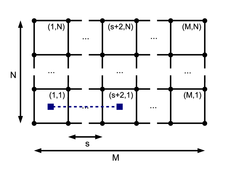
Figure 4 illustrates the unit cell and the resulting vortex configuration. Since we are working on an infinite plane, ideally one would like to use a unit cell of infinite size in order to isolate the interaction between the vortices. However, the Hamiltonian (2.2) grows polynomially in and and hence we restrict to considering a -unit cell. This choice allows separations , which is shown later to be sufficient to extract the expected asymptotic behavior when . The resulting Hamiltonians are sparse matrices, which can not be treated analytically, but can be diagonalized numerically in a reasonable time using a tabletop computer. Using (44) and (45) we can then calculate the total ground state energies and fermion gaps corresponding to 2-vortex configurations with vortex separation .
4 Analysis of the spectrum
The spectrum of Hamiltonian (1) can be characterized by two different types of energy gaps: fermionic gaps that characterize the energy levels of the spectrum above a fixed vortex configuration and vortex gaps that compare the ground state energies corresponding to different vortex configurations. We determine how the presence of vortices influences the fermionic gaps and, subsequently, how the phase space geometry is modified. We also determine the scaling of the ground state degeneracy, which is expected due to the presence of the Ising non-abelian vortices. Moreover, we carry out a study on the 2-vortex configuration energies as a function of the vortex separation, and subsequently determine the vortex gap, i.e. the energy required to excite a pair of free vortices.
4.1 The fermion gap
4.1.1 The phase space geometry in the presence of vortices
First, we briefly review the phase space of the vortex-free sector, which was studied in [10]. It was shown that the honeycomb lattice model exhibits four distinct phases and for different values of the couplings such that the system is in the -phase when all the inequalities , and are violated. The phase boundaries are given by the equalities and the phase occurs when only holds and the other two inequalities are violated. The phases are always gapped for , and the vortices behave as abelian anyons. On the other hand, the -phase is gapped only when and only there the vortices behave as non-abelian Ising anyons. The phase boundaries are the lines in the phase space where the fermion gap vanishes. Here we restrict to studying the transition, i.e. the behavior of the fermion gap between the (abelian) and the (non-abelian) phases. Figure 5 illustrates the general phase space geometry where we’ve taken . For convenience we normalize from now on the couplings such that and .

 |
 |
| (a) | (b) |
Figures 6(a) and 6(b) show the vortex-free, (48), and full-vortex, (60), fermionic gaps plotted as functions of for different values of . Let us first consider the case. In the vortex-free configuration the gap vanishes at , in agreement with [10]. In the full-vortex configuration the gap persists till in line with the results derived in [17]. There the phase boundary equalities for the full-vortex configuration were derived to take the form . When , in both cases the fermion gaps reappear and settle at a constant value once the system moves well into the phase. However, the dependence of the gap magnitude on is clearly different for the vortex-free and full-vortex configurations with the gap being much smaller in the latter case. Also, Figure 6(b) shows that at the transition between the phases is shifted away from . This implies that the magnitude of can also affect the phase space geometry.
In the limiting cases we observe that the boundary between the two phases depends on the underlying vortex configuration. To study how the fermionic energy gap interpolates in between these two extreme cases, we consider the fermion gaps of various sparse vortex configurations on small unit cells. In all the cases the phase boundary falls into the region when . For very sparse configurations with low vortex density such as the 2-vortex configuration created by (3.3), the boundary is located very close to , whereas for more homogeneously distributed configurations with larger vortex density it tends towards . However, when the phase boundary is in general shifted to larger ’s such that for some configurations the boundary is located in the area . We attribute the shifting of the phase boundary to short-range vortex-vortex interactions, which are enhanced when is increased. It is interesting to note that since the vortex density affects the phase space geometry in the region and , it could, in principle, be used as a tunable parameter, that induces a phase transition between the abelian and non-abelian phase.
4.2 The fermion gap in the presence of vortices
It is intriguing to study the behavior of the fermionic gap in the presence of only two vortices as a function of their distance. For that we consider again the 2-vortex configurations with varying vortex separation , which are created by setting the ’s as given by (3.3). Figure 7(a) shows the behavior of the corresponding fermion gap as the function of in the abelian and in the non-abelian phase for several values of . The behavior in the different phases is radically different. In the abelian phase the fermion gap is in practice insensitive to both and . In stark contrast to the abelian phase, the fermion gap in the non-abelian phase decreases exponentially with vanishing completely for .11 1 The oscillations of the energy gap as a function of the vortex separation appear to be Friedel oscillations. Indeed, in Figure 7(b) we plot the gaps to the two first excited states,
and observe that tends exponentially to zero as increases with the value at being of order . This means that in the presence of two well separated vortices the ground state of the non-abelian phase is twofold degenerate. Moreover, the gap to the second excited state, , is found to be insensitive to and persist to arbitrary separations.
 |
 |
| (a) | (b) |
 |
 |
| (a) | (b) |
It is known that the honeycomb lattice model can be mapped to a -wave superconductor where the fermions live on the -links [16, 25]. The vortices in the superconductor are assumed to be non-abelian Ising anyons [6], which are also predicted to appear as vortices in the honeycomb lattice model [10]. In the presence of well separated vortices the ground state should be -fold degenerate, but when vortices are brought together, their interactions are predicted to lift the degeneracy [6, 20, 24]. Our demonstration of the twofold degenerate ground state in the presence of two vortices is in agreement with this prediction. To verify that the degeneracy scales as for the honeycomb lattice model, we consider in addition 4- and 6-vortex pairwise configurations where the vortex pairs are located on equally spaced rows of the -unit cell and the separation of the vortices from each pair is simultaneously varied. In the 4-vortex case the fermion gaps to the four first excited states are given by
Similarly, the gaps to the eight first excited states for the 6-vortex configuration are
Figures 8(a) and (b) depict the behavior of the 4- and 6-vortex configuration fermion gaps (4.2) and (4.2), respectively, at and as a function of . The degeneracy of the ground state as is four for 4-vortex and eight for 6-vortex configurations. This is exactly the predicted scaling. We also observe that at the interaction does not completely lift the degeneracies. The ground state becomes non-degenerate for small , but some of the states form degenerate bands. The splitting in energy between the bands is homogenous in the sense that for a specific it costs the same amount of energy to move between the shifted states. We also observe that for all the considered vortex configurations the first non-vanishing gap as is always two units of energy above the ground state. As can be seen from Figure 6(a), this is the case also for the vortex-free fermion gap, , at and . The observation suggests that the energy to excite a fermionic mode is insensitive to the underlying vortex configuration and depends only on and . We will adopt to denote the energy to create a free fermionic excitation as opposed to an excited state at small due to lifting of the ground state degeneracy.
4.2.1 Fermionic spectrum and the Ising anyon model
Our results concerning the spectrum can be interpreted in the context of Ising anyon model, which is assumed to describe the low energy behavior of both the honeycomb lattice model and the -wave paired superconductors [6, 10]. This model is spanned by three types of quasiparticles or sectors: the vacuum , a fermion and a non-abelian . The non-trivial fusion rules are given by
| (81) |
In the context of -wave paired superconductors, can be understood as the ground state condensate of Cooper pairs, as a Bogoliubov quasiparticle and as a vortex [24]. In the honeycomb lattice model we take analogously to be the ground state, to be a fermion mode in the spectrum (42) and to be a vortex living on a plaquette.
An established method to study -wave superconductor vortices is in terms of massless Majorana modes localized inside the vortex cores [6, 21, 23, 24]. Two Majorana modes can be combined to a fermion mode , which is carried by a pair of vortices located at and . Whether this mode is occupied or unoccupied corresponds to the two possible fusion outcomes of the vortices - unoccupied mode corresponds to fusing to vacuum whereas occupied mode means that the fusion will yield a . Since the occupation of these modes does not increase the energy of the system, they are known as zero modes, which appear in the spectra of systems supporting Ising anyons. The existence of zero modes in the spectrum implies -fold degenerate ground state. However, when the vortices are brought close to each other, the degeneracy should be lifted in a way that allows the determination of the fusion outcome [2, 6, 20].
The observed degeneracy in the presence of well separated vortices in the honeycomb lattice model (see Figures 7, 8(a) and 8(b)) can be explained in terms of the “zero energy modes” in the spectrum. These modes do not strictly speaking have zero energy, but correspond instead to modes with the same finite energy as the ground state (44). When of these zero modes are present, we expect the diagonalized Hamiltonian (42) to be of the form
| (82) | |||||
Here are the smallest eigenvalues that vanishes as the distance between the vortices goes to infinity, i.e. . We allow to be finite at small to account for the lifting of the ground state degeneracy. This is exactly what we obtain in the presence of vortices. Figures 7(b), 8(a) and 8(b) show that for all every occupied zero mode contributes equally to the energy splitting, which suggests . This is reasonable, because occupied zero modes are interpreted as two ’s fusing to a , and thus every mode at every should contribute an equal energy proportional to the energy of a .
The splitting of the degenerate ground state in short ranges into degenerate bands spanned by states with the number of occupied zero modes can be used to extract information about how the vortices fuse. In particular, it is possible to identify the states with different fusion channels. Consider for instance the 4-vortex configuration consisting of two well separated pairs whose fermion gap behavior is shown in Figure 8(b). The fusion rules (81) give
which mean that the four vortices may fuse to both vacuum and to in two distinct ways. These altogether four distinct fusion channels correspond to the fourfold degenerate ground state at large . At small there are three bands of different energy. The ground state corresponds to fusing both pairs into vacuum (no occupied zero modes),
On the other hand, the non-degenerate band of two occupied zero modes corresponds also to the vacuum sector, but now such that both pairs will separately fuse to a ,
Even though this state belongs to the vacuum sector, they differ in energy because the two pairs are well separated from each other. This contrasts with the twofold degenerate band, which contains the states corresponding to the two fusion channels
Both belong to the sector, but there is no energy splitting indicating which pair will fuse to and which to . This is actually only a feature of our construction where the vortices of the pairs are always equidistantly separated by plaquettes. As shown above, it is then only possible to deduce the total topological sector of all the vortices, and some information about the global fusion channel by distinguishing between these states. However, if vortices from only one pair were brought close to each other, while the others were kept well separated, the interaction induced gap would correspond to a splitting of only one zero mode and the first excited state would be non-degenerate. Studying the splitting of each mode separately allows unambiguous determination of the global fusion channel.
We also comment on the observation that the degree of degeneracy obtained here is . Usually one talks about creating vortices from vacuum, which means that the global sector of the system is fixed to . The degeneracy corresponding to vortices is then , because when all the vortices are fused, one must obtain again the vacuum. Our observation of -fold degeneracy means that we do not create vortices out of vacuum by fixing the ’s over the unit cell. The overall sector of vortices may be either 1 or , but we have no prior information about it. This is reflected also on the identification of the fermion mode with a single excitation. If the overall sector was fixed, the ’s should always appear in pairs.
4.3 The vortex gap and the interaction energy
We have studied the fermionic spectrum above a fixed background vortex configuration. Here we consider the energy spectrum of the vortices by studying how the ground state energy depends on the number of vortices and their separation. A flux phase conjecture proven by Lieb [22] states that in the absence of an external field the energy minimum for honeycomb lattice is achieved with a vortex-free configuration. Even though we have an external magnetic field in our model, we assume this still holds when is small. Under this assumption we define the vortex gap asymptotically by
| (83) |
which gives the energy to create a pair of vortices and drag them infinitely far from each other. Here is the vortex-free ground state evaluated on a single plaquette (47) and denotes the total ground state energy of a vortex configuration on a -unit cell containing a pair of vortices separated by plaquettes. The definition is given for a pair of vortices due to the constraint (3) on the plaquette operators that demands vortices to come in pairs. Including the interaction energy in the vortex gap definition means that (83) provides an estimate of the stability of the topological phase. To be precise, if the temperature of the system is well below the vortex gap, , spontaneous creation of stray vortex pairs will be exponentially suppressed.
To study how this definition applies to systems with periodic structure, we consider again the -unit cell with a pair of vortices separated by plaquettes (3.3). For a particular , the vortex gap takes the form , which is plotted in Figure 9. The abelian phase (Figure 9(a)) shows a very weak attractive short-range interaction between vortices, which is agreement with the high-order perturbation theory study of the abelian phase [18]. In the non-abelian phase (Figure 9(b)) we observe also an attractive interaction. However, there the interaction is strong with the magnitude being sensitive to the value of . When the vortex gap exhibits only low amplitude oscillatory behavior as a function of void of interaction signature, but as increases and the system enters the non-abelian phase, the oscillatory behavior is suppressed and an attractive short-range interaction emerges22 2 Like in Figure 7(a), the physicality of the oscillatory behaviour for small is unclear to us.. In both phases the -term increases the vortex energy, and in the non-abelian phase it is necessary to switch on the interaction. Although the interaction is very weak in the abelian phase, it exists even when . We observe that the interaction becomes negligible when , which is in accordance with the fermion gap behavior, which was attributed also to the interactions (See Figures 7(b), 8(a) and 8(b)).
(a) (b)
Our definition contrasts with the vortex gap definition in [17], where it was defined as the difference between the total ground state energies of the full-vortex (59) and vortex-free (47) configurations. That definition neglected the interaction energy between vortices and hence we regard our definition (83) to provide a more accurate estimate of the energy required to excite the system. It should be emphasized that even though we observe a strong attractive interaction between vortices, the plaquette operators (3) are constants of motion of the Hamiltonian (1) and thus the vortices close to each other are not pulled together and annihilated spontaneously. This is not the case if the -term was replaced by a Zeeman term. Then the vortices could hop and be annihilated if they do not have sufficient energy to overcome the attractive interaction. Therefore, we regard our asymptotic definition of the vortex gap (83) to provide a realistic way of estimating the stability of the topological phase also in the presence of an external magnetic field.
4.4 The low energy spectrum of the non-abelian phase

Combining the studies on both the fermion and vortex gaps allows us to outline the low-energy spectrum of the non-abelian phase. In Figure 10 we plot some of the first excited fermionic states above the vortex-free, the 2-vortex and 4-vortex configurations as a function of the vortex separation . All the energies are depicted with respect to the total ground state energy of the vortex-free sector. The vortex-free sector is trivially insensitive to and the corresponding low energy spectrum is characterized by the fermion gap alone. In terms of the Ising anyon model these fermionic levels were identified with excitations. The 2- and 4-vortex sector ground states are separated from the vortex-free ground state by and , respectively, when the two pairs are well separated. At large the first excited state above both of these configurations is given by the fermion gap to excite a free . Since this energy is constant on all vortex-configurations, these levels are located at and . As the low energy behavior consists only of vortices. Since the energy gap to excite a does not depend on the underlying vortex configuration, this observation generalizes to any configuration where the vortices are kept well separated.
This simple spectral behavior is lost when the vortices are near each other. There the energy levels are shifted and the degeneracies are partially lifted. The smallest separation we can consider is , which corresponds to the vortices occupying neighboring plaquettes. However, when the vortices were superposed, they would fuse to the vacuum or to a fermion according to the fusion rules (81), and the spectrum would correspond to the purely fermionic spectrum of the vortex-free sector. This can be connected to the lifting of the degeneracies at small due to different number of occupied zero modes, i.e. different amount of ’s in the fusion channels. We observe that at the ground states of both 2- and 4-vortex sectors (no occupied zero modes) tend towards the vortex-free ground state, whereas all the states with occupied zero modes tend to higher energies which correspond to fermionic excitations. This is in agreement with the predictions of the Ising anyon model.
5 Numerical experiments on finite toroidal lattices
In this section we present results of a numerical study of different finite size configurations. While the physics of these compactified systems is often complicated due to finite size effects, they can be used to directly compare numerical and analytical data. After a brief introduction into the methodology used in the numerical calculations, we present a comparison of numerical and analytical data and we show that they are in exact agreement, validating the presented theory. We continue with a more general numerical examination of finite toroidal systems. These studies go beyond the currently available analytical results and illustrate the non-trivial dependence of the low-energy spectrum on the -term.
5.1 Systems of interest
Our numerical experiments focus on calculating the low-energy spectral properties of finite-size honeycomb lattice systems with the Hamiltonian given by (1). We use a variety of toroidal systems which differ by the total number of spins and by lattice compactification. The size of the system varies from spins, which constitute an elementary unit of the model that can be compactified on a torus, to N = 24 spins. Though small scale computations require modest computing resources and are conveniently carried out using high level languages (e.g. Matlab), the dimensionality of the lattice Hilbert space scales exponentially with the number of spins (e.g. for spins, the dimensionality of the Hilbert space is ) and thus requires optimized parallel processing which will be discussed further below. In most cases the complexity of the computation can be reduced by taking into account the intrinsic symmetries of the model. These symmetries will be discussed in detail elsewhere [26]. We use two physically inequivalent types of finite lattice compactifications on a torus which we call ‘diamond’, (see Figures 11 (a) and (b)) and ‘rectangular’, (see Figures 11 (c), (d) and (e)). It can be easily seen that some nontrivial closed loops constructed within one compactification type correspond to open strings in the other type of the same size (for example the cases (a) and (c) in Figure 11).

5.2 Methodology
Our numerical methodology consists of three main components: generation of the Hamiltonian (1) and the plaquette operators (3), their diagonalization and the analysis of the obtained eigenstates and the eigenvalues .
For spin systems with we distribute the matrices over a number of different processors using the PETSc library [27, 28, 29]. The matrix loading routine requires the user to calculate the position and value of the non-zero elements of a particular row of the matrix under consideration. Using this method we can easily store matrices of dimension . For basic linear algebra routines we use the Linear Algebra Wrapper (LAW) library [30]. For the numerical diagonalization of these matrices that are distributed across multiple processors we use the SLEPc library [31] which is built upon PETSc. The software contains a number of exact diagonalization routines including the ARPACK Arnoldi library [32, 33] and an optimized implementation of Krylov-Shur algorithm [34, 35]. Using Krylov-Shur, and with the matrix distributed across 64 processing nodes, SLEPc returns the lowest 10 energy eigensolutions of the full 24-spin system in under one hour.
The aim of the numerical analysis is to classify the energy eigenvectors according to their vortex configuration. Since all plaquettes commute with the Hamiltonian all energy eigenvectors must satisfy for all plaquettes on a torus. However, the relation in (3) implies that there are only independent quantum numbers, , for each vortex configuration sector. Therefore, in order to reduce the Hilbert space to particular vortex configuration, one must only impose constraints. Since the imposition of each constraint reduces the dimension of the Hilbert space by a factor of 2 we see that there are only unique vortex configuration sectors, each with a Hilbert space dimension of .
In what follows we are only concerned with classifying the sectors according to the total number of vortices. For that we define the vortex counting operator
| (84) |
The number of vortices corresponding to the eigenstate is given by the expectation value .
5.3 Comparison of numerical and analytical data
In this section we compare results obtained from exact numerical diagonalization with the solutions obtained by the method of Majorana fermionization outlined in Section 2.2. For the purpose of this comparison we analyze the spin diamond system (see Figure 11(a)), which corresponds to the -unit cell when we employ the Majorana fermionization. Placing this unit cell on a torus implies that all the couplings in the Hamiltonian (7) are now between sites belonging to the unit cell. In terms of the elements (2.2) - (2.2) of the matrix this means setting everywhere.
The -unit cell contains 12 links on which one must specify the values of the ’s. This implies that there are altogether distinct ways to create vortex configurations. However, due to finite size effects there is no a priori way to tell which configuration of the ’s will correspond to the lowest ground state energy . We carry out a systematic investigation by diagonalizing the resulting Hamiltonian for all the configurations and find that there are in total 512, 3072 and 512 ways to create 0-vortex, 2-vortex and 4-vortex configurations, respectively. The lowest energy is found to correspond to the 4-vortex configuration and the first excited states to vortex-free configurations.
(a) (b) and
Using direct numerical diagonalization we find a ground state, which corresponds also to a 4-vortex configuration. In Figure 12 we plot some of the lowest lying excited states for (a) and (b) and . The values agree with the analytical data to 14 decimal places. In addition, we observe using both numerical and analytic approach the level crossing due to the -term between 0-vortex and 4-vortex sectors (see Figure 12(b)), as well as that at the vortex-free ground state is threefold degenerate.
5.4 Numerical study of the -term
In this section we numerically calculate the effect of the K-term on the energy spectrum of the non-abelian B phase for three different finite size lattices. Analysis of the spectrum in all cases shows that the K-term is capable of inducing level crossings between eigenvectors from the same vortex configuration sector. This observation means that the K-term is, in the language of Section 2.2, capable of opening and closing of fermionic gaps.
We first consider the 16-spin rectangular lattice shown in Figure 11(d). The system is symmetric only with respect to reflection in the vertical (-link) axis. At , the ground state is four times degenerate, containing single 0- and 8-vortex states and two 4-vortex states. The two 4-vortex states are related by a lattice translation. In Figure 13 (a) we plot how the addition of the K-term affects the low energy spectrum. We observe a lifting of the ground state degeneracy, but the 4-vortex states remain still degenerate. We observe also that the K-term can induce spectral crossings between states from the same vortex configuration as seen in the double crossing of the 0-vortex ground states between and .
In Figure 13(b) we consider the spectrum of 18-spin diamond lattice shown in Figure 11(b). It is symmetric with respect to exchange of all or links and it contains an odd number of plaquettes. At the exact centre of the phase () the ground state contains three degenerate states belonging to the 0-vortex sector. We observe that the K-term does not lift the ground state degeneracy. This is to be expected as the -term is also symmetric with respect to exchange of or links. However, in general the K-term does affect the relative energy levels of non-degenerate states of the same vortex sector. This can be seen as the level crossings of the excited states.
Finally, we investigate the 24-spin rectangular lattice shown in Figure 11(e). We see that the lowest three states are non-degenerate and belong to the 0-vortex sector. Again we observe the non-trivial behaviour of the spectrum as the function of . Figure 13(c) shows that the as increases the gap between ground state and first excited state closes and a level crossing occurs at .
(a) 16-spin (b) 18-spin (c) 24-spin
6 Conclusions
We have presented an extensive analysis of the spectrum in Kitaev’s honeycomb lattice model [10] with the focus on the properties of the non-abelian regime. Due to the exact solvability of the model we were able to analytically determine, qualitatively as well as quantitatively, the spectral behavior in the presence of vortices in the thermodynamic limit. This behavior was subsequently identified with the qualitative predictions derived in the context of a -wave superconductor, a model to which the honeycomb lattice model is known to be equivalent [16, 25]. The validity of our results is supported by exact numerical diagonalizations of various finite size lattice Hamiltonians. There is an exact agreement with the results obtained through the analytical methods. This is a strong validation of the employed analytical techniques and of the conclusions drawn from them.
To be precise, our study allowed us to directly compare the spectral behavior in the abelian and in the non-abelian phases and extract characteristics that are unique to the non-abelian phase. The crucial difference is the ground state degeneracy in the non-abelian phase in the presence of well separated vortices. We explain this in terms of zero modes in the spectrum and provide a direct verification that the number of zero modes present in a system with vortices is [21, 23, 24]. The resulting -fold degeneracy of the ground state is in agreement with the non-abelian character of the Ising non-abelian anyons. Furthermore, we observe directly the lifting of the ground state degeneracy when the vortices are brought close to each other and explain the lifting in terms of the fusion rules of the Ising vortices. The energy splitting at short ranges could in principle be used to distinguish the different possible fusion channels without the need to employ an interference procedure. Also, the fact that the information about the fusion outcome is a non-local property of the vortex pair is explicitly demonstrated as the degeneracy present at large .
Moreover, we have demonstrated that the phase boundary between the abelian and non-abelian phase depends on the underlying vortex configuration and that vortices are interacting in both phases. This attractive interaction is strong in the non-abelian and weak in the abelian phase. Also, the energy gap to excite a pair of vortices is considerably larger in the non-abelian phase. Another characteristic of the non-abelian phase is that the fermionic gap to excite free fermions, , does not depend on the underlying vortex configuration as long as the vortices are kept well separated. This means that all the sectors of the non-abelian phase are equally stable with respect to fermionic excitations. Based on this we defined the vortex gap, , in an asymptotic fashion. This gap provides a stability criterion for a particular sector. The combination of all these observations allowed us to outline the low energy spectrum of the non-abelian phase for configurations where the vortices are both well separated and close to each other. We observe that at large separations the spectral behavior consists only of vortices, which is in agreement with the prediction that the low energy behavior should be fully captured by the Ising anyon model. Understanding in detail the behavior of the energy spectrum is of importance to the proposed implementations of this model in the laboratory [19]. Our observation of the phase boundary dependence on the vortex density for particular values of and could be of interest to these proposals. In particular, if an increase in temperature is accompanied by an increase in the number of vortices, then it would induce a transition from the non-abelian to the abelian phase.
Finally, we have presented a numerical study of the effect of the -term on the spectra of various finite size systems. These systems are too small to observe behavior similar to the thermodynamic limit, but one important qualitative similarity exists. We observe that the -term is capable of inducing level crossings of states belonging to the same vortex sector. This is the finite size equivalent to the opening and closing of fermionic gaps. A more detailed study on these finite size effects will be presented elsewhere [26].
Acknowledgements
We would like to thank Joost Slingerland for inspiring conversations and Kavli Institute of Theoretical Physics and Aspen Centre for Physics for their hospitality where part of this work was carried out. This work was partially supported by SCALA, EMALI, EPSRC, the Royal Society, the Finnish Academy of Science, the Science Foundation Ireland and the Irish Centre for High-End Computing.
References
- [1] M.H. Freedman, A.Y. Kitaev, M.J. Larsen, and Z. Wang, Topological quantum computation, Bull. Amer. Math. Soc., 40:31, 2004, quant-ph/0101025.
- [2] A.Y. Kitaev, Fault-tolerant quantum computation by anyons, Annals of Physics, 303:3–20, 2002, quant-ph/9707021.
- [3] J.K. Pachos, Quantum computation with abelian anyons on the honeycomb lattice, International Journal of Quantum Information, 4:947, 2006, quant-ph/0511273.
- [4] J. Preskill, Lecture notes for a course of quantum computation, http://www.theory.caltech.edu/ preskill/ph219/.
- [5] G. Moore and N. Read, Nonabelions in the fractional quantum Hall effect, Nucl. Phys., B360:362, 1991.
- [6] N. Read and D. Green, Paired states of fermions in two dimensions with breaking of parity and time-reversal symmetries, and the fractional quantum Hall effect, Phys.Rev. B, 61 (2000) 10267, cond-mat/9906453.
- [7] B. Doucot, L.B. Ioffe, and J. Vidal, Discrete non-abelian gauge theories in Josephson-junction arrays and quantum computation, Phys. Rev. B, 69:214501, 2004, cond-mat/0302104.
- [8] L.M. Duan, E. Demler, and M.D. Lukin, Controlling spin exchange interactions of ultracold atoms in optical lattices, Phys. Rev. Lett., 91:090402, 2003, cond-mat/0210564.
- [9] M.H. Freedman, C. Nayak and K. Shtengel, An extended Hubbard model with ring exchange: a route to a non-abelian topological phase, Phys. Rev. Lett., 94:066401, 2005, quant-ph/0101025.
- [10] A.Y. Kitaev, Anyons in an exactly solved model and beyond, Annals of Physics, 321:2, 2006, cond-mat/0506438.
- [11] M. Levin and X.-G. Wen, String-net condensation: A physical mechanism for topological phases, Phys. Rev. B, 71:045110, 2005, cond-mat/0404617.
- [12] H. Yao and S.A. Kivelson, An exact chiral spin liquid with non-abelian anyons, 2007, arXiv:0708.0040.
- [13] P. Fendley, Quantum loop models and the non-abelian toric code, arXiv:0711.0014.
- [14] S. Bravyi, Universal quantum computation with the fractional quantum Hall state, Phys. Rev. A, 73, 042313, 2006, quant-ph/0511178.
- [15] S. Tewari, S. Das Sarma, C. Nayak, C. Zhang and P. Zoller, Quantum computation using vortices and Majorana zero modes of a superfluid of fermionic cold atoms, Phys. Rev. Lett., 98, 010506, 2007, quant-ph/0511178.
- [16] H.-D. Chen and Z. Nussinov, Exact results on the Kitaev model on a honeycomb lattice: spin states, string and brane correlators and anyonic excitations, 2007, cond-mat/0703633.
- [17] J. K. Pachos. The wavefunction of an anyon, Annals of Physics, 6:1254, 2006, quant-ph/0605068.
- [18] K.P. Schmidt, S. Dusuel and J. Vidal, Emergent fermions and anyons in the Kitaev model, arXiv:0709.3017.
- [19] A. Micheli, G. K. Brennen, and P. Zoller, A toolbox for lattice spin models with polar molecules, Nature Physics, 2:341–347, 2005, quant-ph/0512222.
- [20] V. Gurarie and L. Radzihovsky, Zero modes of two-dimensional chiral -wave superconductors, Phys. Rev. B, 75:212509, 2007, cond-mat/0610094.
- [21] D.A. Ivanov, Non-abelian statistics of half-quantum vortices in -wave superconductors, Phys. Rev. Lett., 86:268, 2001, cond-mat/0005069.
- [22] E.H. Lieb, The flux-phase of the half-filled band, Phys. Rev. Lett., 73:2158, 1994, cond-mat/9410025.
- [23] A. Stern, F. von Oppen and E. Mariani, Geometric phases and quantum entanglement as building blocks for non-abelian quasiparticle statistics, 2003, cond-mat/0310273.
- [24] M. Stone and S.-B. Chung, Fusion rules and vortices in superconductors, Phys. Rev. B, 73:014505, 2003, cond-mat/0505515.
- [25] Y. Yu and Z. Wang, An exactly soluble model with tunable -wave paired fermion ground states, 2007, arXiv:0708.0631.
- [26] G.A. Kells et al, Finite size effects in the Kitaev honeycomb lattice model, In preparation.
- [27] S. Balay, K. Buschelman, W.D. Gropp, D. Kaushik, M.G. Knepley, L. Curfman McInnes, B.F. Smith and H. Zhang, PETSc Web page, http://www.mcs.anl.gov/petsc, 2001.
- [28] S. Balay, K. Buschelman, W.D. Gropp, D. Kaushik, M.G. Knepley, L. Curfman McInnes, B.F. Smith and H. Zhang, PETSc Users Manual, ANL-95/11 - Revision 2.1.5, Argonne National Laboratory, 2004.
- [29] S. Balay, W.D. Gropp, L. Curfman McInnes and B.F. Smith, Efficient Management of Parallelism in Object Oriented Numerical Software Libraries, Modern Software Tools in Scientific Computing, E. Arge and A. M. Bruaset and H. P. Langtangen, 163–202, Birkhäuser Press, 1997.
- [30] T. Stitt, G. Kells and J. Vala, LAW: A Tool for Improved Productivity with High-Performance Linear Algebra Codes. Design and Applications, arXiv:0710.4896.
- [31] V. Hernandez, J.E. Roman and V. Vidal, SLEPc: A Scalable and Flexible Toolkit for the Solution of Eigenvalue Problems, ACM Transactions on Mathematical Software, 31, 3 , 351–362, sep, 2005.
- [32] R. B. Lehoucq, D. C. Sorensen, and C. Yang. ARPACK Users’ Guide:Solution of Large-Scale Eigenvalue Problems with Implicity Restarted Methods.Society for Industrial and Applied Mathematics, Philadelphia, PA, USA, 1998.
- [33] W. E. Arnoldi, The principle of minimized iteration in the solution of the matrix eigenvalue problem. Quart. Appl. Math., 9:17-29, 1951.
- [34] G. W. Stewart, A Krylov-Schur Algorithm for Large Eigenproblems, SIAM J. Matrix ANAl. Appl. 23(3):601-614 (2001).
- [35] G. W. Stewart, Addendum to ‘A Krylov-Schur Algorithm for Large Eigenproblems’, SIAM J. Matrix ANAl. Appl. 24(2):599-601, 2002.