Evolution of cosmic superstring networks: a numerical simulation
Abstract
We study the formation and evolution of an interconnected string network in large-scale field-theory numerical simulations, both in flat spacetime and in expanding universe. The network consists of gauge strings of two different kinds and their bound states, arising due to an attractive interaction potential. We find that the network shows no tendency to “freeze” and appears to approach a scaling regime, with all characteristic lengths growing linearly with time. Bound strings constitute only a small fraction of the total string length in the network.
I Introduction
It has been recently realized cs that fundamental strings and other string-like objects, such as -strings, can have astronomical dimensions and play the role of cosmic strings.11 1 Higher-dimensional -branes with all but one dimension compactified will also appear as stringlike objects from a macroscopic point of view. Observing these objects in the sky would provide the most direct test of superstring theory. Both types of string are naturally formed in the course of brane-antibrane annihilation at the end of brane inflation MD02; Tye02; Tye03; DV04; CMP04. Fundamental () and -strings produced in the aftermath of this annihilation can form bound states combining -strings and -strings. As a result the strings are expected to form an interconnected -network DV04; CMP04, with different types of string joined in 3-way -type junctions.
Similar string networks can also be formed in field theory; a simple example has been recently given by Saffin Saffin05. His model includes two Abelian Higgs models, with an additional coupling between the Higgses. The model has a broken symmetry, resulting in two types of string, and the coupling is chosen so that and -type strings are attracted to each other and can form bound states. An even simpler example is the usual Abelian Higgs model. With a suitable choice of the Higgs and gauge couplings, corresponding to the type-I regime, this model allows stable strings with arbitrary windings, which can be joined in 3-way junctions DR06. Strings with extreme type I properties can also be formed in models with SUSY flat directions Morrisey.
String networks with 3-way vertices can also arise in models with symmetry breaking of the kind Aryal86, as well as in non-Abelian field theories with several types of strings corresponding to non-commuting symmetry generators Kibble76; MG98. In the latter case, when two non-commuting strings cross, a third string starts stretching between them, resulting in two -junctions.
The evolution of cosmic string networks has been a subject of much recent discussion and debate.22 2 One of the key questions is whether or not the network gets entangled and “freezes”, in which case it would eventually dominate the energy density of the universe AV84; BS99. However, most recent work points to scaling evolution. Early work on -strings VV87, using a simple analytic model, suggested that at late times the characteristic scale of the network, , exhibits scaling behaviour,
| (1) |
and
| (2) |
Here, and are the average energy densities of the network and of the universe, respectively, is the string tension, and is a constant . A similar model was later used for networks having strings joined at each vertex CS05.
The magnitude of in Eq. (1) depends on the rate of energy loss by the network. In models, the vertices can carry an unconfined magnetic charge. The energy of the network is then efficiently dissipated by gauge field radiation from these magnetic monopoles. Another energy loss mechanism is the formation of closed loops and of small nets disconnected from the main network. In the absence of magnetic charges, and if loop and net formation turn out to be inefficient, the remaining energy loss channel is the gravitational radiation. In this case, the analysis of VV87 gives , and Eq. (2) gives , indicating that the string network becomes so dense that it dominates the universe.
More sophisticated analytic models have recently been developed, aimed directly to describe cosmic superstrings. These models allow for several types of string with different tensions and use the velocity-dependent one-scale model of string evolution Tye05; Shellard07 (see also Martins04). The models make somewhat different assumptions about the physics of - and -string interaction. Tye, Wasserman and Wyman Tye05 assume that when and strings meet and “zip” to form a bound -string, the excess energy is released in the form of high-energy particles. If this picture is correct, it provides an important additional mechanism of energy loss by the network. They also assume that the entire network is characterized by a single length scale . Avgoustidis and Shellard Shellard07 assume, on the other hand, that the energy released in the zipping process goes to increase the kinetic energy of strings, and thus remains in the network, and allow different length scales for different string types. Assuming that the rate of energy loss to loops from networks is about the same as that from “ordinary” strings, both models predict scaling evolution, with , with energy about equally distributed between , , and strings, and with negligible amount of energy is higher-(p,q) strings.
Network evolution has also been studied in field-theory numerical simulations.33 3 Earlier simulations, using a simple model of straight strings joined at vertices, were performed in VV87 for a network and in MG98 for non-Abelian strings. Spergel and Pen SP97 and later Copeland and Saffin CS05 used a non-linear sigma-model to simulate non-commuting string networks. Hindmarsh and Saffin HS06 performed a full field theory simulation of global strings. In all this work, the network was found to scale with , indicating efficient damping. The models used in SP97; CS05; HS06 have some important differences from superstring networks. First, all types of string in these models have the same tension, while in an -network the tensions of all strings are generally different. Second, the global symmetry breaking models used in SP97; CS05; HS06 allowed for an additional energy loss mechanism -- the radiation of massless Goldstone bosons -- which is known to be rather efficient. On the other hand, superstring networks are expected to have only gravitational-strength couplings to massless (or light) bosons.44 4 The possibility of cosmic superstrings having stronger than gravitational couplings to massless Ramond-Ramond fields has been recently discussed by Firouzjahi Firouzjahi. Hence, there is a danger of string domination, unless the network can efficiently lose energy by loop or small net production.
A field theory simulation of an interconnected string network has been recently developed by Rajantie, Sakellariadou and Stoica RSS. They used a model of interacting scalar and gauge fields similar to the Saffin’s model Saffin05, which allows two types of string and a spectrum of bound sates. The dynamic range of their simulations was not sufficient to reach any conclusions about the statistical properties of the network and its scaling behaviour (or lack thereof). The main focus of Rajantie et. al. paper is on the effect of the long-range interaction induced by the Goldstone field in models where one of the two symmetries of the model is global. They find that this interaction disrupts the string bound states in the network. This result is probably of little relevance for superstring -networks, since, as we already noted, superstring interactions are expected to have gravitational strength and thus have little effect on network dynamics.
In this paper, we have developed a new network simulation, which we believe to be closer to a “realistic” superstring network. We used a field theory model with two types of gauge strings and adopted Saffin’s Saffin05 interaction potential to ensure that the strings form bound states. The details of the model and of the simulation are given in the next section. The results are presented in Section 3. Our conclusions are summarized and discussed in Section 4.
II Simulation details
II.1 The model
Saffin’s model of interacting strings55 5 Similar models have been studied in relation to composite defects BBH03; AU03; B03; AHU05. is defined by the Lagrangian Saffin05
| (3) |
Here, and are complex scalar fields, charged with respect to and gauge fields, respectively,
| (4) |
| (5) |
| (6) |
Without the last term in the potential, the model describes independent - and -strings. Bound states are formed if the parameter is chosen in the range Saffin05
| (7) |
In this paper we shall not attempt to explore the full parameter space of the model and consider only the special case where the strings are in the Bogomol’nyi limit,
| (8) |
We shall also set and . With standard rescalings, the parameters of the model can then be reduced to
| (9) |
| (10) |
and the range of in Eq. (7) becomes
| (11) |
In most of our simulations we used the value . Table 1 gives the corresponding string tensions, as well as the binding energies (per unit length of string), which are relatively large. We have also included in Table 1 the values for a larger .
| (1,0) | - | - | ||
|---|---|---|---|---|
| (1,1) | ||||
| (2,1) | ||||
II.2 Numerical setup
Our aim was to perform real-time lattice simulations of model (3), for as long a time as our facilities allowed us. In order to do this, we obtained the equations of motions from (3),
| (12) |
where we have made a gauge choice and assumed a flat FRW spacetime written in conformal time,
| (13) |
Overdots in Eqs. (12) stand for derivatives with respect to .
There is a well-known problem in such simulations: the string core has a fixed physical width, whereas the distance between lattice-points grows with the expansion ( in radiation era, and in matter era). As a result the string width quickly drops below the resolution threshold of the simulation. Here, we have adopted the approach used in Ryden1; Ryden2; moore; BHKU06, in which the equations of motion are artificially modified to have the string width growing with the expansion, so as to be able to simulate them throughout the evolution.
Following BHKU06, the equations of motion (12) can be written as:
| (14) |
and likewise for and . Here, is a parameter that controls the growth of the string width, with being the true value. As earlier work has shown BHKU06; moore, there is little difference in string dynamics for different values of . For the remainder of this work, we shall set (that is, the string has constant comoving width).
We discretized the modified equations of motion (14) on a lattice using the standard lattice link variable approach moriarty and performed the simulations on the UK National Cosmology Supercomputer cosmos. The simulation box consisted of lattice points, with periodic boundary conditions. We chose and trying to maximize the dynamical range of the simulation.
Scaling evolution regime is expected to be an attractor, and indeed earlier work has shown BHKU06; UABL02; PU03; ASU07 that this regime is approached from a wide range of initial configurations. Nonetheless, constructing initial conditions for this kind of simulation is a nontrivial task. The challenge is to find some initial configuration that leads to scaling as fast as possible, in order to maximize the dynamical range.
For the results presented here, we used the following procedure: we set all gauge fields and gauge field momenta to zero, also set the scalar field momenta to zero. The magnitudes of the scalar fields is set to and respectively (in the present work ), and their phases are chosen randomly. This configuration was then smoothed out by averaging over nearest neighbours, and this procedure repeated 20 times, in order to get rid of some excess initial gradient energy. Note that this initial configuration satisfies the (lattice) Gauss law, and due to the lattice-link variable procedure, the Gauss law is guaranteed to be satisfied throughout the simulation.
The initial configuration described above corresponds to a highly excited state, so in order to remove the extra energy from the system, a fake constant damping was applied, , until time . From then on, we performed simulations for flat spacetime (), radiation () and matter () eras. Only times were used for this analysis.
In order to automatically detect the strings in the simulation and compute their length, we calculated the net winding of the phases around plaquettes. One can then trace the string following the winding and estimate the lengths. The length of a string that crosses plaquettes is estimated as .
An string can be traced by the sites where both and phases wind. Unfortunately, there are two drawbacks of this procedure: on the one hand, there are accidental crossings of and strings, i.e., lattice sites where an string and a string simply cross and follow their way, without any attempt to form a bound state. On the other hand, there are places where inside a clear segment of string, and B phases do not wind in exactly the same plaquettes, but there is a slight displacement (we will show an example in the following Section). In order to circumvent these problems, we have excluded accidental crossing by setting a minimum size of string (), and also excluded gaps in segments (due to an occasional “displacement”) shorter than a given distance (). This means that in the process of detecting segments, all segments of size will not be considered as legitimate segments. Also, if the separation between two segments is , those two segments are considered as one. The total length of string is not considerably affected by this process; the main difference corresponds to a more realistic count of the number of -junctions formed, that is, it helps in not overcounting -segments and -junctions. There is no obvious way of determining the values of and , and we have chosen them to be and by trial and error, and inspection of the results. With this choice, the corrected value of is roughly a factor of 4 smaller than one would get from the raw data.
As we already mentioned, our choice of parameters was largely motivated by the effort to increase the dynamic range of the simulation. For example, we allocated only a few lattice points per string thickness. As a result, our discretized representation of the field theory string solutions is not particularly accurate. For a rapidly moving string, this may result in spurious damping, with the kinetic energy of the string being dissipated into particles Jose. Moore et. al. moore performed numerical tests to determine the optimal choice of the lattice spacing and concluded that is close to the maximal value that still accurately represents the string dynamics. For larger values of , they observed a significant increase in spurious particle emission from oscillating strings.
In the present paper, our focus is not so much on the dynamics of oscillating loops, as it is on the overall characteristics of the large network. In fact, in order to observe oscillating loops in field theory simulations should be rather small (even smaller than 0.5), leaving us with a tiny dynamical range where large network properties would be impossible to study. We therefore pushed the parameter values a bit further and used , with the hope that these properties will not be strongly affected. We performed several tests by simulating the system with different (), smoothness of the initial configuration (smoothing between 0 and 30 times), the value of the initial fake damping (between 0 and 0.5) and the length of time in which the fake damping was active (). The qualitative results for all characteristic lengths of the network were the same in all cases, with the actual values agreeing within . (The only exception is the length of and segments, as discussed in Sections III.3 and III.4.)

III Results
III.1 The network correlation scale
Our simulations were performed in flat spacetime and in the radiation and matter eras. In all cases an interconnected network was formed with -, - and -strings. No higher- strings were observed. A representative snapshot of the network is shown in Fig. 1. Throughout the evolution, the network is dominated by one large (“infinite”) interconnected net, comprising more than 90% of the total string length, as seen in Fig. 2.

As mentioned in the previous section, within a single bound state, and strings can be displaced by a single lattice point, making the code decide that it is in fact two separate segments. Figure 3 shows a fragment of the simulation box, with a somewhat long string depicted. Those accidental displacements should not be taken into account, and with the help of the parameter (introduced earlier), the displacements are reassessed, and the segment is counted as one.

The overall length scale of the network can be defined as usual,
| (15) |
where is the volume of the simulation box, is the total length of string,
| (16) |
and , and are the lengths in , and strings, respectively. gives the typical distance between strings in the network.
Throughout this paper we shall use comoving length scales. The corresponding physical lengths, which will be denoted by superscript , can be obtained by multiplying with the scale factor , e.g.,
| (17) |
For our models, the scale factor has the form
| (18) |
with and for flat spacetime, radiation and matter eras, respectively. The physical time and the horizon distance are given by
| (19) |
| (20) |

The simulation results for are shown in Fig. 4, where each graph represents an average over 10 simulations. Remarkably, the graphs for the flat, radiation and matter regimes are almost identical. They show a nearly linear dependence,
| (21) |
with (see Table 2). Toward the end of the simulation, the two terms in Eq. (21) are comparable to one another. If the linear dependence extends to much larger values of , the constant term eventually becomes negligible,
| (22) |
and the corresponding physical length grows proportionally to the horizon,
| (23) |
| Flat | Radiation | Matter | |
|---|---|---|---|
| () | 0.14 | 0.15 | 0.15 |
| () | 0.21 | 0.22 | 0.21 |
| () | 0.03 | 0.07 | 0.08 |
| () | 0.21 | 0.28 | 0.30 |
III.2 Bound strings
An important characteristic of the network is the fraction of total string length in bound () strings,
| (24) |
The simulation results for are shown in Fig. 5. We see that remains nearly constant, at the value in radiation and matter eras, and somewhat lower for flat spacetime. Hence, bound strings constitute less than 2% of the network. This is in conflict with analytic models Tye05; Shellard07 predicting that the energy of the network should be more or less equally divided between , and -strings. The main source of the discrepancy is the assumption made in Tye05; Shellard07 that crossings of and strings typically lead to the formation of relatively stable bound segments of length . Visual inspection of the simulation movies suggests, on the contrary, that formation of bound segments by intersecting and strings occurs rather infrequently, probably when the relative velocity of the colliding strings is sufficiently small CKS06; CKS07. Even when they are formed, the -segments easily “unzip” as the free and ends pull in different directions and do not usually last for more than a Hubble time.

Even though the fraction of bound string is small, the interaction of and -strings has a significant effect on the network evolution. To quantify this effect, we ran some simulations with the same initial conditions for -string fields as before, but with -string fields starting in their ground state, so that no strings are formed. -strings then evolve as ordinary strings, and their characteristic length
| (25) |
exhibits a linear dependence on with , as seen in Fig. 6. (This value is in agreement with earlier simulations by Vincent et. al. Vincent and Moore et. al. moore.) The same quantity calculated with -strings present gives , so the growth of is significantly slower than it would be if the two kinds of string evolved independently.

The average (comoving) length of -segments is
| (26) |
where is the number of -segments ( is the number of -junctions where the three types of string meet). Fig. 7 shows that the evolution of is approximately linear,
| (27) |

The coefficient (see Table 2) is nearly the same in radiation and matter eras (within 10%), , and is significantly smaller in flat spacetime, . The shorter bound segments in flat spacetime are probably due to larger string velocities.
The typical distance between -junctions is given by
| (28) |
Once again, we find approximately linear evolution (see Fig. 8),
| (29) |
with .

III.3 Non-scaling of and segments
All results presented so far are consistent with scaling evolution, with all characteristic length scales of the network growing proportionally to the horizon. However, the average comoving lengths of and segments,
| (30) |
do not exhibit scaling behaviour. In fact, Fig. 9 shows that, rather surprisingly, these lengths approach nearly constant values,
| (31) |
The corresponding physical lengths grow proportionally to the scale factor.

Throughout the simulation, the segment length remains much greater than the correlation length . The correlation length grows with time, but is still about an order of magnitude smaller than at the end of the simulation (and similarly for and ). This suggests that (and ) segments have the shape of random walks of step and end-to-end distance . The length of the segments is then
| (32) |
We have verified that the ratio is indeed approximately a constant of order 0.3, within .
If the length of the segments continues to grow slower than their end-to-end distance , the two lengths will eventually become comparable to one another, with segments becoming more or less straight. This could mark the beginning of the true scaling regime, where all the characteristic lengths of the network have the same order of magnitude and grow proportionally to . In any case, the evolution laws (21),(27),(31) cannot continue indefinitely and must stop at some . The situation here may be somewhat similar to that with “ordinary” (not interconnected) strings, where scaling of the characteristic length is quickly established, but scaling of the small wiggles on long strings and of closed loops is reached only after a long transient period OVV06; Shellard06; Sakellariadou07; OV06. We shall refer to the evolution at as the transient scaling regime.
III.4 Towards a true scaling regime
We attempted to shorten this transient regime, or avoid it altogether, by increasing the duration of the initial damped period. This has the effect of increasing and decreasing the ratio in the initial state (right after damping is turned off). Getting to the end of the transient regime by the end of the simulation proved to be a difficult task, for which we had to push the limits of the stability of the code by using a rather large time step, a rather large damping coefficient, and evolving the system beyond the half-light-crossing time of the simulation box.
We performed a set of 20 simulations with the values of time step and the damping parameter shown in Table 3. The difference from the rest of our simulations is in the second period of damping imposed after the first period (which is common to all simulations and is used to relax the system from the highly excited initial state and allow string formation). The extra damping period has a time-discretization of (keeping ), and the numerical stability is achieved because the damping is also rather high ().
| Physical time | Damping () | |
|---|---|---|
| 0.5 | 0.2 | |
| 2.0 | 0.5 | |
| (rad.) | 0.2 |
Figure 10 shows the length measures , , averaged over the 20 simulations. All three lines seem to approach a linear behaviour. The slopes of and agree with the ones obtained earlier, without an extended damping period. Other quantities characterizing the system, such as , and the percentage of string length in loops, also agreed with the ones for the simulations without extra damping. The fairly linear behaviour of is the main change. A linear fit to the evolution of gives
| (33) |
with . Extrapolating this behaviour to large , we expect a scaling regime in which is a few times larger than and . However, because of our extreme choice of parameters and large error bars in , and because the change in during the linear regime is relatively small, this conclusion should be regarded as tentative.

III.5 Loops and small nets
We observed the formation of small independent nets a few times in the course of the simulation, but these occasions were rather rare, so -strings belonged predominantly to the infinite network, with at most one small net in addition. The fraction of the total string length in disconnected - or -loops is shown in Fig. 11. We see that this fraction remains nearly constant, at a value in radiation and matter eras and in flat spacetime.


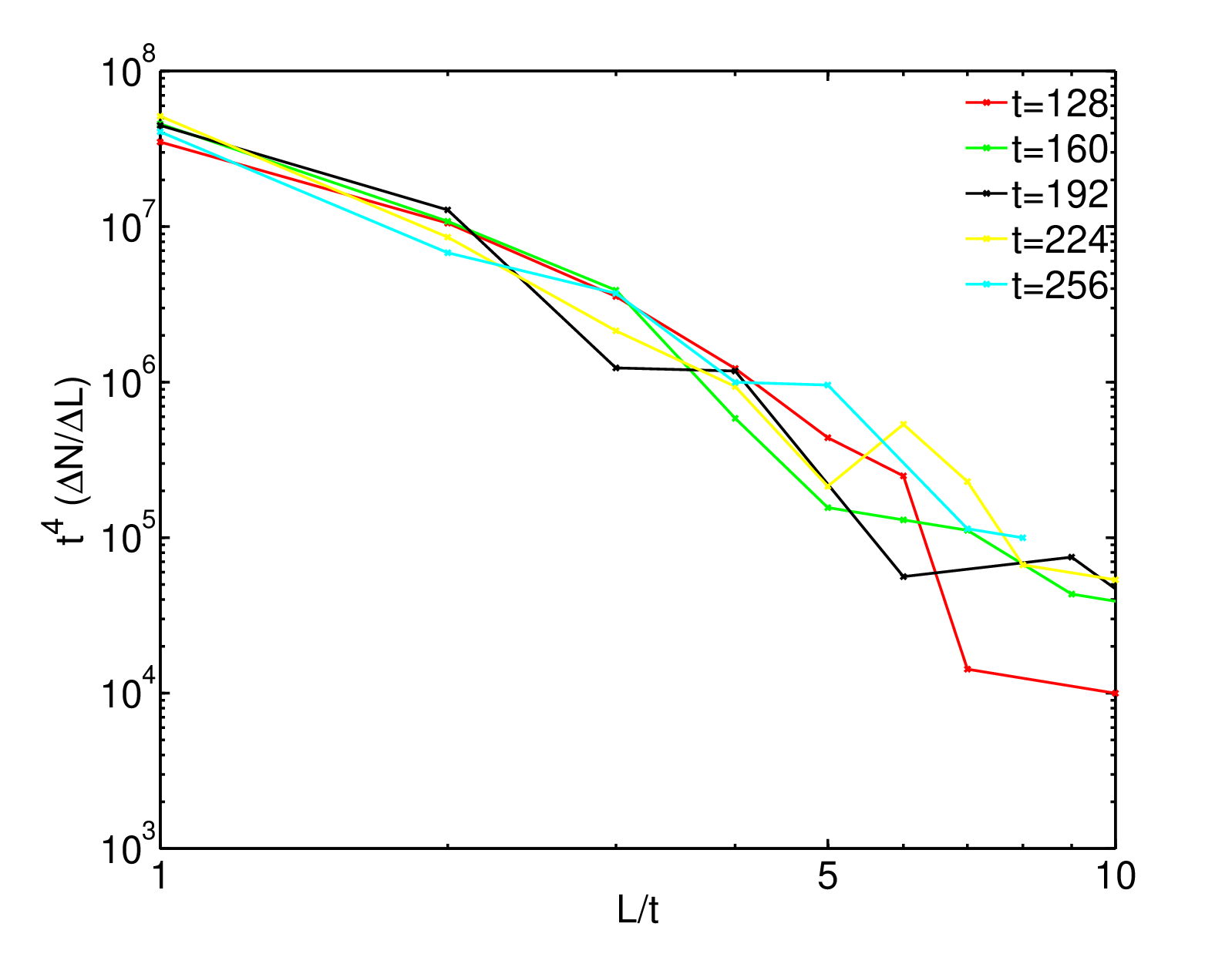
The length distribution of independent loops is plotted in Fig. 12, averaged over 20 simulations in radiation era. The figure uses logarithmic binning and shows the distribution of loops at four different times. We see that some of the loops are fairly large, with length much greater than the inter-string separation . Such loops should arguably be regarded as part of the infinite network. Indeed, if the diameter of a loop is larger than a few times (or ) for a given time, the loop is very likely to reconnect to the network. If we exclude loops longer than (), the percentage of string length in loops drops to (). These values are in agreement with previous field theoretical simulations where a loops were found to account for a few percent of the total string length Vincent.
Simulation movies show that loops that decouple from the network do not oscillate as they would in Nambu-Goto simulations, but rather shrink and disintegrate. This could be expected, since it is well known that in order to observe oscillating loops in field theory simulations one would need very large loops and very small values of the lattice spacing. Additional damping, through particle emission from loops, may be due to the presence of short-wavelength string excitations in the initial conditions, as indicated by the numerical results of Refs. Moore98; Olum00. The short lifetimes of the loops in our simulations explain, at least in part, the relatively small amount of string in loops, as compared to the Nambu-Goto simulations.
In any case, we checked the loop distribution in our simulations for scaling behavior. On dimensional grounds, the number density of loops per unit length interval in a scaling network should have the form
| (34) |
Defining as the number of loops between sizes and and , we plot in Fig. 12 the (binned) quantity , obtained for 5 different times and averaged over 20 simulations. In a situation where the loop distribution scales, all the lines should line on top of one another. We see that the graph in Fig. 12 does indeed exhibit scaling.
III.6 Effect of higher binding energy
We ran some simulations with a greater value of the string binding parameter, , in order to try to understand how sensitive our results were to the precise value of . The main difference encountered in these simulations was the fraction of bound string increased by a factor (see Fig. 13). Our analysis showed that the effect on the correlation lengths and on the loop distribution was very small. Actually, the values of the coefficient of the different length measures where the same as in the case, the only difference being a smaller for this case ( for flat, radiation and matter eras, respectively).

IV Conclusions and discussion
We performed numerical simulations of the formation and evolution of string networks using the Saffin’s model for interacting strings. The model has two types of Abelian gauge strings, and , with an attractive interaction which gives rise to bound -strings. Starting with a randomized high-energy field distribution, we found that an interconnected string network is indeed formed, consisting of and strings, as well as their bound states, joined together at -type junctions. No higher -strings were observed in the simulations.
Throughout each simulation, the network is dominated by a single (“infinite”) net, with occasional small nets and a fair number of disconnected closed loops being formed in the course of the evolution. The characteristic length scale of the network approaches the scaling regime where it grows proportionally to time, with , in both radiation and matter eras, as well as in flat spacetime. Other characteristic length scales, such as the length of segments, the typical correlation length of and strings or the typical distance between junctions also scale.
A surprising feature of our simulation is that bound -strings constitute only a small fraction of the total string length (). Also, the average length of -segments is much shorter than the length of - or -string segments. This is in contrast with analytic models Tye05; Shellard07 predicting all lengths to be fairly equal. From movies of the simulations one can see that -segments do not always form when an -string meets a -string (even for relatively high bounding energies); on the contrary, the formation of bound segments is rather infrequent. Even though new -segments are constantly formed, their lifetime is relatively short, usually less than the Hubble time, as the segments are “unzipped” by the free and ends pull them in different directions.
Even though, with our general initial condition configuration, most of the typical distances in the network showed a scaling behaviour, the average comoving lengths of and segments did not. These lengths remained much larger than the typical correlation length throughout the simulation. This evolution regime cannot continue indefinitely, since the correlation length would eventually catch up with the segment lengths and . In an attempt to go beyond this transient regime and reach true scaling, we introduced an extra period of strong damping at early times (which has the effect of decreasing ) and pushed the parameters to extend the dynamic range of the simulation. We found that the system does seem to approach a regime where all characteristic lengths scale linearly with time. If this were the true scaling regime, it would provide us, among other things, with the means to calculate CMB power spectra predictions from the field theoretical model as in BHKU06; Bevis:2007gh; Bevis:2007qz; Urrestilla:2007sf. But due to a relatively short duration of the linear evolution and to likely presence of spurious damping, our simulations cannot be relied upon for a quantitatively accurate description of scaling.
Disconnected closed loops constitute about of the total string length. Some of these loops are very large and will very likely reconnect into the main network again. If one factors out disconnected loops of length larger than a few times the correlation length, the total string length in loops drops to below , in agreement with Vincent. We examined the length distribution of loops in the network and found that, even though out parameter choice is not expected to resolve accurately string dynamics, these distributions seem to scale.
The network properties in our simulations are closer to those of superstring networks than they were in earlier simulations that used -strings or non-linear sigma-models. However, there is still an important differences. On the one hand, our and strings have the same tension, as opposed to and strings. On the other, collision of same-type strings in our model always result in reconnection (unless the string segments are moving extremely fast AP06), while in the case of superstrings the reconnection probability is and can even be small Tye03; DV04; JJP05. This feature can be accounted for in Nambu-Goto and analytic models.
The efficiency of various energy loss mechanisms by the string network remains a topic for future research. Energy loss to loop production appears to be substantial, considering that the length in loops at any time is a few percent of the total and that the loops do not stay around for long and rapidly decay. Another important energy loss mechanism in field theory simulations is direct particle emission from strings Vincent; BH07. In fact, the analysis in Shellard07 shows that emission of particles and of tiny loops which immediately decay into particles is the dominant energy loss mechanism for a single string network, so it probably dominates in our simulations as well. It has been argued in Moore98; Olum00; Shellard07 that this effect is spurious and is due partly to insufficient resolution of the simulations and partly to excessive amount of noise in the initial conditions. This issue is not completely settled, since some of the recent Nambu-Goto simulations Sakellariadou07 and analytic treatments Polchinski07 indicate continuous production of microscopic loops throughout the network evolution.
In summary, what have we learnt from our simulations? We have demonstrated that an interconnected network of strings can indeed form at a symmetry breaking phase transition. This network shows no tendency to freeze to a static configuration. On the contrary, it appears to approach scaling, with all characteristic lengths growing linearly with time. Qualitatively, our results indicate that bound strings constitute only a small part of the total string length and that the and string segments are rather wiggly, having lengths significantly greater than the correlation length . The latter property leads to relatively frequent self-intersections and allows the network to lose a substantial fraction of its energy in the form of closed loops. Our simulations also indicate that the true scaling evolution may be preceded by a transient regime in which the comoving lengths of and -segments remain nearly constant in time.
Some of the shortcomings of our approach can be overcome in Nambu-Goto-type simulations (e.g., of the kind developed in Siemens01) or in analytic models (along the lines of Tye05; Shellard07). Either of these approaches, however, requires some microphysical input. For example, one needs to know under what conditions a bound string is formed in a string collision, what fraction of the binding energy of the newly formed string is radiated away, etc. The advantage of a direct field theory simulation is that it accurately represents the microphysics. A combination of all three approaches will probably be needed to reach a full understanding of network evolution.
V Acknowledgements
We would like to thank José Juan Blanco-Pillado, Mark Hindmarsh, Andrew R. Liddle, Ken Olum and Vitaly Vanchurin for useful discussions. This work was supported by the US National Science Foundation (JU and AV), by Marie Curie Intra-European Fellowship MFIT-CT-2005-009628 and FPA2005-04823 (JU). This work has also been supported by the Spanish Consolider-Ingenio 2010 Programme CPAN (CSD2007-00042).The simulations were performed on cosmos, the UK National Cosmology Supercomputer, supported by SGI, Intel, HEFCE and PPARC.
References
- (1) For recent reviews, see J. Polchinski, Introduction to cosmic - and -strings, arXiv:hep-th/0412244; A.C. Davis and T.W.B. Kibble, Contemp. Phys. 46, 313 (2005).
- (2) M. Majumdar and A. Christine-Davis, JHEP 0203, 056 (2002).
- (3) S. Sarangi and S.H. Tye, Phys. Lett. B536, 185 (2002).
- (4) N.T. Jones, H. Stoica and S.H. Tye, Phys. Lett. B563, 6 (2003).
- (5) G. Dvali and A. Vilenkin, JCAP 0403, 010 (2004).
- (6) E.J. Copeland, R.C. Myers and J. Polchinski, JHEP 0406, 013 (2004).
- (7) P.M. Saffin, JHEP 09, 011 (2005).
- (8) M. Donaire and A. Rajantie, Phys. Rev. D73, 063517 (2006).
- (9) Y. Cui, S.P. Martin, D.E. Morrissey and J.D. Wells, arXiv:0709.0950 [hep-ph].
- (10) M. Aryal, A.E. Everett, A. Vilenkin and T. Vachaspati, Phys. Rev. D34, 434 (1986).
- (11) T.W.B. Kibble, J. Phys. A9, 1387 (1976).
- (12) P. McGraw, Phys. Rev. D57, 3317 (1998).
- (13) A. Vilenkin, Phys. Rev. Lett. 53, 1016 (1984).
- (14) M. Bucher and D.N. Spergel, Phys. Rev. D60, 043505 (1999).
- (15) T. Vachaspati and A .Vilenkin, Phys. Rev D35, 1131 (1987).
- (16) E.J. Copeland and P.M. Saffin, JHEP 0511, 023 (2005).
- (17) S.-H. Tye, I. Wasserman and M. Wyman, Phys. Rev. D71, 103508 (2005).
- (18) A. Avgoustidis and E.P.S. Shellard, arXiv: astro-ph/0705.3395.
- (19) C.J.A.P. Martins, Phys. Rev. D70, 107302 (2004).
- (20) D. Spergel and U.-L. Pen, Ap.J. 491, L67 (1997).
- (21) M. Hindmarsh and P.M. Saffin, JHEP 0686, 066 (2006).
- (22) H. Firouzjahi, arXiv:hep-th/0710.4609.
- (23) A. Rajantie, M. Sakellariadou and H. Stoica, arXiv:0706.3662 [hep-th]
- (24) E.R. Bezerra de Mello, Y. Brihaye and B. Hartmann, Phys. Rev. D67, 045015 (2003)
- (25) A. Achúcarro and J. Urrestilla, Phys. Rev. D68, 088701 (2003)
- (26) E.R. Bezerra de Mello, Phys. Rev. D68, 088702 (2003)
- (27) A. Achúcarro, B. Hartmann and J. Urrestilla, JHEP 0507, 006 (2005)
- (28) W.H. Press, B.S. Ryden and D.N. Spergel, Ap. J. 347, 590 (1989)
- (29) B.S. Ryden, W.H. Press and D.N. Spergel, Ap. J. 357, 293 (1990)
- (30) J.N. Moore, E.P.S. Shellard and C.J.A.P. Martins, Phys. Rev. D65, 023503 (2001).
- (31) N. Bevis, M. Hindmarsh, M. Kunz and J. Urrestilla, Phys. Rev. D75, 065015 (2007)
- (32) K.J.M. Moriarty, E. Myers and C. Rebbi, Phys. Lett. B207, 411 (1998)
- (33) UK National Cosmology Supercomputer: SGI Altix 3700 containing 152 1.3 GHz Intel Itanium II CPUs, www.damtp.cam.ac.uk/cosmos/
- (34) J. Urrestilla, A. Achúcarro, J. Borrill, A.R. Liddle, JHEP 0208, 033 (2002)
- (35) M. Pickles and J. Urrestilla, JHEP 0301, 052 (2003);
- (36) A. Achúcarro, P. Salmi and J. Urrestilla, Phys. Rev. D75, 121703 (2007)
- (37) J.J. Blanco-Pillado and K.D. Olum, private communication.
- (38) E.J. Copeland, T.W.B. Kibble, D.A. Steer, Phys. Rev. Lett. 97, 021602 (2006)
- (39) E.J. Copeland, H. Firouzjahi, T.W.B. Kibble and D.A. Steer, arXiv:0712.0808 [hep-th].
- (40) G. Vincent, N. D. Antunes, M. Hindmarsh, Phys. Rev. Lett. 80, 2277 (1998)
- (41) V. Vanchurin, K.D. Olum and A. Vilenkin, Phys. Rev. D74, 063527 (2006).
- (42) C.J.A.P. Martins and E.P.S. Shellard, Phys. Rev. D73, 043515 (2006).
- (43) C. Ringeval, M. Sakellariadou and F. Bouchet, JCAP 0702, 023 (2007).
- (44) K.D. Olum and V. Vanchurin, Phys. Rev. D75, 063521 (2007).
- (45) J.N. Moore and E.P.S. Shellard, arXiv:hep-ph/9808336.
- (46) K.D. Olum and J.J. Blanco-Pillado, Phys. Rev. Lett. 84, 4288 (2000).
- (47) N. Bevis, M. Hindmarsh, M. Kunz and J. Urrestilla, arXiv:astro-ph/0702223.
- (48) N. Bevis, M. Hindmarsh, M. Kunz and J. Urrestilla, Phys. Rev. D76, 043005 (2007)
- (49) J. Urrestilla, N. Bevis, M. Hindmarsh, M. Kunz and A.R. Liddle, arXiv:0711.1842 [astro-ph].
- (50) A. Achucarro and R. de Putter, Phys. Rev. D74, 121701 (2006).
- (51) M.G. Jackson, N.T. Jones and J. Polchinski, JHEP 10, 013 (2005).
- (52) S. Borsanyi and M. Hindmarsh, arXiv:0712.0300 [hep-ph].
- (53) F. Dubath, J. Polchinski and J.V. Rocha, arXiv:astro-ph/0711.0994.
- (54) X. Siemens, X. Martin and K.D. Olum, Nucl. Phys. B595, 402 (2001).