BNL-HET-07/11, CU-TP-1180, Edinburgh 2007/12, KANAZAWA-07-10, RBRC-681, SHEP-07-20
Non-perturbative Renormalization of Quark Bilinear Operators and using Domain Wall Fermions
Abstract
We present a calculation of the renormalization coefficients of the quark bilinear operators and the mixing parameter . The coefficients relating the bare lattice operators to those in the RI/MOM scheme are computed non-perturbatively and then matched perturbatively to the scheme. The coefficients are calculated on the RBC/UKQCD 2+1 flavor dynamical lattice configurations. Specifically we use a lattice volume, the Iwasaki gauge action at and domain wall fermions with .
pacs
11.15.Ha, 11.30.Rd, 12.38.-t 12.38.GcI Introduction
The RBC and UKQCD collaborations have recently performed the first simulations with 2+1 flavor domain wall fermions Antonio et al. 2007a; Allton et al. 2007; Boyle 2007. Much interesting phenomenology requires the conversion of bare lattice quantities to a less arbitrary and more perturbatively amenable continuum scheme. In particular, this is true for the determination of weak matrix elements such as and for the Standard Model parameters such as quark masses. Of course, physical quantities are independent of the choice of renormalization procedure, nevertheless theoretical predictions are often given in terms of the parameters of the theory ( and quark masses) which require renormalization. In addition, for many processes (e.g. mixing) the amplitudes are factorized into products of perturbative Wilson coefficient functions and operator matrix elements which contain the long-distance effects. The Wilson coefficients and operator matrix elements need to be combined with both evaluated in the same renormalization scheme. The purpose of this paper is to determine the factors by which matrix elements computed in our numerical simulations should be multiplied in order to obtain those in the scheme which is conventionally used for the evaluation of the coefficient functions.
In principle, for a sufficiently small lattice spacing and a sufficiently large renormalization scale , it is possible to perform the renormalization of the bare lattice operators using perturbation theory. However, in practice the coefficients of lattice perturbation theory are frequently large leading to a poor convergence of the series and even with attempts such as tadpole improvement to resum some of the large contributions, it appears that the typical -loop correction is numerically of , in contrast to continuum perturbation theory where the corresponding contributions are of . A related difficulty is the choice of the best expansion parameter (), for example between some tadpole improved lattice coupling or the coupling. In practice, at one-loop order, different reasonable choices can lead to significantly different results. For the quark bilinear operators and considered in this paper, we present the perturbative results and illustrate these points in Section II.
The main purpose of this paper is to avoid the uncertainties present when using lattice perturbation theory by implementing the Rome-Southampton RI/MOM non-perturbative renormalization technique Martinelli et al. 1995. The key idea of this technique is to define a sufficiently simple renormalization condition such that it can be easily imposed on correlation functions in any lattice formulation of QCD, or indeed in any regularization - that is, the condition is regularization invariant (RI). We therefore introduce counter-terms for any regularization such that a Landau gauge renormalized n-point correlation function with standard MOM kinematics at some scale has its tree level value. This condition is simple to impose whenever the renormalized correlation function is known in any regularization. It applies equally well to both perturbative expansions to any order and to non-perturbative schemes such as the lattice, and thus RI/MOM is a very useful interface for changing schemes. In particular, only continuum perturbation theory and the lattice regularization are required to obtain physical results from a lattice calculation.
Our choice of lattice action is important for the efficacy of the RI/MOM technique. With domain-wall fermions, errors and chiral symmetry violation can be made arbitrarily small at fixed lattice spacing by increasing the size of the fifth dimension. This allows us to avoid the mixing between operators which transform under different representations of the chiral-symmetry group; this is a very significant simplification compared to some other formulations of lattice QCD. The action and operators are also automatically improved.
Another important property of DWF is the existence of (non-local) conserved vector and axial currents. This will be discussed in detail below.
In this paper we study the renormalization of the quark bilinear operators , where is one of the 16 Dirac matrices, and of the four-quark operator . Table 1 contains a summary of our results, relating bare operators in the lattice theory with Domain Wall Fermions and the Iwasaki gauge action at (GeV, see Section III for further details) to those in two continuum renormalization schemes. Columns three through five give the three independent Z factors which, when multiplying the appropriate bilinear lattice operator, convert that operator into one normalized according to either the RI/MOM or (NDR) schemes. The final column contains the combination of factors needed to convert a lattice result for the parameter into the corresponding RI/MOM or (NDR) value.
The plan of the remainder of the paper is as follows. In the following section (Section II) we start by reviewing the perturbative evaluation of the renormalization constants; the results can later be compared with those obtained using the non-perturbative procedures. In Section III, we begin the description of the non-perturbative computations with a brief introduction to the details of our simulation and to the computation of the quark propagators which are the basic building blocks for all our subsequent calculations. In Section IV we give a short introduction to the regularization independent (RI/MOM) scheme. In this section we also discuss the renormalization of flavor non-singlet bilinear operators, including the check of the Ward-Takahashi identities. The discussion of the renormalization of the four-quark operators and the results for the renormalization constant for are presented in Section V. Section VI contains a brief summary and our conclusions.
II Perturbation Theory
Before proceeding to describe our non-perturbative evaluation of the renormalization constants we briefly review the corresponding (mean field improved) perturbative calculations. Specifically, we present perturbative estimates for the renormalization constants of the quark bilinears and . These can then be compared to those obtained non-perturbatively below. The ingredients for the perturbative calculations and a detailed description of the procedure can be found in refs. Aoki et al. 2003; Aoki and Kuramashi 2003.
Writing the domain wall height as , the bare value of in our simulation is . The mean field improved value of is then given by
| (1) |
where the link variable is defined by and is the value of the plaquette in the chiral limit.
We define the renormalization constant, , which relates the bare lattice operator, , to the corresponding renormalized one in the scheme at a renormalization scale of by:
| (2) |
Here for the scalar and pseudoscalar densities, vector and axial-vector currents and tensor bilinear and for the operator which enters into the - mixing amplitude (or more precisely for the ratio of the operator and the square of the local axial current, which is the relevant combination for the determination of ). The one-loop, mean field improved estimates for the are:
| (3) | |||||
| (4) | |||||
| (5) | |||||
| (6) |
where is the second Casimir invariant for the gauge group . Here is the quantum correction to the normalization factor of the physical quark fields (the factors depending on this normalization cancel in the evaluation of ). At one-loop order in perturbation theory
| (7) |
In obtaining the coefficients in Eqs. (3) – (7) we have interpolated linearly between the entries for and in tables III and IV of ref. Aoki et al. 2003 to the mean-field value of . Since the mean-field value of is so close to the quoted values at , we prefer this procedure to using the general interpolation formula quoted in Aoki et al. 2003. The difference between the two procedure is negligible compared to the remaining systematic uncertainties.
In order to estimate the numerical values of the renormalization constants we have to make a choice for the expansion parameter, i.e. the coupling constant . Here we consider two of the possible choices, the mean-field value as defined in eq.(62) of ref. Aoki and Kuramashi 2003 and the coupling, both defined at . The mean field improved coupling constant is given by
| (8) |
where is the bare lattice coupling constant (), and the remaining parameters are defined in ref. Aoki and Kuramashi 2003 and take the numerical values , and for , . We therefore obtain
| (9) |
Such a value of the coupling is significantly lower than that in the scheme at the same scale, for which we take, .
The difference in the two values of the coupling constant leads to a significant uncertainty in the estimates of the renormalization constants at this order, as can be seen in Table 2. The need to eliminate this large uncertainty is the principle motivation for the use of non-perturbative renormalization. The entries in Table 2 are the factors by which the matrix elements of the bare lattice operators should be multiplied in order to obtain those in the (NDR) scheme at the renormalization scale GeV.
Finally we perform the renormalization group running from GeV to obtain the normalization constants at other scales, and in particular at the conventional reference scale of GeV (see Table 3). In each case we use the highest order available for the anomalous dimension; two loops for , three loops for the tensor operator and four loop for the scalar/pseudoscalar densities. This is the same procedure which we use for the non-perturbatively renormalized normalization constants below and the details and references to the anomalous dimensions are presented in sections IV.6, IV.7 and V.4 below. The numbers in Table 3 are the factors by which the matrix elements of the bare lattice operators should be multiplied in order to obtain those in the (NDR) scheme at GeV. The entries in the first column indicate which coupling was used in matching between the bare lattice operators and the (NDR) scheme at GeV, i.e. before the running to other scales.
III Simulation Details
The calculations described below were performed on the 2+1 flavor dynamical lattice configurations generated by the RBC and UKQCD collaborations Allton et al. 2007. The lattices were generated with the Iwasaki gauge action at and the domain-wall fermion action with . The size of the lattices used in this work is . The lattice spacing is GeV and the residual mass in lattice units Lin and Scholz 2007. We have 3 independent ensembles with light sea quark mass 0.01, 0.02 and 0.03 respectively. The strange sea quark mass is fixed at 0.04. For each ensemble, we have used 75 configurations, starting from trajectory number 1000 and with trajectory separation 40.
Following the Rome-Southampton RI/MOM non-perturbative renormalization procedureMartinelli et al. 1995; Blum et al. 2002, the lattices are first fixed in Landau gauge. Then, on each gauge-fixed configuration, we measure the point-point quark propagators with periodic boundary conditions in space and time, where is the source position and is the sink. We have chosen four different sources to generate the propagators,
| (10) |
Next, a discrete Fourier transform is performed on the propagators,
| (11) |
where
| (12) |
is a four-vector of integers and
| (13) |
For the we take values in the ranges
| (14) |
and require that the squared amplitude of the lattice momenta is in the range . In this paper, for simplicity of notation we frequently use lattice units for dimensionful quantities such as and . When we particularly wish to emphasize the nature of the discretization errors we explicitly reinstate the lattice spacing, writing for example, or .
IV Renormalization of Quark Bilinears
We now discuss how Green functions computed on the lattice can be used to obtain the non-perturbative renormalization constants relating bilinear operators defined on the lattice to those normalized first according to the RI/MOM and then the scheme. In the first two subsections below, Sections IV.1 and IV.2 we briefly introduce the definitions and notation that we use in the rest of this paper. Some of these are extracted from the earlier RBC paper on quenched lattices Blum et al. 2002 and are included here for completeness.
The definition of renormalization factors and for the quark wave function and mass in the RI/MOM scheme are given in Section IV.1. The basic amputated quark-bilinear vertex functions are defined in Section IV.2 and the conditions defining the RI/MOM scheme are written down. Since our calculations are necessarily performed at finite momenta, the effects of chiral symmetry breaking coming from both the non-zero quark masses and spontaneous chiral symmetry breaking are visible. We discuss these effects in detail in Section IV.3 for the important case of the vector and axial vector vertex functions.
Next, as a consistency check for our methods, we discuss the accuracy with which our off-shell vertex amplitudes satisfy the axial and vector Ward-Takahashi identities in Sections IV.4 and IV.5 respectively. In the later section, the determination of is also discussed. In Section IV.7 we compare the observed scale dependence of with that predicted by perturbation theory and interpret the differences as coming from errors. These are removed to determine first and then . A similar determination of and then is presented in Section IV.7. Finally, in Section IV.8, results for the tensor vertex renormalization factor are obtained.
IV.1 Quark mass and wavefunction renormalization
First, we define the renormalization coefficients for the quark field and the quark mass as the ratio between the renormalized quantities and their bare counterparts,
| (15) | ||||
| (16) |
where and are the renormalized and the bare quark wavefunction, and and are the renormalized and the bare quark mass. With domain-wall fermions,
| (17) |
where is the input quark mass and is the residual mass. The renormalized propagator (in momentum space) is
| (18) |
where is the momentum of the quark propagator.
Since domain wall quarks enter the calculations described here in three different ways we must be careful to clearly distinguish their three distinct masses. As described above, our calculations are performed with 2+1 flavors of dynamical quarks. We will use the variable to label the input mass for the light dynamical quarks and for that of the dynamical strange quark. Since we often evaluate products of propagators which depend on a third quark mass, that mass is labeled . In some cases the limit may be an adequate definition of the chiral limit. However, in order to deal with simple results from which a weak quark mass dependence has been removed we will often consider the “unitary” case and take the limit . Of course, in this case remains non-zero but since its value is never changed this causes no immediate confusion. Underlying the validity of the Rome-Southampton renormalization scheme is the use of infrared-regular renormalization kinematics. Therefore, as our renormalization scale becomes larger and future calculations more accurate, even this weak quark mass dependence will completely disappear.
As discussed in detail in Blum et al. 2002, the renormalization technique requires the existence of a window of momenta such that
| (19) |
In practice, however, violation of these restrictions, especially at the higher boundary, has to be considered. Due to the spontaneous breaking of the chiral symmetry as illustrated by the non-trivial difference between and at low momenta (see section IV C) we have to rely on the calculation in the relatively high momentum region, where . Fortunately, the effects from breaking the restriction imposed by the finite lattice spacing are small and predictable. They introduce an error of to the renormalization coefficients which can be removed by quadratic fitting to the momentum dependence. A more detailed investigation of this issue is presented in Blum et al. 2002.
It is possible in principle to relax the constraint in eq.(19) by performing step scaling, i.e. by matching the renormalization conditions successively to finer (and also smaller in physical units) lattices. This is beyond the scope of this paper.
The regularization independent (RI/MOM) scheme is defined such that by adjusting the renormalization coefficients and at the renormalization scale , and restricting in a suitable window, we have:
| (20) | ||||
| (21) |
Imposing these conditions on the lattice and taking into account the dynamical breaking of chiral symmetry at low energies, the additive mass renormalization and lattice artifacts, we have the following asymptotic behavior Blum et al. 2002 for relatively large :
| (22) |
The left-hand-side of Eq.(22) at each of the unitary points () is calculated as the inverse of the average over all propagators, where the average is performed over all sources and configurations:
| (23) |
where and labels each configuration. (For brevity, in this equation and in the following we will suppress the subscript “latt”on all the lattice propagators. In the following text, unless otherwise specified, all the propagators without a subscript denote the lattice propagators.) Because of possible correlations between propagators with different sources calculated on the same configuration, each group of 4 propagators from the same configuration is considered as one jackknife bin in the single-elimination procedure.
In Figure 1 we plot the results for as a function of the momentum and tabulate the corresponding numerical values in Table 4. In addition to our results for non-zero quark mass, we also plot and tabulate the results extrapolated to the chiral limit where for each momentum. Two quantities of interest can be deduced from the mass dependence shown in Figure 1. First, the chiral limit gives a measure of the spontaneous and explicit chiral symmetry breaking and is given in the left-most column of Table 4. Second determining the slope with respect to provides one method to calculate . This is used later in Section IV.5 to test the vector Ward Identity which relates this to a second method of computing .
IV.2 Renormalization of flavor non-singlet fermion bilinears
We now consider the renormalization of quark bilinear operators of the form , where is one of the 16 Dirac matrices. The corresponding renormalization constant is the factor relating the renormalized and bare bilinear operators:
| (24) |
where is the renormalization scale and we will treat only local operators where the lattice fields and in the bilinear operator are evaluated at the same space-time point.
Following the Rome-Southampton prescriptionMartinelli et al. 1995 for renormalization in the RI/MOM scheme, we define the bare Green functions between off-shell quark lines, and evaluate their momentum-space counterparts on the lattice, averaged over all sources and gauge configurations,
| (25) |
We then amputate this Green function using the averaged propagators,
| (26) |
where is calculated according to Eq. (23). The bare vertex amplitudes are obtained from the amputated Green functions as follows Martinelli et al. 1995; Blum et al. 2002:
| (27) | ||||
| (28) | ||||
| (29) | ||||
| (30) | ||||
| (31) |
The values of all the five bare vertex amplitudes at the unitary mass points are presented in Table 5 through Table 7. Finally, by requiring that the renormalized vertex amplitudes satisfy
| (32) |
we can calculate the relevant renormalization constants.
Equations (24) through Eq. (32) describe the schematic procedure used to calculate the renormalization coefficients of quark bilinears. In practice however, with finite quark masses and a limited range of momenta, we have to consider lattice artefacts and other systematic uncertainties. We explain the details in the following sections.
IV.3 Chiral symmetry breaking and
In this section we examine the effects of both the low-energy spontaneous chiral symmetry breaking present in QCD and our non-zero quark masses on the large-momentum, off-shell propagators which we are using to impose non-perturbative renormalization conditions. A good quantity to study in order to understand these effects is the difference of the off-shell vector and axial vector vertex functions.
IV.3.1 Numerical results for
In the limit of a small mass and a large momentum, we expect
| (33) |
or equivalently,
| (34) |
for .
However, with finite quark masses and at relatively low momenta and may receive different contributions of the form
| (35) |
and
| (36) |
Here we are exploiting the chiral symmetry of large domain wall fermions which implies that a difference between and requires the mixing of and representations and hence involves a product of two quantities which transform as and . This requires the two powers of in Eq. (35) and the product in Eq. (36). The extra factors of and come from naive dimensional analysis.
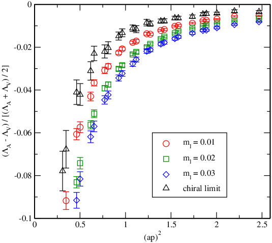
To determine how much chiral symmetry breaking is present in our calculation, we examine the relative difference between and . In Figure 2 we plot the quantity as a function of momentum. At relative low momenta, , we observe that this quantity is quite large . Furthermore, even when we extrapolate to the chiral limit, where the terms in Eqs. (35) and (36) both vanish, the difference between and does not vanish. Here to obtain the chiral limit shown in Figure 2 we perform a linear extrapolation . While a quadratic extrapolation gives a similar result, this linear choice is motivated by the analysis presented in Section IV.3.3.
Since the explicit chiral symmetry breaking effects needed to split and can be argued Christ 2006 to be , we would not expect this difference to reflect explicit, finite-, domain wall chiral symmetry breaking. In fact, similar deviations between and are seen on lattice ensembles without fermion loops where explicit domain wall chiral symmetry breaking is expected to be smaller. This is shown in Figure 3 where we plot the same quantities from a quenched simulation using the DBW2 gauge action. Thus, it appears that this difference represents the high energy tail of QCD dynamical chiral symmetry breaking rather than the explicit chiral symmetry breaking coming from the finite value of .
While the effects of spontaneous chiral symmetry breaking will not vanish in the limit , it is unlikely that the substantial difference found for in the chiral limit can be explained by a dimension-6 condensate such as
| (37) |
since it is suppressed by six powers of momentum and appears to be too small for the size of the breaking we have observed. We have also fit the quantity to different powers of , as is shown in Figure 4, and it is clear that the momentum dependence of the chiral symmetry breaking term is dominated by or , very different from that naive dimensional analysis suggests should appear in the term above.
IV.3.2 Effects of exceptional momenta
In fact, we believe that the origin of the difference between and is different. Our choice of kinematics corresponds to so called “exceptional momenta”, i.e. a momentum transfer is zero. This invalidates the naive power counting estimates used above and permits the low-energy, spontaneous chiral symmetry breaking to split and with only a suppression for large , as we now explain. Begin by considering a general, amputated Feynman graph with external fermion lines and external boson lines. Recall that for connected graphs the degree of divergence of is defined as . If the graph is disconnected then its degree of divergence is the sum of those of its connected components. Now imagine that each external line of carries an incoming momentum for , where is an over-all scale factor. The asymptotic behavior for large of the amplitude corresponding to such a graph will be where is the degree of divergence of a subgraph . This subgraph must be chosen so that i) there exists a routing of the internal momenta within such that all lines carrying momenta proportional to lie within and ii) possesses the least negative degree of divergence of all those subgraphs satisfying i) Weinberg 1960; Itzykson and Zuber 1980. Note, that may equal the original graph and may itself be disconnected.
The most familiar situation is the case of non-exceptional momenta, defined as a momentum configuration in which no proper partial sum of the external momenta vanishes. Under these circumstances all subgraphs obeying i) must be connected. (Otherwise there would be zero momentum transfer between the groups of momenta entering each of the disconnected components.) This implies that the subgraph with the least negative degree of divergence is one with no additional external lines beyond those already appearing in which in turn implies that this subgraph is the entire graph . For the case of the vertex graph of interest, we deduce a constant behavior (up to logarithms) since . (Here it is convenient to view this vertex graph as resulting from a normal Feynman graph in which an external vector boson is coupled to the vertex so the rules discussed above directly apply.)
This analysis not only gives the leading asymptotic behavior but also insures that extracting a few extra factors of the mass or the chiral condensate will make the degree of divergence of that graph more negative and hence make its asymptotic fall-off more rapid, in the fashion suggested by naive power counting. For the case of interest, we would like to restrict a subset of the internal fermion lines of our graph to carry only low momenta so that they will reflect the low-energy, spontaneous chiral symmetry breaking of QCD. By definition, these low momentum lines cannot enter the subgraph discussed above whose degree of divergence determines the asymptotic behavior of amplitude being studied. In order to split and , chiral symmetry breaking transforming as an (8,8) under is required. This in turn requires that this low energy, excluded subgraph must be joined to the remainder of the graph by at least four fermion lines.
Such a circumstance is illustrated by the general vertex graph in Figure 5, contained in the outer dashed box. Here we have identified a subgraph which carries only low momenta and can therefore transform as (8,8) even in the limit of vanishing quark mass, . For the case of non-exceptional momenta, we must apply Weinberg’s theorem to the subgraph , enclosed in the inner dashed box, through which, by assumption, all of the large momenta entering the vertex and the two external fermion lines must be routed. Because of its connections to the subgraph , the subgraph has six external fermion lines and one external boson line (connected to the vertex). The resulting degree of divergence is , justifying the naive behavior in Eq. 37.
However, in our case and are being evaluated with zero momentum entering the current vertex and with a vanishing sum of the two incoming fermion momenta—a configuration of exceptional momentum. For such a choice of external momenta we can divide the subgraph identified above into two pieces and . Because the momenta are exceptional with no large momenta entering the vertex, we can route all of the large momenta through . Since has only four external fermion lines, its degree of divergence is and the behavior above has been replaced by the much less suppressed . If we think of the subgraph as a generalized chiral condensate we are seeing the asymptotic behavior
| (38) |
very consistent with our numerical results. Note the discrepancy in dimensions between Eqs. (37) and (38) will be made up by four powers of , the momentum scale to which the subgraph is restricted.
A simple class of graph allowing this behavior can be seen in Figure 6. Here the large momentum carried by the two external fermion lines can be routed through the gluon propagator that is shown explicitly so that the upper part of the diagram carries only low momenta. The large momentum behavior of the gluon propagator gives the expected behavior. The two general fermion propagators shown with the shaded “blobs” carry small momenta and, as suggested by Eq. (22), can show or chiral symmetry violation even when .
To confirm this analysis, we have also calculated the difference between and with non-exceptional momenta. We have chosen 5 different momentum scales, each corresponding to a set of momenta which satisfy the condition for five values of , as listed in Table 8 and Table 9. We then calculated and with the two external fermions carrying respectively and . The result is plotted in Figure 7, which shows that the chiral symmetry breaking vanishes almost completely with non-exceptional kinematics at medium to large momenta.
While it would be more satisfactory to perform the calculations presented in this paper using non-exceptional momenta, the resulting RI/MOM normalization conditions would not correspond to those for which perturbative matching calculations have been carried out. Thus, we would not be able to relate the quantities which we calculated to those defined in the scheme. (Of course, this difficulty will be removed when the necessary perturbative calculations have been extended to non-exceptional kinematics.) A second, less significant advantage of the exceptional momenta which we use is that the exceptional momentum conditions are satisfied by a much larger set of discrete lattice momenta permitting the RI/MOM condition to be satisfied for more fine-grained sequence of energy scales.
We now return to the calculation with exceptional momenta (), at the scale which we are most interested in, that is or , where and have a difference of about 1%. Since we have no means to determine which of these two quantities has less contamination from low energy chiral symmetry breaking we have decided to take the average as the central value for both and . The difference between or and then provides an estimate for one systematic error in our final results. The value of is plotted in Figure 8.
IV.3.3 Chiral extrapolation to vanishing quark mass
As discussed above, our use of exceptional momenta implies a suppression for both terms behaving as and . The added dimension of a term can be provided by a factor of without the need to introduce additional inverse powers of . For our largest value of , we might estimate . This suggests that we should expect a linear rather than quadratic behavior in to dominate the small quark mass limit.
The difference discussed above provides a good place to study this effect. This difference reflects the chiral symmetry breaking of interest and may make these effects stand out with possibly reduced errors because of the statistical correlations between the two quantities being subtracted. Figure 9 compares linear and quadratic fits to the dependence on the quark mass evaluated at unitary points with for GeV. In Table 10 we present the results of these two fits:
| (39) | |||||
| (40) |
for MeV. As can be seen in the Table the linear fits are favored. The linear fits have the smaller and the coefficient is significantly closer to an expected value of 1 than is the coefficient . Thus, based on both the theoretical expectation and this empirical evidence, we will adopt this linear description in the remainder of this paper and extrapolate our exceptional momentum amplitudes to the chiral limit using a linear ansatz. For the case at hand, Figure 10 shows this linear extrapolation for the average to the chiral limit for the momentum GeV. Figure 8 shows the results in the chiral limit as a function of momentum. The results in the chiral limit are also presented in Table 11.
IV.4 Axial Ward-Takahashi identity
Performing an axial rotation on the propagator leads to a relation between and , the axial Ward-Takahashi identityBlum et al. 2002:
| (41) |
In a truly chiral theory or the present DWF calculation in the limit (when chiral symmetry becomes exact and ), this identity will be obeyed configuration by configuration. However, for finite and , this relation will hold only after a gauge field average, (e.g. is only defined after such an average). Thus, we should check Eq. (41) on gauge-averaged amplitudes.
Figure 11 shows the difference between the l.h.s and r.h.s of Eq. (41), divided by their average. The case of shows relatively larger breaking of %, while the other two masses result in a smaller breaking. Since for , the term, with a value of 0.00308, represents a 30% effect, this suggests that the use of in the context of Eq. (41) may be accurate at the 25% level for this lattice spacing. Note, we expect violations coming from a dimension-five, anomalous chromo-magnetic term to be suppressed by a factor of relative to those from , making this % estimate comfortably smaller than the naive estimate of . However, the suggested growth in the size of these violations with increasing may be visible in Figure 11.
IV.5 Vector Ward-Takahashi identity and the chiral limit of
Similar to the case with , from the continuum vector Ward-Takahashi identity, we have the relation between and Blum et al. 2002:
| (42) |
We are able to check our data against this identity using the three sources, (0,0,0,0), (4,4,4,8) and (12,12,12,24) since it is only for these three sources that multiple valence mass data are available for each sea quark mass.
Figure 12 shows the difference between the two sides of Eq. (42) divided by their average. For all three sea quark masses the data agrees well with the vector Ward-Takahashi Identity (Eq. (42)) for medium to large momenta. Equation (42) implies the relation
| (43) |
and will use this equation and a calculation of to determine the mass renormalization factor in the following sections.
To extrapolate to the chiral limit, we will improve upon the discussion in Blum et al. 2002 in two regards. First, as explained above, we will exploit the asymptotic properties of Feynman amplitudes evaluated at exceptional momenta and assume that the leading mass dependence in the chiral limit will be linear in . This is different from the dependence assumed in Ref. Blum et al. 2002 where dimensional arguments, appropriate to the non-exceptional case and leading to the behavior in Eq. 35 were adopted.
Second, in contrast to that earlier quenched calculation we can examine the behavior of as a function of both the valence and light dynamical quark masses, and respectively. In Figure 13 we plot as a function of both and . The three curves are each a linear plus double pole fit to the valence quark mass dependence of the form:
| (44) |
where we have allowed the coefficients and of the constant and linear terms to vary with the dynamical light quark mass. However, we have used a common double-pole term with the behavior expected for a theory with two light flavors. Recall that this double pole term arises from topological near-zero modes Blum et al. 2002 which for two light flavors will be suppressed by two powers of the light quark mass. The data in Figure 13 shows just this behavior with the sharp turn-over at the smallest value of increasing as the light dynamical mass increases.
This double-pole can be deduced from Eq. 42. As discussed in Ref. Blum et al. 2002, the NLO, term derived from an operator product expansion of the quark propagator on the right-hand side of this equation is proportional to the chiral condensate Politzer 1976; Becirevic et al. 2000. Isolated, topological, near-zero modes of the sort that arise from a gauge field background with non-zero Pontryagin index will contribute a term to the chiral condensate which behaves as . This implies that the derivative in Eq. 42 will yield the double pole, hypothesized in Eq. 44. Such a near-zero mode will also introduce a factor of into the fermion determinant of the QCD measure for each light flavor in the theory, hence the expected factor of in the numerator of Eq. 44. In Figure 14 we show the variation of the double pole coefficient with the momentum at which the coefficient of the double pole was extracted. Also shown in this figure is a fit to the expected behavior which describes the results very well.
This understanding of the double pole terms suggests that a good strategy for extracting the chiral limit of first takes the limit of vanishing to remove this NLO double pole term and then extrapolates to . In the present case, we perform the simpler linear fit using the unitary points to obtain since we do not have the complete partially quenched results for each of our four sources.
IV.6 Mass renormalization and renormalization group running
To calculate the mass renormalization constant , as defined in Eq. (16), we can either directly take the derivative of , by following Eq. (22),
| (45) |
or we can use the Ward-Takahashi identity,
| (46) |
With the analysis described in the above sections, we find that the method with the smallest statistical uncertainty is to use as the value of . To remove the factor from (which is equal to and can be calculated as described in Section IV.2), we use the ratio calculated in Section IV.3, as well as the value obtained in Ref. Lin and Scholz 2007 using hadronic matrix elements. We therefore determine in the RI/MOM scheme by computing separately the three factors on the right-hand side of
| (47) |
Table 12 contains the values of for a variety of momentum scales.
After obtaining the lattice value of at different momenta, we divide it by the predicted renormalization group running factor to calculate the scale invariant quantity . The four-loop running formula we use is Chetyrkin and Retey 2000:
| (48) |
where is chosen such that , a value that lies within the fitting range used below. For completeness we present in the appendices the detailed procedure for running at four-loops (Appendix A) and the form of running factors (Appendix B).
As Figure 15 shows, the quantity is remarkably independent of the scale . However, in spite of the name, for other cases, the scale-invariant factors do show noticeable scale dependence and an additional correction is warranted. (See, for example, Figure 17.) We believe that the primary reason for this lack of scale invariance is the presence of lattice artifacts, namely the finite lattice spacing which introduces a small error of . Such an error can be reduced by removing the dependence in . To do this we fit this momentum dependent to the form over the momentum range and then take the limit of that fit to remove the momentum dependence. We interpret the outcome as the true . Note, we are ignoring possible dependence arising from the absence of higher order terms in the matching factor. Such scale dependence can only be removed by even higher order computation of the perturbative matching factor and such a correction is expected to be very small. While this procedure represents a negligible correction for this case of , it will have a more significant effect in the cases considered below.
Our ultimate goal is to determine which connects the bare lattice quark mass to its continuum counterpart defined according to the scheme, at the renormalization scale GeV, because the corresponding continuum renormalization is conventionally done in this scheme. So we again use Eq. (48) to calculate (2 GeV) from the scale-independent value of . Then we multiply it with the three-loop matching factor, which will also be explained in Appendix B, to match the (2 GeV) to the scheme. The final step is shown in Figure 16 and the results are given in Table 12. The renormalization constant at the desired scale is
| (49) |
The systematic error is determined by adding in quadrature our estimates of three different types of systematic error which we will now discuss.
The first is the effect on of the difference between determining from or from . This contributes an error of to . Next we must assign an error to our use of three-loop matching factor, given in Eq. (73). Here we assign an error equal to the magnitude of the final, order error in this perturbative expression, which is . While this may be a conservative estimate of the omitted terms of order and higher, it also is intended to include the errors introduced by the order estimate of the perturbative running determine the intermediate SI step used to remove the errors.
Finally we address the errors arising from our failure to extrapolate to the limit of vanishing strange quark mass. Recall, we have evaluated the chiral limit in which both the valence quark mass which enters our off-shell propagators and the dynamical light quark mass are extrapolated to zero. However, all of the gauge ensembles used in this calculation were computed with a non-zero strange quark mass . Since we are matching our Green functions to those computed in perturbation theory in the mass-independent, , limit our non-zero value for implies an additional systematic error. Because the dynamical quarks enter only through loops, their effect is different from that of the valence quarks discussed above. They do not contribute chiral symmetry breaking effects in our matrix elements. However, because of low energy chiral symmetry breaking, we do expect the dynamical quark masses to appear linearly in a quantity such as in the limit . To estimate the size of this effect, we begin with the size of the observed linear dependence, which comes from both the calculated valence and light dynamical mass dependence of . This is then multiplied by 1/2 because there is only one flavor of strange quark and by giving an error in of . The total systematic error given in Eq. 49, , is then the sum of these three errors in quadrature.
IV.7 Quark wavefunction renormalization and renormalization group running
In Section IV.3, we calculated the ratio of renormalization constants
| (50) |
To calculate , we multiply this quantity with obtained in Ref. Lin and Scholz 2007. Thus, we have evaluated the quantity in the RI/MOM scheme, which is shown in Table 13. To calculate in the scheme, we follow a similar procedure as in the previous section, and start by dividing by the perturbative running factor. As shown in Appendix C, the functional form of the running factor is quite similar to that of . The energy scale where is fixed to the value is again chosen such that .
The calculated values of vary slightly with momentum due to the presence of lattice artifacts. To remove these, we again fit the dependence to the form and extrapolate to . The procedure is shown in Figure 17. Finally, we take the scale-invariant , run up to different scales in the RI/MOM scheme, and then apply the perturbative matching factor (Appendix C) to translate it to the scheme. The values are shown in Figure 18 and Table 13. Of particular interest, the value at is
| (51) |
The systematic errors are estimated using the same procedure explained in Section IV.6. They are the sum in quadrature of the estimated errors arising from the difference (0.0061), the use of a perturbative matching factor accurate to order (0.0045) and our use of a non-zero sea quark mass (0.0035).
IV.8 Tensor Current Renormalization and Renormalization Group Running
To calculate the tensor current renormalization constant , we follow a procedure similar to those of the previous two sections. For each dynamical quark mass, we combine the ratios and in order to obtain the ratio of to in the RI/MOM scheme:
Ultimately, we use the independent hadronic matrix element calculation of , which gives , to obtain . Table 14 shows the values obtained for the in the chiral limit for a range of lattice momenta. As discussed above we have performed the chiral extrapolation using a linear functional form, and Figure 19 shows this linear extrapolation at the lattice momentum .
We obtain SI values for in the chiral limit by dividing out the tensor current perturbative running factor, the evaluation of which is described in Appendix E. Again, the SI values obtained in this way exhibit a dependence on the lattice momenta, and again we fit the momentum-dependent to the form and extrapolate to to remove the lattice artifacts, as shown in Figure 20. Finally, we run the scale-invariant back to different scales in the RI/MOM scheme and use the perturbative matching factor (Appendix E) to match to the scheme. The values are shown in Figure 21 and Table 14. At GeV, we obtain:
The systematic errors are determined in the same fashion as in the previous two sections. Specifically the errors arising from the difference (0.0054), the use of a perturbative matching factor accurate to order (0.014) and our use of a non-zero sea quark mass (0.0003) are added in quadrature.
V Renormalization Coefficients for
V.1 General procedure for computing the mixing coefficients
By the renormalization of we mean the calculation of the renormalization coefficient for the operator
| (52) |
which is the operator responsible for the mixing between and . Since for finite our theory does not posses exact chiral symmetry we must consider the possibility that this operator can mix with the four other operators with a different chiral structure:
| (53) | ||||
| (54) | ||||
| (55) | ||||
| (56) |
where they are labeled by the chirality structure of the even-parity components. The odd-parity components of these operators are not important here since they don’t contribute to mixing.
For domain-wall fermions, the mixing of with these four operators with wrong chirality should be strongly suppressed by . However, chiral perturbation theory predicts that the parameters of the operators with the wrong chirality diverge in the chiral limit Aoki et al. 2006; Becirevic 2004. To address this issue, we will describe a theoretical argument to estimate the size of the mixing terms and an actual calculation of these chirality-violating mixing coefficients on the 2+1 flavor dynamical lattices.
Following the Rome-Southampton prescription Martinelli et al. 1995; Aoki et al. 2006, we first calculate the matrix,
| (57) |
where is the amputated, four-point Green function. The Green functions are first averaged over all sources and configurations, and then amputated using the averaged propagator, in a procedure similar to the calculation of two-point amputated Green functions in Section IV.2. is a suitable projector, which projects out the component with the expected chirality (for example, the projector corresponding to is ). The subscripts .
It is straight-forward to calculate the mixing matrix at tree level which we denote as:
| (58) |
The RI/MOM renormalization condition which we adopt is then:
| (59) |
or
| (60) |
V.2 Theoretical argument for the suppression of mixing coefficients
As can be seen from the structure of the four operators in Eqs. (53), (54), (55) and (56), if they are to mix with defined in Eq. (52) then two quark fields much change chirality from left- to right-handed. For domain wall fermions such a mixing can arise from the explicit breaking of chiral symmetry coming from the finite separation between the left and right walls. The asymptotic behavior for large of the resulting mixing coefficients can be estimated using the transfer matrix for propagation in the -direction introduced by Furman and Shamir Furman and Shamir 1995. The large- limit is then controlled by matrix elements of the operator and is dominated by those four-dimensional fermion modes corresponding to eigenvalues of the transfer matrix which lie near unity.
As described in detail in Ref. Antonio et al. 2007b and in the original references cited therein, these fermion modes are believed to fall into two classes: modes localized in space-time with corresponding eigenvalues falling arbitrarily close to unity and de-localized modes characterized by a mobility edge and with eigenvalues of lying below Golterman and Shamir 2003; Golterman et al. 2005a; Golterman et al. 2005b; Svetitsky et al. 2006. Since two quarks must change chirality to produce the required operator mixing, for the case of de-localized modes such mixing will be suppressed by the two factors of needed for the propagation between the left and right walls of these two fermions, consistent with our estimate above that such effects should be of order .
However, the effects of the localized modes are more subtle. We must address the possibility raised by Golterman and Shamir Golterman and Shamir 2005 that the contribution of such a mode to is suppressed because such modes are relatively rare and the necessary coincidence with the location of the operators being mixed is unlikely. However, if present, such a mode can mix right- and left-handed fermions with little further suppression since the corresponding eigenvalue may be very close to unity. This raises the possibility that a single such mode, suppressed by a single factor of might be occupied by the two different quark flavors to provide the double chirality flip needed to mix the operators. Fortunately, as argued in Refs. Christ 2006 and Aoki et al. 2006, this is not possible because the mixing in question requires both a quark and an anti-quark or two quarks of the same flavor to propagate across the fifth dimension. This requires two distinct modes and hence incurs the double suppression which is well represented by the estimate above. Note, which will introduce errors in current calculations of Antonio et al. 2007c and will be too small to be seen in non-perturbative studies presented here.
V.3 Lattice calculation of mixing coefficients
With the procedure described in Section V.1, we can directly calculate the mixing coefficients. In particular, we have calculated the off-diagonal terms in the matrix . Figure 22 shows the mixing coefficient at different unitary masses. As in the earlier discussion of the difference, our use of exceptional external momenta permits both a linear and quadratic mass dependence. As was found in Ref. Aoki et al. 2006 and suggested by the mass dependence seen in Figure 23 a linear dependence appears reasonable and it is a linear form that we have used in determining the chiral limit shown in Figure 22.
As can be seen in Figure 22, at the chosen reference scale, or , the mixing coefficient is about and decreases when the scale is made larger. Similar to the discussion in Section IV.3, we again propose that this non-zero mixing coefficient in the chiral limit has its source in our use of exceptional momenta. Again we can determine the asymptotic behavior of the amplitude in question by determining the least negative degree of divergence of a subgraph through which all of the large external momenta can be arranged to flow. Here it is convenient to treat the operator , which is evaluated at zero momentum, as an internal vertex of dimension 6 rather than an unusual sort of external line. This alters the rules for computing the degree of divergence of a subgraph: now any connected subgraph with external fermion lines and external boson lines in which this new vertex appears, must have degree of divergence since has a dimension two higher than the usual renormalizable coupling. (As before, the degree of divergence of a disconnected graph is the sum of the degrees of divergence of its connected components.)
As in the case of the vertex amplitude discussed in Section IV.3, the appearance of exceptional momenta does not change the asymptotic behavior in the large limit with external momenta for . Even for our exceptional case , scaling with is expected. However, derivatives with respect to the quark mass or the occurrence of factors of will be strongly affected by this choice of external momenta. As is shown in Figure 24, we can identify a disconnected subgraph through which all the large external momenta can be routed which has . (Note, momentum conservation implies that if all of the large momenta can be routed within a disconnected diagram then the choice of external momenta must be exceptional.) This value implies a behavior with only low momenta flowing through the omitted subgraph . Since has four external lines it can translate standard QCD vacuum symmetry breaking into the chiral symmetry breaking that is required to produce the operator mixing shown in Figure 22.
Again, we confirm this conclusion, by recomputing the coefficient at non-exceptional momenta, as shown in Figure 25. With that choice of momenta the mixing coefficient vanishes completely within our statistical accuracy.
The other chiral symmetry breaking mixing coefficients, and are very similar to the case of just discussed. These coefficients are plotted in Figure 26 to Figure 29. Since our theoretical argument implies that the mixing coefficients are very small, i.e. and our numerical results are consistent with this implication, it is safe to neglect them and calculate the renormalization coefficient for :
| (61) |
V.4 Calculation of and renormalization group running
Using Eq. (61), the value of from Section IV.3 and the value of , we can calculate the lattice values of at different masses and momenta, as shown in Table 15. To extrapolate to the chiral limit, we again use a linear function, for the same reasons as described in Section IV.3. The linear mass fit at the scale is illustrated in Figure 30, and the value of in the chiral limit is shown in Figure 31 and Table 16.
Similar to the procedure described in Section IV.6, in order to determine from , we first divide the by the predicted running factor at one-loop order and obtain the quantity . Then we fit a quadratic function over the region to remove the dependence from induced by the lattice artifacts. Finally, we restore its perturbative running in the scheme to the scale . The perturbative running and matching factors are presented in Appendix D.
The procedure of dividing by the running and removing the dependence is shown in Figure 32, and the result of restoring the running in the scheme is shown in Figure 33. Table 16 lists at different momentum scales. The final we need in the scheme and is
| (62) |
The systematic error is calculated, following the same procedure as has been used for the previous quantities, as a sum in quadrature of the amount the result changes when is replaced by (0.0131), the size of the highest order perturbative correction being made (here of ) (0.0177) and the effect of our non-zero value for in the calculation of (0.0007).
VI Conclusions
We have presented a study of the renormalization coefficients , and on the , 2+1 flavor dynamical domain-wall fermion lattices with Iwasaki gauge action of and generated by the RBC and UKQCD collaborations. These coefficients are important components in calculations of a number of important physical quantities reported elsewhere Boyle 2007; Antonio et al. 2007c The procedure closely follows that used in an earlier study with quenched lattice configurationsBlum et al. 2002; Aoki et al. 2006. In addition to providing the Z-factors necessary to support a variety of calculations on these lattice configurations, this paper also presents a number of new results which go beyond earlier work.
First, the troublesome double pole which appears in a quenched calculation of the quantity because of topological near zero modes is now highly suppressed by the 2+1 flavor determinant. This allows us to use for an accurate calculation of . Second we have identified the large chiral symmetry breaking effects seen in the off-shell Green functions and as caused by our use of exceptional momenta. We have advanced both a theoretical discussion explaining the pattern of symmetry breaking which we have observed and a calculation with non-exceptional momenta in which these effects are dramatically reduced.
Third, for we have presented both a theoretical argument and numerical calculations showing the mixing coefficients with the operators with the wrong chirality are very small so that the calculation of can be simplified by neglecting these mixing coefficients. Finally we have exploited the earlier perturbative work of others and evaluated the factors relating the normalization of operators defined in the and RI/MOM schemes determining , , and from their non-perturbative RI/MOM counterparts to three, three, one and two loops respectively.
Acknowledgements.
We thank our collaborators in the RBC and UKQCD collaborations for assistance and useful discussions. This work was supported by DOE grant DE-FG02-92ER40699 and PPARC grants PPA/G/O/2002/00465 and PP/D000238/1. We thank the University of Edinburgh, PPARC, RIKEN, BNL and the U.S. DOE for providing the facilities on which this work was performed. A.S. was supported by the U.S. Dept. of Energy under contracts DE-AC02-98CH10886, and DE-FG02-92ER40716.Appendix A The QCD Functions and the Running of
The four-loop QCD beta functions is calculated in van Ritbergen et al. 1997 and the conventions we use are the same as in Chetyrkin and Retey 2000:
| (63) |
To calculate the coupling constant at any scales, we have used the four-loop (NNNLO) running formula for van Ritbergen et al. 1997:
| (64) |
where . (We have changed the normalization of to match the definition of the -functions coefficients.) For a numerical implementation, we start from the world-average value at Yao et al. 2006,
| (65) |
where the superscript indicates that it is in the 5-flavor region, and run across the and threshold with the matching conditions:
| (66) |
Having computed , we can calculate the coupling constant at any scale in the 3-flavor theory. For example,
| (67) |
Appendix B Perturbative Running and Matching for
In Chetyrkin and Retey 2000, the renormalization group equation for is solved to four-loop order (NNNLO) . Using the solution with our definition of the renormalization coefficients , we obtain:
| (68) |
where the function is given by:
| (69) |
with and
| (70) |
The evaluation of the coefficients of the QCD function and the running of are explained in Appendix A and the anomalous dimensions are
| (71) |
where .
When applying Eq. (68), we need to choose a value of , where the SI value is calculated. The exact value of is immaterial and for convenience we choose its value such that
| (72) |
To match the renormalization coefficients from RI/MOM scheme to scheme, we have applied the three-loop matching factor Chetyrkin and Retey 2000 obtaining:
| (73) | |||||
Appendix C Perturbative Running and Scheme Matching for
The renormalization group equation for is very similar to that for Chetyrkin and Retey 2000 and we can reuse the solution of the equation from Appendix (B) to write:
| (74) |
where the function has exactly the same functional form as defined in Eq. (69), but with the coefficients of the anomalous dimension replaced by those of :
| (75) |
The coefficients of the anomalous dimension are Chetyrkin and Retey 2000:
| (76) |
where , which represents the number of colors, and .
When we match from RI/MOM scheme to scheme, the three-loop matching factor is Chetyrkin and Retey 2000
| (77) |
Appendix D Perturbative Running and Scheme Matching for
To remove (restore) the perturbative renormalization group running of , we use the one-loop renormalization group running formula Aoki et al. 2006:
| (78) |
where
| (79) |
and
| (80) | ||||
| (81) |
with in our analysis.
Appendix E Perturbative Running and Scheme Matching for
The anomalous dimension of the tensor current in the scheme is given at three-loops in Gracey 2003,
| (82) |
For consistency we have adjusted the normalization from that used in Gracey 2003 such that satisfies the generic RG-equation for the renormalization constant of the quark bilinear ,
| (83) | |||||
with .
The perturbative running for the tensor current has also been computed at three loops in the schemeGracey 2003, and we use it to obtain the scheme anomalous dimension as follows. We consider the conversion function used to match the or scheme to the scheme:
| (84) |
Applying the above renormalization group equation (83) we obtain
| (85) |
Since the only difference between the and schemes lies in the definition of the quark field renormalization constants and , we write . The vertex part of the conversion function is common to both the and schemes. It follows that
| (86) | |||||
Since both functions and are known Chetyrkin and Retey 2000, we can now compute the anomalous dimension of the tensor current in the scheme from the known one in the scheme. We note that since the r.h.s. of (86) is valid for any choice of on the l.h.s., one may use the identity
| (87) |
In order to compute here we have used as in (75) and from Chetyrkin and Retey 2000:
| (88) | |||||
In this way we obtain the anomalous dimension:
| (89) |
from which we compute the running of using (69).
References
- Antonio et al. (2007a) D. J. Antonio et al. (RBC and UKQCD), Phys. Rev. D75, 114501 (2007a), eprint hep-lat/0612005.
- Allton et al. (2007) C. Allton et al. (RBC and UKQCD), Phys. Rev. D76, 014504 (2007), eprint hep-lat/0701013.
- Boyle (2007) P. Boyle (RBC) (2007), eprint arXiv:0710.5880 [hep-lat].
- Martinelli et al. (1995) G. Martinelli, C. Pittori, C. T. Sachrajda, M. Testa, and A. Vladikas, Nucl. Phys. B445, 81 (1995), eprint hep-lat/9411010.
- Aoki et al. (2003) S. Aoki, T. Izubuchi, Y. Kuramashi, and Y. Taniguchi, Phys. Rev. D67, 094502 (2003), eprint hep-lat/0206013.
- Aoki and Kuramashi (2003) S. Aoki and Y. Kuramashi, Phys. Rev. D68, 034507 (2003), eprint hep-lat/0306008.
- Lin and Scholz (2007) M. Lin and E. E. Scholz (RBC and UKQCD) (2007), eprint arXiv:0710.0536 [hep-lat].
- Blum et al. (2002) T. Blum et al., Phys. Rev. D66, 014504 (2002), eprint hep-lat/0102005.
- Christ (2006) N. Christ (RBC and UKQCD), PoS LAT2005, 345 (2006).
- Weinberg (1960) S. Weinberg, Phys. Rev. 118, 838 (1960).
- Itzykson and Zuber (1980) C. Itzykson and J. B. Zuber (1980), new York, Usa: Mcgraw-hill (1980) 705 P.(International Series In Pure and Applied Physics).
- Politzer (1976) H. D. Politzer, Nucl. Phys. B117, 397 (1976).
- Becirevic et al. (2000) D. Becirevic, V. Gimenez, V. Lubicz, and G. Martinelli, Phys. Rev. D61, 114507 (2000), eprint hep-lat/9909082.
- Chetyrkin and Retey (2000) K. G. Chetyrkin and A. Retey, Nucl. Phys. B583, 3 (2000), eprint hep-ph/9910332.
- Aoki et al. (2006) Y. Aoki et al., Phys. Rev. D73, 094507 (2006), eprint hep-lat/0508011.
- Becirevic (2004) D. Becirevic, Nucl. Phys. Proc. Suppl. 129, 34 (2004).
- Furman and Shamir (1995) V. Furman and Y. Shamir, Nucl. Phys. B439, 54 (1995), eprint hep-lat/9405004.
- Antonio et al. (2007b) D. J. Antonio et al. (2007b), eprint arXiv:0705.2340 [hep-lat].
- Golterman and Shamir (2003) M. Golterman and Y. Shamir, Phys. Rev. D68, 074501 (2003), eprint hep-lat/0306002.
- Golterman et al. (2005a) M. Golterman, Y. Shamir, and B. Svetitsky, Phys. Rev. D71, 071502 (2005a), eprint hep-lat/0407021.
- Golterman et al. (2005b) M. Golterman, Y. Shamir, and B. Svetitsky (2005b), eprint hep-lat/0503037.
- Svetitsky et al. (2006) B. Svetitsky, Y. Shamir, and M. Golterman, PoS LAT2005, 129 (2006), eprint hep-lat/0508015.
- Golterman and Shamir (2005) M. Golterman and Y. Shamir, Phys. Rev. D71, 034502 (2005), eprint hep-lat/0411007.
- Antonio et al. (2007c) D. J. Antonio et al. (2007c), eprint hep-ph/0702042.
- van Ritbergen et al. (1997) T. van Ritbergen, J. A. M. Vermaseren, and S. A. Larin, Phys. Lett. B400, 379 (1997), eprint hep-ph/9701390.
- Yao et al. (2006) W. M. Yao et al. (Particle Data Group), J. Phys. G33, 1 (2006).
- Gracey (2003) J. A. Gracey, Nucl. Phys. B662, 247 (2003), eprint hep-ph/0304113.
- Dawson (2003) C. Dawson (RBC), Nucl. Phys. Proc. Suppl. 119, 314 (2003), eprint hep-lat/0210005.
- Aoki et al. (2007) Y. Aoki, C. Dawson, J. Noaki, and A. Soni, Phys. Rev. D75, 014507 (2007), eprint hep-lat/0607002.
| Scheme | Scale | |||||
|---|---|---|---|---|---|---|
| RI/MOM | 2.037 GeV | 0.8086(28)(74) | 0.466(14)(31) | 0.7161(1) | 0.8037(22)(55) | 0.9121(38)(129) |
| (NDR) | 2.00 GeV | 0.7726(30)(83) | 0.604(18)(55) | 0.7161(1) | 0.7950(34)(150) | 0.9276(52)(220) |
| Coupling | ||||
|---|---|---|---|---|
| 0.788 | 0.801 | 0.827 | 0.979 | |
| 0.672 | 0.693 | 0.737 | 0.963 |
| Coupling | ||||
|---|---|---|---|---|
| 0.822 | 0.801 | 0.813 | 0.993 | |
| 0.701 | 0.693 | 0.725 | 0.977 |
| 0.347 | 0.0839(16) | 0.1141(16) | 0.1327(23) | 0.0524(34) |
| 0.617 | 0.0558(13) | 0.0810(15) | 0.0980(20) | 0.0283(28) |
| 0.810 | 0.0450(12) | 0.0692(14) | 0.0849(18) | 0.0187(28) |
| 1.079 | 0.03744(82) | 0.0583(11) | 0.0741(16) | 0.0130(20) |
| 1.234 | 0.0342(12) | 0.0543(13) | 0.0704(16) | 0.0105(26) |
| 1.388 | 0.03203(84) | 0.0512(11) | 0.0665(15) | 0.0092(20) |
| 1.542 | 0.03051(75) | 0.04873(97) | 0.0634(14) | 0.0087(18) |
| 1.851 | 0.02640(92) | 0.04472(99) | 0.0597(13) | 0.0047(20) |
| 2.005 | 0.02615(73) | 0.04354(92) | 0.0575(13) | 0.0054(18) |
| 2.467 | 0.0236(10) | 0.0404(10) | 0.0540(13) | 0.0040(20) |
| 0.347 | 2.125(86) | 6.72(19) | 1.1702(58) | 1.0675(43) | 0.8904(43) |
| 0.617 | 1.945(51) | 4.45(11) | 1.1419(37) | 1.0938(30) | 0.9404(26) |
| 0.810 | 1.856(37) | 3.677(81) | 1.1348(31) | 1.1025(27) | 0.9618(19) |
| 1.079 | 1.758(27) | 3.022(57) | 1.1335(29) | 1.1135(27) | 0.9882(16) |
| 1.234 | 1.715(24) | 2.792(50) | 1.1291(29) | 1.1137(27) | 0.9935(17) |
| 1.388 | 1.677(21) | 2.600(43) | 1.1328(26) | 1.1191(24) | 1.0065(13) |
| 1.542 | 1.642(19) | 2.448(38) | 1.1355(27) | 1.1240(25) | 1.0167(14) |
| 1.851 | 1.599(16) | 2.239(32) | 1.1387(29) | 1.1301(27) | 1.0310(16) |
| 2.005 | 1.578(15) | 2.154(28) | 1.1420(27) | 1.1342(26) | 1.0392(16) |
| 2.467 | 1.532(13) | 1.979(23) | 1.1495(29) | 1.1434(29) | 1.0577(19) |
| 0.347 | 1.828(45) | 5.09(14) | 1.1745(46) | 1.0412(28) | 0.8930(31) |
| 0.617 | 1.774(30) | 3.600(82) | 1.1465(30) | 1.0838(21) | 0.9414(18) |
| 0.810 | 1.721(24) | 3.052(61) | 1.1360(24) | 1.0943(19) | 0.9614(15) |
| 1.079 | 1.655(19) | 2.590(45) | 1.1331(22) | 1.1069(20) | 0.9870(12) |
| 1.234 | 1.637(16) | 2.428(40) | 1.1307(21) | 1.1083(20) | 0.9930(12) |
| 1.388 | 1.608(15) | 2.283(33) | 1.1323(21) | 1.1141(19) | 1.0049(11) |
| 1.542 | 1.581(14) | 2.175(30) | 1.1351(21) | 1.1199(20) | 1.0159(12) |
| 1.851 | 1.552(11) | 2.019(24) | 1.1389(22) | 1.1275(21) | 1.0309(12) |
| 2.005 | 1.532(11) | 1.955(23) | 1.1416(23) | 1.1315(22) | 1.0390(14) |
| 2.467 | 1.4984(91) | 1.819(18) | 1.1498(26) | 1.1422(25) | 1.0580(17) |
| 0.347 | 1.723(56) | 4.10(14) | 1.1809(56) | 1.0357(23) | 0.9020(24) |
| 0.617 | 1.702(37) | 3.049(87) | 1.1457(37) | 1.0769(19) | 0.9451(17) |
| 0.810 | 1.663(28) | 2.658(66) | 1.1356(31) | 1.0886(17) | 0.9642(14) |
| 1.079 | 1.610(21) | 2.307(49) | 1.1325(27) | 1.1015(18) | 0.9883(12) |
| 1.234 | 1.591(18) | 2.182(42) | 1.1294(25) | 1.1050(20) | 0.9951(12) |
| 1.388 | 1.569(15) | 2.076(37) | 1.1312(25) | 1.1105(20) | 1.0061(11) |
| 1.542 | 1.548(13) | 1.991(33) | 1.1337(26) | 1.1157(21) | 1.0161(12) |
| 1.851 | 1.520(10) | 1.869(27) | 1.1366(26) | 1.1228(22) | 1.0300(13) |
| 2.005 | 1.5065(96) | 1.820(25) | 1.1395(27) | 1.1271(24) | 1.0382(15) |
| 2.467 | 1.4764(78) | 1.717(20) | 1.1464(27) | 1.1371(26) | 1.0561(17) |
| 0.617 | (1,1,1,2) | (1,-1,1,2) |
|---|---|---|
| (1,1,1,2) | (1,1,-1,2) | |
| (1,1,1,2) | (-1,1,1,2) | |
| (1,1,1,2) | (1,1,1,-2) | |
| (1,1,1,2) | (0,0,0,4) | |
| (1,1,1,2) | (0,0,2,0) | |
| (1,1,1,2) | (0,2,0,0) | |
| (1,1,1,2) | (2,0,0,0) | |
| 0.925 | (-1,-1,-2,0) | (-2,-1,0,-2) |
| (-1,-1,-2,0) | (-2,-1,0,2) | |
| (-1,-1,-2,0) | (-2,1,-1,0) | |
| (-1,-1,-2,0) | (-1,-2,0,-2) | |
| (-1,-1,-2,0) | (-1,-2,0,2) | |
| (-1,-1,-2,0) | (-1,0,-1,-4) | |
| (-1,-1,-2,0) | (-1,0,-1,4) | |
| (-1,-1,-2,0) | (0,-1,-1,-4) | |
| (-1,-1,-2,0) | (0,-1,-1,4) | |
| (-1,-1,-2,0) | (0,1,-2,-2) | |
| (-1,-1,-2,0) | (0,1,-2,2) | |
| (-1,-1,-2,0) | (1,-2,-1,0) | |
| (-1,-1,-2,0) | (1,0,-2,-2) | |
| (-1,-1,-2,0) | (1,0,-2,2) |
| 1.234 | (0,2,2,0) | (2,2,0,0) |
|---|---|---|
| (0,2,2,0) | (0,2,0,4) | |
| (0,2,2,0) | (0,0,2,4) | |
| (0,2,2,0) | (-2,2,0,0) | |
| (0,2,2,0) | (0,2,0,-4) | |
| (0,2,2,0) | (2,0,2,0) | |
| (0,2,2,0) | (0,0,2,-4) | |
| (0,2,2,0) | (-2,0,2,0) | |
| 1.542 | (1,1,2,4) | (2,1,2,-2) |
| (1,1,2,4) | (1,-2,2,2) | |
| (1,1,2,4) | (-2,1,2,2) | |
| (1,1,2,4) | (-2,1,1,4) | |
| (1,1,2,4) | (1,2,2,-2) | |
| (1,1,2,4) | (1,-2,1,4) | |
| (1,1,2,4) | (2,1,-1,4) | |
| (1,1,2,4) | (1,2,-1,4) | |
| 2.467 | (2,2,2,4) | (2,2,-2,4) |
| (2,2,2,4) | (2,-2,2,4) | |
| (2,2,2,4) | (-2,2,2,4) | |
| (2,2,2,4) | (2,2,2,-4) |
| 0.347 | -3.84(75) | 3.0(3.4) | -14.7(3.1) | 6.6(5.1) |
| 0.617 | -3.33(67) | 2.2(2.8) | -12.9(2.8) | 5.4(4.4) |
| 0.810 | -3.06(56) | 1.2(2.1) | -12.1(2.5) | 4.1(3.7) |
| 1.079 | -3.01(42) | 0.4(1.3) | -12.4(2.0) | 3.3(3.6) |
| 1.234 | -2.96(47) | 6.2(5.0) | -11.4(2.1) | 12.8(7.2) |
| 1.388 | -2.58(36) | 1.7(2.7) | -10.5(1.7) | 6.2(4.8) |
| 1.542 | -2.49(34) | 0.4(1.4) | -10.2(1.6) | 3.3(3.6) |
| 1.851 | -2.33(35) | 0.06(41) | -9.5(1.6) | 1.8(2.4) |
| 2.005 | -2.21(28) | 0.02(23) | -9.2(1.3) | 1.3(2.2) |
| 2.467 | -1.89(32) | 0.01(22) | -7.4(1.4) | 0.7(1.5) |
| 0.347 | 1.1211(56) | 2.28(14) | 0.8800(66) |
| 0.617 | 1.1226(49) | 2.060(88) | 0.9363(36) |
| 0.810 | 1.1228(41) | 1.952(66) | 0.9593(25) |
| 1.079 | 1.1275(43) | 1.836(47) | 0.9873(22) |
| 1.234 | 1.1242(44) | 1.784(43) | 0.9915(22) |
| 1.388 | 1.1292(40) | 1.736(37) | 1.0061(18) |
| 1.542 | 1.1333(43) | 1.694(32) | 1.0169(20) |
| 1.851 | 1.1381(47) | 1.644(27) | 1.0319(24) |
| 2.005 | 1.1417(46) | 1.617(25) | 1.0400(27) |
| 2.467 | 1.1504(51) | 1.564(22) | 1.0593(33) |
| 1.018 | 2.85(18) | 1.625(47) |
| 1.358 | 2.56(11) | 1.758(51) |
| 1.556 | 2.428(80) | 1.731(51) |
| 1.796 | 2.273(56) | 1.690(49) |
| 1.920 | 2.216(49) | 1.669(49) |
| 2.037 | 2.146(42) | 1.651(48) |
| 2.147 | 2.087(37) | 1.634(48) |
| 2.352 | 2.018(29) | 1.605(47) |
| 2.448 | 1.978(27) | 1.593(46) |
| 2.716 | 1.899(22) | 1.562(46) |
| 1.018 | 0.8028(40) | 0.8010(31) |
| 1.358 | 0.8039(35) | 0.7849(30) |
| 1.556 | 0.8041(30) | 0.7798(30) |
| 1.796 | 0.8074(31) | 0.7754(30) |
| 1.920 | 0.8050(32) | 0.7736(30) |
| 2.037 | 0.8086(28) | 0.7722(30) |
| 2.147 | 0.8115(31) | 0.7710(30) |
| 2.352 | 0.8150(34) | 0.7691(29) |
| 2.448 | 0.8176(33) | 0.7684(29) |
| 2.716 | 0.8238(37) | 0.7665(29) |
| 1.018 | 0.9121(74) | 0.8812(38) |
| 1.358 | 0.8583(46) | 0.8355(36) |
| 1.556 | 0.8380(32) | 0.8194(35) |
| 1.796 | 0.8177(27) | 0.8048(34) |
| 1.920 | 0.8118(27) | 0.7986(34) |
| 2.037 | 0.8037(22) | 0.7935(34) |
| 2.147 | 0.7981(21) | 0.7892(34) |
| 2.352 | 0.7899(18) | 0.7821(33) |
| 2.448 | 0.7862(17) | 0.7791(33) |
| 2.716 | 0.7779(16) | 0.7719(33) |
| 0.954 | 0.9663(69) | 0.9737(52) | 0.9538(44) |
| 1.272 | 0.9347(39) | 0.9387(35) | 0.9315(30) |
| 1.458 | 0.9266(31) | 0.9289(30) | 0.9245(26) |
| 1.683 | 0.9189(25) | 0.9189(25) | 0.9167(24) |
| 1.799 | 0.9151(22) | 0.9137(23) | 0.9126(23) |
| 1.909 | 0.9114(23) | 0.9106(22) | 0.9102(22) |
| 2.012 | 0.9085(22) | 0.9077(20) | 0.9078(21) |
| 2.204 | 0.9045(23) | 0.9026(20) | 0.9035(21) |
| 2.294 | 0.9018(20) | 0.9004(19) | 0.9020(20) |
| 2.545 | 0.8974(21) | 0.8953(19) | 0.8978(19) |
| 1.018 | 0.985(11) | 1.0016(56) |
| 1.358 | 0.9397(61) | 0.9651(54) |
| 1.556 | 0.9295(48) | 0.9507(54) |
| 1.796 | 0.9208(42) | 0.9370(53) |
| 1.920 | 0.9168(38) | 0.9311(52) |
| 2.037 | 0.9121(38) | 0.9261(52) |
| 2.147 | 0.9088(37) | 0.9217(52) |
| 2.352 | 0.9045(39) | 0.9145(52) |
| 2.448 | 0.9011(35) | 0.9114(51) |
| 2.716 | 0.8961(38) | 0.9038(51) |